Using a Digital Terrain Model to Calculate Visual Sunrise and SunsetTimes

(Computers & Geosciences, 26, 2000, pp. 991-1000)

Chaim KellerMidrash Bikurei Yosef

P.O. Box 35078, Jerusalem 91350, IsraelFAX: (Jerusalem Area Code prefix ) + 5713765

John K. HallMarine Geology Division, Geological Survey of Israel

30 Malkhei Israel Street, Jerusalem 95501, Israele-mail: johnhall@mail.gsi.gov.il

Abstract--Since its advent the Digital Terrain Model (DTM) has been employed widely in the sciences

for the solution of problems requiring a digital model of landforms. In this paper we describe a new use

of the DTM in the calculation of highly accurate visual sunrise and sunset times that are required by the

observant population in Israel. We have employed ray tracing to determine the effect of atmospheric

refraction through a simplified layered atmosphere. A general analytic expression for the atmospheric

refraction was determined from these calculations as a function of the observer’s height for two model

atmospheres known as the subtropical summer and winter atmospheres . These expressions determine

the general magnitude of the refraction as a function of apparent view angle of the observer. We also

determined a simplified analytic expression for the effect of atmospheric refraction on the vertical

angular profile of the mountainous horizon as calculated from the DTM (atmospheric refraction

magnifies the mountainous features of the horizon). These expression are then used in calculating the

apparent vertical angular position of the sun as a function of time. The time when the upper limb of the

sun first (last) appears to rise (set) over the horizon adjusted for the effect of refraction determines the

time of the visible sunrise (sunset). Comparison with observations have shown that the visible sunrise

and sunset times can be typically determined to better than 15 seconds using the 25 meter DTM of Israel

and eastern Jordan.

Key Words: DTM. DEM. Refraction. Sunrise. Calendar.

1) Introduction

The visible sunrise and sunset times are defined as those times at which the sun rises and sets,

respectively, over the mountainous horizon. This changes daily as the sun rises and sets over different

terrain as it progresses in its apparent daily motion. The calculation of the visible sunrise and sunset

times is therefore impossible without an accurate topographical model of the eastern and western

horizons, respectively. In the past this difficulty could be overcome only through daily observations or

by optical measurements with a theodolite. Since both of these methods are laborious they can only be

applied in special situations. On the other hand, the digital terrain model (DTM) provides a flexible and

rapid means for obtaining an analytical description of the visible horizon. This in turn can be used for

computing the sun’s visible sunrise and sunset times.

Neglecting atmospheric refraction, if h1 and h2 are the heights of the observer and of the obstructions

at a distance, 21 rr , from the observer (see Figure 2), then the obstruction will appear to make an

angle, o , with the horizontal at an azimuth angle , where

sin

costan

2

211

rrr

o

RrRr

EW

NS

ˆˆ

ˆˆtan 1

and,

i

ii

ii

ii rr

sinsincoscoscos

earthi Rr hiand 21 ˆˆcos rr (3)

and,

1

11

11

cossinsinsincos

ˆ

NSr ,

0coscossincos

ˆ 11

11

EWr , (4)

2

cosˆ)( 21121 rrrrrR

; RRR

ˆ , (5)

where ii , , are the latitude and longitude respectively (i = 1 for the observer, and i = 2 for the

obstruction in the distance). The physical shape of the eastern and western horizons are determined by

finding the maximum viewing angle, o , for any particular azimuth, among all the relevant elevation

points, ( ir , hi ), contained in the DTM of Israel and eastern Jordan (Hall, 1996; 1997b). This DTM,

depicted in Figure 1, consists of elevations on a 25 meter grid, derived from the 1:50,000 scale mapping

using methods described in Hall et. al. (1990).

2) Discussion

The visible horizon is not determined solely by physical landforms. Rather, atmospheric refraction is

an important contributor to the shape of the observable horizon if the distances to the landforms that

determine the horizon are significantly greater than 15 km (as shown by our calculations). If 'o is the

viewing angle of the mountainous horizon after atmospheric refraction then

corroo ' , (6)

where o is given by Eq. 1, and corr is a positive correction factor. corr depicts the magnifying effect

of atmospheric refraction on physical landforms on the horizon. More generally, the apparent viewing

angle of the sun’s center, 'o , is related to the total atmospheric refraction, tot , as follows,

totro ' , (7)

where r is the angle elevation of the sun’s center with respect to the horizon without atmospheric

refraction. tot can be calculated to a sufficient approximation by using highly idealized layered model

atmospheres such as employed by Menat (1980). (Unless mentioned otherwise, the optical-atmospheric

3

physics in this work is based on the work of Menat (1980) and the literature cited therein). The

temperature and pressure dependencies of the layered atmospheres are given by

iT = oiT , + ta h; iH 1 iHh (8)

iP = oiP , iT( oiT ,/ tc) (9)

The values of iH , oiT , , ta , and tc are given in Table I for the two model atmospheres used in this

work. They are known as the subtropical summer and winter atmospheres (Selby, 1976, Valley, 1965)

in accordance with their characteristic temperature and pressure dependencies with altitude. The

atmospheric refraction, tot , can be calculated for any desired set of light trajectories corresponding to

observation angles, 'o , heights h1, h2, and distances D = 21 rr

(see Figure 2). This is done by solving

Snell’s law for arbitrarily small steps along the path of the light trajectory that corresponds to the above

boundary conditions, i.e.,

iiearthiiiearthi hRnhRn sin)(sin)( 111 (10)

where i is the angle the light trajectory makes to the normal of the atmospheric layer i. Neglecting

the effect of humidity, the index of refraction, in , at any altitude, h , is given by

nnii bann (1011 6 / 2 P) )(/)( hTh (11) 46.77na ; 459.0nb ; = 0.6 m

where the height dependencies of the pressure, P , and temperature, T , are given in equations 8, 9 and

in Table I. In practice we calculated the true viewing angle at the observer, 'o , and the total

atmospheric refraction, tot , separately. We performed these apparently redundant calculations in order

to determine an analytic expression for the correction factor corr (Eq. 6) to the view angle, o (Eq. 1),

as described below.

4

The total atmospheric refraction, tot , was calculated by ray tracing for a range of observer heights, h1,

and view angles, 'o . In calculating tot , we traced the path of the light in the model atmospheres by

solving equations 10-11 in 2 meter steps from the observer to the outer limit of the model atmospheres.

[For negative view angles, 'o , the path of the light ray was calculated in steps of minus 2 meters until

the light ray leveled off locally (degrees) due to the curvature of the earth. After this point the

path of the light was calculated in +2 meters steps until the light reached the outer limit of the model

atmosphere. tot is the sum total of the refraction from these two regions.] The results for tot could be

adequately fitted to a second order polynomial in 'o (degrees) that is also a function of the observer

height, h1, viz.,

2'1

'1

2'1

'1111

1'

1*)()(377.3,

oo

oootot hfhe

hdhchhbhah

(degrees). (12)

The values of the polynomial coefficients for the observer heights, h1 (with respect to sea level), relevant

to this work are given in Tables II-III. Figure 5 plots the values of tot for 750 h1 850 (meters) for

the winter atmosphere.

In order to calculate corr (see Eq.. (6) ) the path of the light rays was traced backward from the

observer to the obstruction. A search routine was written to determine at which angle 'o the ray just

glanced off the obstruction at distance D at height h2. The search began at angles 'o o , and stepped

in angle until the ray just glanced the obstruction at distance D at height h2. The angle, 'o , which meets

this condition is the solution to Eq. 6 for the chosen value of h1, h2, and D. The results of these

calculations were fitted to a simplified analytic expression given in Eq. 13. Due to the small difference in

corr between the summer and winter atmospheres, it was sufficient to use the average corr , corr , for

either atmosphere.

5

22

11int

2 bDmbDmerw

corrsummercorr

corr

0)(0)(

21

21

hhhh

(13)

where D is in km, and h1, h2 are in meters, corr is in degrees, and

000034.0)(0141.0,1011.3)(000782.0 2117

211 hhbhhm

0000269.0)(0192.0,1009.3)(000764.0 2127

212 hhbhhm .

The small discontinuity in corr near 21 hh in Eq. 13 and in Figure 3 is caused by using a simplified

analytic expression for the refraction that models the behavior of corr as two intersecting straight lines.

The simplified expression gives values of corr that differ no more than by 0.02o from the actually

calculated values. This produces a negligible error of 6 seconds in sunset (sunrise) times for our

latitude. The results are plotted in Figures 3-4 for some typical values of D, h1, and h2.. Note that in

Figure 3 the refraction correction, corr , is asymmetric after the crossing point at 12 hh . This is

probably due to light bending more in order to glance off the obstruction as h1 becomes larger than h2

(see Figure 2). As seen in Figure 4, the further the obstruction, the larger the refraction correction,

corr , becomes. This is due to the light trajectory bending more for larger distances, D, while for very

short distances ( D 15 km ) the trajectory is constrained to be a straight line and corr = 0, as can be

seen in Figure 2.

3) Calculation of Visible Sunrise and Sunset Times

The visible sunrise and sunset times were calculated by determining at which time the upper limb of the

sun passed over the mountainous horizon. A search program was written for this purpose. This program

begins looking for the sunrise or sunset time over the mountains at the time of the sunrise or sunset for an

observer at height h1 without mountains in the distance (known as the astronomical sunrise or sunset

times). The program then advances, or goes backward, in 2.5 second steps in time until the visible

6

sunrise or sunset times are reached, respectively. If 'o sun, is the apparent angular altitude of the upper

limb of the sun and aalt is the angular altitude of the center of the sun without refraction (whose value is

determined by the equation of time, see, e.g., Astronomical Almanac, USGPO, 1996), then

'o sun = aalt + sun + tot (14)

where sun is the angular half width of the sun (0.2666 degrees) and tot is the total atmospheric

refraction as given in Eq. 12. Since tot itself depends on 'o sun, Eq. 14 must be solved by an iterative

process. For an initial guess for tot , we use the total astronomical refraction at the astronomical

sunrise or sunset as calculated from ray tracing. We then introduce the result of Eq. 14 into Eq. 12 and

reiterate Eq. 14 with the new value of tot until we obtain a constant value of 'o sun to the accuracy of

the calculations. We have found that Eq. 14 converges rapidly after only 1 to 4 iterations. This process

is repeated for each step in time until the apparent altitude of the upper limb of the sun, 'o sun, at the

current solar azimuth is equal to 'o (Eq. 6) at that same azimuth. At this point the visible sunrise or

sunset time for that day has been reached.

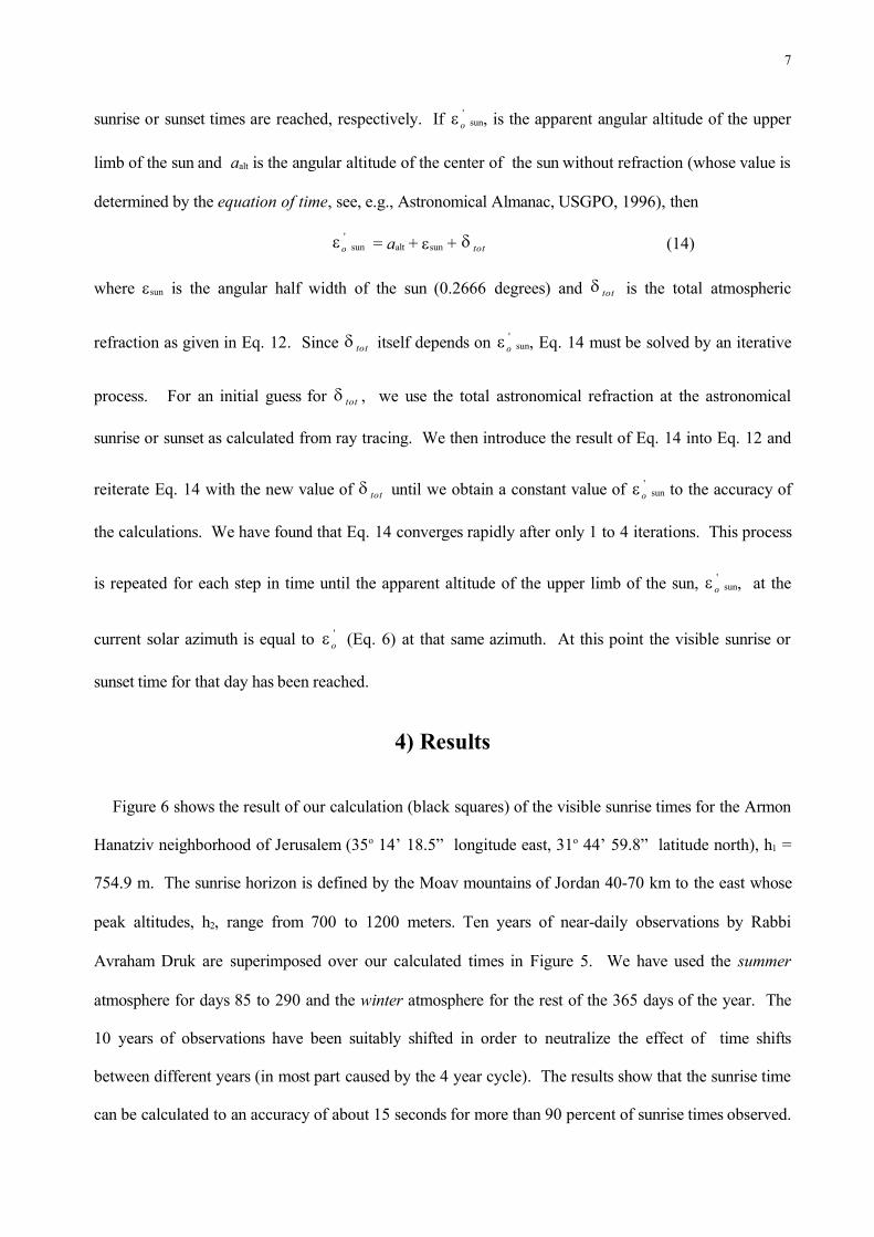
4) Results

Figure 6 shows the result of our calculation (black squares) of the visible sunrise times for the Armon

Hanatziv neighborhood of Jerusalem (35o 14’ 18.5” longitude east, 31o 44’ 59.8” latitude north), h1 =

754.9 m. The sunrise horizon is defined by the Moav mountains of Jordan 40-70 km to the east whose

peak altitudes, h2, range from 700 to 1200 meters. Ten years of near-daily observations by Rabbi

Avraham Druk are superimposed over our calculated times in Figure 5. We have used the summer

atmosphere for days 85 to 290 and the winter atmosphere for the rest of the 365 days of the year. The

10 years of observations have been suitably shifted in order to neutralize the effect of time shifts

between different years (in most part caused by the 4 year cycle). The results show that the sunrise time

can be calculated to an accuracy of about 15 seconds for more than 90 percent of sunrise times observed.

7

Comparison of observations to our calculations for other places in Israel have been consistent to the same

accuracy. It is our belief that adding a term for humidity in the index of refraction (Eq. 11) can improve

the accuracy of our calculations for the winter months. Figure 7 gives an example of the sunrise

calendars that we provide through a country-wide publication (The Bikurei Yosef Tables of the Visible

Sunrise and Sunset Times).

For a distant horizon, as that of Figure 6, elevation inaccuracies in the DTM ( 10 meters maximum,

but typically no worse than 5 meters) produce a quite negligible effect on the calculated sunrise

times. However, these inaccuracies will make the major contribution to the uncertainty in the sunrise

and sunrise times for distances less than 5 km. We therefore cannot provide tables for those cities that

have mountainous obstructions within 5 km.

The observations shown in Figure 6 are in contradiction to the conclusions of Schaefer and Liller

(1990) who claimed that it is impossible to determine the sunrise times to better than 4 min. They

obtained this conclusion by averaging observations from varying heights. However this neglects the

dependence of the rms deviation of the sunrise times on the length of the light’s air path. For example,

the length of the light’s air path to the horizon, L, for an observer of height, h1, is (Menat, 1980, his Eq.

41),

L 1h . (15)

It can be shown that a proper analysis of their data, taking account of Eq. 15, is consistent with the

observations of sunrise times for Israel.

Acknowledgments--The authors would like to acknowledge their deep gratitude to Dr. Dror Bendavid of

Midrash Bikurei Yosef for initiating and supporting this project. We would also like to thank Dr.

Mordechai Menat for providing us with his computer codes and for his useful suggestions and comments.

Finally we would like to thank Rabbi Avraham Druk for kindly providing us with his sunrise

observations. The 25 meter DTM of Israel is the copyrighted property of the Survey of Israel.

8

References

Astronomical Almanac, 1996. U.S. Government Printing Office, p. C24.

Hall, J. K., 1996. Topography and Bathymetry of the Dead Sea Depression, Tectonophysics, 266 (1-4),

pp. 177-185. This is one of thirteen papers in the Editor’s Personal Selection of the top papers

published in Tectonophysics over the past two years. It appears in full on their website at

http://www.elsevier.com/locate/tecto.

Hall, J. K., 1997a. Three-dimensional map of Israel and vicinity. Grayscale sheet of land topography at

1:500,000 scale with physiographic provinces by E. Zilberman and R. Bogoch (English Edition).

Geological Survey of Israel, Jerusalem, April 1997.

Hall, J. K., 1997b. Topography and bathymetry of the Dead Sea Depression. In: The Dead Sea - The

Lake and its Setting, eds. Tina M. Niemi, Zvi Ben-Avraham, and Joel R. Gat, Oxford Monograph on

Geology and Geophysics No. 36, Oxford University Press, New York, pp 11-21.

Hall, J. K., Schwartz, E., and Cleave, R. L. W., 1990. The Israeli DTM (Digital Terrain Map) Project.

In: Microcomputer Applications in Geology, Volume II, eds. J. Thomas Hanley and Daniel F. Merriam,

Pergamon Press, pp. 11-118. Includes FORTRAN-77 DTM program on diskette as part of the COGS

(Computer Oriented Geological Society) public-domain library.

Menat, M., 1980, Atmospheric Phenomena before and during Sunset, Applied Optics, 19, 20, pp. 3458-

3468.

9

Schaefer, B., Liller, W., 1990. Refraction near the Horizon, Publications of the Astronomical Society of

the Pacific, 102, pp.796-805.

Selby, J. E. A., et. al., Atmospheric Transmission from 0.25 to 28.5 m. Supplement LOWTRAN 3B,

In: AFGL Report TR-76-028, Air Force Systems Command, USAF, 1976.

Valley, S. L., Ed., Handbook of Geophysics and Space Environments, McGraw-Hill, New York, 1965,

Chaps. 7 and 9.

10

Figure Captions

Figure 1 Shaded relief image of the study area based upon the 25 meter DTM of Israel and eastern

Jordan (Hall 1977). Jerusalem is located in the relatively flat area in the mountains north west of the

Dead Sea. For the high places of Jerusalem, sunrise appears over the Moav Mountains in eastern Jordan,

east of the Dead Sea. (See original article for figure)

Figure 2 Depicts the path of light, in the model atmospheres, glancing off the obstruction at height, h2,

and finally reaching the observer at height h1. In the figure, the obstruction appears to make a negative

angle, 'o , with the observer’s local horizontal. Without refraction, the obstruction would make an

angle, o < 'o . Other variables are defined in the text. The dimensions are not to scale.

Figure 3 Plot of the refraction correction, corr , to the view angle, 'o , as a function of the height of

the observer, h1 for an obstruction height h2 = 500 m, and a distance to the obstruction, D = 50 km. (See

text for details.)

Figure 4 Plot of the refraction correction, corr , to the view angle, 'o , as a function of the distance,

D, to the obstruction, for an observer height h1=500 m, and an obstruction height, h2 = 500 m. (See text

for details.)

Figure 5 Plot of the total atmospheric refraction, tot , as a function of view angle, 'o , for the winter

atmosphere for 750 m h1 850 m.

11

Figure 6 Calculated sunrise times (black line) superimposed over 10 years of near daily observations of

the sunrise by Rabbi Avraham Druk from the Jerusalem neighborhood, Armon Hanatziv. (See text for

details.)

Figure 7 Example of the Bikurei Yosef Tables of the Visible Sunrise and Sunset for the city of

Jerusalem. The tables are calculated for the city of Jerusalem according to the Hebrew Calendar of the

year 5760 which spans the calendar years 1999-2000. The year 5760 is a leap year having 13 months of

length 29 or 30 days. The tables are read from top to bottom, right to left. The first time entry (the

Jewish Near Year) corresponds to September 11, 1999. As explained in the text, we are over 90%

confident that the calculated times are accurate to better than 15 seconds. Jewish religious

considerations therefore require us to add 15 seconds to each sunrise time, and subtract 15 seconds from

each sunset time. The sunrise and sunset times are then rounded to the nearest upper or lower 5 seconds,

respectively. (See original article for figure.)

12

Figure 2

13

0

0.005

0.01

0.015

0.02

0.025

0.03

-250

-100 50 200

350

500

650

800

950

1100

1250

Height of observer (m)

Ref

ract

ion

corr

ectio

n to

vie

w

angl

e (d

egre

es)

Figure 3

14

0

0.01

0.02

0.03

0.04

0.05

0.06

0.07

0 10 20 25 30 40 50 60 70 80 90 100

Distance to obstruction, D (km)

Ref

ract

ion

corr

ectio

n to

vie

w

angl

e (d

gree

s)

Figure 4

15

0

0.1

0.2

0.3

0.4

0.5

0.6

0.7

0.8

-1.00

-0.60

-0.20

0.20

0.60

1.00

1.40

1.80

2.20

2.60

3.00

3.40

3.80

4.20

4.60

5.00

View angle (degrees)

Tota

l atm

osph

eric

re

frac

tion

(deg

rees

)

Figure 5

16

2.5

3

3.5

4

4.5

5

5.5

6

6.5

1 51 101 151 201 251 301 351

days in the year 1995

minutes after th

e astron

omical sun

rise

Figure 6

17

Table Captions

Table 1 Value of coefficients in Eq. 12

Table 2 Values of coefficients in Eq. 12 for the winter atmosphere

Table 3 Values of coefficients in Eq. 12 for the summer atmosphere

18

Atmosphere i )(kmH i oiT , )(Kelvin )(, mbarP oi ta tc

1 -0.4 299.0 1013.0 -6.4231 5.29282 13.0 215.5 179.0 0.2000 -170.7413

summer 3 18.0 216.5 81.2 1.0714 -31.58034 25.0 224.0 27.7 2.2273 -15.50255 47.0 273.0 1.29 1.0000 -27.89666 50.0 276.0 0.951 -2.9000 11.24537 70.0 218.0 0.067 0.0000 0.00001 0.0 284.0 1018 -6.4000 5.39382 10.0 220.0 256.8 -0.5556 61.2602

winter 3 19.0 215.0 62.8 0.1667 -204.61234 25.0 216.0 24.3 0.2000 -169.63425 30.0 217.0 11.1 2.4500 -13.70186 50.0 266.0 0.682 -1.7500 19.00567 70.0 231.0 0.047 0.0000 0.0000

Table 1

19

h1 a(h1) b(h1) c(h1) d(h1) e(h1) f(h1)h1 1150 meters 0.16878 5104893.1 0.0148 0.0001 0.47806 0.074471050 h1 < 1150 0.16901 5105118.1 0.01575 0.00007 0.4834 0.07641950 h1 < 1050 0.16896 5105058.1 0.02169 -0.00014 0.52128 0.09025850 h1 < 950 0.16838 510445.1 0.02111 -0.00012 0.5161 0.08825750 h1 < 850 0.16876 5104876.1 0.0232 -0.00019 0.52786 0.09266650 h1 < 750 0.16907 5105295.1 0.02383 -0.00021 0.5303 0.09358550 h1 < 650 0.1691 5105256.1 0.02976 -0.00042 0.56622 0.10671450 h1 < 550 0.1696 5106268.1 0.02905 -0.00039 0.56005 0.10422350 h1 < 450 0.1691 5105319.1 0.01416 0.00011 0.46823 0.06829250 h1 < 350 0.16916 5105492.1 0.01168 0.0002 0.45241 0.06206150 h1 < 250 0.16941 5106191.1 -0.01107 0.0083 0.32072 0.005950 h1 < 150 0.16924 5105257.1 -0.00922 0.0008 0.33125 0.1087-50 h1 < 50 0.16872 5105938.1 0.0305 -0.0021 0.55065 0.10908

-150 h1 < -50 0.16872 5106064.1 0.03083 -0.00022 0.55083 0.10908h1 < -150 0.16870 5106195.1 0.03119 -0.00022 0.55118 0.10915

Table 2

20

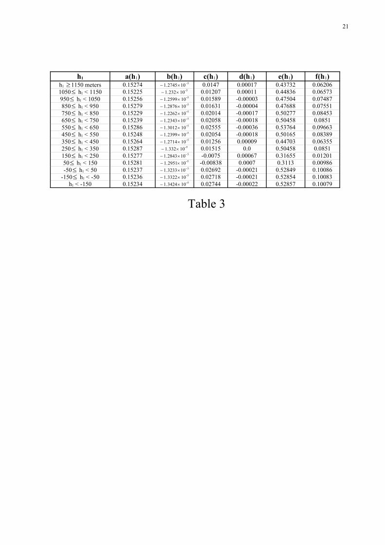
h1 a(h1) b(h1) c(h1) d(h1) e(h1) f(h1)h1 1150 meters 0.15274 5102745.1 0.0147 0.00017 0.43732 0.062061050 h1 < 1150 0.15225 510232.1 0.01207 0.00011 0.44836 0.06573950 h1 < 1050 0.15256 5102599.1 0.01589 -0.00003 0.47504 0.07487850 h1 < 950 0.15279 5102876.1 0.01631 -0.00004 0.47688 0.07551750 h1 < 850 0.15229 5102262.1 0.02014 -0.00017 0.50277 0.08453650 h1 < 750 0.15239 5102343.1 0.02058 -0.00018 0.50458 0.0851550 h1 < 650 0.15286 5103012.1 0.02555 -0.00036 0.53764 0.09663450 h1 < 550 0.15248 5102399.1 0.02054 -0.00018 0.50165 0.08389350 h1 < 450 0.15264 5102714.1 0.01256 0.00009 0.44703 0.06355250 h1 < 350 0.15287 510332.1 0.01515 0.0 0.50458 0.0851150 h1 < 250 0.15277 5102843.1 -0.0075 0.00067 0.31655 0.0120150 h1 < 150 0.15281 5102951.1 -0.00838 0.0007 0.3113 0.00986-50 h1 < 50 0.15237 5103233.1 0.02692 -0.00021 0.52849 0.10086

-150 h1 < -50 0.15236 5103322.1 0.02718 -0.00021 0.52854 0.10083h1 < -150 0.15234 5103424.1 0.02744 -0.00022 0.52857 0.10079

Table 3

21