Using applied tracer tests to predict solute transport in - Theses

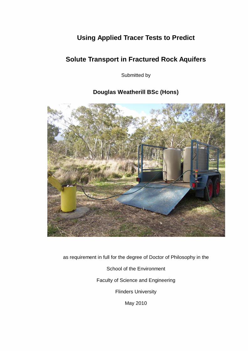
Using Applied Tracer Tests to Predict

Solute Transport in Fractured Rock Aquifers

Submitted by

Douglas Weatherill BSc (Hons)

as requirement in full for the degree of Doctor of Philosophy in the

School of the Environment

Faculty of Science and Engineering

Flinders University

May 2010

ii

Contents

Summary............................................................................................................. v

Declaration of Originality .................................................................................... vi

Acknowledgements ........................................................................................... vii

Chapter 1: Introduction ....................................................................................... 1

Objectives ........................................................................................................ 1

Synopsis of the Remaining Chapters .............................................................. 3

Chapter 2: Applied tracer tests in fractured rock: Can we predict natural

gradient solute transport more accurately than fracture and matrix

parameters? ................................................................................................. 3

Chapter 3: Discretising the fracture-matrix interface for accurate simulation

of solute transport in fractured rock.............................................................. 4

Chapter 4: Conceptual model choice for dipole tracer tests in fractured rock

..................................................................................................................... 5

Chapter 5: Interpreting dipole tracer tests in fractured rock aquifers ........... 6

Chapter 2: Applied tracer tests in fractured rock: Can we predict natural gradient

solute transport more accurately than fracture and matrix parameters? ............. 9

Abstract ........................................................................................................... 9

Introduction .................................................................................................... 10

Theory ........................................................................................................... 14

Methods......................................................................................................... 16

Forward model ........................................................................................... 16

Adding noise to the breakthrough curve .................................................... 17

Parameter estimation with PEST ............................................................... 20

iii

Breakthrough curve characteristics ............................................................ 21

Results .......................................................................................................... 22

Best-fit parameters..................................................................................... 24

Predictions ................................................................................................. 24

Uncertainty comparison: parameter estimation vs prediction ..................... 31

Discussion ..................................................................................................... 33

Conclusions ................................................................................................... 36

Notation and Units ......................................................................................... 38

References .................................................................................................... 40

Chapter 3: Discretising the fracture-matrix interface for accurate simulation of

solute transport in fractured rock ....................................................................... 42

Abstract ......................................................................................................... 42

Introduction .................................................................................................... 43

Analytical Modelling ....................................................................................... 46

Numerical Modelling ...................................................................................... 46

Results .......................................................................................................... 53

Discussion ..................................................................................................... 63

Conclusions ................................................................................................... 65


References .................................................................................................... 70

Chapter 4: Conceptual model choice for dipole tracer tests in fractured rock ... 74

Abstract ......................................................................................................... 74

Introduction .................................................................................................... 75

Methods......................................................................................................... 77

Results .......................................................................................................... 84

iv

Discussion ..................................................................................................... 89

Conclusions ................................................................................................... 92


References .................................................................................................... 96

Chapter 5: Interpreting dipole tracer tests in fractured rock aquifers ................. 99

Abstract ......................................................................................................... 99

Introduction .................................................................................................. 100

Generating Synthetic Fracture Networks ..................................................... 102

Numerical Modelling .................................................................................... 105

Analytical Modelling ..................................................................................... 109

Field Tracer Tests ....................................................................................... 118

Discussion ................................................................................................... 127

Conclusions ................................................................................................. 129

Notation and Units ....................................................................................... 132

References .................................................................................................. 134

Chapter 6: Concluding Remarks ..................................................................... 136

Summary of Findings................................................................................... 136

Further Research ........................................................................................ 138

Appendix A: Published Papers ........................................................................ 141

v

Summary

Applied tracer tests are used to measure solute transport characteristics of

fractured rock aquifers. Whilst not always mentioned in the published literature,

the ultimate purpose of the characterisation is to enable prediction of solute

transport in the aquifer. The thesis examines the potential for using forced-

gradient, applied tracer tests to predict solute transport under natural gradient

conditions in fractured rock aquifers.

Analysis of tracer tests to quantify aquifer parameters requires use of an

interpretative model. Previously it has been assumed that equivalent single

fracture and matrix parameters can be used to represent complex networks of

fractures. Given the highly heterogeneous nature of fractured rock aquifers,

tracer breakthrough curves often contain detailed features that cannot be fully

replicated by comparatively simple analytical models. This thesis examines the

parameter and prediction uncertainty that might arise from such discrepancies

between fitted breakthrough curves and complex measured data. Comparisons

are made between parameters and predictions obtained using different

analytical models and the ability of single fracture models to interpret tracer

transport in networks of fractures is examined. Methods to improve predictions

of solute transport and quantify uncertainty are identified. Also, previously

unidentified discretisation requirements are presented to enable accurate

simulation of tracer transport in numerical groundwater flow and transport

models.

vi

Declaration of Originality

I certify that this thesis does not incorporate without acknowledgement any

material previously submitted for a degree or diploma in any university; and that

to the best of my knowledge and belief it does not contain any material

previously published or written by another person except where due reference

is made in the text.

Douglas Weatherill

vii

Acknowledgements

I must say a big thank you to my supervisors, Professor Craig Simmons

(Flinders University) and Professor Peter Cook (CSIRO Land and Water) for

their scientific guidance, patience and endless support. Their constructive

criticism helped me along the road of scientific discovery and development that

is the PhD process. Both are brilliant scientists. Craig has been an inspiration

throughout my entire university education, from my undergraduate degree, to

supervising my Honours project and now supervising my PhD. He gives more

than is required and it is greatly appreciated. I look back fondly on the long days

spent in the Clare Valley with Peter as we waited for tracer to arrive!

Neville Robinson’s assistance programming and mathematical aspects of the

thesis was greatly appreciated. Neville was always willing to discuss my work

when needed.

Thank you to William Sanford (Colorado State University) for allowing me to

visit CSU and for teaching me the technical aspects required to run an applied

tracer test.

Finally, thank you to my extremely patient partner Jodie. I would not have

managed to finish this thesis without your support and encouragement.

1

Chapter 1: Introduction

Objectives

The occurrence of contaminants in groundwater systems has created a need for

means to characterise the aquifer properties affecting solute transport. Applied

tracer tests enable in-situ measurement of solute transport and a means to

estimate aquifer parameters. Tests conducted under a forced hydraulic gradient

enable more rapid measurement of tracer breakthrough than could be achieved

under ambient flow conditions and so these types of tests are usually preferred.

The interpretation of tracer tests in fractured rock aquifers presents a challenge

due to their highly heterogeneous nature. There is little in the published

literature regarding the uncertainty that is inherent in aquifer parameters

interpreted from tracer tests in fractured rock. Perhaps more importantly, the

accuracy of predictions of solute transport using made using these inferred

aquifer parameters is not understood.

The broad objectives of this thesis are to:

1) evaluate how accurately aquifer parameters can be determined from

tracer test data, given the inability of analytical models to completely

describe the complex nature of fractured rock and associated tracer

breakthrough curves;

2) quantify the impact of parameter and interpretative model uncertainty on

predictions of solute transport under lower hydraulic gradients;

2

3) identify the most effective ways to improve the accuracy of predictions of

solute transport in fractured rock aquifers made using tracer test data;

The next four chapters are presented in the form of self-contained scientific

papers. They comprise two papers which have been published in international

journals and two papers which have been prepared ready for submission to

journals. The chapters/papers are as follows:

Weatherill, D, Cook, PG, Simmons, CT and Robinson, NI, 2006. Applied tracer

tests in fractured rock: Can we predict natural gradient solute transport more

accurately than fracture and matrix parameters? Journal of Contaminant

Hydrology 88, 289-305. (Chapter 2)

Weatherill, D, Graf, T, Simmons, CT, Cook, PG, Therrien, R, and Reynolds,

DA, 2008. Discretizing the fracture-matrix interface to simulate solute transport.

Ground Water 46(4), 606-615. (Chapter 3)

Weatherill, D, McCallum, JL, Simmons, CT, Cook, PG, Robinson, NI.

Conceptual model choice for dipole tracer tests in fractured rock. In preparation.

(Chapter 4)

Weatherill, D, Simmons, CT, Cook, PG. Interpreting dipole tracer tests in

fractured rock aquifers. In preparation. (Chapter 5).

Each of the following chapters contains a review of relevant literature in the

introductory phases. Copies of the two published papers are provided in

Appendix A.

3

Synopsis of the Remaining Chapters

The following presents a synopsis of the four chapters and their main scientific

contributions.

Chapter 2: Applied tracer tests in fractured rock: Can we predict natural

gradient solute transport more accurately than fracture and matrix

parameters?

Applied tracer tests provide a means to estimate aquifer parameters in fractured

rock. The traditional approach to analysing these tests has been using a single

fracture model to find the parameter values that generate the best fit to the

measured breakthrough curve. In many cases, the ultimate aim is to predict

solute transport under the natural gradient. Usually, no confidence limits are

placed on parameter values and the impact of parameter errors on predictions

of solute transport is not discussed. The assumption inherent in this approach is

that the parameters determined under forced conditions will enable prediction of

solute transport under the natural gradient. The parameter and prediction

uncertainty that might arise from analysis of breakthrough curves obtained from

forced gradient applied tracer tests is examined. By adding noise to an exact

solution for transport in a single fracture in a porous matrix, multiple realisations

of an initial breakthrough curve are created. A least squares fitting routine is

used to obtain a fit to each realisation, yielding a range of parameter values

rather than a single set of absolute values. The suite of parameters is then used

to make predictions of solute transport under lower hydraulic gradients and the

uncertainty of estimated parameters and subsequent predictions of solute

transport is compared. Results show that predictions of breakthrough curve

4

characteristics (first inflection point time, peak arrival time and peak

concentration) for groundwater flow speeds orders of magnitude smaller than

that at which a test is conducted can sometimes be determined even more

accurately than the fracture and matrix parameters. This paradigm/philosophy

has not been explored in previous literature.

Chapter 3: Discretising the fracture-matrix interface for accurate

simulation of solute transport in fractured rock

This paper is not targeted at addressing the overall research aims of the thesis.

Rather, the paper is a by-product of work presented in chapter 5, in which

applied tracer tests are simulated in fractured rock using a numerical model.

During that process it became apparent that extremely fine spatial discretisation

was required in the matrix material immediately adjacent the simulated

fractures. This had not been previously identified in the literature. Chapter 3 is

the result of investigation into the causes and occurrences of the need for such

fine discretisation.

This paper examines the required spatial discretisation perpendicular to the

fracture-matrix interface (FMI) for numerical simulation of solute transport in

discretely-fractured porous media. The discrete fracture finite element model

HydroGeoSphere and a discrete fracture implementation of MT3DMS were

used to model solute transport in a single fracture and the results were

compared to an analytical solution. To match analytical results on the relatively

short timescales simulated in this study, very fine grid spacing perpendicular to

the FMI, of the scale of the fracture aperture, is necessary if advection and/or

5

dispersion in the fracture are high compared to diffusion in the matrix. The

requirement of such extremely fine spatial discretisation has not been

previously reported in the literature. In cases of high matrix diffusion, matching

the analytical results is achieved with larger grid spacing at the FMI. Cases

where matrix diffusion is lower can employ a larger grid multiplier moving away

from the FMI. The very fine spatial discretisation identified in this study for

cases of low matrix diffusion may limit the applicability of numerical discrete

fracture models in such cases.

Chapter 4: Conceptual model choice for dipole tracer tests in fractured

rock

Applied tracer tests provide a means to estimate fracture and matrix parameters

that determine solute transport in fractured rock. Dipole tracer tests utilise an

injection-extraction well pair to create a forced hydraulic gradient, allowing tests

to be conducted more rapidly than natural gradient tests. Tracer breakthrough is

analysed using an analytical model to find the parameters that generate the

best fit to the data. This study explores the differing interpretation that can be

drawn from a tracer test when analysed with two different models; one

assuming a dipole, the other a linear flow field. The two models are able to

produce almost identical breakthrough curves for a range of scenarios.

Comparison of the parameters required to create matching breakthrough curves

demonstrates the non-uniqueness of the 1-D and dipole interpretations,

resulting in large parameter uncertainty. Considering that neither of the

conceptual models incorporates the complexity of a real fracture network, it is

expected that analytically interpreted parameters may be as different, or more

6

different from reality as they are from those interpreted with a different analytical

model. Given the complex nature of fractured rock systems and the many

unknown fracture and matrix properties involved therein, this study highlights

the benefit of incorporating multiple conceptual models in the analyses of dipole

tracer tests conducted in fractured rock.

Chapter 5: Interpreting dipole tracer tests in fractured rock aquifers

Dipole tracer tests, where transport of applied tracer is measured in a steady

state flow field between an injection-extraction well pair, provide a means to

measure solute transport through in-situ aquifer material. A dipole flow field

allows sampling of a large volume of aquifer and the forced gradient enables

rapid measurement of tracer transport. The measured tracer breakthrough

curve is used to infer aquifer properties, usually using an analytical model. For

tests conducted in fractured rock aquifers it is usually assumed that equivalent

single fracture and matrix parameters can be used to represent the whole

network. The extent to which the complex geometry of a fracture network

affects the interpretation of a dipole tracer test is not known.

The previous chapter examined the different interpretations that can arise when

using two single fracture analytical models. This study builds on those results to

look at the performance of the models when used to interpret tracer tests

conducted in networks of fractures. The first part of this study examines the

performance of two single fracture analytical models when used to interpret

simulated dipole tracer tests conducted in hypothetical three-dimensional

fracture networks. Initially a single dipole tracer test is simulated numerically in

7

a hypothetical fracture network. The analytical models are calibrated to the

modelled tracer breakthrough curve and used to predict solute transport under a

much lower hydraulic gradient. The predicted solute transport is then compared

to the ‘real’ simulated transport. In this way the consequences of the single

fracture approximation and associated flow geometry of the two interpretative

analytical models are identified. Both the analytical models are able to produce

good fits to the initial tracer test data, but the predictive performance of the

models decreases as they are used to predict transport under increasingly

lower hydraulic gradients. The study then examines how the predictive

capability of the analytical models is improved if additional information is

available to calibrate them. The value of the following is examined: (a) an extra

tracer test at either higher or lower hydraulic gradient, (b) an additional tracer

with a different diffusion coefficient included in the initial tracer test and (c)

knowledge of the length of the shortest fracture flow path between the injection

and extraction wells (rather than an assumption of a straight line). Results

indicated that predictions could be most improved by conducting an additional

test at a lower injection and extraction rate.

The second section of this study applies the methodology used in the

hypothetical fracture networks to real dipole tracer tests conducted in the Clare

Valley, South Australia. Application of the methodology to the field environment

introduces additional variations between the assumptions of the analytical

models and the reality of the field setting. In correlation with the results for the

synthetic fracture networks, the predictive performance of the calibrated single

fracture models was found to decrease as the hydraulic gradient of predictive

8

scenarios was decreased. However, hydraulic data indicated that the

application of dipoles at different pumping rates resulted in significantly different

dewatering of the aquifer near the extraction well and therefore tests at different

hydraulic gradients were not sampling the same fracture pathways between the

well pair. This phenomenon, combined with the findings from the hypothetical

fracture networks suggests that dipole tracer tests in unconfined aquifers should

be performed at the lowest feasible pumping rates where the aim is to predict

solute transport under ambient groundwater flow conditions.

9

Chapter 2: Applied tracer tests in fractured rock: Can

we predict natural gradient solute transport more

accurately than fracture and matrix parameters?

The work presented in this chapter can be found in the following:

Weatherill, D, Cook, PG, Simmons, CT and Robinson, NI, 2006. Applied tracer

tests in fractured rock: Can we predict natural gradient solute transport more

accurately than fracture and matrix parameters? Journal of Contaminant

Hydrology 88, 289-305.

Abstract


rock. The traditional approach to analysing these tests has been using a single

fracture model to find the parameter values that generate the best fit to the

measured breakthrough curve. In many cases, the ultimate aim is to predict

solute transport under the natural gradient. Usually, no confidence limits are

placed on parameter values and the impact of parameter errors on predictions

of solute transport is not discussed. The assumption inherent in this approach is

that the parameters determined under forced conditions will enable prediction of

solute transport under the natural gradient. This paper considers the parameter

and prediction uncertainty that might arise from analysis of breakthrough curves

obtained from forced gradient applied tracer tests. By adding noise to an exact

solution for transport in a single fracture in a porous matrix we create multiple

realisations of an initial breakthrough curve. A least squares fitting routine is

10

used to obtain a fit to each realisation, yielding a range of parameter values

rather than a single set of absolute values. The suite of parameters is then used

to make predictions of solute transport under lower hydraulic gradients and the

uncertainty of estimated parameters and subsequent predictions of solute

transport is compared. The results of this study show that predictions of

breakthrough curve characteristics (first inflection point time, peak arrival time

and peak concentration) for groundwater flow speeds orders of magnitude

smaller than that at which a test is conducted can sometimes be determined

even more accurately than the fracture and matrix parameters.

Introduction


rock. Tests conducted under a forced hydraulic gradient, for example

Novakowski et al. (1985) and Sanford et al. (2002), enable more rapid

measurement of tracer breakthrough than could be achieved under ambient

flow conditions and so these types of tests are usually preferred.

Many fractured rock tracer tests are analysed with a single fracture model,

regardless of whether they were conducted in a single fracture or through a

network of fractures. The model may be optimised to fit the breakthrough curve

but the parameters, and indeed the model itself, may not be a good

representation of reality. An extreme case is when multiple peaks are observed

such as those reported by Abelin et al. (1991) and Jakob and Hadermann

(1994). A single flow path model can never describe such a system correctly,

although a best-fit model could be obtained. Similarly, the choice of whether to

11

model variable apertures, ambient flow and other processes will impact upon

the integrity of the interpretation.

Complex models incorporating many processes and therefore many parameters

have greater potential to generate non-unique solutions, whereas simpler

models may not be able to adequately match the data. Thus due to the complex

nature of fractured rock, analysis of tracer tests conducted in fracture networks

is subject to the potential for large errors in the analysis phase, as well as the

measurement errors associated with any experimental procedure. Maloszewski

and Zuber (1983) go as far as saying “The great number of non-disposable

parameters make a correct interpretation of tracer experiments impossible.”

Knowing that our models are always a simplification of reality, it is probably

optimistic to place exact values on the parameters obtained from them. There

may be many parameter sets that will generate an approximation to a

breakthrough curve, but a conventional best-fit inversion approach yields a

single set of parameters. For example, for a dipole tracer test in an isolated

fracture Novakowski et al. (1985) present parameter values of effective fracture

aperture and dispersivity based on a single fracture model with no matrix

diffusion. The authors state that due to the goodness of the fit over the entire

data range and the sensitivity of the model to dispersivity that their fit is unique,

but they do not quantify the errors on the parameters. Similarly, for a dipole

tracer test in a fracture network Sanford et al. (2002) present best-fit parameter

values for fracture path length, fracture aperture, maximum water velocity and

dispersivity for a single fracture model with dispersion and matrix diffusion.

Whilst these authors show that different parameter values do not match the

12

measured breakthrough curves quite as well as the best fit parameters do, they

do not quantify the errors on the parameter values. Numerous examples of

analyses of tracer tests can be found in the literature in which the absolute

parameter values that optimise the fit between a modelled breakthrough curve

and the measured one are found. Whilst some authors make comparisons

between these parameter values and those obtained using other means or at

other sites, errors are rarely quantified. With many assumptions made in

analysing tracer test data, it is valuable to obtain a range of parameter sets that

fit the data within a prescribed tolerance level and to ascertain the uncertainty

on these estimations. This is likely to be more useful than a set of absolute

parameter values where error or uncertainty is not known at all.

There is an additional factor that warrants attention. Typically, forced gradient

tracer tests are conducted to enable prediction of solute transport under the

natural gradient (such as leakage from a waste disposal site). The fracture and

matrix parameters obtained from the inversion process are usually a step

towards prediction at lower velocities. Yet we have been unable to find any

previous studies which have considered the effect that the errors on these

parameters may have for prediction. If prediction is the ultimate aim then the

errors on the predictions are important.

This paper considers the uncertainty on parameters and predictions that might

arise from analysis of breakthrough curves obtained from forced gradient

applied tracer tests. In order to simulate the complexity observed in field data,

we add noise to an exact solution to create multiple realisations of an initial

13

breakthrough curve simulated using the analytical solution of Tang et al. (1981).

The best fit for each realisation is found using a least squares fitting routine,

yielding a range of parameter values rather than a single set of absolute values.

The suite of parameters is then used to make a range of predictions of solute

transport under lower hydraulic gradients. The uncertainty of estimated

parameters from tracer test breakthrough curves and subsequent predictions of

solute transport at lower groundwater velocities are compared.

Although this study interprets data generated with a particular single fracture

model, the same process is applicable to other models. The purpose of this

study is not to provide an absolute description of the behaviour of solute

transport in fractured rock, but rather to demonstrate that the uncertainty

associated with solute transport predictions under natural gradients may, in

some cases, be smaller than the uncertainty of parameters estimated from

breakthrough curves. This paradigm/philosophy has not been explored in

previous literature.

The objectives of this study are to identify:

1) How accurately individual parameters can be determined from a

breakthrough curve;

2) How accurately can predictions be made of solute transport under lower

hydraulic gradients using parameters obtained from fitting a forced gradient

breakthrough curve;

3) How the uncertainties on parameters compare to those on predicted solute

transport.

14

Theory

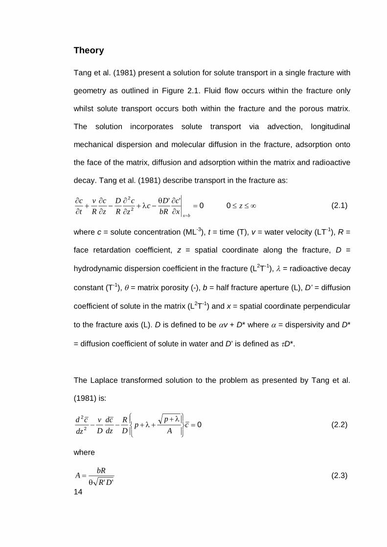
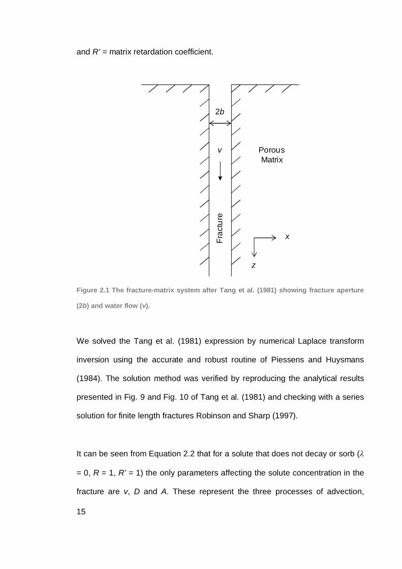
Tang et al. (1981) present a solution for solute transport in a single fracture with

geometry as outlined in Figure 2.1. Fluid flow occurs within the fracture only

whilst solute transport occurs both within the fracture and the porous matrix.

The solution incorporates solute transport via advection, longitudinal

mechanical dispersion and molecular diffusion in the fracture, adsorption onto

the face of the matrix, diffusion and adsorption within the matrix and radioactive

decay. Tang et al. (1981) describe transport in the fracture as:

zxc

bRDc

zc

RD

zc

Rv

tc

bx

002

2 '' (2.1)

where c = solute concentration (ML-3), t = time (T), v = water velocity (LT-1), R =

face retardation coefficient, z = spatial coordinate along the fracture, D =

hydrodynamic dispersion coefficient in the fracture (L2T-1), = radioactive decay

constant (T-1), = matrix porosity (-), b = half fracture aperture (L), D’ = diffusion

coefficient of solute in the matrix (L2T-1) and x = spatial coordinate perpendicular

to the fracture axis (L). D is defined to be v + D* where = dispersivity and D*

= diffusion coefficient of solute in water and D’ is defined as D*.

The Laplace transformed solution to the problem as presented by Tang et al.

(1981) is:

02

2

cA

pp

DR

dzcd

Dv

dzcd (2.2)

where

''DRbRA (2.3)

15

and R’ = matrix retardation coefficient.

v

2b

z

xFrac

ture

Porous Matrix

Figure 2.1 The fracture-matrix system after Tang et al. (1981) showing fracture aperture

(2b) and water flow (v).

We solved the Tang et al. (1981) expression by numerical Laplace transform

inversion using the accurate and robust routine of Piessens and Huysmans

(1984). The solution method was verified by reproducing the analytical results

presented in Fig. 9 and Fig. 10 of Tang et al. (1981) and checking with a series

solution for finite length fractures Robinson and Sharp (1997).

It can be seen from Equation 2.2 that for a solute that does not decay or sorb (

= 0, R = 1, R’ = 1) the only parameters affecting the solute concentration in the

fracture are v, D and A. These represent the three processes of advection,

16

dispersion and matrix diffusion respectively. By assuming that hydrodynamic

dispersion within the fracture is dominated by the mechanical dispersion

component (ie v >> D*) the 6 parameters (v, , D*, , and b) can be reduced

to v, and A, where A is now simplified to A = b/ D’1/2.

Methods

Forward model

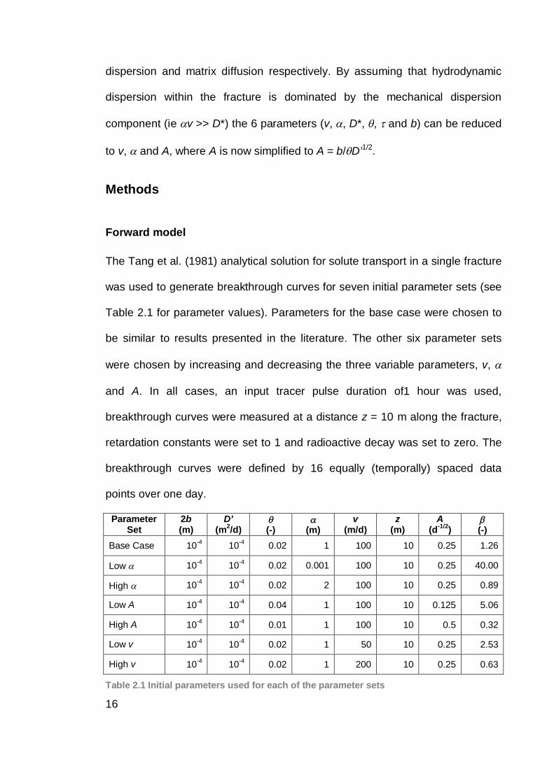
The Tang et al. (1981) analytical solution for solute transport in a single fracture

was used to generate breakthrough curves for seven initial parameter sets (see

Table 2.1 for parameter values). Parameters for the base case were chosen to

be similar to results presented in the literature. The other six parameter sets

were chosen by increasing and decreasing the three variable parameters, v,

and A. In all cases, an input tracer pulse duration of1 hour was used,

breakthrough curves were measured at a distance z = 10 m along the fracture,

retardation constants were set to 1 and radioactive decay was set to zero. The

breakthrough curves were defined by 16 equally (temporally) spaced data

points over one day.

Parameter Set

2b (m)

D’ (m2/d)

(-)

(m)

v (m/d)

z (m)

A (d-1/2)

(-)

Base Case 10-4 10-4 0.02 1 100 10 0.25 1.26

Low 10-4 10-4 0.02 0.001 100 10 0.25 40.00

High 10-4 10-4 0.02 2 100 10 0.25 0.89

Low A 10-4 10-4 0.04 1 100 10 0.125 5.06

High A 10-4 10-4 0.01 1 100 10 0.5 0.32

Low v 10-4 10-4 0.02 1 50 10 0.25 2.53

High v 10-4 10-4 0.02 1 200 10 0.25 0.63

Table 2.1 Initial parameters used for each of the parameter sets

17

Adding noise to the breakthrough curve

In order to determine the sensitivity of the breakthrough curves to different

hydrogeologic parameters, 100 realisations were generated from each

parameter set, each with different added random noise of a specified level

(ranging from 5% to 20%) added to each data point. The effect of the applied

noise level is examined in this study. By progressively increasing the number of

realisations employed, it was found that 100 realisations were more than

sufficient to achieve converged average fitted parameters.

We first attempted to understand how such noise might appear in field tracer

experiments. Clearly, the interpreted differences between a real breakthrough

curve and any mathematical fit (herein after called “noise”) are a function of

numerous factors including (1) measurement error in instruments, field data

collection and subsequent analyses, (2) the choice of conceptual and hence

mathematical model used to fit the field data, (3) the inherent complexity (at

many spatial and temporal scales) in heterogeneous geologic field settings that

is not captured by the mathematical model employed, and (4) the fitting

algorithms and convergence criteria used to define when an optimised fit to the

data has been obtained. An analysis of typical tracer test results presented by

Sanford et al. (2002) reveals an average residual of 19% (with residual mode =

2 to 4%) for bromide and 18% (with residual mode = 6 to 8%) for helium, where

the residual is defined as the absolute value of (cmeasured – cmodelled)/cmeasured. In

comparing these average and modes, it is clear that the average is somewhat

larger owing to a small number of data points which have large associated

residuals. This comparison with field data is fairly crude and is based upon one

18

case only. However, it suggests that the level of noise applied in this study is

indeed likely in a field based scenario. It was difficult to determine what

distribution these residuals followed due to the limited number of points in the

breakthrough curves. This problem is expected to arise in the analysis of most,

if not all, previously published breakthrough curves due to the typically limited

number of measurement points and a resultant inability to construct the precise

statistical distribution of residuals. To the authors best knowledge the nature of

such residuals (i.e., discrepancies between measured and modelled data) are

rarely, if ever, known and have not been the subject of previous investigation.

Therefore, the choice of noise type used in this study (white noise) might be

arbitrary, but the aim of this study is intended to be demonstrative rather than

absolutely quantitative. Therefore, the key trends and outcomes of the study are

expected to be qualitatively similar regardless of the choice of noise distribution

employed.

Random numbers were obtained using a random number generator in which

each random number had an equal probability of falling anywhere between 0

and 1 (white noise). The level of noise was specified such that the maximum

deviation from the initial data was a chosen percentage of the initial data value

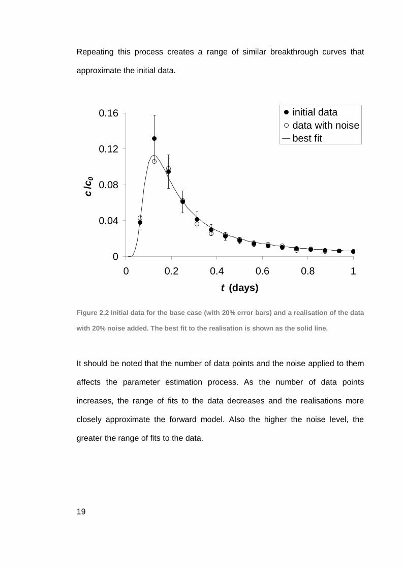
itself. This process is illustrated in Figure 2.2, where the initial data for the base

case is shown as well as a realisation of the data with 20% noise added. The

best-fit breakthrough curve for the realisation does not pass directly through the

initial data points, but is similar to the initial curve. Adding noise creates a fit that

is not the absolute best fit to the initial data, but that still approximates it.

19

Repeating this process creates a range of similar breakthrough curves that

approximate the initial data.

0

0.04

0.08

0.12

0.16

0 0.2 0.4 0.6 0.8 1t (days)

c/c

0

initial datadata with noisebest fit

Figure 2.2 Initial data for the base case (with 20% error bars) and a realisation of the data

with 20% noise added. The best fit to the realisation is shown as the solid line.

It should be noted that the number of data points and the noise applied to them

affects the parameter estimation process. As the number of data points

increases, the range of fits to the data decreases and the realisations more

closely approximate the forward model. Also the higher the noise level, the

greater the range of fits to the data.

20

Parameter estimation with PEST

PEST (Doherty, 2004) is a model-independent parameter estimation program.

PEST finds the parameters that minimise the squared sum of weighted

residuals between the target and fitted data values. In our study, equal

weighting was assigned to all data values. PEST has a number of ways of

determining when it has found optimal parameter values (or done the best it

can). The ideal termination criterion is that the objective function (squared sum

of weighted residuals) reaches zero. This means that the parameters have been

found such that the modelled values exactly match the measured values. This

cannot always be achieved, so other termination criteria are required. In our

study, if 4 iterations pass since the lowest objective function value, or if the

lowest 4 objective function values are within 0.005, relative to the minimum

objective function, of each other, PEST stops. Otherwise if 4 iterations pass in

which the largest relative parameter value change has been less than or equal

to 0.01, PEST terminates execution. As a final criterion for ending execution,

PEST will stop after 30 iterations. For further detail on PEST, the reader is

referred to Doherty (2004).

During the fitting process, bounds must be placed on the parameters. In order

to find a representative range of possible fits to the data, large bounds were

placed on the parameters so that they would not interfere with the parameter

estimation process, except in cases where parameters must be logically

bounded (ie , v, A 0).

21

Breakthrough curve characteristics

In order to quantify the differences between breakthrough curves, properties

that would describe the shape and behaviour of a breakthrough curve were

required. Three characteristics were used; time to the first inflection point (ti1),

time to the peak concentration (tp) and the peak concentration (cp). These three

characteristics are the most basic descriptors of a breakthrough curve and can

most easily be obtained from tracer test data. Other indicators such as mass

recovery may be more difficult to quantify accurately and harder to interpret due

to mass losses that result from non-recovered tracer, long breakthrough curve

tails resulting from the flow geometry induced by the forced gradient and/or

matrix diffusion. Thus, mass recovery, whilst theoretically determinable was not

used here due to the complications associated with quantifying it under field

conditions.

In order to quantify the spread of parameter values and subsequent predictions

of the breakthrough characteristics, the coefficients of variation (CV = standard

deviation / mean) of parameter values and predicted characteristics were found

for each set of realisations. This enables uniform and consistent comparison of

the confidence in different estimated parameters/predictions regardless of their

numerical values.

In order to determine the accuracy of predictions based on parameters obtained

under a forced gradient (high water velocity), breakthrough curves were

generated using parameters from each of the best-fit realisations at several

slower groundwater flow velocities. It is assumed here that the hydraulic

22

pressures associated with the different hydraulic gradients have no effect on the

fracture apertures or other physical properties of the system other than to

change the flow velocity of water in the fracture. Characteristics ti1, tp and cp

were determined at vpr = 1, 0.3, 0.1, 0.03, 0.01, 0.003, 0.001, 0.0003 and

0.0001 where:

)( fittedtest

predictionpr v

vv (2.4)

where vprediction = prediction water velocity (LT-1) and vtest (fitted) = fitted water

velocity under the forced gradient (LT-1).

Scaling down to vpr = 0.0001 is sufficient to cover the scaling required for most

current forced gradient tracer tests. Love et al. (2002) quote hydraulic gradients

ranging from 0.005 to 0.1 for a fractured rock catchment. Consider a tracer test

conducted between two wells 10 m apart in such a system. In order to require a

scaling factor of vpr = 0.0001, a head difference of 500 m to 10 000 m between

the two wells would need to be imposed. This head difference is unrealistically

large and therefore suggests that the range of vpr employed in this study more

than adequately covers the range likely to be encountered in realistic field

settings.

Results

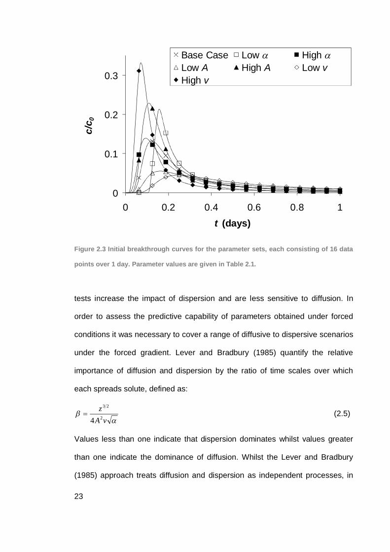
Figure 2.3 shows the breakthrough curves for the seven initial parameter sets

outlined in Table 2.1. In fractured rock systems, particularly where the porosity

of the matrix is greater than the fracture porosity, solute transport over long time

scales is dominated by matrix diffusion. By applying a forced gradient, tracer

23

0

0.1

0.2

0.3

0 0.2 0.4 0.6 0.8 1t (days)

c/c 0

Base Case Low High Low A High A Low vHigh v

Figure 2.3 Initial breakthrough curves for the parameter sets, each consisting of 16 data

points over 1 day. Parameter values are given in Table 2.1.

tests increase the impact of dispersion and are less sensitive to diffusion. In

order to assess the predictive capability of parameters obtained under forced

conditions it was necessary to cover a range of diffusive to dispersive scenarios

under the forced gradient. Lever and Bradbury (1985) quantify the relative

importance of diffusion and dispersion by the ratio of time scales over which

each spreads solute, defined as:

vAz2

23

4 (2.5)

Values less than one indicate that dispersion dominates whilst values greater

than one indicate the dominance of diffusion. Whilst the Lever and Bradbury

(1985) approach treats diffusion and dispersion as independent processes, in

24

contrast to the coupled solution of Tang et al. (1981), it gives an indication of

the relative dominance of the processes. The parameters chosen for this study

cover a range of diffusive versus dispersive scenarios, with ranging from

0.316 to 40, with the base case close to unity at 1.26. A complete set of values

for is presented in Table 2.1.

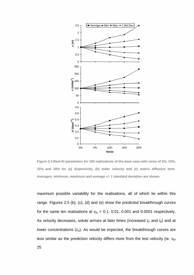
Best-fit parameters

Figure 2.4 shows the range in optimised parameter values obtained for the base

case with noise levels of 5%, 10%, 15% and 20%. As would be expected,

increased noise broadens the range of possible parameter values for , v and

A. For the case of dispersivity, it can be seen that at a 20% noise level one

standard deviation (0.472 m) is almost half as large as the average parameter

value (1.07 m) itself. The average values for , v and A remain close to the

initial values despite the range of values increasing. However, if sufficient noise

was applied, the parameter bounds may be reached (ie , v, A 0) causing

parameter biasing.

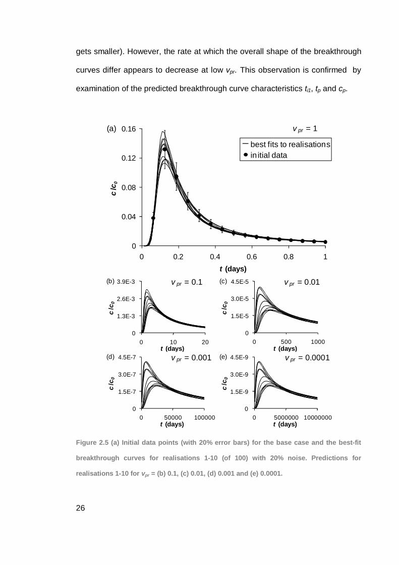
Predictions

Predictions of solute transport under slower groundwater velocities were made

using the same solute source duration and the best-fit parameters for each

realisation (with water velocity scaled by vpr). Figure 2.5 (a) shows the initial

data points for the base case and best-fit breakthrough curves for the first ten

realisations with a noise level of 20%. All breakthrough curves could be

considered to fit the initial data. The noise bounds are shown to indicate the

25

0

0.5

1

1.5

2

2.5

(m)

Average Min Max 1 Std Dev

0

50

100

150

200

250

v(m

day-1

)

0

0.1

0.2

0.3

0.4

0.5

0.6

0% 5% 10% 15% 20%Noise

A(d

ays-1

/2)

Figure 2.4 Best-fit parameters for 100 realisations of the base case with noise of 5%, 10%,

15% and 20% for (a) dispersivity, (b) water velocity and (c) matrix diffusion term.

Averages, minimum, maximum and average +/- 1 standard deviation are shown.

maximum possible variability for the realisations, all of which lie within this

range. Figures 2.5 (b), (c), (d) and (e) show the predicted breakthrough curves

for the same ten realisations at vpr = 0.1, 0.01, 0.001 and 0.0001 respectively.

As velocity decreases, solute arrives at later times (increased ti1 and tp) and at

lower concentrations (cp). As would be expected, the breakthrough curves are

less similar as the prediction velocity differs more from the test velocity (ie. vpr

26

gets smaller). However, the rate at which the overall shape of the breakthrough

curves differ appears to decrease at low vpr. This observation is confirmed by

examination of the predicted breakthrough curve characteristics ti1, tp and cp.

0

0.04

0.08

0.12

0.16

0 0.2 0.4 0.6 0.8 1t (days)

c/c

0

best fits to realisationsinitial data

v pr = 1(a)

0

1.3E-3

2.6E-3

3.9E-3

0 10 20t (days)

c/c

0

v pr = 0.1(b)

0

1.5E-5

3.0E-5

4.5E-5

0 500 1000t (days)

c/c

0

v pr = 0.01(c)

0

1.5E-7

3.0E-7

4.5E-7

0 50000 100000t (days)

c/c

0

v pr = 0.001(d)

0

1.5E-9

3.0E-9

4.5E-9

0 5000000 10000000t (days)

c/c

0

v pr = 0.0001(e)

Figure 2.5 (a) Initial data points (with 20% error bars) for the base case and the best-fit

breakthrough curves for realisations 1-10 (of 100) with 20% noise. Predictions for

realisations 1-10 for vpr = (b) 0.1, (c) 0.01, (d) 0.001 and (e) 0.0001.

27

0%

20%

40%

60%

80%

100%

CV

( t i1)

5% 10% 15% 20%

0%

20%

40%

60%

80%

100%C

V( t p

)

0%

20%

40%

60%

80%

100%

0.0001 0.001 0.01 0.1 1v pr

CV

(cp

)

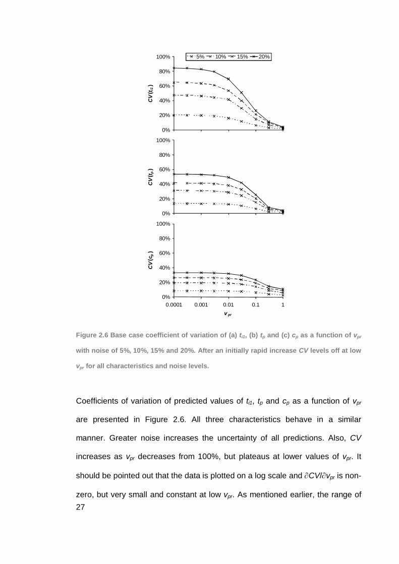
Figure 2.6 Base case coefficient of variation of (a) ti1, (b) tp and (c) cp as a function of vpr

with noise of 5%, 10%, 15% and 20%. After an initially rapid increase CV levels off at low

vpr for all characteristics and noise levels.

Coefficients of variation of predicted values of ti1, tp and cp as a function of vpr

are presented in Figure 2.6. All three characteristics behave in a similar

manner. Greater noise increases the uncertainty of all predictions. Also, CV

increases as vpr decreases from 100%, but plateaus at lower values of vpr. It

should be pointed out that the data is plotted on a log scale and CV/ vpr is non-

zero, but very small and constant at low vpr. As mentioned earlier, the range of

28

vpr values covered in this study is greater than that which would be used in

current practice. The plots cannot be extrapolated back to vpr = 0 as this is

meaningless. The plateauing is explained by the lessening impact of dispersivity

on the solution at lower velocity. The behaviour asymptotes towards one in

which only v and A have an impact. For example, in the 20% noise case, the

CV values are 44% for , 32% for v and 36% for A. With the dispersion

coefficient dominated by v, as velocity decreases, so does the dispersion

coefficient. In addition, slower water flow allows greater matrix diffusion,

increasing the dominance of A on the solution. Overall at lower water velocity

(and lower vpr) the solution is governed more by the better constrained

parameters (A and v) and less by the poorest defined ( ).

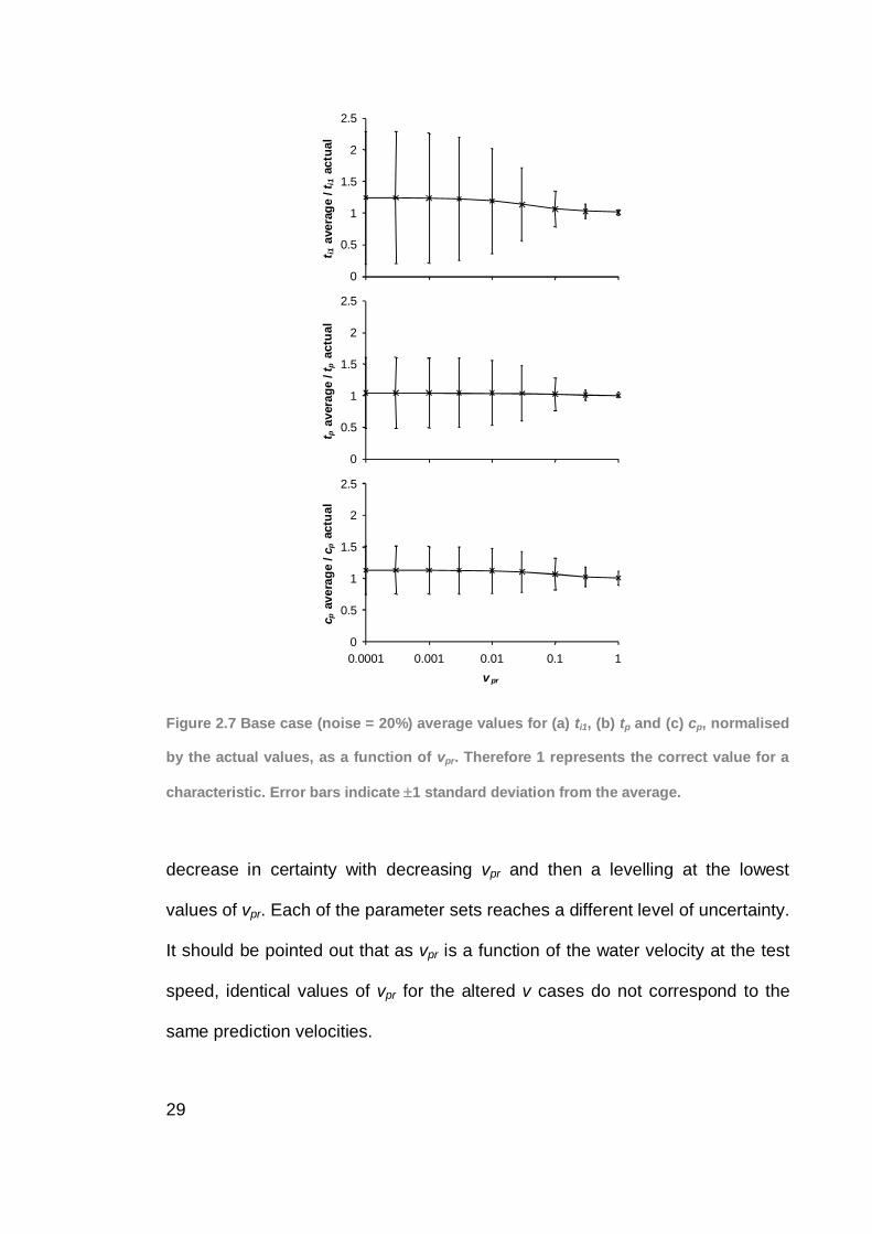
In order to demonstrate the range of predicted values around the actual values,

Figure 2.7 shows the average predicted characteristic values normalised by the

actual values with error bounds of +/- one standard deviation. The range of

predictions is best constrained at the test speed and broadens with decreasing

vpr. Minor biasing of average predictions is evident. Both averages and ranges

of predictions plateau for lower vpr.

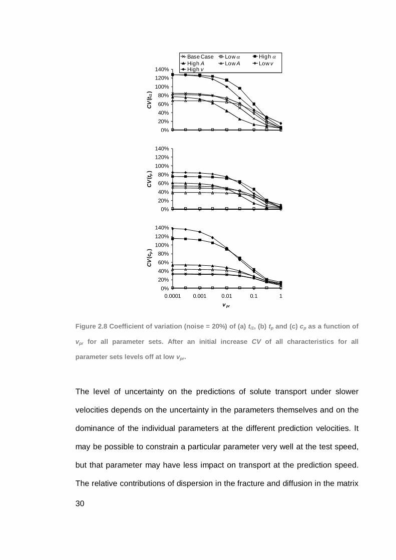
To test whether the results obtained for the base case apply more generally, a

further 6 parameter sets were tested using the same procedure used for the

base case, but with decreased and increased , A and v (Table 2.1). Figure 2.8

shows the behaviour of the predicted transport characteristics. As with the base

case, breakthrough curve characteristics for all parameter sets display a

29

0

0.5

1

1.5

2

2.5

t i1av

erag

e / t

i1ac

tual

0

0.5

1

1.5

2

2.5

t pav

erag

e / t

pac

tual

0

0.5

1

1.5

2

2.5

0.0001 0.001 0.01 0.1 1v pr

c pav

erag

e / c

pac

tual

Figure 2.7 Base case (noise = 20%) average values for (a) ti1, (b) tp and (c) cp, normalised

by the actual values, as a function of vpr. Therefore 1 represents the correct value for a

characteristic. Error bars indicate 1 standard deviation from the average.

decrease in certainty with decreasing vpr and then a levelling at the lowest

values of vpr. Each of the parameter sets reaches a different level of uncertainty.

It should be pointed out that as vpr is a function of the water velocity at the test

speed, identical values of vpr for the altered v cases do not correspond to the

same prediction velocities.

30

0%20%40%60%80%

100%120%140%

CV

( t i1)

Base Case Low High Low AHigh A Low v

High v

0%20%40%60%80%

100%120%140%

CV

( t p)

0%20%40%60%80%

100%120%140%

0.0001 0.001 0.01 0.1 1v pr

CV

(cp)

Figure 2.8 Coefficient of variation (noise = 20%) of (a) ti1, (b) tp and (c) cp as a function of

vpr for all parameter sets. After an initial increase CV of all characteristics for all

parameter sets levels off at low vpr.

The level of uncertainty on the predictions of solute transport under slower

velocities depends on the uncertainty in the parameters themselves and on the

dominance of the individual parameters at the different prediction velocities. It

may be possible to constrain a particular parameter very well at the test speed,

but that parameter may have less impact on transport at the prediction speed.

The relative contributions of dispersion in the fracture and diffusion in the matrix

31

at the test and prediction velocities and the degree to which they can be

identified determines the accuracy of the predictions.

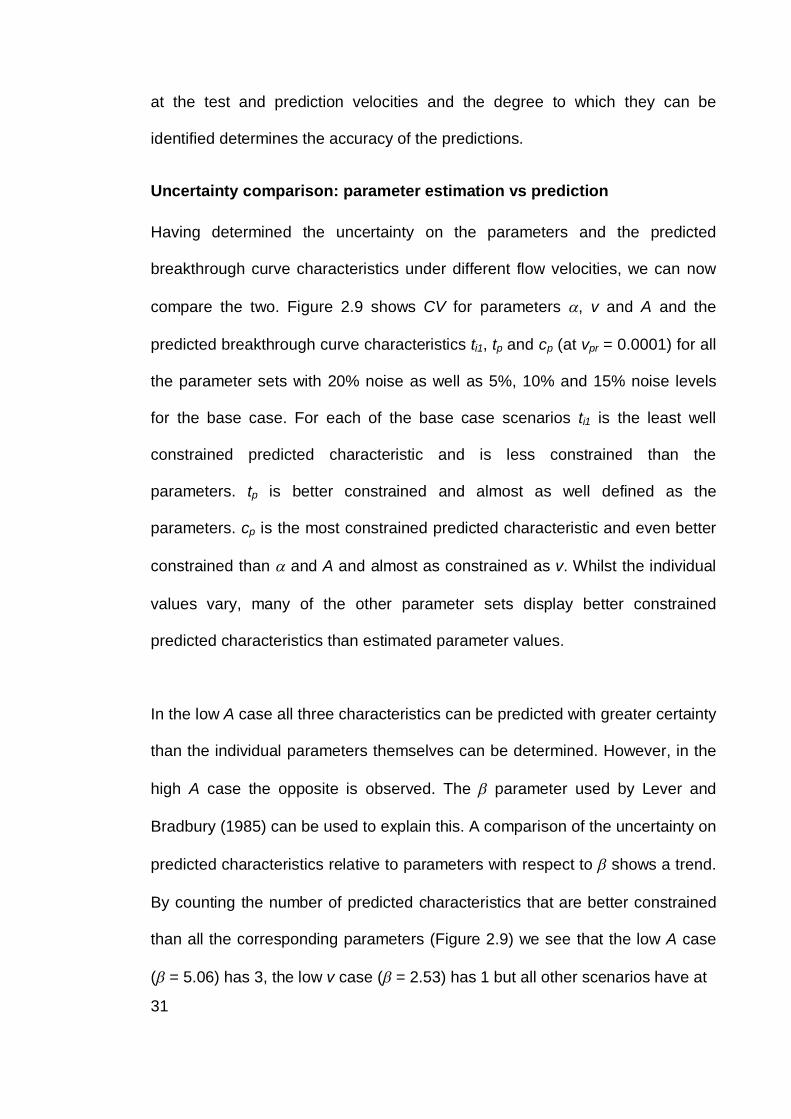
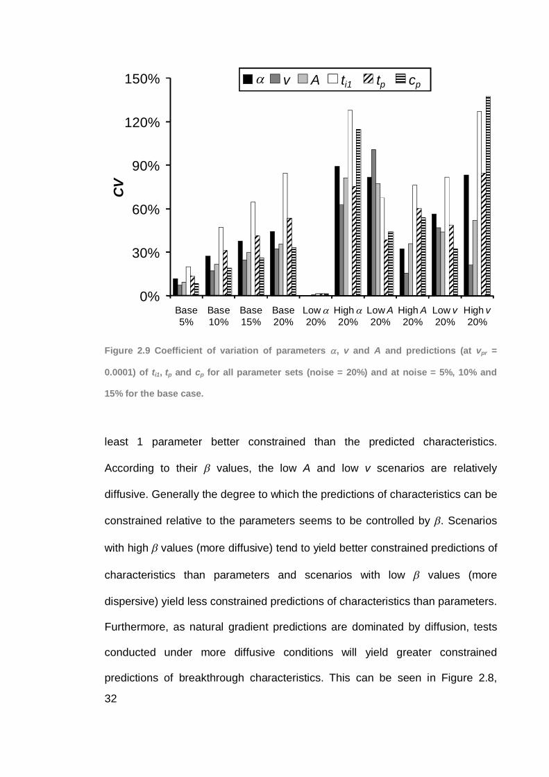
Uncertainty comparison: parameter estimation vs prediction

Having determined the uncertainty on the parameters and the predicted

breakthrough curve characteristics under different flow velocities, we can now

compare the two. Figure 2.9 shows CV for parameters , v and A and the

predicted breakthrough curve characteristics ti1, tp and cp (at vpr = 0.0001) for all

the parameter sets with 20% noise as well as 5%, 10% and 15% noise levels

for the base case. For each of the base case scenarios ti1 is the least well

constrained predicted characteristic and is less constrained than the

parameters. tp is better constrained and almost as well defined as the

parameters. cp is the most constrained predicted characteristic and even better

constrained than and A and almost as constrained as v. Whilst the individual

values vary, many of the other parameter sets display better constrained

predicted characteristics than estimated parameter values.

In the low A case all three characteristics can be predicted with greater certainty

than the individual parameters themselves can be determined. However, in the

high A case the opposite is observed. The parameter used by Lever and

Bradbury (1985) can be used to explain this. A comparison of the uncertainty on

predicted characteristics relative to parameters with respect to shows a trend.

By counting the number of predicted characteristics that are better constrained

than all the corresponding parameters (Figure 2.9) we see that the low A case

( = 5.06) has 3, the low v case ( = 2.53) has 1 but all other scenarios have at

32

0%

30%

60%

90%

120%

150%

Base5%

Base10%

Base15%

Base20%

Low 20%

High 20%

Low A20%

High A20%

Low v20%

High v20%

CV

v A ti1 tp cp

Figure 2.9 Coefficient of variation of parameters , v and A and predictions (at vpr =

0.0001) of ti1, tp and cp for all parameter sets (noise = 20%) and at noise = 5%, 10% and

15% for the base case.

least 1 parameter better constrained than the predicted characteristics.

According to their values, the low A and low v scenarios are relatively

diffusive. Generally the degree to which the predictions of characteristics can be

constrained relative to the parameters seems to be controlled by . Scenarios

with high values (more diffusive) tend to yield better constrained predictions of

characteristics than parameters and scenarios with low values (more

dispersive) yield less constrained predictions of characteristics than parameters.

Furthermore, as natural gradient predictions are dominated by diffusion, tests

conducted under more diffusive conditions will yield greater constrained

predictions of breakthrough characteristics. This can be seen in Figure 2.8,

33

where the least constrained predictions of characteristics occur for the high

and high v cases.

Discussion

This study has demonstrated that by accepting a range of fits to a simulated

forced gradient breakthrough curve, not only can bounds be placed on the

parameters themselves, but also on predicted solute transport under the natural

gradient. Furthermore the uncertainty on the predicted transport characteristics

can be lower than that on the individual parameters. This has important

implications for our ability to predict solute transport in fractured rock.

Essentially, the results suggest that we are able to conduct a tracer test under a

forced gradient 4 orders of magnitude larger than the natural gradient and use

the results to predict transport under the natural gradient with errors on peak

arrival time of typically CV(tp) = 40 % to 60%.

Results have shown that tracer tests in which is large give the best predictions

of solute transport under low gradients (where diffusion dominates). In the field,

the only parameter in that can be controlled is v. Therefore as would be

expected, the lower the velocity of a test is, the better the predictions of solute

transport under the natural gradient will be.

Besides the physical test conditions, a number of factors affect the uncertainty

on estimated parameters and subsequent predictions of solute transport. The

convergence criteria used in the optimisation process determine the accuracy of

the fit to each realisation. The number of data points and the noise level applied

34

to them affect the range of estimated parameters and predictions. Whilst the

absolute uncertainties are determined by these choices, we are interested in the

relative uncertainties and general trends of parameters and predictions and

have shown that they are of a similar magnitude and that in some cases,

resultant predictions have less uncertainty than the individual constituent

parameters.

This previously unreported behaviour provides positive support for the use of

forced gradient tests to predict transport under natural gradient conditions. It

was necessary to determine whether this behaviour was real and not a

numerical artifact of the solution procedure used in the modelling process. To

do this we compare our numerical implementation of the Tang et al. (1981)

solution with the zero-dispersivity solution presented by Lever and Bradbury

(1985). The dispersivity for the low dispersion case in this study was chosen to

be very low to enable comparison with the Lever and Bradbury (1985) analytical

solution. The solution for tp presented in Equation 5.1 of Lever and Bradbury

(1985) is:

vz

vAzt p 22

2 16

(2.6)

By applying the formula for variance of a linear function:

i jjijii

ii

iii PPCovaaPVaraPaUVar 2 (2.7)

letting a1P1 = z2/6A2v2, a2P2 = z/v and assuming z is accurately known, variance

of the peak arrival time is:

35

vvACovz

vVarz

vAVarztVar p

113

1136 22

32

22

4

, (2.8)

where Var = variance and Cov = covariance.

In the low dispersivity case, a comparison of the actual Var(tp) at vpr = 0.0001

with that calculated from the variances of the fracture and matrix parameters

using Equation 8 provides a means to check the validity of the CVs generated

by the model. To four significant figures, the variances are identical (Var(tp) =

6.109 x 109 days). Thus, the results of the Tang et al. (1981) and Lever and

Bradbury (1985) solutions are in excellent agreement and this provides further

evidence in support of not only the Tang et al. (1981) numerical solution

employed here but also the findings of this study more generally.

This study is a demonstration of a paradigm. As such, it is limited in that both

the initial breakthrough curves and fits were generated using a particular model,

the single fracture solution of Tang et al. (1981). However, the philosophy

behind this work can be extended to all conceptual models of solute transport in

fractured rock systems. Indeed, given that the choice of model itself may be the

biggest source of error, multiple models could be incorporated into the process.

In a field scenario, tracer may travel in complicated flow geometries through

channels in multiple fractures with different properties. Whilst tracer tests are

usually analysed using single flow-path models (with various flow geometries

incorporated), there has been no definitive study to determine the validity and

errors associated with this approach for tracer tests conducted on fracture

networks. This should form the subject of future investigations.

36

Conclusions

The key findings of this study are:

1. As the hydraulic gradient decreases, the uncertainty of solute transport

predictions does not increase significantly. In particular, this study has

shown that a 4 order of magnitude scaling reduction in v results in no worse

than an 85 % CV on tp but that CVs on the order of 40 % - 60 % are typical.

This result is not intuitively obvious and is an important finding that has

consequences for scaling forced gradient tracer tests in hydrogeology.

2. The uncertainty of solute transport predictions under a natural gradient is

typically similar to the uncertainty of the parameters estimated from forced

gradient breakthrough curves, and importantly, it is occasionally better. This

result suggests that an uncertainty analysis may be more useful than is

commonplace in the interpretation of field based tracer tests. Whilst it is

typical to only determine the best fit to observed data, these findings suggest

that determining the range of acceptable fits is important in understanding

the range of both acceptable fitting parameters and hence subsequent

predictions of solute transport that are likely.

3. Tracer tests conducted under more diffusive conditions (high ) yield better

predictions of solute transport under the natural gradient. In practical terms,

v is usually the most easily controllable parameter in . Therefore, to

maximise to improve predictability necessarily involves conducting tracer

tests at the lowest forced gradients that are practically feasible.

37

4. Therefore, forced gradient applied tracer tests may be a valuable means of

estimating solute transport under natural gradients in fractured rock

providing that an appropriate choice of interpretational conceptual model is

made.

Further work is required to explore how uncertainties on parameter estimation

and subsequent predictions at lower velocities are affected by the choice of

interpretative conceptual model. This may be a fundamental limitation and

clearly warrants further investigation.

38

Notation and Units

A matrix diffusion term T1/2

b half fracture aperture L

c solute concentration ML-3

c’ solute concentration in the matrix ML-3

Cov covariance -

CV coefficient of variation -

D hydrodynamic dispersion coefficient L2T-1

D* diffusion coefficient of solute in water L2T-1

D’ diffusion coefficient of solute in matrix L2T-1

R face retardation coefficient -

R’ matrix retardation coefficient -

t time T

tp peak arrival time T

v water velocity LT-1

Var variance -

vpr prediction water velocity / test water velocity -

vprediction prediction water velocity LT-1

vtest (fitted) fitted water velocity under the forced

gradient LT-1

x spatial coordinate perpendicular to the

fracture axis L

z spatial coordinate along a fracture L

longitudinal dispersivity L

39

ratio of diffusive to dispersive time scales -

matrix porosity -

radioactive decay constant T-1

tortuosity -

40

References

Abelin, H., Birgersson, L., Moreno, L., Widen, H., Agren, T. and Neretnieks, I.,

1991. A large-scale flow and tracer experiment in granite 2. Results and

interpretation. Water Resources Research, 27(12): 3119-3135.

Doherty, J., 2004. PEST: Model-Independent Parameter Estimation. Watermark

Numerical Computing, Brisbane, Australia.

Jakob, A. and Hadermann, J., 1994. INTRAVAL Finnsjon Test - modelling

results for some tracer experiments. PSI-Bericht No. 94-12, PSI (Paul Scherrer

Institut), Wurenlingen.

Lever, D.A. and Bradbury, M.H., 1985. Rock-matrix diffusion and its implications

for radionuclide migration. Mineralogical Magazine, 49: 245-254.

Love, A.J., Cook, P.G., Harrington, G.A. and Simmons, C.T., 2002.

Groundwater flow in the Clare Valley. DWR02.03.0002, Department for Water

Resources, Adelaide.

Maloszewski, P. and Zuber, A., 1983. Interpretation of artificial and

environmental tracers in fissured rocks with a porous matrix. In: I.A.E.A.

(Editor), Isotope Hydrology 1983, Vienna, Austria, pp. 635-651.

Novakowski, K.S., Evans, G.V., Lever, D.A. and Raven, K.G., 1985. A field

example of measuring hydrodynamic dispersion in a single fracture. Water

Resources Research, 21(8): 1165-1174.

Piessens, R. and Huysmans, R., 1984. Algorithm 619. Automatic numerical

inversion of the Laplace transform. Association of Computer Machinery

Transactions on Mathematical Software, 10: 348-353.

41

Robinson, N.I. and Sharp, J.M., 1997. Analytical solution for solute transport in

a finite set of parallel fractures with matrix diffusion. CMIS C23/97, CSIRO,

Adelaide.

Sanford, W.E., Cook, P.G. and Dighton, J.C., 2002. Analysis of a vertical dipole

tracer test in highly fractured rock. Ground Water, 40(5): 535-542.

Tang, D.H., Frind, E.O. and Sudicky, E.A., 1981. Contaminant transport in

fractured porous media: analytical solution for a single fracture. Water


42

Chapter 3: Discretising the fracture-matrix interface for

accurate simulation of solute transport in fractured

rock

The work presented in this chapter can be found in the following:

Weatherill, D, Graf, T, Simmons, CT, Cook, PG, Therrien, R, and Reynolds, DA,

2008. Discretizing the fracture-matrix interface to simulate solute transport.

Ground Water 46(4), 606-615.

Abstract

This paper examines the required spatial discretisation perpendicular to the

fracture-matrix interface (FMI) for numerical simulation of solute transport in

discretely-fractured porous media. The discrete fracture finite element model

HydroGeoSphere (Therrien et al. 2005) and a discrete fracture implementation

of MT3DMS (Zheng 1990) were used to model solute transport in a single

fracture and the results were compared to the analytical solution of Tang et al.

(1981). To match analytical results on the relatively short timescales simulated

in this study, very fine grid spacing perpendicular to the FMI, of the scale of the

fracture aperture, is necessary if advection and/or dispersion in the fracture are

high compared to diffusion in the matrix. The requirement of such extremely fine

spatial discretisation has not been previously reported in the literature. In cases

of high matrix diffusion, matching the analytical results is achieved with larger

grid spacing at the FMI. Cases where matrix diffusion is lower can employ a

larger grid multiplier moving away from the FMI. The very fine spatial

43

discretisation identified in this study for cases of low matrix diffusion may limit

the applicability of numerical discrete fracture models in such cases.

Introduction

Recent computational and theoretical advances have allowed the development

of numerical codes for simulating solute transport in fractured rock. A range of

models have been suggested which encompass differing complexity in fracture

geometry and the interaction of solutes between fractures and the rock matrix.

In a review paper, Neuman (2005) summarises a range of conceptual models

for flow and transport in fractured rock. Diodato (1994) presents a compendium

of the available numerical models for flow in fractured media. Equivalent porous

media (EPM) and multiple-continuum approaches allow solutions which are

relatively rapid computationally, but are not always suitable on smaller spatial

and temporal scales due to the conceptual simplifications they employ. Neuman

(2005) states that a single continuum model of flow and transport in fractured

rock is usually inadequate. Discrete fracture models, whilst more demanding

computationally, allow simulation of complex fracture networks where the

interaction between fractures and the matrix cannot be simplified to an EPM or

multiple-continuum approach. A range of discrete fracture models exists,

incorporating a variety of physical and chemical processes. Whilst current

computing capabilities can limit the application of such models to small scale

simulations, they are of benefit in studying system processes and phenomena

that occur on the smaller scale. Examples of discrete fracture models capable

of simulating solute transport include FRACTRAN (Sudicky and McLaren 1998),

HydroGeoSphere (Therrien et al. 2005), MAGNUM-2D (England et al. 1986),

44

MOTIF (Chan et al. 1999a, 1999b), PORFLOW (Runchal 2002), SWIFT (HSI-

GeoTrans 2000) and TRACR3D (Travis and Birdsell 1991). Examples of

numerical simulations of solute transport in discretely-fractured porous media

with matrix diffusion are found in Grisak and Pickens (1980), Sudicky and

McLaren (1992), Therrien and Sudicky (1996), VanderKwaak and Sudicky

(1996), Reynolds and Kueper (2002) and Graf and Therrien (2005).

Solute transport in fractured rock is typically characterised by rapid advection

within the fractures and minimal advection in the matrix. Much slower solute

transport can occur by diffusion into porous matrix material thereby complicating

the simulation of mass transport by introducing an additional timescale. Slough

et al. (1999) found that longitudinal grid discretisation of fracture elements,

particularly at fracture intersections, can have a significant impact on simulated

DNAPL transport paths and rates in fracture networks. Additionally, when matrix

diffusion is modelled, grid discretisation in the matrix must be fine to correctly

simulate the high concentration gradients that develop between fractures and

the matrix (Sudicky and McLaren 1992). Previous numerical studies have

matched analytical solutions for solute transport in fractured rock despite using

grid spacing at the fracture-matrix interface (FMI) that is much larger than the

fracture aperture. For example, Sudicky and McLaren (1992) used a grid

spacing of 25 mm perpendicular to fractures of aperture 0.1 mm when matching

the analytical solution of Sudicky and Frind (1982), equating to elements 250

times the size of the fracture aperture. Cook et al. (2005) matched

chlorofluorocarbon-12 (CFC-12) concentrations modelled with the analytical

solution of Sudicky and Frind (1982) in a 0.1 mm fracture using a grid spacing

45

of 25 mm (250 x fracture aperture). In contrast, Reynolds and Kueper (2002)

used a much finer discretisation of 100 m when modelling DNAPL migration in

fractures of apertures from 15 to 50 m (2 to 7 x fracture aperture). To date

there has been no systematic study of the spatial discretisation required for

accurate simulation of solute transport in fractured rock as a function of the

parameter values employed in the model domain, in particular the relative

strength of longitudinal advection and dispersion in the fracture to transverse

diffusion in the matrix.

This study compares concentrations simulated with the discrete fracture model

HydroGeoSphere (Therrien et al. 2005) and a discrete fracture implementation

of MT3DMS (Zheng 1990) to those computed with the analytical solution of

Tang et al. (1981) for transport in a single fracture embedded in a porous rock

matrix. Two aspects of spatial discretisation were investigated: (1) the

discretisation of the elements closest to the fracture ( xmin), and (2) the grid

multiplier perpendicular the fracture (mx). The work of Sudicky and McLaren

(1992) and Cook et al. (2005) focussed on scenarios where diffusion is higher

than that in this study, and demonstrated that over long simulation times

relatively coarse discretisation is adequate when advection and mechanical

dispersion within the fracture are small compared to diffusion in the adjacent

matrix. In contrast, this study examines a scenario with relatively fast fluid flow

in the fracture which reduces potential for matrix diffusion. Such conditions can

occur when simulating transport on a small spatiotemporal scale and/or under

high hydraulic gradients such as those encountered in some tracer tests.

46

Quantitative relationships are developed between (a ratio of the timescales for

dispersion and advection in the fracture to diffusion in the matrix) and xmin and

mx to guide discretisation principles. This study demonstrates that when both

fracture and matrix domains are modelled with a discrete fracture model not

only do spatial grids have to be fine at the FMI, but in cases of low matrix

diffusion they need to be on the scale of the fracture aperture to accurately

simulate solute transport, not only within the matrix, but also within the fracture.

Even where matrix diffusion is deemed to be physically unimportant over

relevant timescales, inappropriate discretisation will lead to an over prediction of

matrix diffusion and subsequently to an underestimation of advective/dispersive

transport within the fracture. This required level of spatial discretisation has not

previously been reported in the literature. Another result reported here is that

dispersive scenarios can employ a larger grid multiplier moving away from the

FMI than diffusive scenarios.

Analytical Modelling

The geometry and solution for the model presented by Tang et al. (1981) is

outlined in Chapter 2 (see Figure 2.1 and equations 2.1, 2.2 and 2.3) and is not

repeated here.

Numerical Modelling

The discrete fracture fluid flow and solute transport model HydroGeoSphere

(Therrien et al. 2005) was used to simulate solute transport in the fracture-

matrix system presented by Tang et al. (1981). The control volume finite

element (CVFE) method was used to discretise both the flow and transport

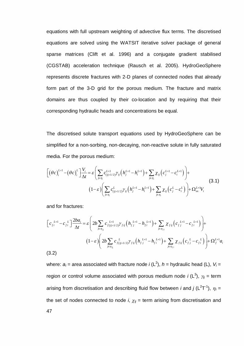
47

equations with full upstream weighting of advective flux terms. The discretised

equations are solved using the WATSIT iterative solver package of general

sparse matrices (Clift et al. 1996) and a conjugate gradient stabilised

(CGSTAB) acceleration technique (Rausch et al. 2005). HydroGeoSphere

represents discrete fractures with 2-D planes of connected nodes that already

form part of the 3-D grid for the porous medium. The fracture and matrix

domains are thus coupled by their co-location and by requiring that their

corresponding hydraulic heads and concentrations be equal.

The discretised solute transport equations used by HydroGeoSphere can be

simplified for a non-sorbing, non-decaying, non-reactive solute in fully saturated

media. For the porous medium:

1 1 1 1 1 11/ 2

1 1 11/ 21

i i

i i

L L L L L L Liij j i ij j iiji i

j j

L L L L L Lij j i ij j i ex iij

j j

Vc c c h h c ct

c h h c c V

(3.1)

and for fractures:

1 1 1 1 1 11/ 2

1 1 11/ 2

2 2

1 2

f f ii

f f ii

L L L L L L Lif i f i f f ij f j f i f ij f j f iij

j j

L L L L L Lf f ij f j f i f ij f j f i f iij

j j

bac c b c h h c ct

b c h h c c a

(3.2)

where: ai = area associated with fracture node i (L2), h = hydraulic head (L), Vi =

region or control volume associated with porous medium node i (L3), ij = term

arising from discretisation and describing fluid flow between i and j (L2T-1), i =

the set of nodes connected to node i, ij = term arising from discretisation and

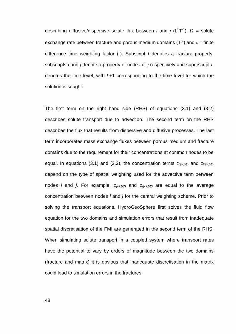
48

describing diffusive/dispersive solute flux between i and j (L3T-1), = solute

exchange rate between fracture and porous medium domains (T-1) and = finite

difference time weighting factor (-). Subscript f denotes a fracture property,

subscripts i and j denote a property of node i or j respectively and superscript L

denotes the time level, with L+1 corresponding to the time level for which the

solution is sought.

The first term on the right hand side (RHS) of equations (3.1) and (3.2)

describes solute transport due to advection. The second term on the RHS

describes the flux that results from dispersive and diffusive processes. The last

term incorporates mass exchange fluxes between porous medium and fracture

domains due to the requirement for their concentrations at common nodes to be

equal. In equations (3.1) and (3.2), the concentration terms c(ij+1/2) and cf(ij+1/2)

depend on the type of spatial weighting used for the advective term between

nodes i and j. For example, c(ij+1/2) and cf(ij+1/2) are equal to the average

concentration between nodes i and j for the central weighting scheme. Prior to

solving the transport equations, HydroGeoSphere first solves the fluid flow

equation for the two domains and simulation errors that result from inadequate

spatial discretisation of the FMI are generated in the second term of the RHS.

When simulating solute transport in a coupled system where transport rates

have the potential to vary by orders of magnitude between the two domains

(fracture and matrix) it is obvious that inadequate discretisation in the matrix

could lead to simulation errors in the fractures.

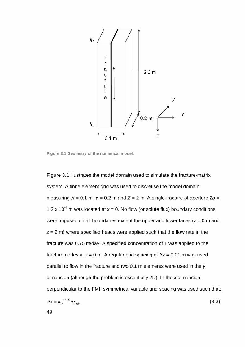
49

Figure 3.1 Geometry of the numerical model.

Figure 3.1 illustrates the model domain used to simulate the fracture-matrix

system. A finite element grid was used to discretise the model domain

measuring X = 0.1 m, Y = 0.2 m and Z = 2 m. A single fracture of aperture 2b =

1.2 x 10-4 m was located at x = 0. No flow (or solute flux) boundary conditions

were imposed on all boundaries except the upper and lower faces (z = 0 m and

z = 2 m) where specified heads were applied such that the flow rate in the

fracture was 0.75 m/day. A specified concentration of 1 was applied to the

fracture nodes at z = 0 m. A regular grid spacing of z = 0.01 m was used

parallel to flow in the fracture and two 0.1 m elements were used in the y

dimension (although the problem is essentially 2D). In the x dimension,

perpendicular to the FMI, symmetrical variable grid spacing was used such that:

minn

x xmx )1( (3.3)

50

where: x = grid spacing in the x direction (L), mx = grid spacing multiplier in the

x direction (-), n = integer element counter where element number 1 borders the

fracture centre (-) and xmin = the minimum element size occurring at n = 1 (L).

Spatial discretisation is often conducted in accordance with the grid Peclet

number:

vDzv

Peg ' (3.4)

As diffusion is typically much smaller than mechanical dispersion (D’ << |v|)

Peg can be simplified to z/ . Depending on the numerical scheme used the

necessary Peclet criterion will vary. However, for numerical stability it is usually

recommended that Peg be less than around 4 (Anderson and Woessner 1992)

up to as high as 10 (Huyakorn and Pinder 1983) when central weighting of the

advective term is used, which is the case for the simulations presented here.

For the chosen grid, Peg is 0.0132 along the fracture. As flow only occurs in the

z direction, Peg is not applicable for the other dimensions.

Temporal discretisation was conducted using HydroGeoSphere’s variable time-

stepping procedure with a Crank-Nicolson implicit finite difference scheme in

time, with = 0.5 in equations (3.1) and (3.2). Once a solution at time L is found,

the next time-step is determined by:

LL

iL

i

maxL tcc

ct1

1

max (3.5)

where cmax = specified maximum change in concentration desired in a time-step

and ci = calculated concentration at node i. This procedure allows the model to

51

increase time-steps when there are only small changes in concentration and

similarly reduce them when rapid changes occur. Thus computation time is

reduced without decreasing numerical accuracy. This study used a very small

initial time-step of 0.01 s and a target concentration change per time-step of

cmax = 0.01. A maximum time-step of 1000 s and maximum time-step multiplier

of 2 were imposed. Model output was generated every 0.4 days for a total

duration of 4 days.

To provide a check on the performance and accuracy of HydroGeoSphere, the

solute transport model MT3DMS (Zheng 1990) was also used to simulate the

system depicted in Figure 3.1. The linked combination of MT3DMS and the

USGS flow code MODFLOW is one of the most commonly used and widely

accepted approaches for modelling flow and solute transport in the subsurface.

In the majority of cases, this combination of models is used to simulate flow and

transport in fractured media utilising the EPM approach, however it is fully

capable of simulating a discrete fracture formulation at very fine grid spacings.

The problem was solved using a third order accurate total variation diminishing

(TVD) scheme. An identical model domain was used for the MT3DMS

simulations. Discretisation in the y and z directions was identical to that used in

HydroGeoSphere. Discretisation perpendicular to the fracture was slightly

different as MT3DMS uses a block-centred rather than point-centred grid. In all

cases elements of width 2b = 1.2 x 10-4 m and 100 % porosity were used for the

fracture. The minimum discretisation in the matrix ( xmin) was varied and a grid

multiplier of 1.5 was used. An initial time-step of 0.001 s and a time-step

multiplier of 1.1 were used with a maximum time-step of 100 s.

52

Model parameters for HydroGeoSphere and MT3DMS simulations were chosen

to match those used by Tang et al. (1981) who in turn successfully replicated

the earlier numerical results of Grisak and Pickens (1980). Those were 2b = 1.2

x 10-4 m, D’ = 10-6, 10-7, 10-8, 10-9, 10-10 and 0 cm2s-1, v = 0.75 mday-1, = 0.76

m and = 0.35. The range of diffusion coefficients covers typical values for free

diffusion in water (10-6 cm2s-1) through to diffusion in tortuous rock (10-11 cm2s-

1). In addition, a matrix hydraulic conductivity of 10-50 ms-1 was used to ensure

water flow in the matrix was negligible. Model parameters, grid and time-

stepping specifications are summarised in Table 3.1. Grids employing different

spatial discretisation were used to model the Tang et al. (1981) problem. Unless

otherwise stated xmin = 2b = 1.2 x 10-4 m and mx = 2.

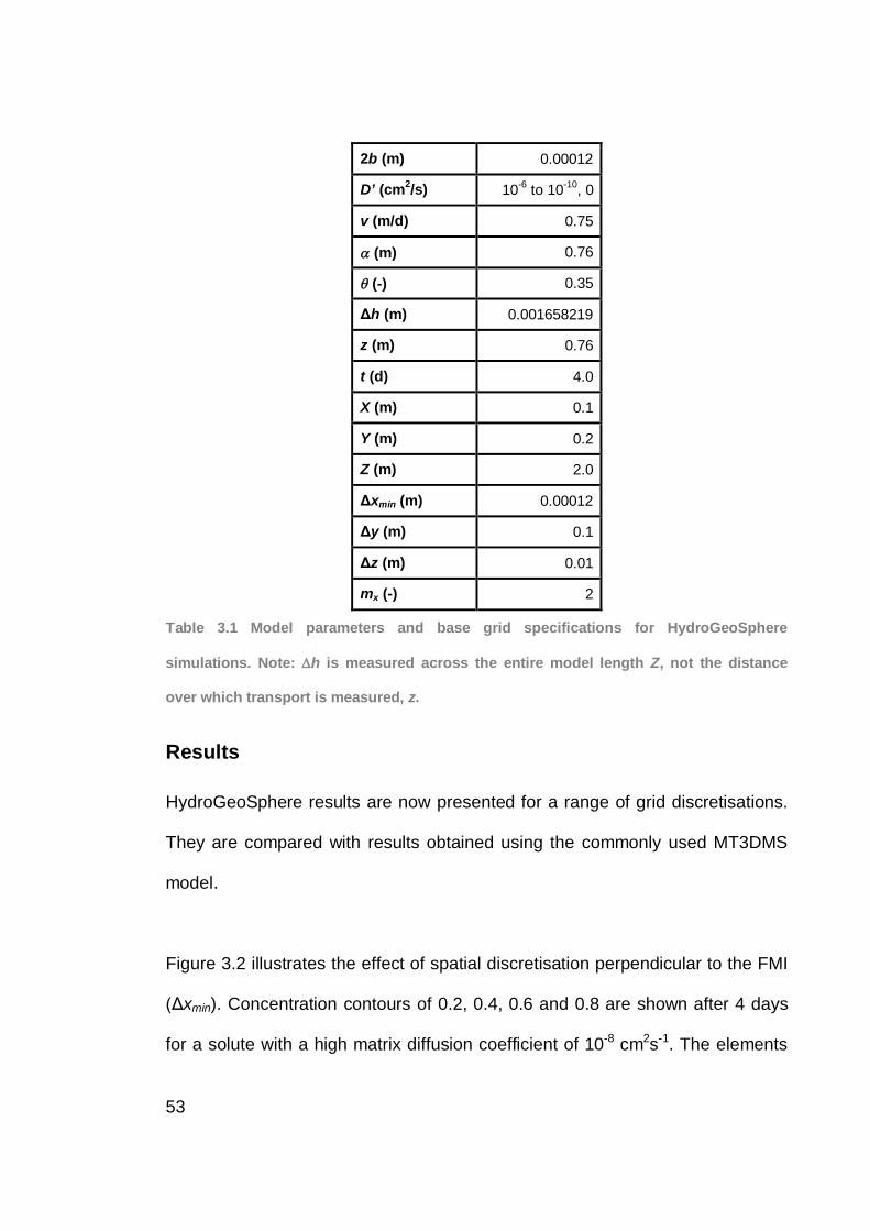
53

2b (m) 0.00012

D’ (cm2/s) 10-6 to 10-10, 0

v (m/d) 0.75

(m) 0.76

(-) 0.35

h (m) 0.001658219

z (m) 0.76

t (d) 4.0

X (m) 0.1

Y (m) 0.2

Z (m) 2.0

xmin (m) 0.00012

y (m) 0.1

z (m) 0.01

mx (-) 2

Table 3.1 Model parameters and base grid specifications for HydroGeoSphere

simulations. Note: h is measured across the entire model length Z, not the distance

over which transport is measured, z.

Results

HydroGeoSphere results are now presented for a range of grid discretisations.

They are compared with results obtained using the commonly used MT3DMS

model.

Figure 3.2 illustrates the effect of spatial discretisation perpendicular to the FMI

xmin). Concentration contours of 0.2, 0.4, 0.6 and 0.8 are shown after 4 days

for a solute with a high matrix diffusion coefficient of 10-8 cm2s-1. The elements

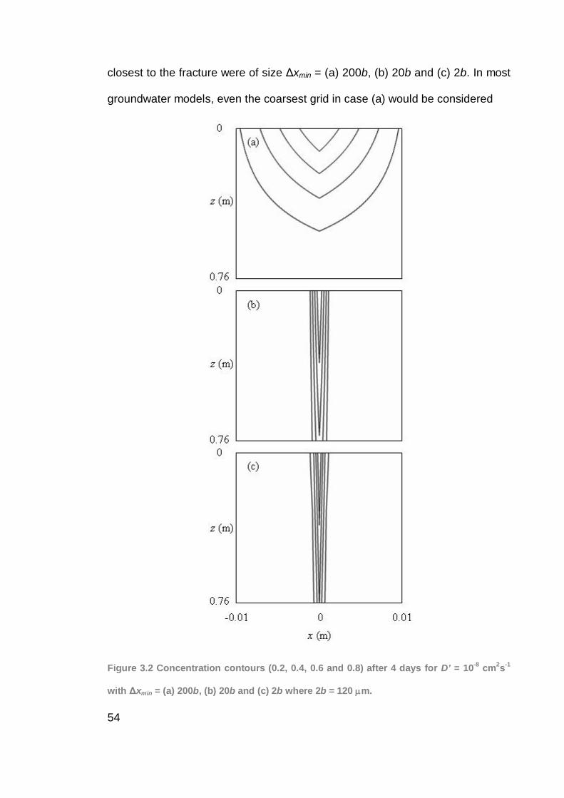
54

closest to the fracture were of size xmin = (a) 200b, (b) 20b and (c) 2b. In most

groundwater models, even the coarsest grid in case (a) would be considered

Figure 3.2 Concentration contours (0.2, 0.4, 0.6 and 0.8) after 4 days for D’ = 10-8 cm2s-1

with xmin = (a) 200b, (b) 20b and (c) 2b where 2b = 120 m.

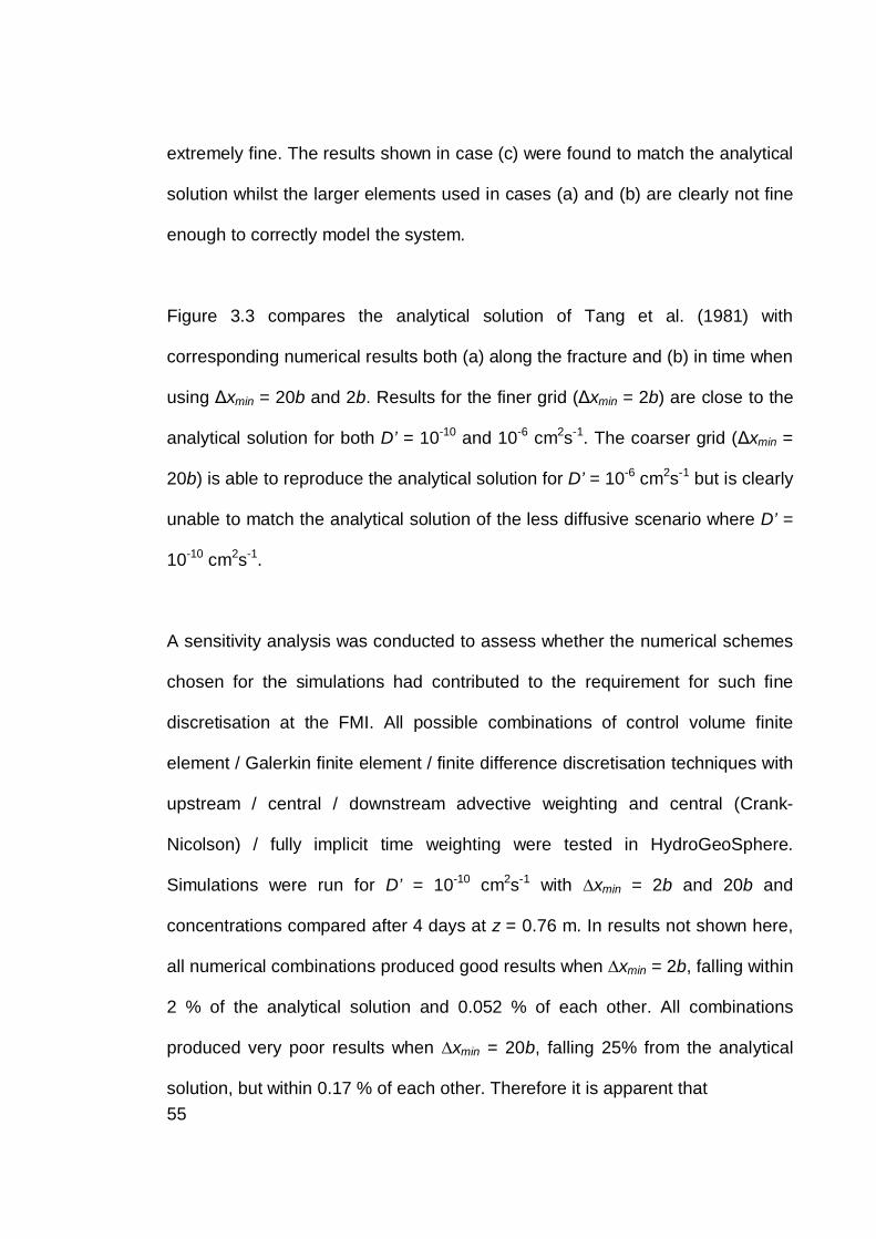
55

extremely fine. The results shown in case (c) were found to match the analytical

solution whilst the larger elements used in cases (a) and (b) are clearly not fine

enough to correctly model the system.

Figure 3.3 compares the analytical solution of Tang et al. (1981) with

corresponding numerical results both (a) along the fracture and (b) in time when

using xmin = 20b and 2b. Results for the finer grid ( xmin = 2b) are close to the

analytical solution for both D’ = 10-10 and 10-6 cm2s-1. The coarser grid ( xmin =

20b) is able to reproduce the analytical solution for D’ = 10-6 cm2s-1 but is clearly

unable to match the analytical solution of the less diffusive scenario where D’ =

10-10 cm2s-1.

A sensitivity analysis was conducted to assess whether the numerical schemes

chosen for the simulations had contributed to the requirement for such fine

discretisation at the FMI. All possible combinations of control volume finite

element / Galerkin finite element / finite difference discretisation techniques with

upstream / central / downstream advective weighting and central (Crank-

Nicolson) / fully implicit time weighting were tested in HydroGeoSphere.

Simulations were run for D’ = 10-10 cm2s-1 with xmin = 2b and 20b and

concentrations compared after 4 days at z = 0.76 m. In results not shown here,

all numerical combinations produced good results when xmin = 2b, falling within

2 % of the analytical solution and 0.052 % of each other. All combinations

produced very poor results when xmin = 20b, falling 25% from the analytical

solution, but within 0.17 % of each other. Therefore it is apparent that

56

Figure 3.3 Comparison of the HydroGeoSphere concentrations for xmin = 20b and 2b

with the analytical solution for D’ = 10-10 and 10-6 cm2s-1: (a) concentration along the

fracture at t = 4 days and (b) concentration with time at z = 0.76 m.

regardless of the numerical methods used to calculate the solution in

HydroGeoSphere, a very fine grid is required at the FMI to match the analytical

solution under the physical conditions simulated in the model.

MT3DMS results presented in Figure 3.4 confirm that the HydroGeoSphere

results are not a code specific phenomenon. It is immediately obvious that both

models require extremely fine discretisation to match analytical results for low

57

diffusion coefficients but that less strict discretisation requirements can be

tolerated for a higher diffusion coefficient. It is also of interest to note the

performance of MT3DMS when the element size immediately adjacent to the

fracture is 200b, which is still a fine grid compared to that used for most field

scale simulations. The predicted migration of the solute through the fracture is

severely underestimated, in particular for the case with lower diffusion (D’ = 10-

10 cm2s-1). Erroneously, the value of the diffusion coefficient itself has little effect

on the model prediction, further emphasising the importance of fine grid

discretisation in discrete fracture modelling. Given the results for the range of

numerical schemes tested in HydroGeoSphere, plus the TVD scheme used in

MT3DMS, it appears that the requirement for fine gridding at the FMI under

conditions of low diffusion is neither a phenomenon of the codes nor the

numerical schemes utilised in them.

Figure 3.5 shows simulated concentrations normalised by their corresponding

analytical values as a function of xmin/2b. It is readily apparent that highly

diffusive cases are able to achieve better agreement between numerical and

analytical solutions for larger element sizes but that for low diffusivity cases,

xmin/2b 1 is required for a match. All cases converge once xmin/2b reduces

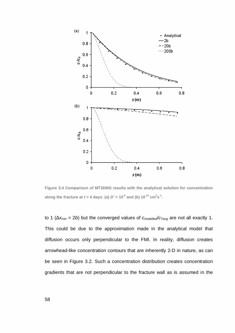
58

Figure 3.4 Comparison of MT3DMS results with the analytical solution for concentration

along the fracture at t = 4 days: (a) D’ = 10-6 and (b) 10-10 cm2s-1.

to 1 ( xmin = 2b) but the converged values of cmodelled/cTang are not all exactly 1.

This could be due to the approximation made in the analytical model that

diffusion occurs only perpendicular to the FMI. In reality, diffusion creates

arrowhead-like concentration contours that are inherently 2-D in nature, as can

be seen in Figure 3.2. Such a concentration distribution creates concentration

gradients that are not perpendicular to the fracture wall as is assumed in the

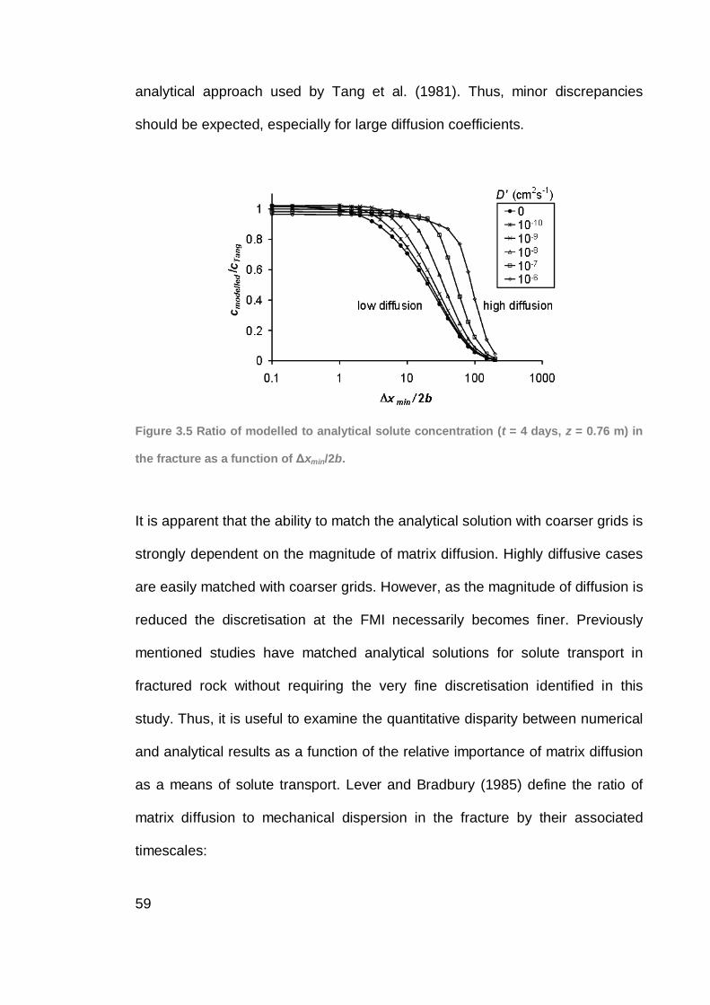
59

analytical approach used by Tang et al. (1981). Thus, minor discrepancies

should be expected, especially for large diffusion coefficients.

Figure 3.5 Ratio of modelled to analytical solute concentration (t = 4 days, z = 0.76 m) in

the fracture as a function of xmin/2b.

It is apparent that the ability to match the analytical solution with coarser grids is

strongly dependent on the magnitude of matrix diffusion. Highly diffusive cases

are easily matched with coarser grids. However, as the magnitude of diffusion is

reduced the discretisation at the FMI necessarily becomes finer. Previously

mentioned studies have matched analytical solutions for solute transport in

fractured rock without requiring the very fine discretisation identified in this

study. Thus, it is useful to examine the quantitative disparity between numerical

and analytical results as a function of the relative importance of matrix diffusion

as a means of solute transport. Lever and Bradbury (1985) define the ratio of

matrix diffusion to mechanical dispersion in the fracture by their associated

timescales:

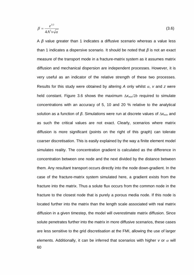
60

vAz2

23

4 (3.6)

A value greater than 1 indicates a diffusive scenario whereas a value less

than 1 indicates a dispersive scenario. It should be noted that is not an exact

measure of the transport mode in a fracture-matrix system as it assumes matrix

diffusion and mechanical dispersion are independent processes. However, it is

very useful as an indicator of the relative strength of these two processes.

Results for this study were obtained by altering A only whilst , v and z were

held constant. Figure 3.6 shows the maximum xmin/2b required to simulate

concentrations with an accuracy of 5, 10 and 20 % relative to the analytical

solution as a function of . Simulations were run at discrete values of xmin and

as such the critical values are not exact. Clearly, scenarios where matrix

diffusion is more significant (points on the right of this graph) can tolerate

coarser discretisation. This is easily explained by the way a finite element model

simulates reality. The concentration gradient is calculated as the difference in

concentration between one node and the next divided by the distance between

them. Any resultant transport occurs directly into the node down-gradient. In the

case of the fracture-matrix system simulated here, a gradient exists from the

fracture into the matrix. Thus a solute flux occurs from the common node in the

fracture to the closest node that is purely a porous media node. If this node is

located further into the matrix than the length scale associated with real matrix

diffusion in a given timestep, the model will overestimate matrix diffusion. Since

solute penetrates further into the matrix in more diffusive scenarios, these cases

are less sensitive to the grid discretisation at the FMI, allowing the use of larger

elements. Additionally, it can be inferred that scenarios with higher v or will

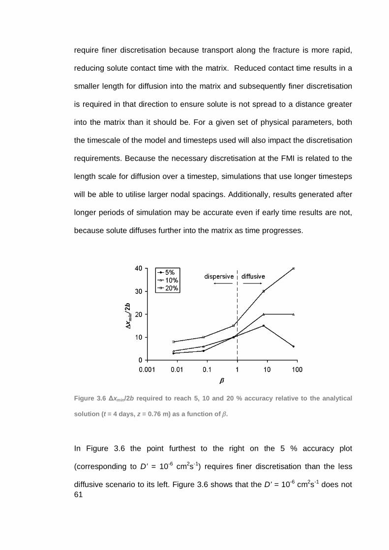
61

require finer discretisation because transport along the fracture is more rapid,

reducing solute contact time with the matrix. Reduced contact time results in a

smaller length for diffusion into the matrix and subsequently finer discretisation

is required in that direction to ensure solute is not spread to a distance greater

into the matrix than it should be. For a given set of physical parameters, both

the timescale of the model and timesteps used will also impact the discretisation

requirements. Because the necessary discretisation at the FMI is related to the

length scale for diffusion over a timestep, simulations that use longer timesteps

will be able to utilise larger nodal spacings. Additionally, results generated after

longer periods of simulation may be accurate even if early time results are not,

because solute diffuses further into the matrix as time progresses.

Figure 3.6 xmin/2b required to reach 5, 10 and 20 % accuracy relative to the analytical

solution (t = 4 days, z = 0.76 m) as a function of .

In Figure 3.6 the point furthest to the right on the 5 % accuracy plot

(corresponding to D’ = 10-6 cm2s-1) requires finer discretisation than the less

diffusive scenario to its left. Figure 3.6 shows that the D’ = 10-6 cm2s-1 does not

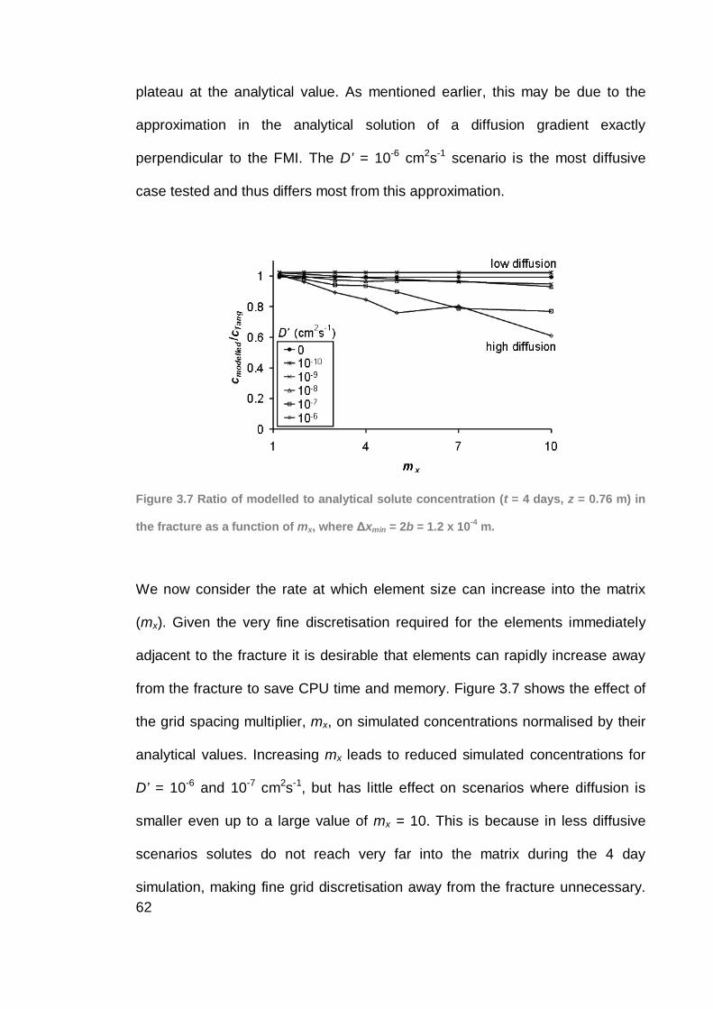
62

plateau at the analytical value. As mentioned earlier, this may be due to the

approximation in the analytical solution of a diffusion gradient exactly

perpendicular to the FMI. The D’ = 10-6 cm2s-1 scenario is the most diffusive

case tested and thus differs most from this approximation.

Figure 3.7 Ratio of modelled to analytical solute concentration (t = 4 days, z = 0.76 m) in

the fracture as a function of mx, where xmin = 2b = 1.2 x 10-4 m.

We now consider the rate at which element size can increase into the matrix

(mx). Given the very fine discretisation required for the elements immediately

adjacent to the fracture it is desirable that elements can rapidly increase away

from the fracture to save CPU time and memory. Figure 3.7 shows the effect of

the grid spacing multiplier, mx, on simulated concentrations normalised by their

analytical values. Increasing mx leads to reduced simulated concentrations for

D’ = 10-6 and 10-7 cm2s-1, but has little effect on scenarios where diffusion is

smaller even up to a large value of mx = 10. This is because in less diffusive

scenarios solutes do not reach very far into the matrix during the 4 day

simulation, making fine grid discretisation away from the fracture unnecessary.

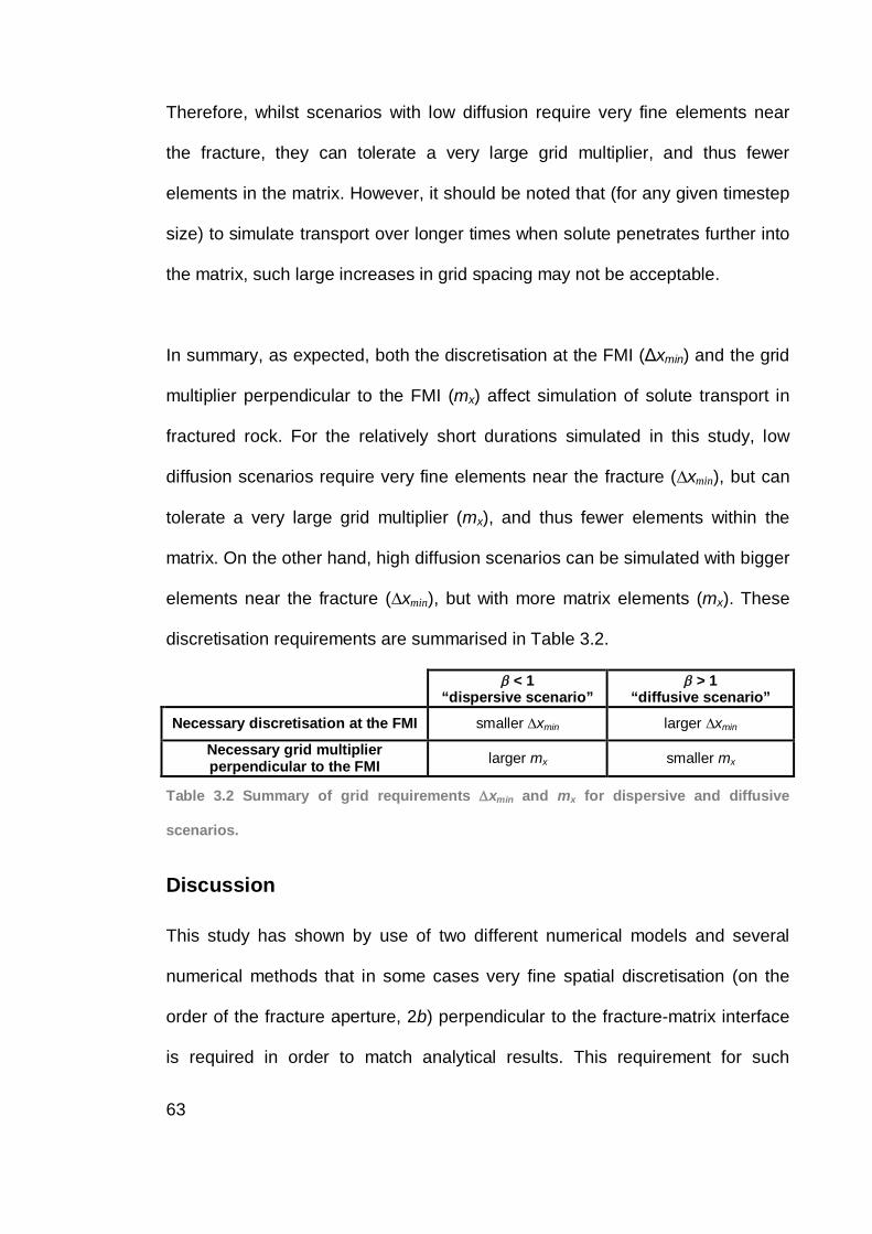
63

Therefore, whilst scenarios with low diffusion require very fine elements near

the fracture, they can tolerate a very large grid multiplier, and thus fewer

elements in the matrix. However, it should be noted that (for any given timestep

size) to simulate transport over longer times when solute penetrates further into

the matrix, such large increases in grid spacing may not be acceptable.

In summary, as expected, both the discretisation at the FMI ( xmin) and the grid

multiplier perpendicular to the FMI (mx) affect simulation of solute transport in

fractured rock. For the relatively short durations simulated in this study, low

diffusion scenarios require very fine elements near the fracture ( xmin), but can

tolerate a very large grid multiplier (mx), and thus fewer elements within the

matrix. On the other hand, high diffusion scenarios can be simulated with bigger

elements near the fracture ( xmin), but with more matrix elements (mx). These

discretisation requirements are summarised in Table 3.2.

< 1 “dispersive scenario”

> 1 “diffusive scenario”

Necessary discretisation at the FMI smaller xmin larger xmin

Necessary grid multiplier perpendicular to the FMI larger mx smaller mx

Table 3.2 Summary of grid requirements xmin and mx for dispersive and diffusive

scenarios.

Discussion

This study has shown by use of two different numerical models and several

numerical methods that in some cases very fine spatial discretisation (on the

order of the fracture aperture, 2b) perpendicular to the fracture-matrix interface

is required in order to match analytical results. This requirement for such

64

extremely fine discretisation has not been reported by previous authors. The

results indicate that scenarios where matrix diffusion is relatively high (i.e.

slower water flow, higher porosity or diffusion coefficient, smaller aperture,

longer times) do not require such small elements. On the other hand scenarios

with low matrix diffusion require extremely fine grids (see Table 3.2). The

aforementioned studies of Sudicky and McLaren (1992) and Cook et al. (2005)

in which elements 250 times the fracture aperture were used to match the

analytical solution of Sudicky and Frind (1982) were conducted using

parameters which equate to values of 0.143 and 885 respectively. These

represent a slightly dispersive scenario and a highly diffusive scenario and

combined with their long simulation periods of around 27.5 and 55 years in the

case of Sudicky and McLaren (1992) and approximately 50 years for Cook et al.

(2005), explain why they were able to use such large elements without

encountering significant errors.

Thus, in many cases solute transport may be simulated accurately without

discretisation on the order of the fracture aperture. However, when simulating

scenarios involving high water velocity (e.g. forced gradient tracer tests), small

diffusion coefficients (e.g. large compounds such as Uranium), low matrix

porosity or very large fractures, simulations are prone to error and a rigorous

sensitivity analysis of solutions to grid discretisation is warranted.

As a consequence of the inherent discretisation required for some practical

scenarios, the use of discrete fracture network models in the simulation of

catchment-scale phenomena may be severely limited by computing capacity.

65

With current computing capabilities, models requiring discretisation on the scale

of the fracture aperture will be limited to incorporation of very few fractures

and/or small scale model dimensions.

Conclusions

This study has examined the spatial discretisation required perpendicular to the

fracture-matrix interface (FMI) in a discrete fracture model in order to

demonstrate how simulation accuracy and required discretisation are influenced

by the diffusive-dispersive nature of the problem being considered. Comparison

with the analytical solution of Tang et al. (1981) has indicated:

1. Finite difference and element grids need to be designed according to the

relative dominance of advection and dispersion in the fracture to diffusion in

the matrix.

2. Diffusive scenarios ( > 1) tolerate larger elements close to the FMI (large

xmin) but require the growth of matrix elements moving away from the

fracture to be gradual (small mx), a result not reported in previous literature.

3. Dispersive scenarios ( < 1) require small elements close to the FMI (small

xmin), but are able to employ larger matrix elements (large mx) for relatively

short timescales, before solute penetrates far into the matrix, a result not

reported in previous literature.

4. Results were compared from a wide range of numerical schemes and two

different numerical codes. The requirement for fine discretisation at the FMI

was found to be neither a phenomenon of the codes nor the numerical

schemes used within them.

66

5. Minor discrepancies between numerical and analytical results were

observed, especially for diffusive scenarios. These are assumed to be due

to the assumption made in the analytical solution that matrix diffusion occurs

only perpendicular to the FMI, but which is inherently 2-D in the numerical

framework considered here.

6. Whilst it has previously been reported that fine discretisation is required to

simulate solute transport in discretely fractured media, this study has

quantified the relationship between xmin and showing that the grid

discretisation required for low matrix diffusion scenarios can be on the order

of the size of the fracture aperture ( xmin 2b). This necessary grid spacing

requirement is extremely fine and has not been reported previously in the

literature.

7. Whilst the discretisation requirements at the FMI and in the adjacent matrix

are related to the physical parameters of the system being modelled (eg D’,

v, z), they are also tied to the timescales used for individual timesteps and

overall model duration.

The results of this study clearly indicate that caution must be taken when

modelling solute transport in discrete fracture systems using a numerical model.

Careful attention must be given to the diffusive/dispersive ratio in the system

under consideration. Critically, the results of this study provide guidance on the

choice of xmin and mx that should be employed for the varying cases of

diffusive/dispersive effects in the physical system under consideration. These

results are demonstrative and indicative only and we wish to exercise some

caution in overgeneralising results here. However, it is abundantly clear that a

67

sensitivity analysis must be conducted to determine the precise spatial and

temporal discretisation required in any given model of solute transport in

fractured porous media.

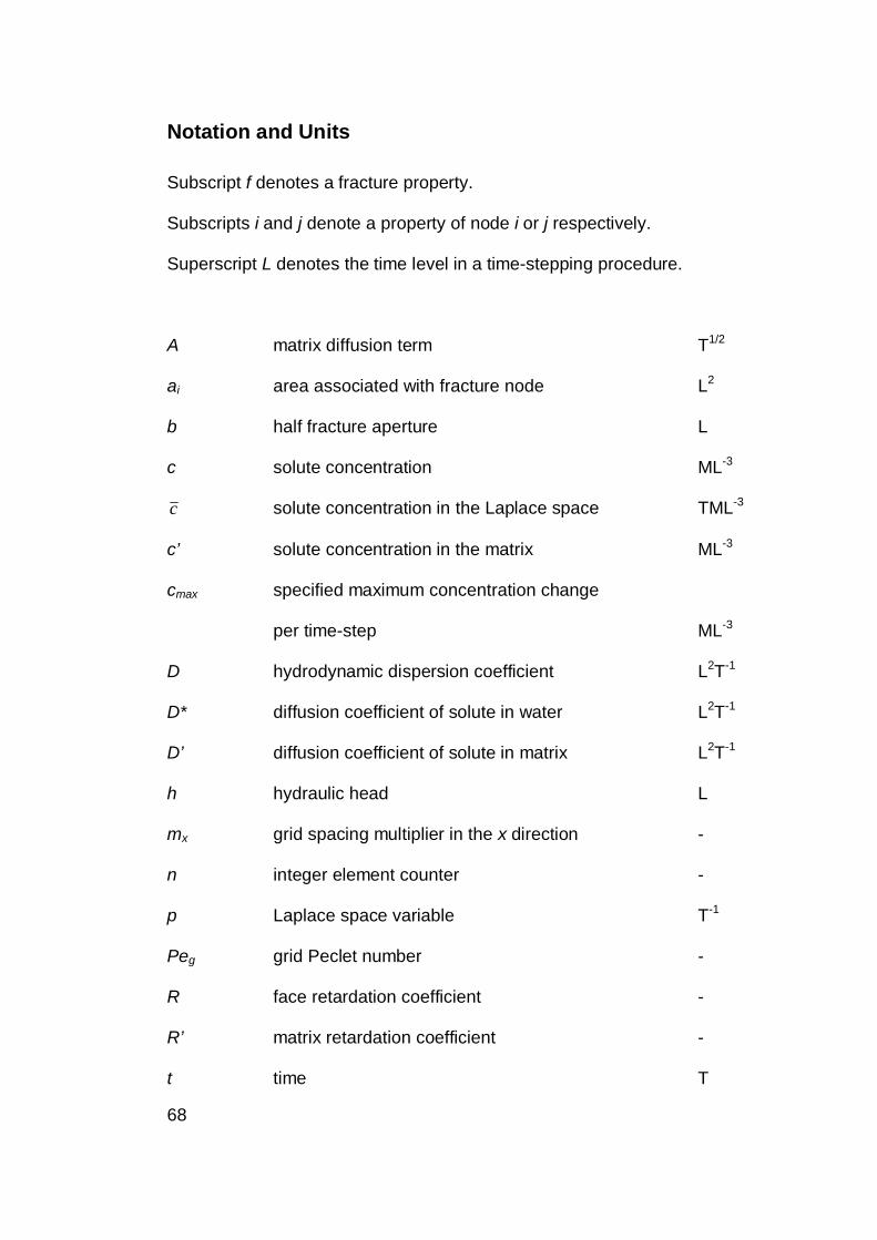
68

Notation and Units

Subscript f denotes a fracture property.

Subscripts i and j denote a property of node i or j respectively.

Superscript L denotes the time level in a time-stepping procedure.


ai area associated with fracture node L2



c solute concentration in the Laplace space TML-3


cmax specified maximum concentration change

per time-step ML-3




h hydraulic head L

mx grid spacing multiplier in the x direction -

n integer element counter -

p Laplace space variable T-1

Peg grid Peclet number -



t time T

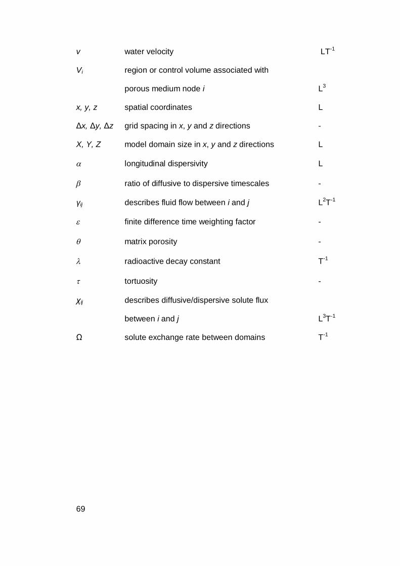
69


Vi region or control volume associated with

porous medium node i L3

x, y, z spatial coordinates L

x, y, z grid spacing in x, y and z directions -

X, Y, Z model domain size in x, y and z directions L


ratio of diffusive to dispersive timescales -

ij describes fluid flow between i and j L2T-1

finite difference time weighting factor -

matrix porosity -


tortuosity -

ij describes diffusive/dispersive solute flux

between i and j L3T-1

solute exchange rate between domains T-1

70

References

Anderson, M. P. and W. W. Woessner. 1992. Applied Groundwater Modeling:

Simulation of Flow and Advective Transport, San Diego: Academic Press, Inc.

Chan, T., N. W. Scheier and V. Guvanasen. 1999a. MOTIF Version 3.2 Theory

Manual, 06819-REP-01200-0091-R00. Toronto: Nuclear Waste Management

Division, Ontario Power Generation Inc.

Chan, T., N. W. Scheier and F. W. Stanchell. 1999b. MOTIF Code Version 3.2

User's Manual, 06819-REP-01200-0090-R00. Toronto: Nuclear Waste

Management Division, Ontario Power Generation Inc.

Clift, S. S., E. F. D'Azevedo, P. A. Forsyth and J. R. Knightly. 1996. WATSIT-1

and WATSIT-B Waterloo Sparse Iterative Matrix Solvers. User's Guide with

Developer Notes for Version 2.0.0.

Cook, P. G., A. J. Love, N. I. Robinson and C. T. Simmons. 2005. Groundwater

ages in fractured rock aquifers. Journal of Hydrology 308: 284-301.

Diodato, D. M. 1994. A Compendium of Fracture Flow Models, Argonne:

Argonne National Laboratory.

England, R. L., N. W. Kline, K. J. Ekblad and R. G. Baca. 1986. MAGNUM-2D

Computer Code: User's Guide, RHO-CR-143P. Rockwell Hanford Operations.

Graf, T. and R. Therrien. 2005. Variable-density groundwater flow and solute

transport in porous media containing nonuniform discrete fractures. Advances in

Water Resources 28, no. 12: 1351-1367.

Grisak, G. E. and J. F. Pickens. 1980. Solute transport through fractured media

1. the effect of matrix diffusion. Water Resources Research 16, no. 4: 719-730.

71

HSI-GeoTrans. 2000. Theory and Implementation for SWIFT for Windows: The

Sandia Waste-Isolation Flow and Transport Model for Fractured Media, Sterling:

HSI GeoTrans.

Huyakorn, P. S. and G. F. Pinder. 1983. Computational Methods in Subsurface

Flow, Orlando: Academic Press, Inc.

Lever, D. A. and M. H. Bradbury. 1985. Rock-matrix diffusion and its

implications for radionuclide migration. Mineralogical Magazine 49: 245-254.

Neuman, S. P. 2005. Trends, prospects and challenges in quantifying flow and

transport through fractured rocks. Hydrogeology Journal 13, no. 1: 124-147.

Piessens, R. and R. Huysmans. 1984. Algorithm 619. Automatic numerical


Transactions on Mathematical Software 10: 348-353.

Rausch, R., W. Schafer, R. Therrien and C. Wagner. 2005. Solute Transport

Modelling: An Introduction to Models and Solution Strategies, Stuttgart:

Borntraeger.

Reynolds, D. A. and B. H. Kueper. 2002. Numerical examination of the factors

controlling DNAPL migration through a single fracture. Ground Water 40, no. 4:

368-377.

Robinson, N. I. and J. M. Sharp. 1997. Analytical solution for solute transport in

a finite set of parallel fractures with matrix diffusion, CMIS C23/97. Adelaide:

CSIRO.

Runchal, A. 2002. PORFLOW User's Manual, Version 5, Analytic &

Computational Research, Inc.

72

Slough, K. J., E. A. Sudicky and P. A. Forsyth. 1999. Grid refinement for

modeling multiphase flow in discretely fractured porous media. Advances in

Water Resources 23, no. 3: 261-269.

Sudicky, E. A. and E. O. Frind. 1982. Contaminant transport in fractured porous

media: analytical solutions for a system of parallel fractures. Water Resources

Research 18, no. 6: 1634-1642.

Sudicky, E. A. and R. G. McLaren. 1992. The Laplace transform Galerkin

technique for large-scale simulation of mass transport in discretely fractured

porous formations. Water Resources Research 28, no. 2: 499-514.

Sudicky, E. A. and R. G. McLaren. 1998. FRACTRAN User's Guide. An Efficient

Simulator for Two-Dimensional, Saturated Groundwater Flow and Solute

Transport in Porous or Discretely-Fractured Porous Formations, Ontario:

Groundwater Simulations Group, Waterloo Centre for Groundwater Research,

University of Waterloo.

Tang, D. H., E. O. Frind and E. A. Sudicky. 1981. Contaminant transport in


Resources Research 17, no. 3: 555-564.

Therrien, R. and E. A. Sudicky. 1996. Three-dimensional analysis of variably-

saturated flow and solute transport in discretely-fractured porous media. Journal

of Contaminant Hydrology 23, no. 1-2: 1-44.

Therrien, R., E. A. Sudicky, R. G. McLaren and S. M. Panday. 2005.

HydroGeoSphere: A three-dimensional numerical model describing fully-

integrated subsurface and surface flow and solute transport. User's Guide,

Waterloo, Canada: Groundwater Simulations Group.

73

Travis, B. J. and K. H. Birdsell. 1991. TRACR3D: A Model of Flow and

Transport in Porous Media, Model Description and User's Manual, Los Alamos

National Laboratory.

VanderKwaak, J. E. and E. A. Sudicky. 1996. Dissolution of non-aqueous-

phase liquids and aqueous-phase contaminant transport in discretely-fractured

porous media. Journal of Contaminant Hydrology 23, no. 1-2: 45-68.

Zheng, C. 1990. MT3D: A modular three-dimensional transport model for

simulation of advection, dispersion and chemical reactions of contaminants in

groundwater systems, Rockville, USA: S.S. Papadopulos and Associates Inc.

74

Chapter 4: Conceptual model choice for dipole tracer

tests in fractured rock

Abstract

Applied tracer tests provide a means to estimate fracture and matrix parameters

that determine solute transport in fractured rock. Dipole tracer tests utilise an

injection-extraction well pair to create a forced hydraulic gradient, allowing tests

to be conducted more rapidly than natural gradient tests. Tracer breakthrough is

analysed using an analytical model to find the parameters that generate the

best fit to the data. This study explores the differing interpretation that can be

drawn from a tracer test when analysed with two different models; one

assuming a dipole, the other a linear flow field. The analytical solution of Tang

et al. (1981) is used to model a 1-D flow field and a multiple streamline

summation of the same model is used to represent transport in a dipole flow

field. The two models are able to produce almost identical breakthrough curves

for a range of scenarios. Comparison of the parameters required to create

matching breakthrough curves demonstrates the non-uniqueness of the 1-D

and dipole interpretations, resulting in large parameter uncertainty. Considering

that neither of the conceptual models incorporates the complexity of a real

fracture network, it is expected that analytically interpreted parameters may be

as different, or more different from reality as they are from those interpreted with

a different analytical model. Given the complex nature of fractured rock systems

and the many unknown fracture and matrix properties involved therein, this

75

study highlights the benefit of incorporating multiple conceptual models in the

analyses of dipole tracer tests conducted in fractured rock.

Introduction

Dipole tracer tests are used as an in-situ means of characterising the solute

transport properties of fractured rock systems. A dipole tracer test is conducted

by applying tracer to the injection well of an injection-extraction well pair and

monitoring its concentration in the extraction well. The resultant breakthrough

curve is analysed with an analytical model to determine the parameters that

generate the best fit to the observed data.

Grove and Beetem (1971) outlined a method for modelling a 2-D dipole of equal

pole strength (as would occur in a fracture of infinite extent with smooth parallel

walls). The approach is a summation of breakthrough curves from multiple

streamlines. Each streamline has a path length and average flow velocity

dependent on the angle of departure from the injection well. This method has

been widely used to interpret dipole tracer tests conducted in single fractures

(Novakowski, 1988; Novakowski et al., 2004; Novakowski et al., 1985) and in

fracture networks (Himmelsbach et al., 1998; Himmelsbach and Maloszewski,

1992; Sanford et al., 2002; Webster et al., 1970).

Besides the usual experimental error, analyses of dipole tracer tests in fracture

networks are inherently subject to potentially large errors due to the inability of

analytical models to describe the unknown heterogeneity of complex fracture

geometries at appropriate spatial scales. Consequently, the choice of model

76

used to analyse a tracer test is potentially the largest error in the analysis.

Different approaches have been used to explain the long tailing typically

observed in breakthrough curves from fractured rock. In many cases this is

attributed to matrix diffusion. Tracers with differing diffusion coefficients have

been found to produce different breakthrough curves (Jardine et al., 1999;

Maloszewski et al., 1999; Sanford et al., 2002). The analytical models of Grisak

and Pickens (1981), Tang et al. (1981) and Sudicky and Frind (1982)

incorporate matrix diffusion and may be used to obtain transport parameters in

such cases. Other authors (Becker and Shapiro, 2000; Tsang et al., 1991)

attribute tracer tailing to complex transport pathways resulting in tracer

channelling within and between fractures. Becker and Shapiro (2000) presented

identical late-time breakthrough behaviour for tracers with different diffusion

coefficients and claimed this proved that matrix diffusion was not responsible for

the long tailing. Models such as those presented by Maloszewski et al. (1992),

Neretnieks (1983), Rasmuson and Neretnieks (1986) and Tsang and Tsang

(1987) may be used to interpret tracer tailing by channelling. In addition to these

processes, tracer tests conducted in a dipole flow field are subject to long tailing

due to the flow field geometry. With a range of models available for interpreting

tracer tests in fractured rock a unique set of hydrogeologic parameters may be

difficult to identify. As it is often not possible to know which model/s will best

approximate a system, recent studies have begun to compare the analyses of

tracer tests with different models (Akin, 2005; Pfingsten and Soler, 2003).

Typically dipole tracer tests are analysed assuming that a perfect dipole is

attained in the fracture/s. However, laterally finite fractures and variable fracture

77

apertures may channel flow such that infinite dipole flow fields cannot develop

and therefore a 1-D flow model may in fact better describe some systems. 1-D

flow models have also previously been used to interpret dipole tracer tests

where injection and extraction rates are not equal (Pfingsten and Soler, 2003).

In order to demonstrate the potential non-uniqueness that may arise from the

choice of conceptual model used to interpret dipole tracer tests, this study

compares the parameters obtained by two models, one assuming a dipole flow

field and the other a 1-D flow field. The models otherwise incorporate the same

physical processes and parameters. These models are chosen as examples

only in order to demonstrate the principle of non-uniqueness and consequences

for parameter estimation. This study examines the degree of uncertainty in

model parameters that can occur due to conceptual model choice when

interpreting a dipole tracer test conducted in fractured rock. It is demonstrated

that breakthrough curves can be easily fitted with both the dipole and 1-D

analytical models. It is not easy to determine which fit, if any, is superior and

more meaningful. Furthermore the values of the fitting parameters are seen to

be vastly different and this has major implications for subsequent predictions

that may be made using these parameters.

Methods

In order to compare the best-fit parameters yielded by fitting a breakthrough

curve with two different flow models, a dipole flow model was used to create

synthetic breakthrough curves which were subsequently analysed using a 1-D

flow model. The roles of the two models could have been reversed, but the

same conclusions would have been reached. The model used for the 1-D flow

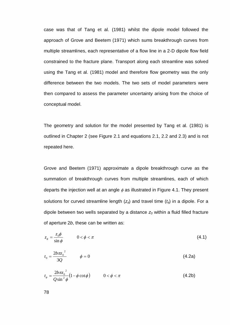
78

case was that of Tang et al. (1981) whilst the dipole model followed the

approach of Grove and Beetem (1971) which sums breakthrough curves from

multiple streamlines, each representative of a flow line in a 2-D dipole flow field

constrained to the fracture plane. Transport along each streamline was solved

using the Tang et al. (1981) model and therefore flow geometry was the only

difference between the two models. The two sets of model parameters were

then compared to assess the parameter uncertainty arising from the choice of

conceptual model.



repeated here.

Grove and Beetem (1971) approximate a dipole breakthrough curve as the

summation of breakthrough curves from multiple streamlines, each of which

departs the injection well at an angle as illustrated in Figure 4.1. They present

solutions for curved streamline length (z ) and travel time (t ) in a dipole. For a

dipole between two wells separated by a distance z0 within a fluid filled fracture

of aperture 2b, these can be written as:

0sin

0zz (4.1)

03

2 20

0 Qzb

t (4.2a)

0cot1sin

22

20

Qzb

t (4.2b)

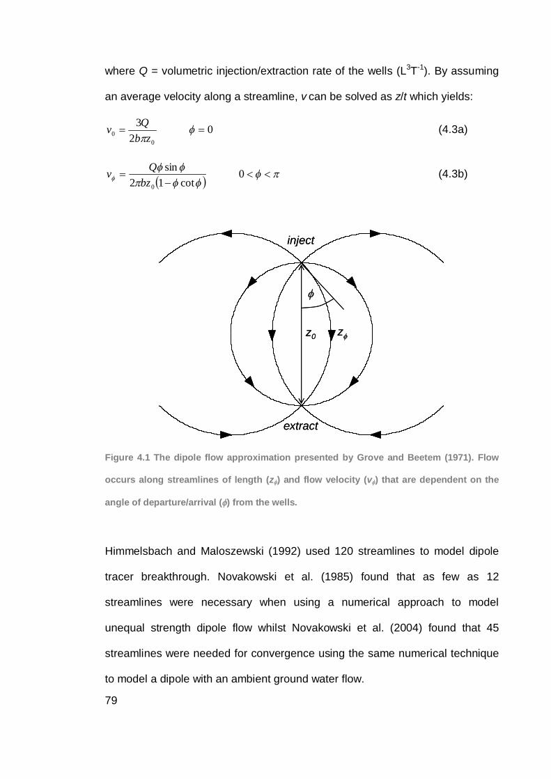
79

where Q = volumetric injection/extraction rate of the wells (L3T-1). By assuming

an average velocity along a streamline, v can be solved as z/t which yields:

02

3

00 zb

Qv (4.3a)

0cot12

sin

0bzQv (4.3b)

z0

inject

extract

zz0

inject

extract

z

Figure 4.1 The dipole flow approximation presented by Grove and Beetem (1971). Flow

occurs along streamlines of length (z ) and flow velocity (v ) that are dependent on the

angle of departure/arrival ( ) from the wells.

Himmelsbach and Maloszewski (1992) used 120 streamlines to model dipole

tracer breakthrough. Novakowski et al. (1985) found that as few as 12

streamlines were necessary when using a numerical approach to model

unequal strength dipole flow whilst Novakowski et al. (2004) found that 45

streamlines were needed for convergence using the same numerical technique

to model a dipole with an ambient ground water flow.

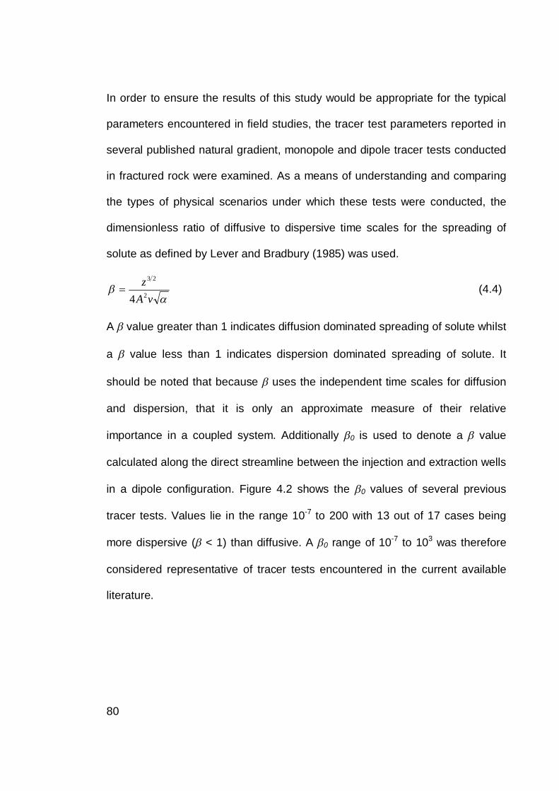
80

In order to ensure the results of this study would be appropriate for the typical

parameters encountered in field studies, the tracer test parameters reported in

several published natural gradient, monopole and dipole tracer tests conducted

in fractured rock were examined. As a means of understanding and comparing

the types of physical scenarios under which these tests were conducted, the

dimensionless ratio of diffusive to dispersive time scales for the spreading of

solute as defined by Lever and Bradbury (1985) was used.

vAz2

23

4 (4.4)

A value greater than 1 indicates diffusion dominated spreading of solute whilst

a value less than 1 indicates dispersion dominated spreading of solute. It

should be noted that because uses the independent time scales for diffusion

and dispersion, that it is only an approximate measure of their relative

importance in a coupled system. Additionally 0 is used to denote a value

calculated along the direct streamline between the injection and extraction wells

in a dipole configuration. Figure 4.2 shows the 0 values of several previous

tracer tests. Values lie in the range 10-7 to 200 with 13 out of 17 cases being

more dispersive ( < 1) than diffusive. A 0 range of 10-7 to 103 was therefore

considered representative of tracer tests encountered in the current available

literature.

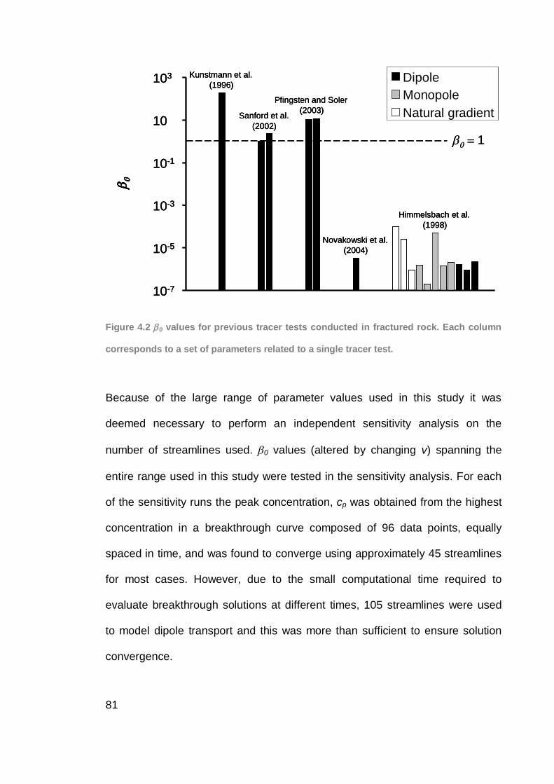
81

Novakowski et al. (2004)

Himmelsbach et al. (1998)

Pfingsten and Soler(2003)Sanford et al.

(2002)

Kunstmann et al. (1996)

10-7

10-5

10-3

10-1

10

103 DipoleMonopoleNatural gradient

1




(2002)


10-7

10-5

10-3

10-1

10





(2002)


10-7

10-5

10-3

10-1

10


1

Figure 4.2 0 values for previous tracer tests conducted in fractured rock. Each column

corresponds to a set of parameters related to a single tracer test.

Because of the large range of parameter values used in this study it was

deemed necessary to perform an independent sensitivity analysis on the

number of streamlines used. 0 values (altered by changing v) spanning the

entire range used in this study were tested in the sensitivity analysis. For each

of the sensitivity runs the peak concentration, cp was obtained from the highest

concentration in a breakthrough curve composed of 96 data points, equally

spaced in time, and was found to converge using approximately 45 streamlines

for most cases. However, due to the small computational time required to

evaluate breakthrough solutions at different times, 105 streamlines were used

to model dipole transport and this was more than sufficient to ensure solution

convergence.

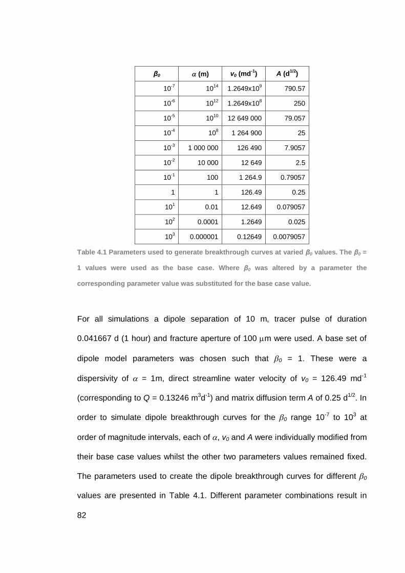
82

0 (m) v0 (md-1) A (d1/2)

10-7 1014 1.2649x109 790.57

10-6 1012 1.2649x108 250

10-5 1010 12 649 000 79.057

10-4 108 1 264 900 25

10-3 1 000 000 126 490 7.9057

10-2 10 000 12 649 2.5

10-1 100 1 264.9 0.79057

1 1 126.49 0.25

101 0.01 12.649 0.079057

102 0.0001 1.2649 0.025

103 0.000001 0.12649 0.0079057

Table 4.1 Parameters used to generate breakthrough curves at varied 0 values. The 0 =

1 values were used as the base case. Where 0 was altered by a parameter the

corresponding parameter value was substituted for the base case value.

For all simulations a dipole separation of 10 m, tracer pulse of duration

0.041667 d (1 hour) and fracture aperture of 100 m were used. A base set of

dipole model parameters was chosen such that 0 = 1. These were a

dispersivity of = 1m, direct streamline water velocity of v0 = 126.49 md-1

(corresponding to Q = 0.13246 m3d-1) and matrix diffusion term A of 0.25 d1/2. In

order to simulate dipole breakthrough curves for the 0 range 10-7 to 103 at

order of magnitude intervals, each of , v0 and A were individually modified from

their base case values whilst the other two parameters values remained fixed.

The parameters used to create the dipole breakthrough curves for different 0

values are presented in Table 4.1. Different parameter combinations result in

83

different time for tracer breakthrough. For each breakthrough curve, 96 data

points equally spaced in time were calculated over durations ranging from 0.1 to

100,000 d. In each case the total time allowed for tracer breakthrough was

chosen such that tracer concentration had peaked and dropped by at least 50

% of the peak concentration.

The generated dipole breakthrough curves were then each fitted by the 1-D flow

model using the parameter estimation program PEST (Doherty, 2004). A range

of initial parameter estimates were used in fitting each of the dipole

breakthrough curves to ensure global best fit parameters were obtained.

Upon completing the fitting process, many initial parameter estimates yielded

poor fits to the dipole breakthrough curves. In order to incorporate only the

successful sets of parameters in the analysis, two fitting criteria were used. One

was the r-squared value, or square of the Pearson product moment correlation

coefficient

2

1

2,

1

2,

1,,

2

n

itartari

n

ifitfiti

n

itartarifitfiti

cccc

ccccr (4.5)

and the other the average normalised residual

n

i tarp

tarifiti

ccc

nE

1 ,

,,1 (4.6)

84

where i = integer counter, n = number of data points in the breakthrough curve

(96 in this study), fit indicates a fitted data value, tar represents a target data

value and overscore indicates an average over the data set.

For each fit, r2 and E were evaluated across the 96 data points. A minimum r2 of

98.5% and a maximum average normalised residual of 10% were specified as

an objective and consistent set of criteria for determining a ‘good’ fit. The

parameters deemed to have generated a good fit were then used to calculate

an average and standard deviation for each parameter.

Results

Figure 4.3 shows a breakthrough curve generated with the dipole model using

= 1 m, v0 = 126.49 md-1 (Q = 0.13246 m3d-1) and A = 2.5 d1/2, along with a 1-D

breakthrough curve optimised to fit the dipole data with resulting parameters =

0.1905 m, v = 289.95 md-1 and A = 0.073508 d1/2. If these breakthrough curves

were the result of optimisation to real field data it would be almost impossible to

determine which model and associated parameter estimates best describe the

system in the absence of additional information. It is now useful to explore the

differences between parameter values for similar breakthrough curves

generated with the two models.

Figure 4.4a shows the normalised (i.e. the fitted 1-D parameter value divided by

the dipole parameter value used to generate the initial breakthrough curve) 1-D

dispersivity values for the range of 0 studied. It is worth noting that dipole and

1-D parameters are up to more than 7 orders of magnitude different. For 1D( )

85

0

0.02

0.04

0.06

0.08

0.1

0.12

0.14

0.16

0 0.2 0.4 0.6 0.8 1t (d)

c/c 0

Dipole1-D

Figure 4.3 A dipole breakthrough curve generated with = 1 m, v0 = 126.49 md-1 (Q =

0.13246 m3d-1) and A = 2.5 d1/2, fitted with a 1-D breakthrough curve with parameters =

0.1905 m, v = 289.95 md-1 and A = 0.073508 d1/2.

(i.e. 0 is altered by whilst holding v0 and A constant) 1D is underestimated

for low 0 (high ) and overestimated for high 0 (low ). This is because 1D( )

values do not vary greatly, all falling between 104 and 106 m, compared with the

span of dipole input values ranging from 10-6 to 1014. Regardless of the

value used in the dipole model to create the breakthrough curves, the 1-D

model always requires a high dispersivity to account for the spreading of solute

along multiple streamlines in the dipole model. 1D( ) is only underestimated by

the 1-D model in regions where the value used to create the dipole

breakthrough is so high that breakthrough is relatively insensitive to changes in

dispersivity. This results from not being an exact descriptor of tracer

behaviour. Either doubling A or multiplying by 16 from an initial set of

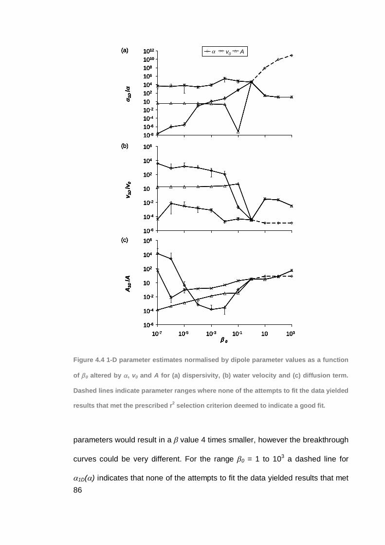
86

10-8

10-6

10-4

10-2

10102

104

106

108

1010

1012

1D/

v0 A(a)

10-8

10-6

10-4

10-2

10102

104

106

108

1010

1012

1D/

v0 A(a)

10-6

10-4

10-2

10

102

104

106

v 1D

/v0

(b)

10-6

10-4

10-2

10

102

104

106

v 1D

/v0

(b)

10-6

10-4

10-2

10

102

104

106

10-7 10-5 10-3 10-1 10 103

0

A1D

/A

(c)

10-6

10-4

10-2

10

102

104

106

10-7 10-5 10-3 10-1 10 103

0

A1D

/A

(c)

10-8

10-6

10-4

10-2

10102

104

106

108

1010

1012

1D/

v0 A(a)

10-8

10-6

10-4

10-2

10102

104

106

108

1010

1012

1D/

v0 A(a)

10-6

10-4

10-2

10

102

104

106

v 1D

/v0

(b)

10-6

10-4

10-2

10

102

104

106

v 1D

/v0

(b)

10-6

10-4

10-2

10

102

104

106

10-7 10-5 10-3 10-1 10 103

0

A1D

/A

(c)

10-6

10-4

10-2

10

102

104

106

10-7 10-5 10-3 10-1 10 103

0

A1D

/A

(c)

Figure 4.4 1-D parameter estimates normalised by dipole parameter values as a function

of 0 altered by , v0 and A for (a) dispersivity, (b) water velocity and (c) diffusion term.

Dashed lines indicate parameter ranges where none of the attempts to fit the data yielded

results that met the prescribed r2 selection criterion deemed to indicate a good fit.

parameters would result in a value 4 times smaller, however the breakthrough

curves could be very different. For the range 0 = 1 to 103 a dashed line for

1D( ) indicates that none of the attempts to fit the data yielded results that met

87

the r2 selection criterion. Results shown are for those runs that met the E

criterion alone. The dipole model, even with no dispersivity applied to individual

streamlines, generates a tailed, smooth breakthrough curve with apparent

dispersion due to the differing arrival times of each of the streamlines. In the

high 0 range, the dipole model has a very low input value. The 1-D model is

no longer able to match the dipole breakthrough simply by reducing the fitted

1D value because, as for the low 0 values, breakthrough is no longer sensitive

to changes in 1D. Hence very similar non-normalised 1D values are returned

for each breakthrough curve. In this same range 1D(v) and 1D(A) are able to

match the dipole breakthrough by reducing the fitted 1D values as

breakthrough for these cases is still sensitive to 1D. It is interesting to note the

remarkable closeness of the normalised 1D(v) and 1D(A) curves from 0 = 1 to

103. In this range, tracer breakthrough is dominated by spreading due to matrix

diffusion. As the influence of dispersion reduces, the transport equation can be

fitted using these two parameters (v and A) alone.

Results for normalised v1D values are presented in Figure 4.4b. As with the

results, dipole breakthrough is relatively insensitive to changes in v for the lower

values of 0 resulting in similar large non-normalised v1D values. Again the

behaviour of v1D(v) and v1D(A) are remarkably alike for 0 = 1 to 103. The 1-D

solution (dashed) was not able to meet the good fit criteria for v1D( ) for the

range 0 = 1 to 103 as previously mentioned.

88

Figure 4.4c shows normalised A1D values. Normalised A1D(A) increases for the

entire 0 range, however the raw (non-normalised) A1D(A) values are

approximately constant for 0 10-2 where diffusion has negligible impact on

breakthrough. This results in a sloped straight line when parameter values are

normalised. A1D( ) and A1D(v) decrease and then increase again as 0

increases. As in the other graphs, normalised A1D(v) and A1D(A) are very

similar.

Normalised 1D values obtained from the composite average parameters are

plotted in Figure 4.5. All three means of altering 0 yield a common trend for

normalised 1D. At low 0, 1D is greater than 0 as diffusion is overestimated.

This overestimation decreases as 0 increases (and scenarios become more

diffusive). This is because at low 0 there is very little diffusion in the direct

streamline of the dipole. However, the long streamlines of the dipole cause the

combined breakthrough to appear as though greater matrix diffusion is

occurring. At higher 0 the dipole model undergoes greater diffusion. The 1D

model interprets the presence of significant diffusion, but the effect of matrix

diffusion is not so overestimated. At high 0 the behaviour caused by modifying

v and A is very similar, as was the case for the three individually tested

parameters.

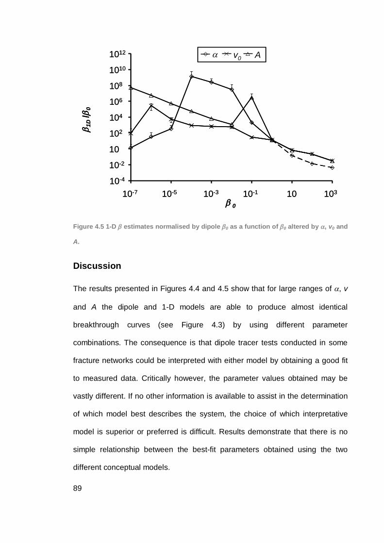
89

10-4

10-2

10

102

104

106

108

1010

1012

10-7 10-5 10-3 10-1 10 103

0

1D/

0

v0 A

10-4

10-2

10

102

104

106

108

1010

1012

10-7 10-5 10-3 10-1 10 103

0

1D/

0

v0 A

Figure 4.5 1-D estimates normalised by dipole 0 as a function of 0 altered by , v0 and

A.

Discussion

The results presented in Figures 4.4 and 4.5 show that for large ranges of , v

and A the dipole and 1-D models are able to produce almost identical

breakthrough curves (see Figure 4.3) by using different parameter

combinations. The consequence is that dipole tracer tests conducted in some

fracture networks could be interpreted with either model by obtaining a good fit

to measured data. Critically however, the parameter values obtained may be

vastly different. If no other information is available to assist in the determination

of which model best describes the system, the choice of which interpretative

model is superior or preferred is difficult. Results demonstrate that there is no

simple relationship between the best-fit parameters obtained using the two

different conceptual models.

90

Possibly more important than the individual parameters obtained from the

interpretation of a tracer test are the predictions of solute transport behaviour

made in a system using these parameters. For example, a dipole tracer test

may be conducted to determine hydraulic and solute transport parameters for

an aquifer in which contamination has occurred, with the aim of ultimately

predicting transport under the natural hydraulic gradient. Weatherill et al. (2006)

showed that when using a single conceptual model, in some cases predictions

of solute transport under lower hydraulic gradients can be better constrained

than individual parameter values. However, if the initial interpretive model

chosen poorly describes the system (even though it may fit the breakthrough

data well), there is potential for large error in subsequent predictions under the

natural hydraulic gradient. As an illustrative example, predictions of transport

from a constant solute source were made for hydraulic gradients of 0.1, 0.01

and 0.001, which for a smooth-walled fracture of aperture 100 m generates

ground water velocities of 61.92, 6.192 and 0.6192 md-1 respectively. The

parameter values from a dipole conceptual model ( = 1 m and A = 2.5 d1/2) and

1-D conceptual model ( = 0.1905 m and A = 0.073508 d1/2) that generated the

breakthrough curves in Figure 4.3 were used. Figure 4.6 shows subsequent

breakthrough 100 m downstream from the solute source using a 1-D transport

solution with these different parameter values. Lower hydraulic gradients (with

greatest difference from the forced gradient conditions) yield larger

discrepancies between the two models, with the time for tracer arrival differing

by up to three orders of magnitude. Thus, a good fit to measured data in a

forced gradient tracer test used for parameter estimation may lead to poor

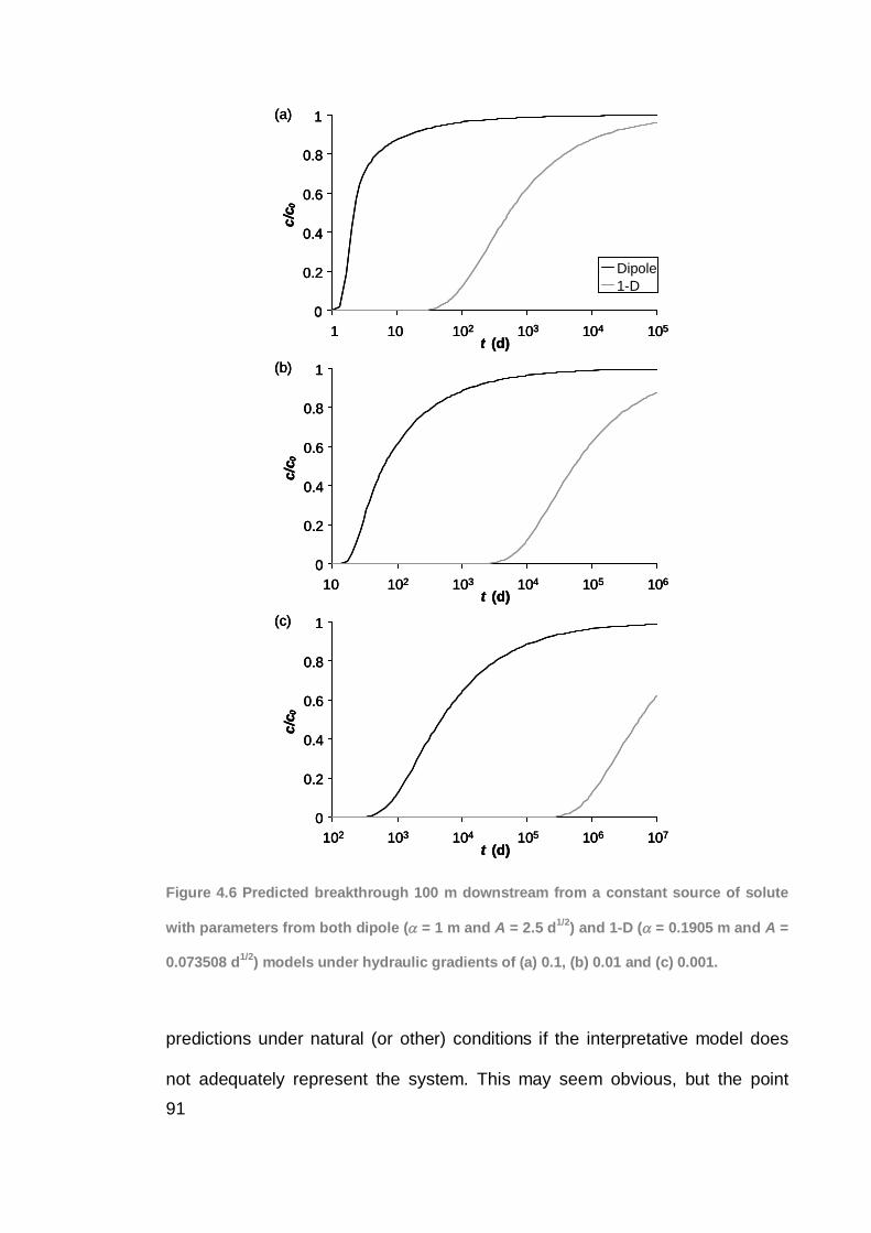
91

0

0.2

0.4

0.6

0.8

1

10 102 103 104 105 106t (d)

c/c 0

(b)

0

0.2

0.4

0.6

0.8

1

102 103 104 105 106 107t (d)

c/c 0

(c)

0

0.2

0.4

0.6

0.8

1

1 10 102 103 104 105t (d)

c/c 0

Dipole1-D

(a)

0

0.2

0.4

0.6

0.8

1

10 102 103 104 105 106t (d)

c/c 0

(b)

0

0.2

0.4

0.6

0.8

1

10 102 103 104 105 106t (d)

c/c 0

(b)

0

0.2

0.4

0.6

0.8

1

102 103 104 105 106 107t (d)

c/c 0

(c)

0

0.2

0.4

0.6

0.8

1

102 103 104 105 106 107t (d)

c/c 0

(c)

0

0.2

0.4

0.6

0.8

1

1 10 102 103 104 105t (d)

c/c 0

Dipole1-D

(a)

0

0.2

0.4

0.6

0.8

1

1 10 102 103 104 105t (d)

c/c 0

Dipole1-D

(a)

Figure 4.6 Predicted breakthrough 100 m downstream from a constant source of solute

with parameters from both dipole ( = 1 m and A = 2.5 d1/2) and 1-D ( = 0.1905 m and A =

0.073508 d1/2) models under hydraulic gradients of (a) 0.1, (b) 0.01 and (c) 0.001.

predictions under natural (or other) conditions if the interpretative model does

not adequately represent the system. This may seem obvious, but the point

92

regarding conceptual model choice is rarely demonstrated explicitly and

quantitatively in ground water hydrology, although the philosophical principle is

well understood.

Given the potentially large errors that can arise from a poor model choice (even

if the model generates a good fit the measured data) any additional information

about the system would assist both in further constraining parameters and

determining which conceptual model may be more appropriate in the

interpretation of field based observations. For this reason multiple tracers with

different aqueous diffusion coefficients are often used in fractured rock tracer

tests with the aim of isolating the effects of dispersion and diffusion on the

resultant breakthrough curves. Similarly tests conducted under different forced

gradients and over different well separations may be useful. Clearly, additional

information on fracture geometry (e.g. orientations, spatial extent and

connectedness) will also be beneficial.

Conclusions

This study has demonstrated the non-uniqueness that arises in the

interpretation of dipole tracer tests conducted in fractured rock, when the

appropriate interpretive model is not known. Breakthrough curves were

generated for a wide range of parameter values using a dipole flow model and

then fitted with a 1-D flow model. The parameter values required for each model

to generate matching breakthrough curves were compared and found to be

vastly (up to more than 7 orders of magnitude) different in many cases, having

important implications for subsequent predictions based on these initial

93

parameter estimations. It is understood that conceptual model choice is a major

issue in hydrogeology, but there are limited quantitative analyses that explicitly

demonstrate the consequences of choosing different conceptual models over

and above the general philosophical principle that it is a vital part of interpreting

field data and making hydrologic predictions.

The key findings of this study are:

5. Dipole tracer test breakthrough curves can be easily fitted with different

conceptual models yielding vastly different estimated parameter values.

Given the similarity of the breakthrough curves it is quite surprising just how

different the parameter values ( , v and A) can be. This is not necessarily

intuitive. The potential impact of the choice of conceptual model can not be

overstated. This reinforces that fact that a good model fit does not

necessarily indicate a unique or correct interpretation of field based data.

6. Use of an incorrect interpretive model to determine aquifer parameters from

a measured breakthrough curve can lead to very large errors in subsequent

predictions (e.g. natural gradient solute transport), even if the fit to the

original forced gradient breakthrough curve is excellent.

7. Additional information (such as the use of multiple tracers, multiple tests

under different forcing conditions or prior knowledge of the extent and

geometry of fractures) that can be used to identify the physical processes

causing the spreading of tracer will assist in the interpretation of dipole

tracer tests conducted in fractured rock.

94

8. For a more complex fractured rock setting, neither of the 1-D or dipole flow

models assessed in this study is a ‘perfect’ representation of a real field

scenario. Further work is required to elucidate where one is a better

approximation than the other. What remains, however, is the potential

disparity between the often simpler interpretative model chosen and the

more complex processes occurring in the real world. This study has

demonstrated differences between the 1-D and dipole interpretative

parameters for a highly simplified and idealised test case. When interpreting

transport in a more complex system, it is likely that both may be a poor

conceptual model choice compared with the real system (which is rarely

known). Further quantifying the disparity between a ‘real’ conceptual model

and simplified interpretative models (e.g. 1-D or dipole) remains a subject for

future inquiry.

95

Notation and Units

Subscript denotes a property of a streamline of departure angle .








E average normalised error -

Q fluid injection/extraction rate L3T-1



r2 square of Pearson product moment

correlation coefficient -

t time T


x, z spatial coordinates L


ratio of diffusive to dispersive time scales -

matrix porosity -


tortuosity -

streamline departure angle rad

96

References

Akin, S., 2005. Tracer model identification using artificial neural networks. Water

Resources Research, 41: W10421, doi:10.1029/2004WR003838.

Becker, M.W. and Shapiro, A.M., 2000. Tracer transport in fractured crystalline

rock: evidence of nondiffusive breakthrough tailing. Water Resources Research,

36(7): 1677-1686.



Grisak, G.E. and Pickens, J.F., 1981. An analytical solution for solute transport

through fractured media with matrix diffusion. Journal of Hydrology, 52: 47-57.

Grove, D.B. and Beetem, W.A., 1971. Porosity and dispersion constant

calculations for a fractured carbonate aquifer using the two well tracer method.

Water Resources Research, 7(1): 128-134.

Himmelsbach, T., Hotzl, H. and Maloszewski, P., 1998. Solute transport

processes in a highly permeable fault zone of Lindau fractured rock test site

(Germany). Ground Water, 36(5): 792-800.

Himmelsbach, T. and Maloszewski, P., 1992. Tracer tests and hydraulic

investigations in the observation tunnel Lindau. Steirische Beitraege zur

Hydrogeologie: 197-228.

Jardine, P.M. et al., 1999. Quantifying diffusive mass transfer in fractured shale

bedrock. Water Resources Research, 35(7): 2015-2030.

Lever, D.A. and Bradbury, M.H., 1985. Rock-matrix diffusion and its implications

for radionuclide migration. Mineralogical Magazine, 49(351): 245-254.

97

Maloszewski, P., Harum, T. and Benischke, R., 1992. Mathematical modelling

of tracer experiments in the karst of Lurbach system, in Application of tracer

models. Steirische Beitraege zur Hydrogeologie: 116-158.

Maloszewski, P., Herrmann, A. and Zuber, A., 1999. Interpretation of tracer

tests performed in fractured rock of the Lange Bramke basin, Germany.

Hydrogeology Journal, 7(2): 209-218.

Neretnieks, I., 1983. A note on fracture flow dispersion mechanisms in the

ground. Water Resources Research, 19(2): 364-370.

Novakowski, K.S., 1988. Comparison of fracture aperture widths determined

from hydraulic measurements and tracer experiments. In: B. Hitchon and S.

Bachu (Editors), Proceedings: 4th Canadian/American Conference on

Hydrogeology. National Water Well Association, Dublin, Ohio, pp. 68-80.

Novakowski, K.S., Bickerton, G. and Lapcevic, P., 2004. Interpretation of

injection-withdrawal tracer experiments conducted between two wells in a large

single fracture. Journal of Contaminant Hydrology, 73: 227-247.




Pfingsten, W. and Soler, J.M., 2003. Modelling of nonreactive tracer dipole tests

in a shear zone at the Grimsel test site. Journal of Contaminant Hydrology, 61:

387-403.



Transactions on Mathematical Software, 10(3): 348-353.

98

Rasmuson, A. and Neretnieks, I., 1986. Radionuclide transport in fast channels

in crystalline rock. Water Resources Research, 22(8): 1247-1256.



Adelaide.



Sudicky, E.A. and Frind, E.O., 1982. Contaminant transport in fractured porous

media: analytical solutions for a system of parallel fractures. Water Resources

Research, 18(6): 1634-1642.




Tsang, C.F., Tsang, Y.W. and Hale, F.V., 1991. Tracer transport in fractures:

analysis of field data based on a variable-aperture channel model. Water


Tsang, Y.W. and Tsang, C.F., 1987. Channel model of flow through fractured

media. Water Resources Research, 23(3): 467-479.

Weatherill, D., Cook, P.G., Simmons, C.T. and Robinson, N.I., 2006. Applied

tracer tests in fractured rock: Can we predict natural gradient solute transport

more accurately than fracture and matrix parameters? Journal of Contaminant

Hydrology, 88: 289-305.

Webster, D.S., Proctor, J.F. and Marine, I.W., 1970. Two-well tracer test in

fractured crystalline rock. US Geological Survey Water Supply Paper, 1544-I.

99

Chapter 5: Interpreting dipole tracer tests in fractured

rock aquifers

Abstract

Dipole tracer tests, where transport of applied tracer is measured in a steady

state injection-withdrawal dipole, provide a means to characterise in-situ solute

transport parameters for fractured rock aquifers. Single fracture analytical

models have been used in previous studies to analyse tracer tests conducted in

single isolated fractures (Novakowski, 1988; Novakowski et al., 2004;

Novakowski et al., 1985) and fracture networks (Himmelsbach et al., 1998;

Himmelsbach and Maloszewski, 1992; Sanford et al., 2002). For tests

conducted in a fracture network it is usually assumed that equivalent single

fracture and matrix parameters can be used to represent the whole network.

This study examines the performance of two single fracture analytical models

when used to interpret simulated tracer tests conducted in hypothetical three-

dimensional fracture networks and dipole tracer tests conducted in the Clare

Valley, South Australia, both in terms of parameter estimation and subsequent

solute transport predictions. The benefit of additional measured tracer data,

either for a tracer with a different diffusion coefficient or for another test at a

different injection and extraction rate is examined. The single fracture models

could be calibrated to generate a good fit to a measured data set, but were not

able to accurately predict solute transport under lower hydraulic gradients for

the networks and field scenarios examined in this study. Simulations of

transport in hypothetical fracture networks indicated that predictions could be

100

most improved by conducting an additional test at a lower injection and

extraction rate.

Introduction

Dipole tracer tests have been used for decades to measure solute transport

through in-situ aquifer material. A dipole tracer test uses an injection-extraction

well pair to generate a steady state hydraulic dipole flow field in the aquifer. A

tracer is introduced at the extraction well and the tracer breakthrough is

measured at the extraction well. A dipole flow field allows sampling of a large

volume of aquifer which can be controlled by the spacing of the wells. The

forced gradient imposed by the dipole flow field enables rapid measurement of

tracer transport. The measured tracer breakthrough curve is used to infer

aquifer properties, usually using an analytical model. Single fracture analytical

models have been used in previous studies to analyse tracer tests conducted in

single isolated fractures (Novakowski, 1988; Novakowski et al., 2004;

Novakowski et al., 1985) and fracture networks (Himmelsbach et al., 1998;

Himmelsbach and Maloszewski, 1992; Sanford et al., 2002). For tests

conducted in a fracture network it is usually assumed implicitly that equivalent

single fracture and matrix parameters can be used to represent the whole

network. The extent to which the complex geometry of a fracture network

affects the interpretation of a dipole tracer test is not known.

Grove and Beetem (1971) outlined a method for modelling a 2-D dipole of equal

pole strength (as would occur in a fracture of infinite extent with smooth parallel

walls). The approach is a summation of breakthrough curves from multiple

101

streamlines. Each streamline has a path length and average flow velocity

dependent on the angle of departure from the injection well. This method has

been widely used to interpret dipole tracer tests conducted in single fractures

(Novakowski, 1988; Novakowski et al., 2004; Novakowski et al., 1985) and in

fracture networks (Himmelsbach et al., 1998; Himmelsbach and Maloszewski,

1992; Sanford et al., 2002; Webster et al., 1970).

Typically dipole tracer tests are analysed assuming that a perfect dipole is

attained in the fracture(s). However, laterally finite fractures and variable

fracture apertures channel flow such that infinite dipole flow fields cannot

develop. In some cases a 1-D flow model may in fact better describe the flow

field generated by an injection-extraction well pair. 1-D flow models have also

previously been used to interpret dipole tracer tests where injection and

extraction rates are not equal (Pfingsten and Soler, 2003). Thus a range of

possible interpretative models exist and are subjectively applied. Systematic

evaluation of their behaviour is warranted.

The first part of this study examines the performance of the two single fracture

analytical models (1-D and dipole flow) when used to interpret simulated dipole

tracer tests conducted in hypothetical three-dimensional fracture networks. The

results are demonstrative only and the synthetic fracture networks are not

moderated using real field data. Initially a single dipole tracer test is simulated

numerically in a hypothetical fracture network. The analytical models are

calibrated to the modelled tracer breakthrough curve and used to predict solute

transport under a much lower hydraulic gradient. The predicted solute transport

102

is then compared to the ‘real’ simulated transport. In this way the consequences

of the single fracture approximation and associated flow geometry of the two

interpretative analytical models are identified. The study then examines how the

predictive capability of the analytical models might be improved if additional

information was available to calibrate them. The value of the following is

examined: (a) an extra tracer test at either higher or lower hydraulic gradient,

(b) an additional tracer with a different diffusion coefficient included in the initial

tracer test and (c) knowledge of the length of the shortest fracture flow path

between the injection and extraction wells (rather than an assumption of a

straight line).

The second section of this study applies the methodology used in the

hypothetical fracture networks to real dipole tracer tests conducted in the Clare

Valley, South Australia. Application of the methodology to the field environment

introduces additional variations between the assumptions of the analytical

models and the reality of the field setting.

Generating Synthetic Fracture Networks

For this study three fracture networks were created, each consisting of ten

orthogonal fractures in the x-y and y-z planes. The use of three networks was

deemed sufficient to meet the demonstrative aim of this study. By generating

fractures in two orthogonal orientations, tracer transport could be simulated in a

three-dimensional network of interconnected fractures, rather than simply in

parallel fractures that do not interact directly. Fracture apertures were chosen

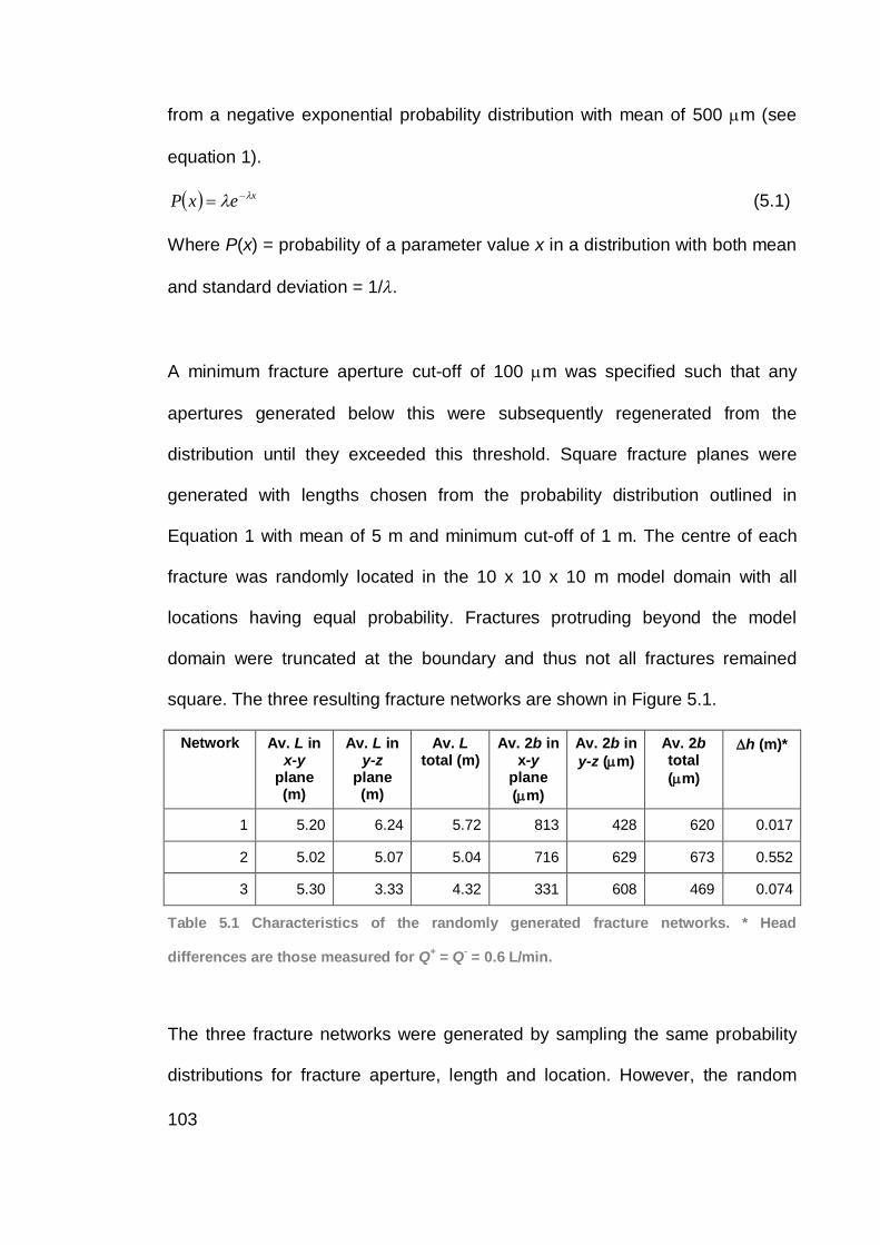
103

from a negative exponential probability distribution with mean of 500 m (see

equation 1).

xexP (5.1)

Where P(x) = probability of a parameter value x in a distribution with both mean

and standard deviation = 1/ .

A minimum fracture aperture cut-off of 100 m was specified such that any

apertures generated below this were subsequently regenerated from the

distribution until they exceeded this threshold. Square fracture planes were

generated with lengths chosen from the probability distribution outlined in

Equation 1 with mean of 5 m and minimum cut-off of 1 m. The centre of each

fracture was randomly located in the 10 x 10 x 10 m model domain with all

locations having equal probability. Fractures protruding beyond the model

domain were truncated at the boundary and thus not all fractures remained

square. The three resulting fracture networks are shown in Figure 5.1.

Network Av. L in x-y

plane (m)

Av. L in y-z

plane (m)

Av. L total (m)

Av. 2b in x-y

plane ( m)

Av. 2b in y-z ( m)

Av. 2b total ( m)

h (m)*

1 5.20 6.24 5.72 813 428 620 0.017

2 5.02 5.07 5.04 716 629 673 0.552

3 5.30 3.33 4.32 331 608 469 0.074

Table 5.1 Characteristics of the randomly generated fracture networks. * Head

differences are those measured for Q+ = Q- = 0.6 L/min.

The three fracture networks were generated by sampling the same probability

distributions for fracture aperture, length and location. However, the random

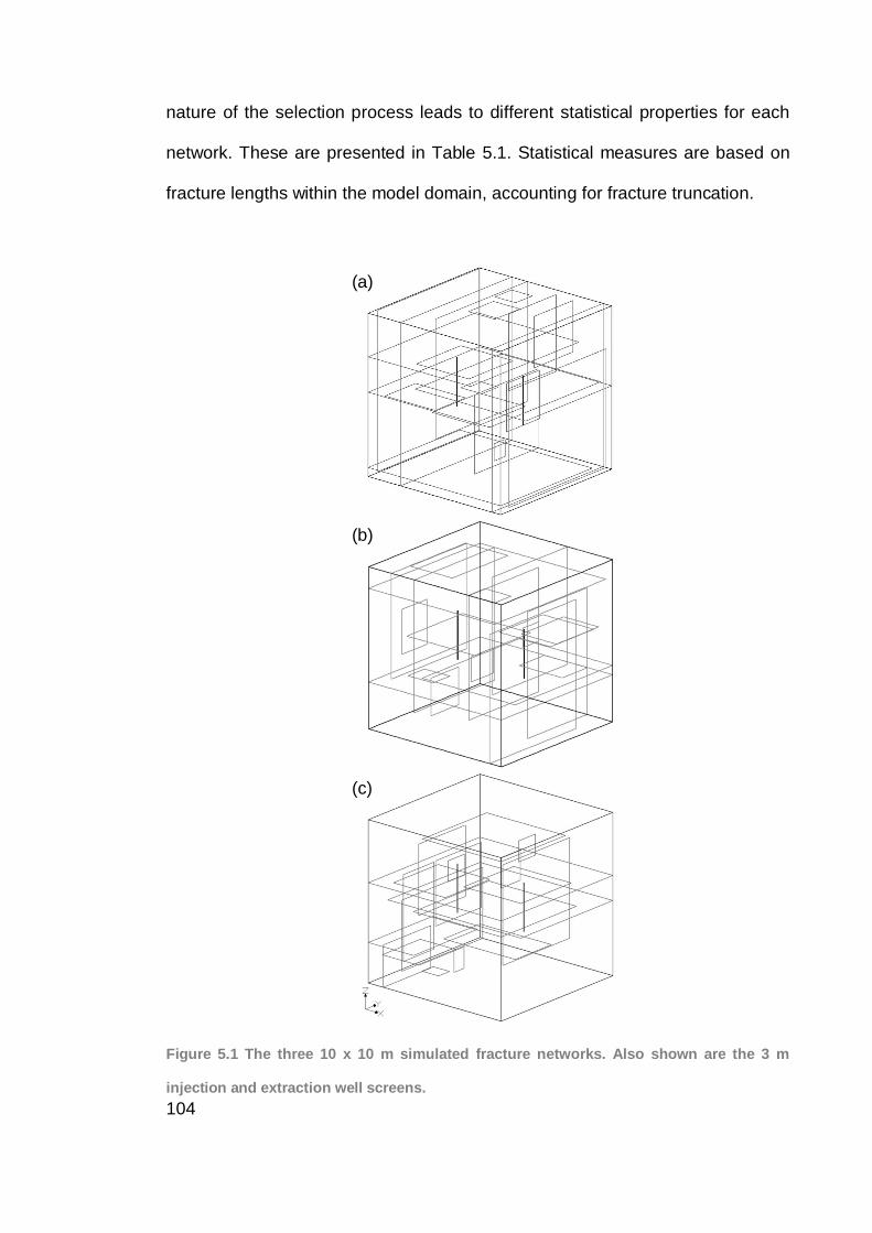
104

nature of the selection process leads to different statistical properties for each

network. These are presented in Table 5.1. Statistical measures are based on

fracture lengths within the model domain, accounting for fracture truncation.

(a)

(b)

(c)

Figure 5.1 The three 10 x 10 m simulated fracture networks. Also shown are the 3 m

injection and extraction well screens.

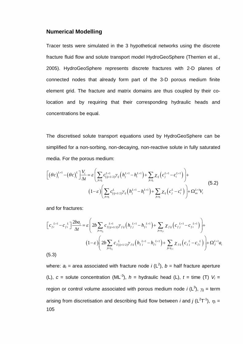
105

Numerical Modelling

Tracer tests were simulated in the 3 hypothetical networks using the discrete

fracture fluid flow and solute transport model HydroGeoSphere (Therrien et al.,

2005). HydroGeoSphere represents discrete fractures with 2-D planes of

connected nodes that already form part of the 3-D porous medium finite

element grid. The fracture and matrix domains are thus coupled by their co-

location and by requiring that their corresponding hydraulic heads and

concentrations be equal.

The discretised solute transport equations used by HydroGeoSphere can be

simplified for a non-sorbing, non-decaying, non-reactive solute in fully saturated

media. For the porous medium:

1 1 1 1 1 11/ 2

1 1 11/ 21

i i

i i

L L L L L L Liij j i ij j iiji i

j j

L L L L L Lij j i ij j i ex iij

j j

Vc c c h h c ct

c h h c c V

(5.2)

and for fractures:

1 1 1 1 1 11/ 2

1 1 11/ 2

2 2

1 2

f f ii

f f ii

L L L L L L Lif i f i f f ij f j f i f ij f j f iij

j j

L L L L L Lf f ij f j f i f ij f j f i f iij

j j

bac c b c h h c ct

b c h h c c a

(5.3)

where: ai = area associated with fracture node i (L2), b = half fracture aperture

(L), c = solute concentration (ML-3), h = hydraulic head (L), t = time (T) Vi =

region or control volume associated with porous medium node i (L3), ij = term

arising from discretisation and describing fluid flow between i and j (L2T-1), i =

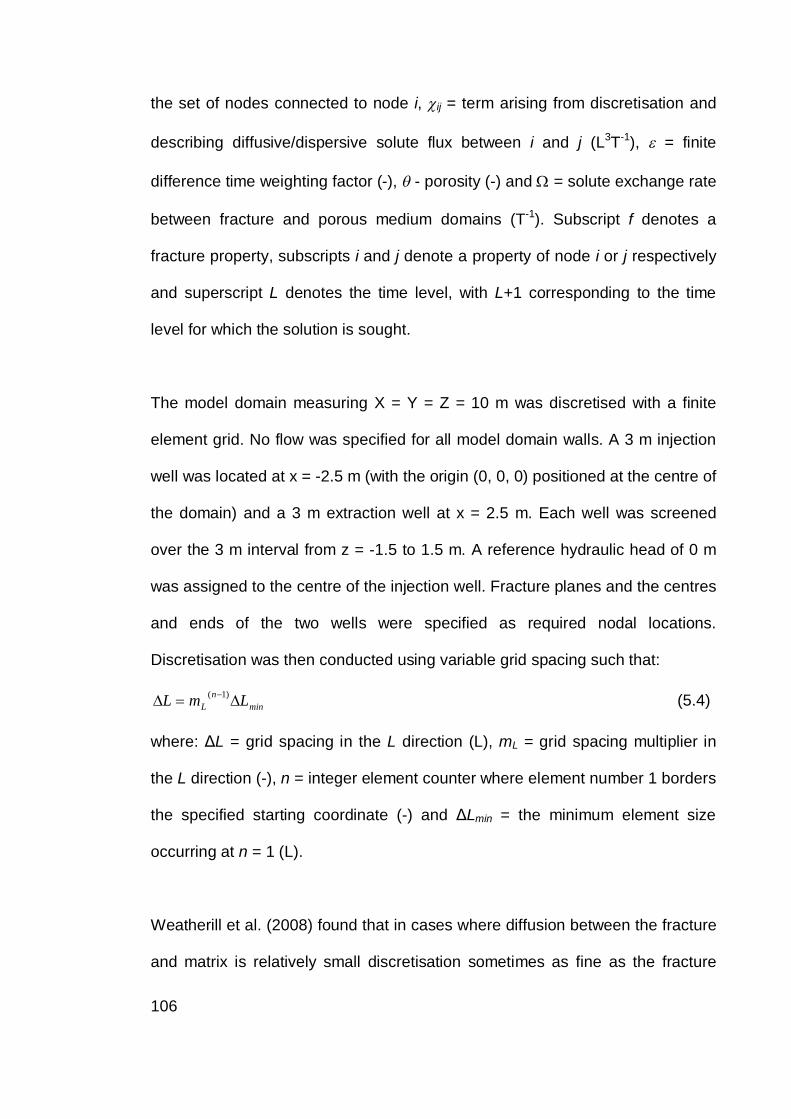
106

the set of nodes connected to node i, ij = term arising from discretisation and

describing diffusive/dispersive solute flux between i and j (L3T-1), = finite

difference time weighting factor (-), - porosity (-) and = solute exchange rate

between fracture and porous medium domains (T-1). Subscript f denotes a

fracture property, subscripts i and j denote a property of node i or j respectively

and superscript L denotes the time level, with L+1 corresponding to the time

level for which the solution is sought.

The model domain measuring X = Y = Z = 10 m was discretised with a finite

element grid. No flow was specified for all model domain walls. A 3 m injection

well was located at x = -2.5 m (with the origin (0, 0, 0) positioned at the centre of

the domain) and a 3 m extraction well at x = 2.5 m. Each well was screened

over the 3 m interval from z = -1.5 to 1.5 m. A reference hydraulic head of 0 m

was assigned to the centre of the injection well. Fracture planes and the centres

and ends of the two wells were specified as required nodal locations.

Discretisation was then conducted using variable grid spacing such that:

minn

L LmL )1( (5.4)

where: L = grid spacing in the L direction (L), mL = grid spacing multiplier in

the L direction (-), n = integer element counter where element number 1 borders

the specified starting coordinate (-) and Lmin = the minimum element size

occurring at n = 1 (L).

Weatherill et al. (2008) found that in cases where diffusion between the fracture

and matrix is relatively small discretisation sometimes as fine as the fracture

107

aperture is required. This study simulates tracer migration under highly forced

conditions where fluid velocities are high and the time available for diffusion into

the matrix is reduced. Hence it was considered prudent to employ fine

discretisation at the fracture-matrix interface. At each fracture plane Lmin was

set to the size of the fracture aperture to ensure a sufficiently fine spatial

discretisation. Following the recommendations of Weatherill et al. (2008) a

sensitivity analysis to mL over the range of forcing conditions was conducted

and a value of 4 was adopted for discretisation moving away from fracture

planes. At the wells Lmin = 0.05 m and mL = 2 were used. A global maximum

grid spacing of 0.5 m was enforced to avoid potential numerical problems

associated with large elements. Because each network employed a different

realisation of fracture locations and apertures, they necessarily employed

different spatial discretisation.

Temporal discretisation was conducted using HydroGeoSphere’s variable time-

stepping procedure with a Crank-Nicolson implicit finite difference scheme in

time, with = 0.5 in equations (2) and (3). Once a solution at time L is found, the

next time-step is determined by:

LL

iL

i

maxL tcc

ct1

1

max (5.5)

where cmax = specified maximum change in concentration desired in a time-step

and ci = calculated concentration at node i. This procedure allows the model to

increase time-step size when there are only small changes in concentration and

reduce it when rapid changes occur. Computation time is reduced without

decreasing numerical accuracy. This study used a very small initial time-step of

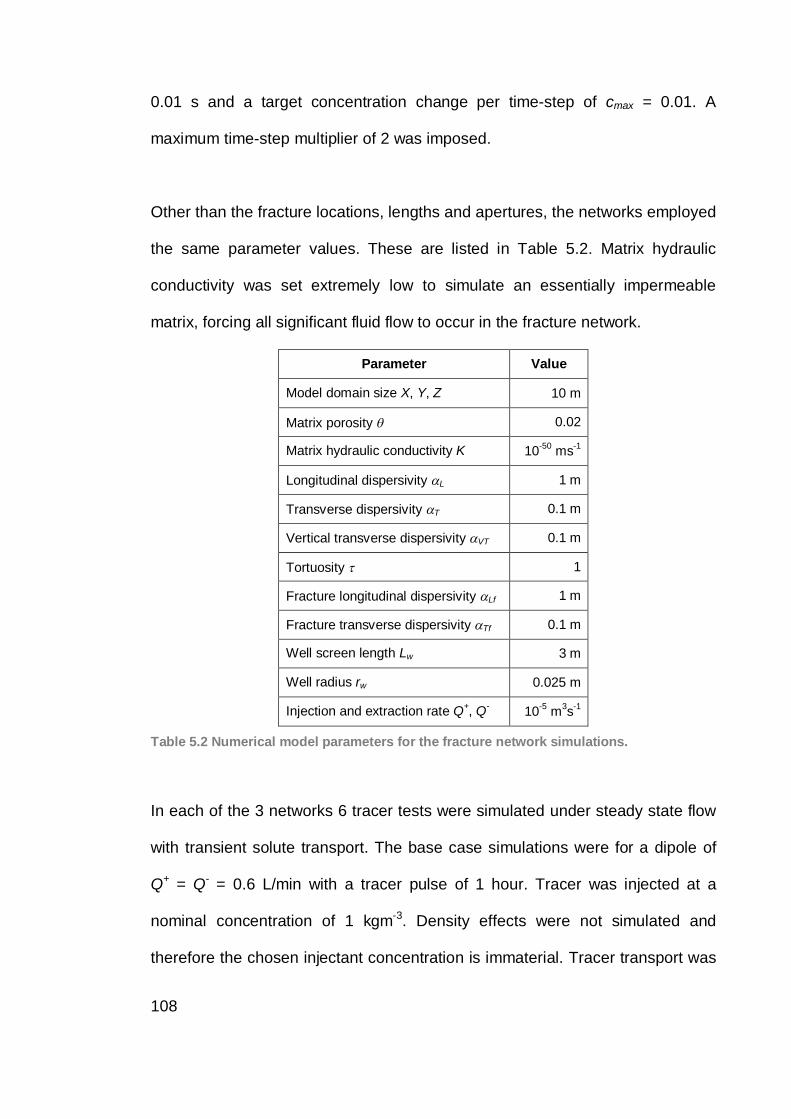
108

0.01 s and a target concentration change per time-step of cmax = 0.01. A

maximum time-step multiplier of 2 was imposed.

Other than the fracture locations, lengths and apertures, the networks employed

the same parameter values. These are listed in Table 5.2. Matrix hydraulic

conductivity was set extremely low to simulate an essentially impermeable

matrix, forcing all significant fluid flow to occur in the fracture network.

Parameter Value

Model domain size X, Y, Z 10 m

Matrix porosity 0.02

Matrix hydraulic conductivity K 10-50 ms-1

Longitudinal dispersivity L 1 m

Transverse dispersivity T 0.1 m

Vertical transverse dispersivity VT 0.1 m

Tortuosity 1

Fracture longitudinal dispersivity Lf 1 m

Fracture transverse dispersivity Tf 0.1 m

Well screen length Lw 3 m

Well radius rw 0.025 m

Injection and extraction rate Q+, Q- 10-5 m3s-1

Table 5.2 Numerical model parameters for the fracture network simulations.

In each of the 3 networks 6 tracer tests were simulated under steady state flow

with transient solute transport. The base case simulations were for a dipole of

Q+ = Q- = 0.6 L/min with a tracer pulse of 1 hour. Tracer was injected at a

nominal concentration of 1 kgm-3. Density effects were not simulated and

therefore the chosen injectant concentration is immaterial. Tracer transport was

109

simulated for 1 day. Additional tracer tests were simulated at factors of 10, 0.1,

0.01, 0.001 and 0.0001 of the base case pumping rates. All simulations were for

1 hour of tracer input, but recovery periods were modified in order to obtain

tracer breakthrough curves which had peaked and begun decreasing. Tracer

aqueous diffusion coefficients of 2.01 x 10-9 m2/s and 1.27 x 10-9 m2/s were

used to simulate bromide (Br-) and sulphur hexafluoride (SF6) respectively.

Initial tracer concentration was set to zero throughout the domain.

Analytical Modelling

The breakthrough curves generated by HydroGeoSphere were fitted using two

single-fracture analytical models, first to obtain interpreted aquifer parameters

and then to make predictions of the other tests. The least-squares parameter

estimation program PEST (Doherty, 2004) was used to fit the analytical models

to the numerical data. Weights were assigned to data values, calculated as 1/cp,

so that when fitting multiple breakthrough curves those with higher

concentrations would not dominate the fitting process. The analytical models

were those for 1-D flow in a single ‘parallel plate’ fracture (Tang et al., 1981)

and one using the approach of Grove and Beetem (1971) to sum breakthrough

curves from multiple streamlines, each representative of a flow line in a 2-D

dipole flow field constrained to the fracture plane. Transport along each

streamline was solved using the Tang et al. (1981) model. Therefore the only

difference between the two analytical models was the flow geometry.

110



repeated here.

The geometry and solution for the model presented by Grove and Beetem

(1971) is outlined in Chapter 4 (see Figure 4.1 and equations 4.1 to 4.3b) and is

not repeated here.

Himmelsbach and Maloszewski (1992) used 120 streamlines to model dipole

tracer breakthrough. Novakowski et al. (1985) found that as few as 12

streamlines were necessary to model unequal strength dipole flow when using a

numerical approach whilst Novakowski et al. (2004) found that 45 streamlines

were needed for convergence using the same numerical technique to model a

dipole with an ambient ground water flow. We conducted an independent

sensitivity analysis and found that approximately 45 streamlines were sufficient

for solution convergence for most parameter combinations. However, due to the

short computational time required, 105 streamlines were used to model dipole

transport and this was more than sufficient to ensure solution convergence.

Initially the analytical models were calibrated using data from the base case (Q+

= Q- = 0.6 L/min) Br- breakthrough curves only. Predicted breakthrough curves

were then generated with both analytical models using the calibrated

parameters, but now with scaled pumping rates and corresponding changes to

v. Now knowing the predictive capabilities of the calibrated models for each of

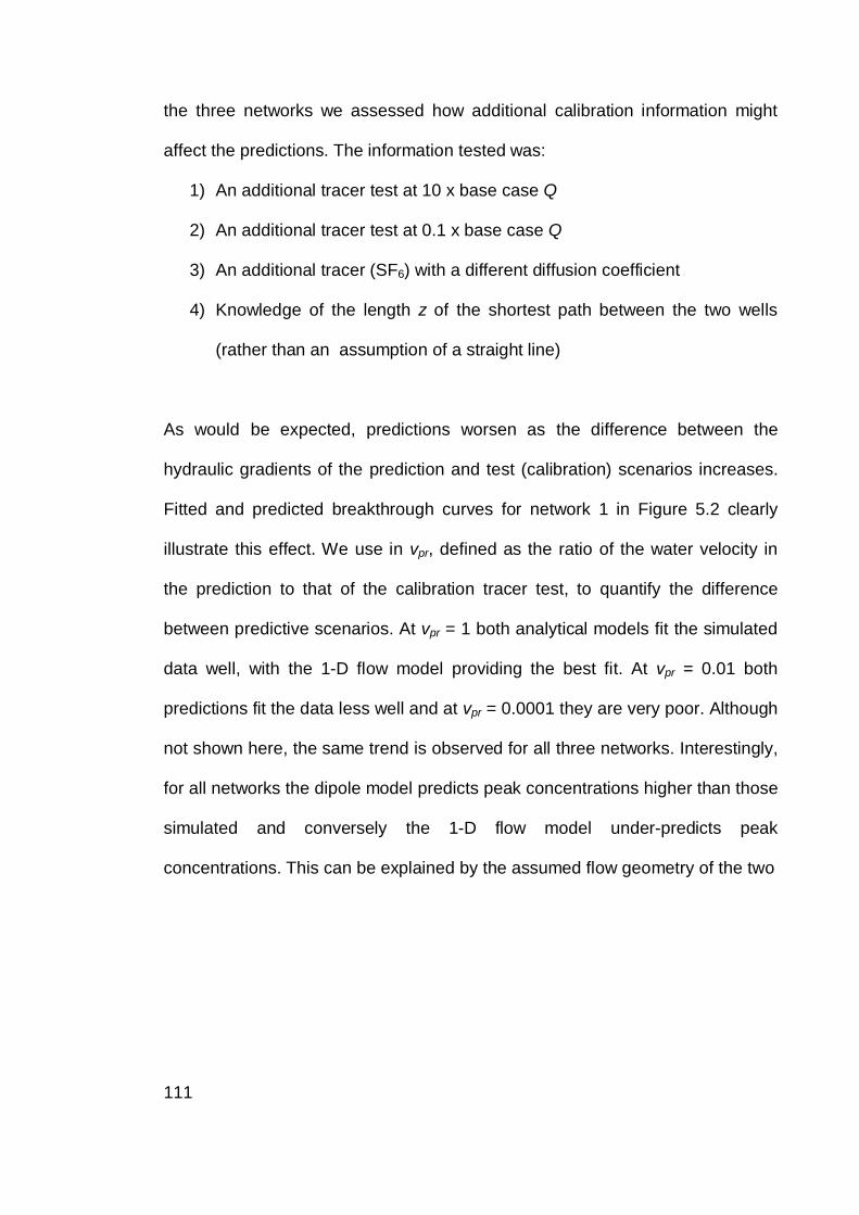
111

the three networks we assessed how additional calibration information might

affect the predictions. The information tested was:

1) An additional tracer test at 10 x base case Q

2) An additional tracer test at 0.1 x base case Q

3) An additional tracer (SF6) with a different diffusion coefficient

4) Knowledge of the length z of the shortest path between the two wells

(rather than an assumption of a straight line)

As would be expected, predictions worsen as the difference between the

hydraulic gradients of the prediction and test (calibration) scenarios increases.

Fitted and predicted breakthrough curves for network 1 in Figure 5.2 clearly

illustrate this effect. We use in vpr, defined as the ratio of the water velocity in

the prediction to that of the calibration tracer test, to quantify the difference

between predictive scenarios. At vpr = 1 both analytical models fit the simulated

data well, with the 1-D flow model providing the best fit. At vpr = 0.01 both

predictions fit the data less well and at vpr = 0.0001 they are very poor. Although

not shown here, the same trend is observed for all three networks. Interestingly,

for all networks the dipole model predicts peak concentrations higher than those

simulated and conversely the 1-D flow model under-predicts peak

concentrations. This can be explained by the assumed flow geometry of the two

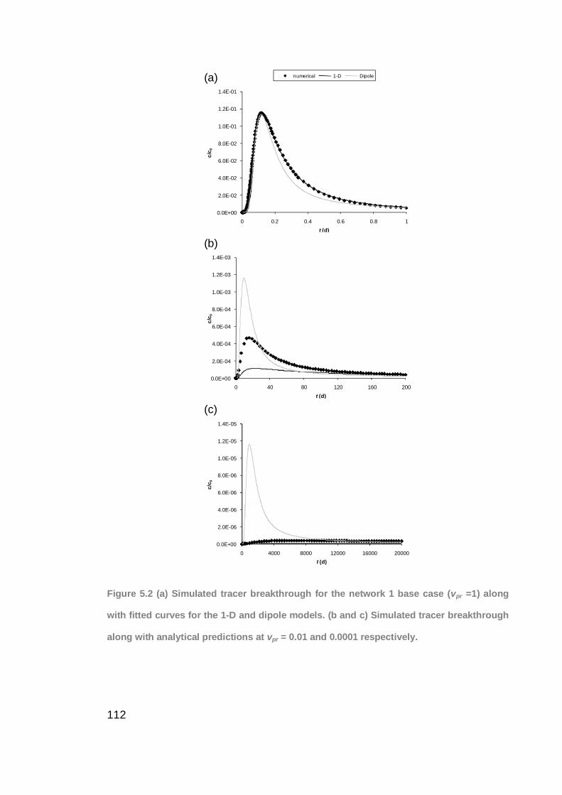
112

0.0E+00

2.0E-02

4.0E-02

6.0E-02

8.0E-02

1.0E-01

1.2E-01

1.4E-01

0 0.2 0.4 0.6 0.8 1

c/c 0

t (d)

numerical 1-D Dipole

0.0E+00

2.0E-04

4.0E-04

6.0E-04

8.0E-04

1.0E-03

1.2E-03

1.4E-03

0 40 80 120 160 200

c/c 0

t (d)

0.0E+00

2.0E-06

4.0E-06

6.0E-06

8.0E-06

1.0E-05

1.2E-05

1.4E-05

0 4000 8000 12000 16000 20000

c/c 0

t (d)

(a)

(b)

(c)

Figure 5.2 (a) Simulated tracer breakthrough for the network 1 base case (vpr =1) along

with fitted curves for the 1-D and dipole models. (b and c) Simulated tracer breakthrough

along with analytical predictions at vpr = 0.01 and 0.0001 respectively.

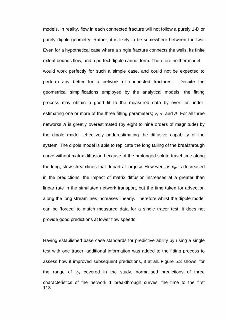
113

models. In reality, flow in each connected fracture will not follow a purely 1-D or

purely dipole geometry. Rather, it is likely to be somewhere between the two.

Even for a hypothetical case where a single fracture connects the wells, its finite

extent bounds flow, and a perfect dipole cannot form. Therefore neither model

would work perfectly for such a simple case, and could not be expected to

perform any better for a network of connected fractures. Despite the

geometrical simplifications employed by the analytical models, the fitting

process may obtain a good fit to the measured data by over- or under-

estimating one or more of the three fitting parameters; v, , and A. For all three

networks A is greatly overestimated (by eight to nine orders of magnitude) by

the dipole model, effectively underestimating the diffusive capability of the

system. The dipole model is able to replicate the long tailing of the breakthrough

curve without matrix diffusion because of the prolonged solute travel time along

the long, slow streamlines that depart at large . However, as vpr is decreased

in the predictions, the impact of matrix diffusion increases at a greater than

linear rate in the simulated network transport, but the time taken for advection

along the long streamlines increases linearly. Therefore whilst the dipole model

can be ‘forced’ to match measured data for a single tracer test, it does not

provide good predictions at lower flow speeds.

Having established base case standards for predictive ability by using a single

test with one tracer, additional information was added to the fitting process to

assess how it improved subsequent predictions, if at all. Figure 5.3 shows, for

the range of vpr covered in the study, normalised predictions of three

characteristics of the network 1 breakthrough curves; the time to the first

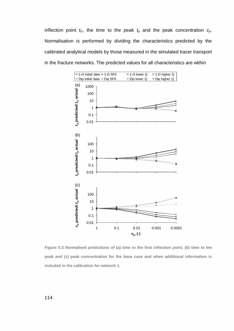
114

inflection point ti1, the time to the peak tp and the peak concentration cp.

Normalisation is performed by dividing the characteristics predicted by the

calibrated analytical models by those measured in the simulated tracer transport

in the fracture networks. The predicted values for all characteristics are within

0.01

0.1

1

10

100

1000

t i1pr

edic

ted/

t i1

actu

al1-D initial data 1-D SF6 1-D lower Q 1-D higher QDip initial data Dip SF6 Dip lower Q Dip higher Q

0.01

0.1

1

10

100

t ppr

edic

ted/

t pac

tual

0.01

0.1

1

10

100

0.00010.0010.010.11c ppr

edic

ted/

cp

actu

al

vpr (-)

(a)

(b)

(c)

Figure 5.3 Normalised predictions of (a) time to the first inflection point, (b) time to the

peak and (c) peak concentration for the base case and when additional information is

included in the calibration for network 1.

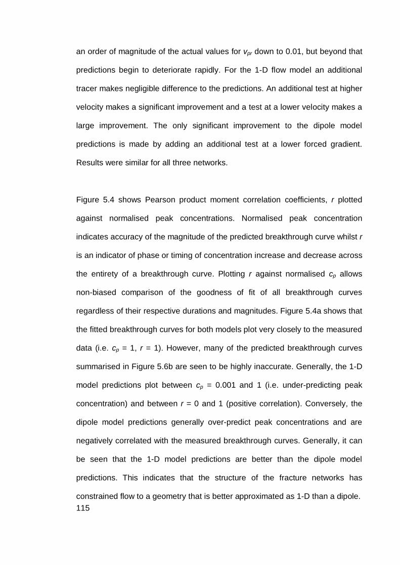
115

an order of magnitude of the actual values for vpr down to 0.01, but beyond that

predictions begin to deteriorate rapidly. For the 1-D flow model an additional

tracer makes negligible difference to the predictions. An additional test at higher

velocity makes a significant improvement and a test at a lower velocity makes a

large improvement. The only significant improvement to the dipole model

predictions is made by adding an additional test at a lower forced gradient.

Results were similar for all three networks.

Figure 5.4 shows Pearson product moment correlation coefficients, r plotted

against normalised peak concentrations. Normalised peak concentration

indicates accuracy of the magnitude of the predicted breakthrough curve whilst r

is an indicator of phase or timing of concentration increase and decrease across

the entirety of a breakthrough curve. Plotting r against normalised cp allows

non-biased comparison of the goodness of fit of all breakthrough curves

regardless of their respective durations and magnitudes. Figure 5.4a shows that

the fitted breakthrough curves for both models plot very closely to the measured

data (i.e. cp = 1, r = 1). However, many of the predicted breakthrough curves

summarised in Figure 5.6b are seen to be highly inaccurate. Generally, the 1-D

model predictions plot between cp = 0.001 and 1 (i.e. under-predicting peak

concentration) and between r = 0 and 1 (positive correlation). Conversely, the

dipole model predictions generally over-predict peak concentrations and are

negatively correlated with the measured breakthrough curves. Generally, it can

be seen that the 1-D model predictions are better than the dipole model

predictions. This indicates that the structure of the fracture networks has

constrained flow to a geometry that is better approximated as 1-D than a dipole.

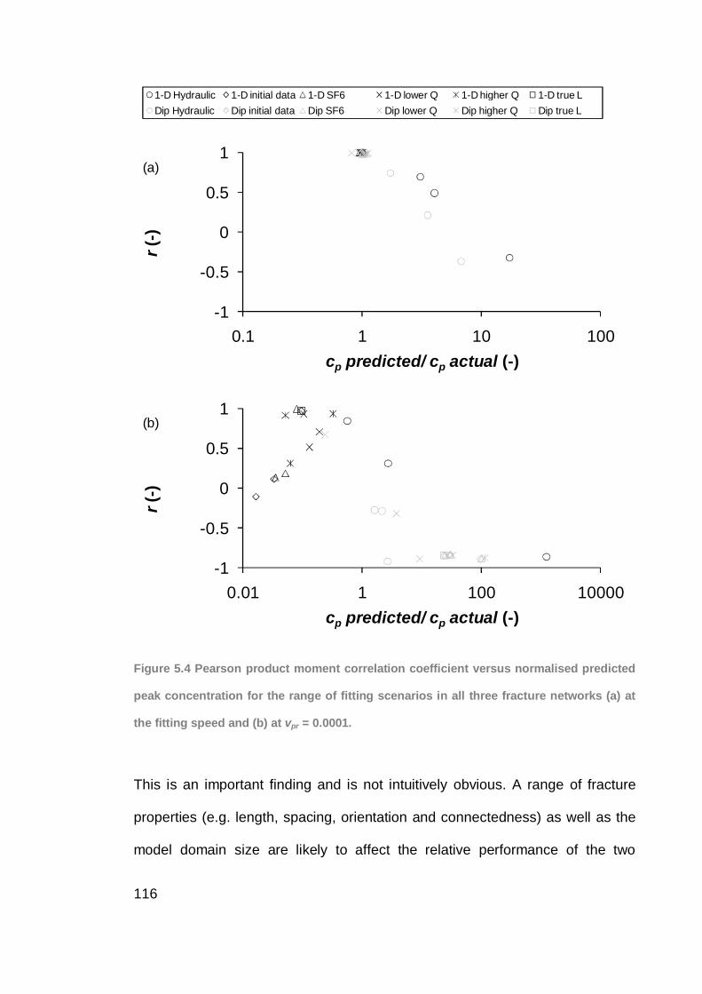
116

-1

-0.5

0

0.5

1

0.1 1 10 100

r(-)

cp predicted/ cp actual (-)

1-D Hydraulic 1-D initial data 1-D SF6 1-D lower Q 1-D higher Q 1-D true LDip Hydraulic Dip initial data Dip SF6 Dip lower Q Dip higher Q Dip true L

-1

-0.5

0

0.5

1

0.01 1 100 10000

r(-)

cp predicted/ cp actual (-)

(a)

(b)

Figure 5.4 Pearson product moment correlation coefficient versus normalised predicted

peak concentration for the range of fitting scenarios in all three fracture networks (a) at

the fitting speed and (b) at vpr = 0.0001.

This is an important finding and is not intuitively obvious. A range of fracture

properties (e.g. length, spacing, orientation and connectedness) as well as the

model domain size are likely to affect the relative performance of the two

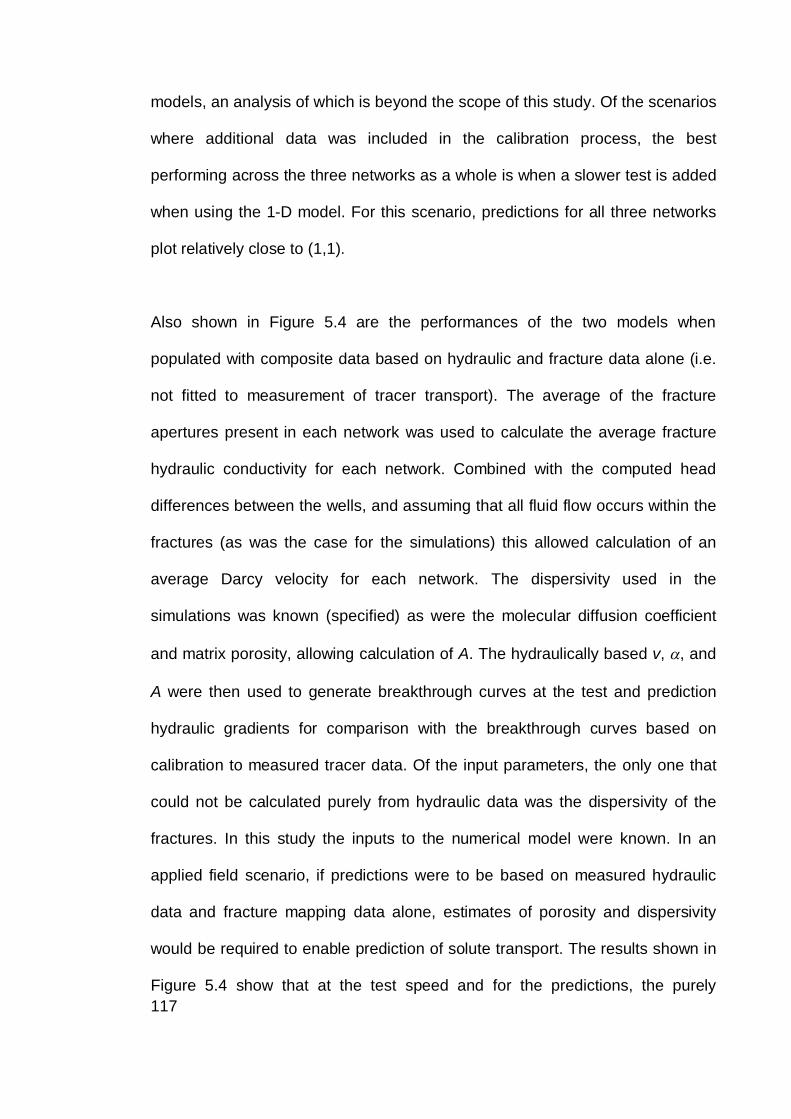
117

models, an analysis of which is beyond the scope of this study. Of the scenarios

where additional data was included in the calibration process, the best

performing across the three networks as a whole is when a slower test is added

when using the 1-D model. For this scenario, predictions for all three networks

plot relatively close to (1,1).

Also shown in Figure 5.4 are the performances of the two models when

populated with composite data based on hydraulic and fracture data alone (i.e.

not fitted to measurement of tracer transport). The average of the fracture

apertures present in each network was used to calculate the average fracture

hydraulic conductivity for each network. Combined with the computed head

differences between the wells, and assuming that all fluid flow occurs within the

fractures (as was the case for the simulations) this allowed calculation of an

average Darcy velocity for each network. The dispersivity used in the

simulations was known (specified) as were the molecular diffusion coefficient

and matrix porosity, allowing calculation of A. The hydraulically based v, , and

A were then used to generate breakthrough curves at the test and prediction

hydraulic gradients for comparison with the breakthrough curves based on

calibration to measured tracer data. Of the input parameters, the only one that

could not be calculated purely from hydraulic data was the dispersivity of the

fractures. In this study the inputs to the numerical model were known. In an

applied field scenario, if predictions were to be based on measured hydraulic

data and fracture mapping data alone, estimates of porosity and dispersivity

would be required to enable prediction of solute transport. The results shown in

Figure 5.4 show that at the test speed and for the predictions, the purely

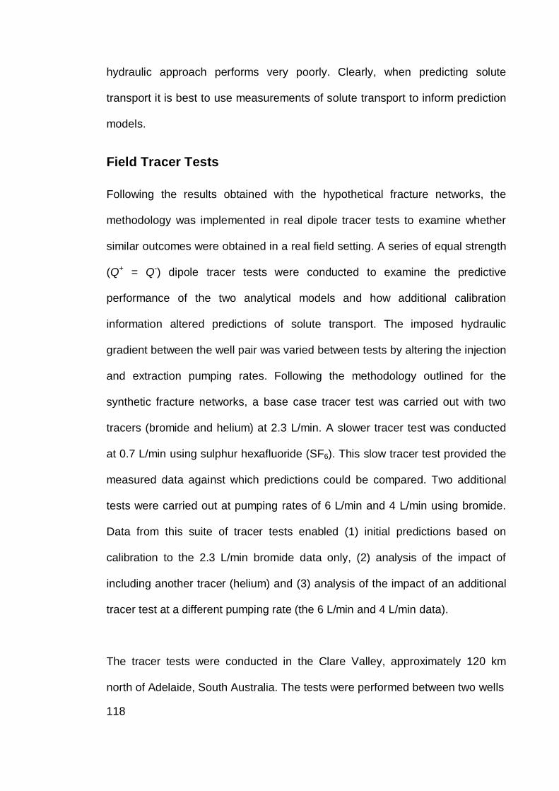
118

hydraulic approach performs very poorly. Clearly, when predicting solute

transport it is best to use measurements of solute transport to inform prediction

models.

Field Tracer Tests

Following the results obtained with the hypothetical fracture networks, the

methodology was implemented in real dipole tracer tests to examine whether

similar outcomes were obtained in a real field setting. A series of equal strength

(Q+ = Q-) dipole tracer tests were conducted to examine the predictive

performance of the two analytical models and how additional calibration

information altered predictions of solute transport. The imposed hydraulic

gradient between the well pair was varied between tests by altering the injection

and extraction pumping rates. Following the methodology outlined for the

synthetic fracture networks, a base case tracer test was carried out with two

tracers (bromide and helium) at 2.3 L/min. A slower tracer test was conducted

at 0.7 L/min using sulphur hexafluoride (SF6). This slow tracer test provided the

measured data against which predictions could be compared. Two additional

tests were carried out at pumping rates of 6 L/min and 4 L/min using bromide.

Data from this suite of tracer tests enabled (1) initial predictions based on

calibration to the 2.3 L/min bromide data only, (2) analysis of the impact of

including another tracer (helium) and (3) analysis of the impact of an additional

tracer test at a different pumping rate (the 6 L/min and 4 L/min data).

The tracer tests were conducted in the Clare Valley, approximately 120 km

north of Adelaide, South Australia. The tests were performed between two wells

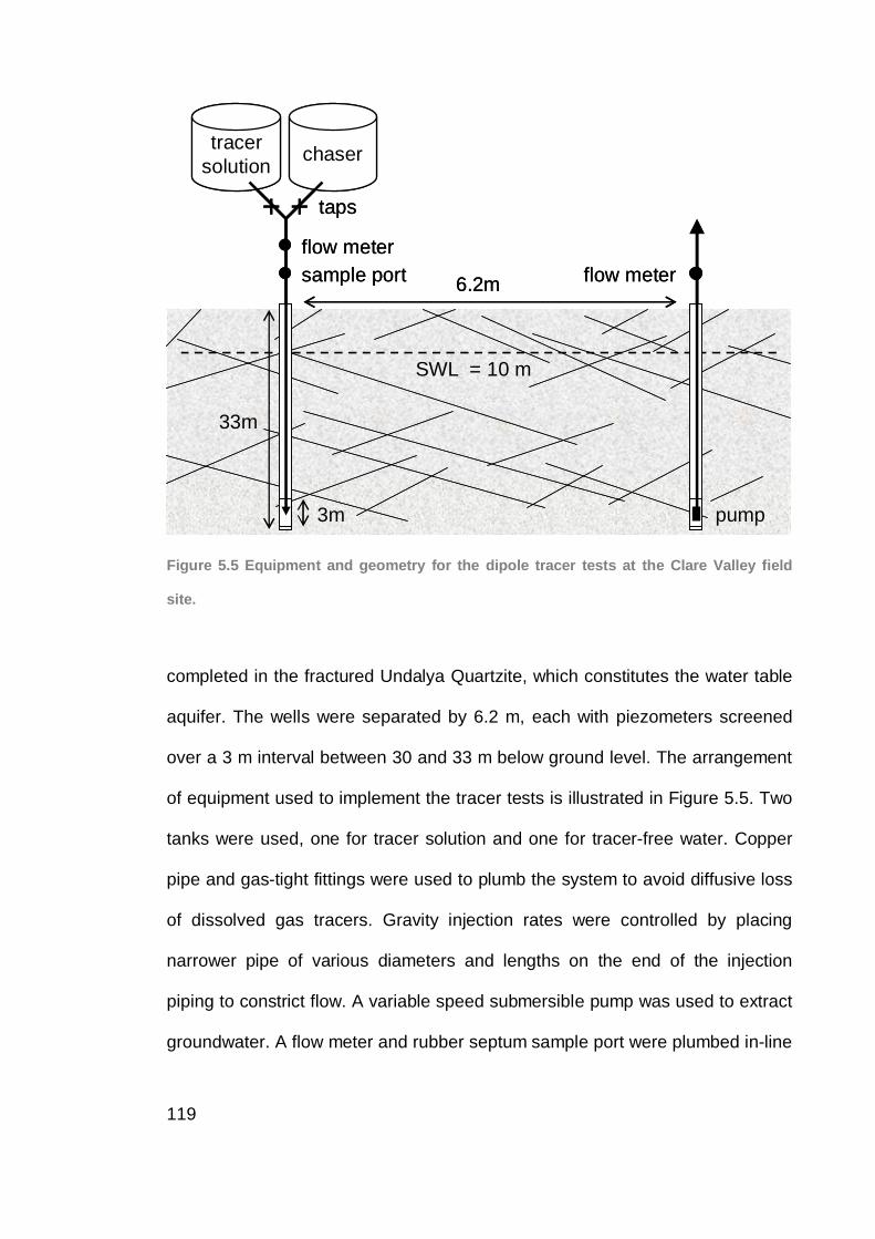
119

tracersolution chaser

+

sample port

taps

pump

flow meterflow meter6.2m

3m

33m

SWL = 10 m

+

tracersolution chaser

+

sample port

taps

pump

flow meterflow meter6.2m

3m

33m

SWL = 10 m

+

Figure 5.5 Equipment and geometry for the dipole tracer tests at the Clare Valley field

site.

completed in the fractured Undalya Quartzite, which constitutes the water table

aquifer. The wells were separated by 6.2 m, each with piezometers screened

over a 3 m interval between 30 and 33 m below ground level. The arrangement

of equipment used to implement the tracer tests is illustrated in Figure 5.5. Two

tanks were used, one for tracer solution and one for tracer-free water. Copper

pipe and gas-tight fittings were used to plumb the system to avoid diffusive loss

of dissolved gas tracers. Gravity injection rates were controlled by placing

narrower pipe of various diameters and lengths on the end of the injection

piping to constrict flow. A variable speed submersible pump was used to extract

groundwater. A flow meter and rubber septum sample port were plumbed in-line

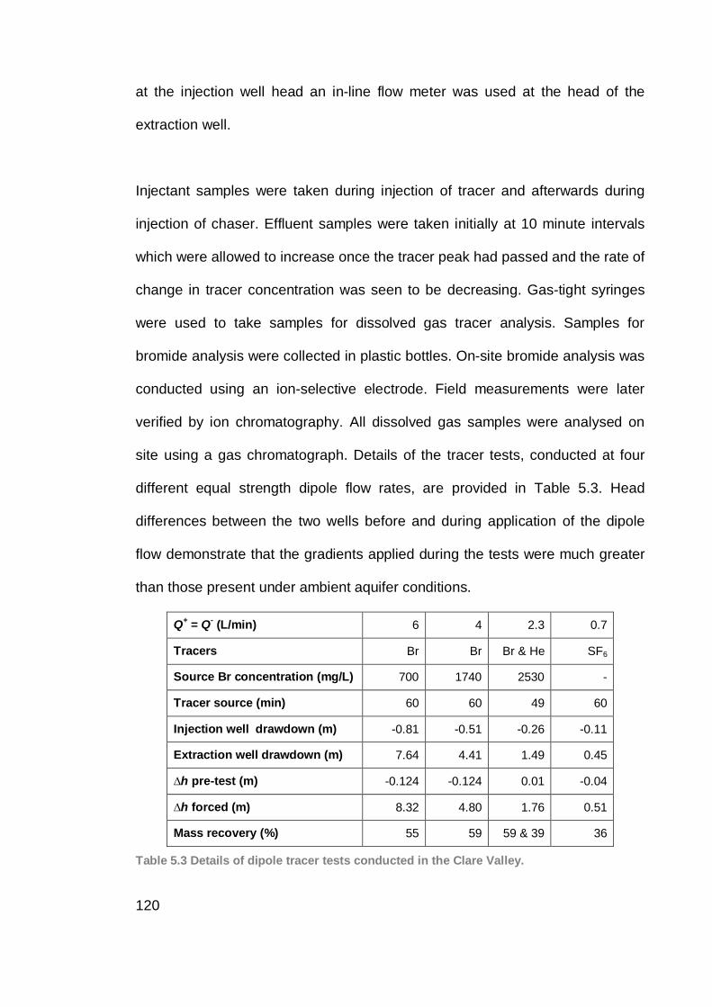
120

at the injection well head an in-line flow meter was used at the head of the

extraction well.

Injectant samples were taken during injection of tracer and afterwards during

injection of chaser. Effluent samples were taken initially at 10 minute intervals

which were allowed to increase once the tracer peak had passed and the rate of

change in tracer concentration was seen to be decreasing. Gas-tight syringes

were used to take samples for dissolved gas tracer analysis. Samples for

bromide analysis were collected in plastic bottles. On-site bromide analysis was

conducted using an ion-selective electrode. Field measurements were later

verified by ion chromatography. All dissolved gas samples were analysed on

site using a gas chromatograph. Details of the tracer tests, conducted at four

different equal strength dipole flow rates, are provided in Table 5.3. Head

differences between the two wells before and during application of the dipole

flow demonstrate that the gradients applied during the tests were much greater

than those present under ambient aquifer conditions.

Q+ = Q- (L/min) 6 4 2.3 0.7

Tracers Br Br Br & He SF6

Source Br concentration (mg/L) 700 1740 2530 -

Tracer source (min) 60 60 49 60

Injection well drawdown (m) -0.81 -0.51 -0.26 -0.11

Extraction well drawdown (m) 7.64 4.41 1.49 0.45

h pre-test (m) -0.124 -0.124 0.01 -0.04

h forced (m) 8.32 4.80 1.76 0.51

Mass recovery (%) 55 59 59 & 39 36

Table 5.3 Details of dipole tracer tests conducted in the Clare Valley.

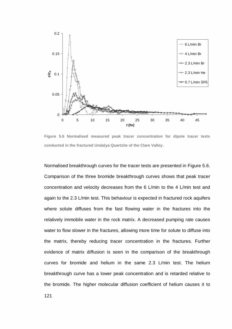
121

0

0.05

0.1

0.15

0.2

0 5 10 15 20 25 30 35 40 45

c/c 0

t (hr)

6 L/min Br

4 L/min Br

2.3 L/min Br

2.3 L/min He

0.7 L/min SF6

Figure 5.6 Normalised measured peak tracer concentration for dipole tracer tests

conducted in the fractured Undalya Quartzite of the Clare Valley.

Normalised breakthrough curves for the tracer tests are presented in Figure 5.6.

Comparison of the three bromide breakthrough curves shows that peak tracer

concentration and velocity decreases from the 6 L/min to the 4 L/min test and

again to the 2.3 L/min test. This behaviour is expected in fractured rock aquifers

where solute diffuses from the fast flowing water in the fractures into the

relatively immobile water in the rock matrix. A decreased pumping rate causes

water to flow slower in the fractures, allowing more time for solute to diffuse into

the matrix, thereby reducing tracer concentration in the fractures. Further

evidence of matrix diffusion is seen in the comparison of the breakthrough

curves for bromide and helium in the same 2.3 L/min test. The helium

breakthrough curve has a lower peak concentration and is retarded relative to

the bromide. The higher molecular diffusion coefficient of helium causes it to

122

diffuse more rapidly and further into the rock matrix than the bromide, thereby

experiencing greater effects of matrix diffusion.

Sanford et al. (2006) outline a methodology, based on hydraulic measurements,

for estimating the maximum tracer mass recovery that can be expected for a

tracer test between a well pair. The approach is based on apportioning flow that

goes into the injection well to fractures connecting the wells and fractures that

are connected to ‘elsewhere’ by their relative conductances. Using this

methodology conductances were determined to be 8.7 x 10-6 m2s-1 between the

well pair, 5.2 x 10-5 m2s-1 between the injection well and ‘elsewhere’ and 7.0 x

10-6 m2s-1 between the extraction well and ‘elsewhere’. A maximum expected

mass recovery of 58 % was calculated. Two factors dictate that all tracer sent

along fracture pathways connecting the two wells will never be recovered in a

real field setting. A dipole flow field creates some long flow paths along which

water and tracer movement is very slow and therefore it is not likely that this

tracer will be recovered within the duration of a tracer test. In addition, solute

that diffuses into the rock matrix is never fully recovered. Therefore the

theoretical maximum mass recovery is obtainable at infinite time, not within the

duration of an applied tracer test. Actual tracer mass recoveries for the tests

were 55 % of bromide at 6 L/min, 59 % of bromide at 4 L/min, 59 % of bromide

and 39 % of helium at 2.3 L/min and 36 % of SF6 at 0.7 L/min. The measured

values are generally consistent with the theoretically expected 58 %. Recovery

of helium was considerably lower than bromide in the 2.3 L/min test, as would

be expected in a system where matrix diffusion retards solute transport. Had the

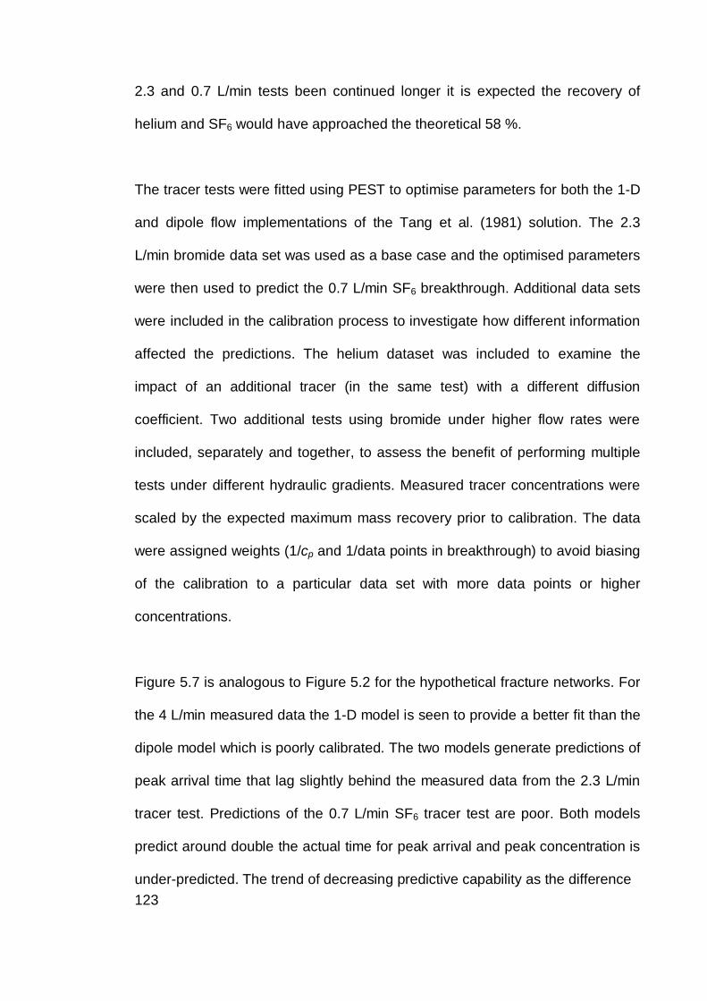
123

2.3 and 0.7 L/min tests been continued longer it is expected the recovery of

helium and SF6 would have approached the theoretical 58 %.

The tracer tests were fitted using PEST to optimise parameters for both the 1-D

and dipole flow implementations of the Tang et al. (1981) solution. The 2.3

L/min bromide data set was used as a base case and the optimised parameters

were then used to predict the 0.7 L/min SF6 breakthrough. Additional data sets

were included in the calibration process to investigate how different information

affected the predictions. The helium dataset was included to examine the

impact of an additional tracer (in the same test) with a different diffusion

coefficient. Two additional tests using bromide under higher flow rates were

included, separately and together, to assess the benefit of performing multiple

tests under different hydraulic gradients. Measured tracer concentrations were

scaled by the expected maximum mass recovery prior to calibration. The data

were assigned weights (1/cp and 1/data points in breakthrough) to avoid biasing

of the calibration to a particular data set with more data points or higher

concentrations.

Figure 5.7 is analogous to Figure 5.2 for the hypothetical fracture networks. For

the 4 L/min measured data the 1-D model is seen to provide a better fit than the

dipole model which is poorly calibrated. The two models generate predictions of

peak arrival time that lag slightly behind the measured data from the 2.3 L/min

tracer test. Predictions of the 0.7 L/min SF6 tracer test are poor. Both models

predict around double the actual time for peak arrival and peak concentration is

under-predicted. The trend of decreasing predictive capability as the difference

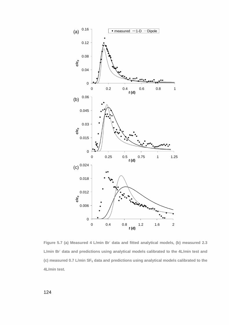
124

0

0.006

0.012

0.018

0.024

0 0.4 0.8 1.2 1.6 2

c/c 0

t (d)

0

0.015

0.03

0.045

0.06

0 0.25 0.5 0.75 1 1.25

c/c 0

t (d)

0

0.04

0.08

0.12

0.16

0 0.2 0.4 0.6 0.8 1

c/c 0

t (d)

measured 1-D Dipole(a)

(b)

(c)

Figure 5.7 (a) Measured 4 L/min Br- data and fitted analytical models, (b) measured 2.3

L/min Br- data and predictions using analytical models calibrated to the 4L/min test and

(c) measured 0.7 L/min SF6 data and predictions using analytical models calibrated to the

4L/min test.

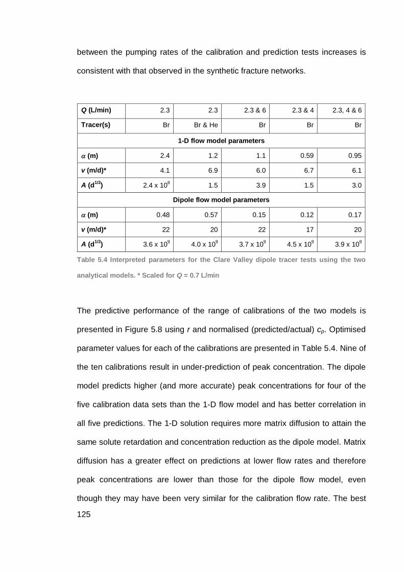
125

between the pumping rates of the calibration and prediction tests increases is

consistent with that observed in the synthetic fracture networks.

Q (L/min) 2.3 2.3 2.3 & 6 2.3 & 4 2.3, 4 & 6

Tracer(s) Br Br & He Br Br Br

1-D flow model parameters

(m) 2.4 1.2 1.1 0.59 0.95

v (m/d)* 4.1 6.9 6.0 6.7 6.1

A (d1/2) 2.4 x 108 1.5 3.9 1.5 3.0

Dipole flow model parameters

(m) 0.48 0.57 0.15 0.12 0.17

v (m/d)* 22 20 22 17 20

A (d1/2) 3.6 x 109 4.0 x 109 3.7 x 109 4.5 x 109 3.9 x 109

Table 5.4 Interpreted parameters for the Clare Valley dipole tracer tests using the two

analytical models. * Scaled for Q = 0.7 L/min

The predictive performance of the range of calibrations of the two models is

presented in Figure 5.8 using r and normalised (predicted/actual) cp. Optimised

parameter values for each of the calibrations are presented in Table 5.4. Nine of

the ten calibrations result in under-prediction of peak concentration. The dipole

model predicts higher (and more accurate) peak concentrations for four of the

five calibration data sets than the 1-D flow model and has better correlation in

all five predictions. The 1-D solution requires more matrix diffusion to attain the

same solute retardation and concentration reduction as the dipole model. Matrix

diffusion has a greater effect on predictions at lower flow rates and therefore

peak concentrations are lower than those for the dipole flow model, even

though they may have been very similar for the calibration flow rate. The best

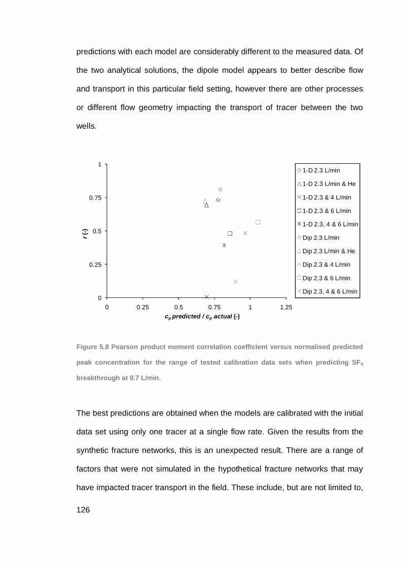
126

predictions with each model are considerably different to the measured data. Of

the two analytical solutions, the dipole model appears to better describe flow

and transport in this particular field setting, however there are other processes

or different flow geometry impacting the transport of tracer between the two

wells.

0

0.25

0.5

0.75

1

0 0.25 0.5 0.75 1 1.25

r(-)

cp predicted / cp actual (-)

1-D 2.3 L/min

1-D 2.3 L/min & He

1-D 2.3 & 4 L/min

1-D 2.3 & 6 L/min

1-D 2.3, 4 & 6 L/min

Dip 2.3 L/min

Dip 2.3 L/min & He

Dip 2.3 & 4 L/min

Dip 2.3 & 6 L/min

Dip 2.3, 4 & 6 L/min

Figure 5.8 Pearson product moment correlation coefficient versus normalised predicted

peak concentration for the range of tested calibration data sets when predicting SF6

breakthrough at 0.7 L/min.

The best predictions are obtained when the models are calibrated with the initial

data set using only one tracer at a single flow rate. Given the results from the

synthetic fracture networks, this is an unexpected result. There are a range of

factors that were not simulated in the hypothetical fracture networks that may

have impacted tracer transport in the field. These include, but are not limited to,

127

mixing in the plumbing and the wells, ambient groundwater flow in the aquifer,

density effects, dilation and contraction of fractures with hydraulic pressure,

residual tracer from previous tracer tests and saturation and desaturation of

fractures with the applied hydraulic gradients.

Discussion

Results from the hypothetical fracture networks indicated that including

additional information in the calibration of the two analytical models improved

predictions of solute transport under a reduced hydraulic gradient. However, the

predictions based on calibration to measured field data did not improve with

additional calibration data. The best predictions were obtained using only one

dataset, that with the lowest hydraulic gradient and therefore the most similar to

the predictive scenario. Of the wide range of factors that may have caused

variation between the theoretical and field observations, two were identified as

potentially significant; desaturation of fractures and residual tracer from

previous tests at the site.

The field tracer tests were conducted in an unconfined aquifer with

approximately 20 m of saturated aquifer above the well screens prior to

inducing the dipole flow fields. Injection and extraction at the two wells induced

hydraulic gradients between the wells that were different for each of the tests.

Data presented in Table 5.3 indicates that the hydraulic head difference

between the two wells varied between 0.51 and 8.32 m for the five tests. The

majority of the head differences was generated by drawdown at the extraction

well. Drawdown of 7.64 m was observed for the 6 L/min test, reducing the

128

saturated thickness of the aquifer near the well by almost 40 %. Whilst it isn’t

known what proportion of the previously active fracture pathways between the

wells were desaturated by the imposed dipole flow field, it is likely that it was

significant. The relationship between drawdown and pumping rate was greater

than linear, indicating that conductive fractures were being desaturated. Given

the hydraulic results, it is evident that tests conducted at different pumping rates

were each sampling a different network of active fractures. Therefore the

addition of tracer data for tests at higher pumping rates may bias the calibration

process to a different interpretation of aquifer parameters that is not

representative of the active fracture network for the 0.7 L/min test being

predicted. In this scenario it is quite conceivable that the inclusion of tracer data

for higher pumping rates in the calibration process could lead to a decrease in

predictive performance. This helps explain why the addition of data from the 6

L/min and 4L/min tests to that of the 2.3 L/min lead to worse predictions of the

0.7 L/min SF6 tracer breakthrough. However, addition of the 4 L/min data

worsened predictions more than when the 6 L/min data was included, even

though the network of active fractures would have been more similar to that in

the predicted test.

It is likely that each of the tests was impacted to a varying degree by residual

tracer in the aquifer from previous tests. Two tests using bromide were

conducted prior to any of the tests presented in this study and then each of the

bromide tests presented here left tracer in the aquifer. In order to account for

any background bromide in the aquifer, samples of the ambient groundwater

were taken before each of the tests and this concentration was subtracted from

129

those measured at the extraction well during the test. This was deemed the best

approach to account for the residual tracer, but it is a simplification as the

bromide concentration will not have been uniform throughout the aquifer prior to

each test. The build-up of background bromide was the reason for using SF6 in

the final, lowest gradient test. The SF6 and helium data sets were not impacted

by any previous tracer tests at the site. Of the tests using bromide presented in

this study, the 6 L/min test was carried out first, followed by the 4 L/min and 2.3

L/min tests. The background bromide concentration at the site prior to carrying

out any tests was around 2 mg/L. Prior to the 6 L/min test it had increased to 35

mg/L then further to 40.5 mg/L before the 4 L/min test. Background bromide had

decreased considerably to 19 mg/L by the time the 2.3 L/min test was

conducted. Based on this information it is expected that the simple process

used to account for background tracer would have the greatest consequences

in interpreting the 4 L/min test, followed by the 6 L/min test then the 2.3 L/min

test. Therefore the residual bromide present in the aquifer may explain why the

predictions made using the 6 L/min data were superior to those using the 4

L/min data, despite the latter inducing a hydraulic gradient (and associated

active fractures) more similar to that of the 0.7 L/min prediction. It is not clear

why the inclusion of the helium data did not improve predictions.

Conclusions

This study has examined the ability of two analytical models to predict solute

transport in fracture networks when calibrated to tracer test data. Dipole tracer

tests were simulated in three hypothetical fracture networks and a series of field

130

tracer tests were conducted in the Clare Valley, South Australia. Key findings

can be summarised as follows:

1) Whilst not being exact descriptions of flow in a fracture network, the 1-D

flow and dipole flow models could each be calibrated to generate a good

fit to the measured data. The suitability of the analytical models could

only be determined when they were calibrated to one data set and used

to predict another data set under different conditions. Multiple tracer data

sets should be obtained when characterising a field site to enable

identification of a suitable interpretive model.

2) Predictions of solute transport were more accurate when calibrated to

measured tracer data than when parameters were assigned values

based on hydraulic data and averaged fracture properties.

3) For the hypothetical fracture networks, inclusion of additional data sets in

the calibration process resulted in better predictions. The most useful

additional data was that obtained at a lower hydraulic gradient, closer to

that of the prediction. Field confirmation of these results in a confined

fractured rock aquifer would be useful.

4) Predictions of the field dipole tracer test conducted at the lowest pumping

rate were not improved by including additional data sets in the

calibration process.

5) In shallow unconfined aquifers the desaturation of the fracture pathways

between a well pair with increased dipole strength can result in poor

characterisation of solute transport under lower hydraulic gradients. If

hydraulic testing indicates significant dewatering of the aquifer near the

131

extraction well tests should be conducted at the lowest practical dipole

strengths.

132

Notation and Units

Subscript f denotes a fracture property.

ai area associated with fracture node L2



c solute concentration in the Laplace space TML-3


cmax specified maximum concentration change

per time-step ML-3

cp peak concentration ML-3




h hydraulic head L

K hydraulic conductivity LT-1

Lw well screen length L

mx grid spacing multiplier in the x direction -

n integer element counter -

p Laplace space variable T-1

Q injection or extraction rate L3T-1

rw well radius L

r Pearson product moment correlation coefficient -


133


t time T


Vi region or control volume associated with

porous medium node i L3

vpr prediction water velocity / test water velocity -

x, y, z spatial coordinates L

X, Y, Z model domain size in x, y and z directions L

L longitudinal dispersivity L

T transverse dispersivity L

VT vertical transverse dispersivity L

ij describes fluid flow between i and j L2T-1

finite difference time weighting factor -

porosity -


tortuosity -

ij describes diffusive/dispersive solute flux

between i and j L3T-1

solute exchange rate between domains T-1

134

References



Grove, D.B. and Beetem, W.A., 1971. Porosity and dispersion constant

calculations for a fractured carbonate aquifer using the two well tracer method.

Water Resources Research, 7(1): 128-134.

Himmelsbach, T., Hotzl, H. and Maloszewski, P., 1998. Solute transport

processes in a highly permeable fault zone of Lindau fractured rock test site

(Germany). Ground Water, 36(5): 792-800.

Himmelsbach, T. and Maloszewski, P., 1992. Tracer tests and hydraulic

investigations in the observation tunnel Lindau. Steirische Beitraege zur

Hydrogeologie: 197-228.

Novakowski, K.S., 1988. Comparison of fracture aperture widths determined

from hydraulic measurements and tracer experiments. In: B. Hitchon and S.

Bachu (Editors), Proceedings: 4th Canadian/American Conference on

Hydrogeology. National Water Well Association, Dublin, Ohio, pp. 68-80.

Novakowski, K.S., Bickerton, G. and Lapcevic, P., 2004. Interpretation of

injection-withdrawal tracer experiments conducted between two wells in a large

single fracture. Journal of Contaminant Hydrology, 73: 227-247.




135

Pfingsten, W. and Soler, J.M., 2003. Modelling of nonreactive tracer dipole tests

in a shear zone at the Grimsel test site. Journal of Contaminant Hydrology, 61:

387-403.



Transactions on Mathematical Software, 10(3): 348-353.



Adelaide.



Sanford, W.E., Cook, P.G., Robinson, N.I. and Weatherill, D., 2006. Tracer

mass recovery in fractured aquifers estimated from multiple well tests. Ground

Water.




Therrien, R., Sudicky, E.A., McLaren, R.G. and Panday, S.M., 2005.

HydroGeoSphere: A three-dimensional numerical model describing fully-

integrated subsurface and surface flow and solute transport. User's Guide,

Groundwater Simulations Group, Waterloo, Canada.

Weatherill, D. et al., 2008. Discretizing the fracture-matrix interface to simulate

solute transport. Ground Water, 46(4): 606-615.

Webster, D.S., Proctor, J.F. and Marine, I.W., 1970. Two-well tracer test in

fractured crystalline rock. US Geological Survey Water Supply Paper, 1544-I.

136

Chapter 6: Concluding Remarks

Summary of Findings

Through a combination of analytical modelling, numerical modelling and

implementation of field tracer tests, the research carried out in this thesis has

delivered new scientific knowledge regarding the use of applied tracer tests to

predict solute transport in fractured rock. In so doing, the thesis has met its

stated objectives which are to:

1) evaluate how accurately aquifer parameters can be determined from

tracer test data, given the inability of analytical models to completely

describe the complex nature of fractured rock and associated tracer

breakthrough curves;

2) quantify the impact of parameter and interpretative model uncertainty on

predictions of solute transport under lower hydraulic gradients;

3) identify the most effective ways to improve the accuracy of predictions of

solute transport in fractured rock aquifers made using tracer test data;

Chapter 2 demonstrates that, when ‘accepting’ a number of analytical

interpretations of a breakthrough curve (all using the same model) non-

uniqueness associated with individual parameters can become significant.

However, results show that predictions of breakthrough curve characteristics

(first inflection point time, peak arrival time and peak concentration) for

groundwater flow speeds orders of magnitude smaller than that at which a test

137

is conducted can sometimes be determined even more accurately than the

fracture and matrix parameters.

Chapter 4 takes the ideas behind Chapter 2 a step further to examine the non-

uniqueness introduced when two different analytical flow models are considered

in the interpretation of a dipole tracer test. Results demonstrate that the two

models can produce almost identical breakthrough curves for a range of

scenarios. However, in order to do so, sometimes very different and conflicting

interpreted aquifer parameter values are required in order to produce the same

tracer breakthrough. The study demonstrates the importance of incorporating

multiple conceptual models in the analyses of dipole tracer tests conducted in

fractured rock, where the actual flow geometry may be poorly understood.

Chapter 5 builds on the outcomes of Chapter 4, using two different analytical

models to interpret breakthrough curves and then subsequently predict

transport under lower hydraulic gradients. This is done firstly with breakthrough

curves generated by simulating dipole tracer tests in hypothetical 3-D fracture

networks for which the characteristics were known, and secondly, with

breakthrough curves obtained by carrying out dipole tracer tests in the field.

Several approaches to reducing predictive uncertainty are tested. The most

effective method is to carry out an additional test at a lower injection and

extraction rate. In practice this suggests that, when the aim of a tracer test is to

enable prediction of transport under ambient flow conditions, the test should be

carried out under the lowest feasible imposed hydraulic gradient.

138

Chapter 3 is a by-product of some of the work carried out in Chapter 5, which

involved simulating tracer transport in fractured networks between a dipole well

pair. The study examines the required spatial discretisation perpendicular to the

FMI for numerical simulation of solute transport in discretely-fractured porous

media. To match analytical results on the relatively short timescales simulated

in the study, very fine grid spacing perpendicular to the FMI, of the scale of the

fracture aperture, is necessary if advection and/or dispersion in the fracture are

high compared to diffusion in the matrix. The requirement of such extremely fine

spatial discretisation has not been previously reported in the literature. In cases

of high matrix diffusion, matching the analytical results is achieved with larger

grid spacing at the FMI. Cases where matrix diffusion is lower can employ a

larger grid multiplier moving away from the FMI.

Further Research

This thesis has tackled some of the issues associated with using applied tracer

tests to predict solute transport in fractured rock, but other aspects remain to be

addressed. The following section outlines areas where further research is

warranted.

The up-scaling of interpreted aquifer properties from an applied tracer test,

sampling a particular portion of aquifer, to the aquifer more generally is an issue

that warrants further attention. Whilst applied tracer tests can be designed to

sample differing volumes of aquifer, the reality is that most tests will be

conducted over shorter intervals, and sample lesser volumes of aquifer, than

that over which predictions are made. The act of applying test-scale results to

139

the broader aquifer, necessarily assumes that the test has been carried out over

a sample of aquifer greater than the representative elementary volume (REV). A

combination of field-based and modelling studies could be used to investigate

this issue. Activities might include carrying out/simulating tests at different

locations and over different scales within a fractured rock aquifer.

A similar issue concerns the anisotropy inherent in most fractured rock aquifers.

Generally, the fracturing in the rock will create anisotropy in bulk hydraulic

conductivity. A study could focus on the use of applied tracer tests to investigate

anisotropy and how it varies with spatial scale.

This study examined the uncertainties associated with parameters and

predictions when using single fracture models to investigate both field derived

and numerically simulated breakthrough curves. The numerical simulations of

transport in 3-D fracture networks were numerically cumbersome which limited

the number of networks that were simulated. However, with ever-increasing

computational capabilities, particularly recent advances in parallel and could

computing, the time and memory demands for simulating solute transport in 3-

D fracture networks are becoming less burdensome. This opens the door to the

use of stochastic modelling approaches for investigating tracer behaviour in 3-D

fracture networks. Stochastic modelling, through its ability to deliver probabilistic

outcomes, has the potential to provide insights into the characteristics of

networks in which tracer transport can be reasonably approximated by single

fracture analytical solutions and those that require representation of discrete

fracture sets or fractures.

140

Similarly, the use of stochastic modelling techniques could allow investigation of

the linkages between network geometry and the most appropriate analytical

solution for describing flow geometry. This thesis has made initial comparisons

between interpretations with 1-D and dipole flow analytical models. The

applicability of these, and additional flow geometries, could be investigated for

appropriately chosen network geometry classifications.

141

Appendix A: Published Papers

142

143

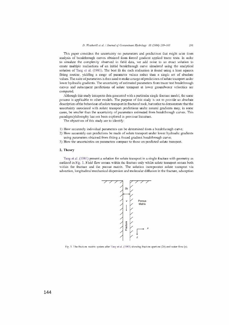
144

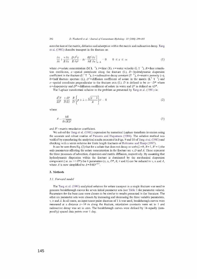
145

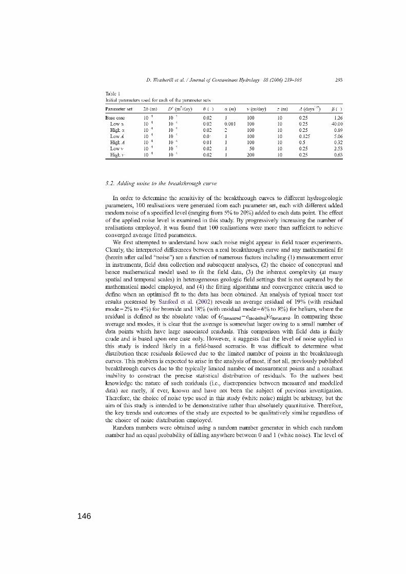
146

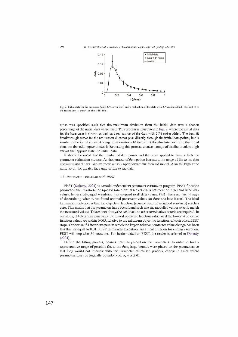
147

148

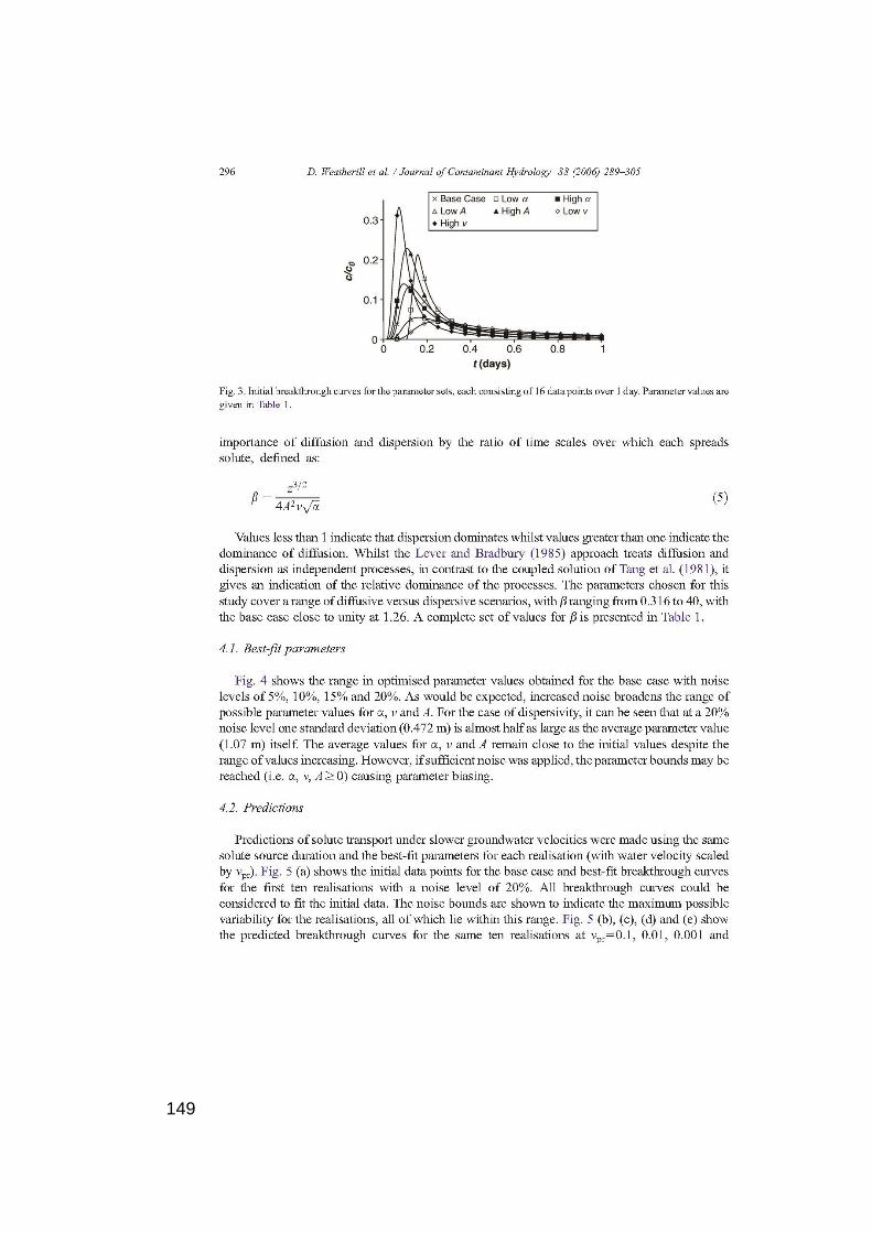
149

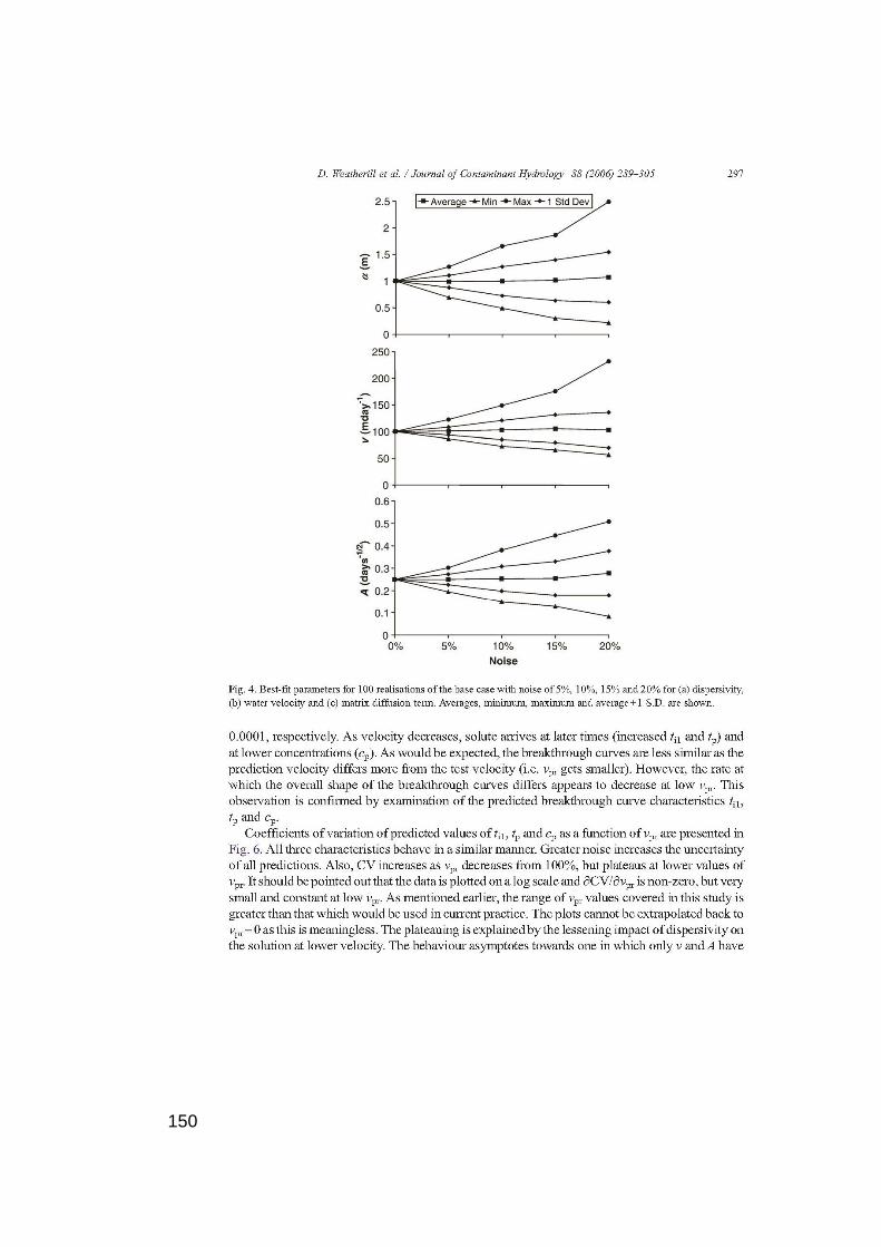
150

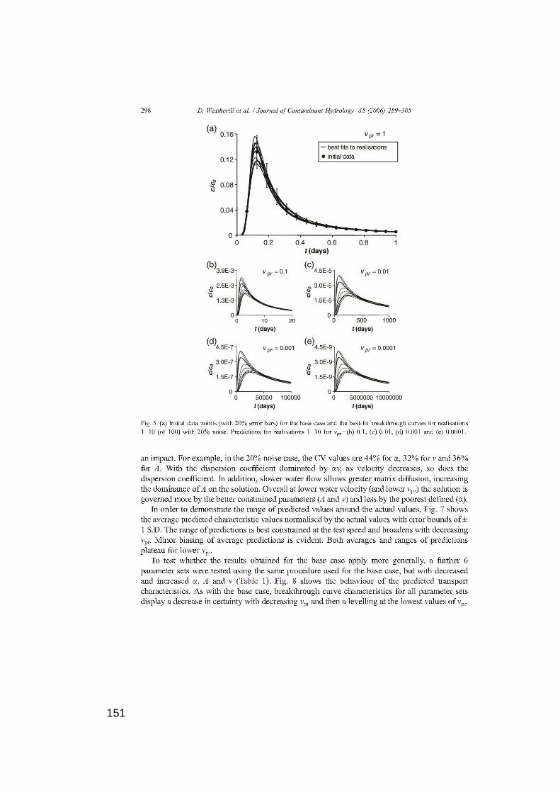
151

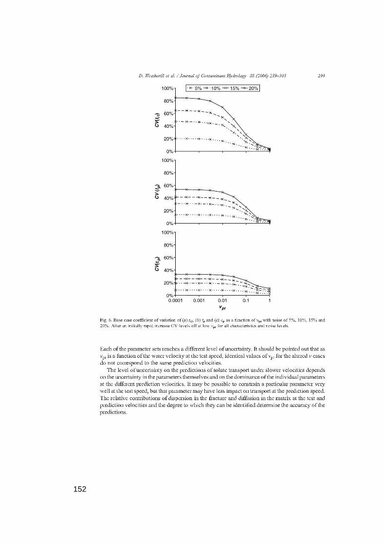
152

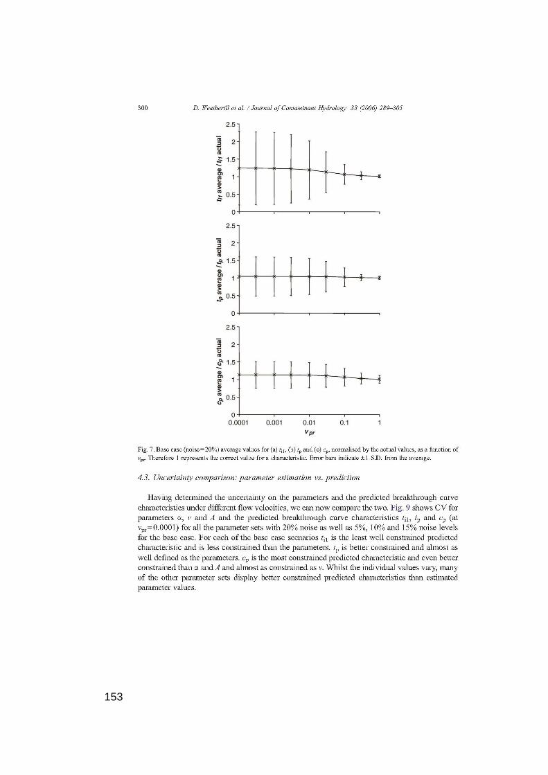
153

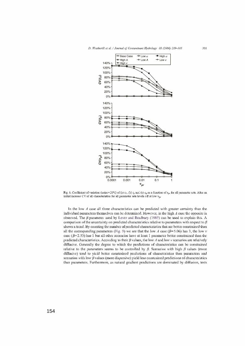
154

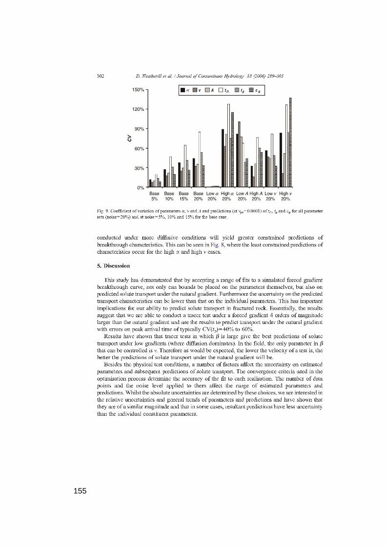
155

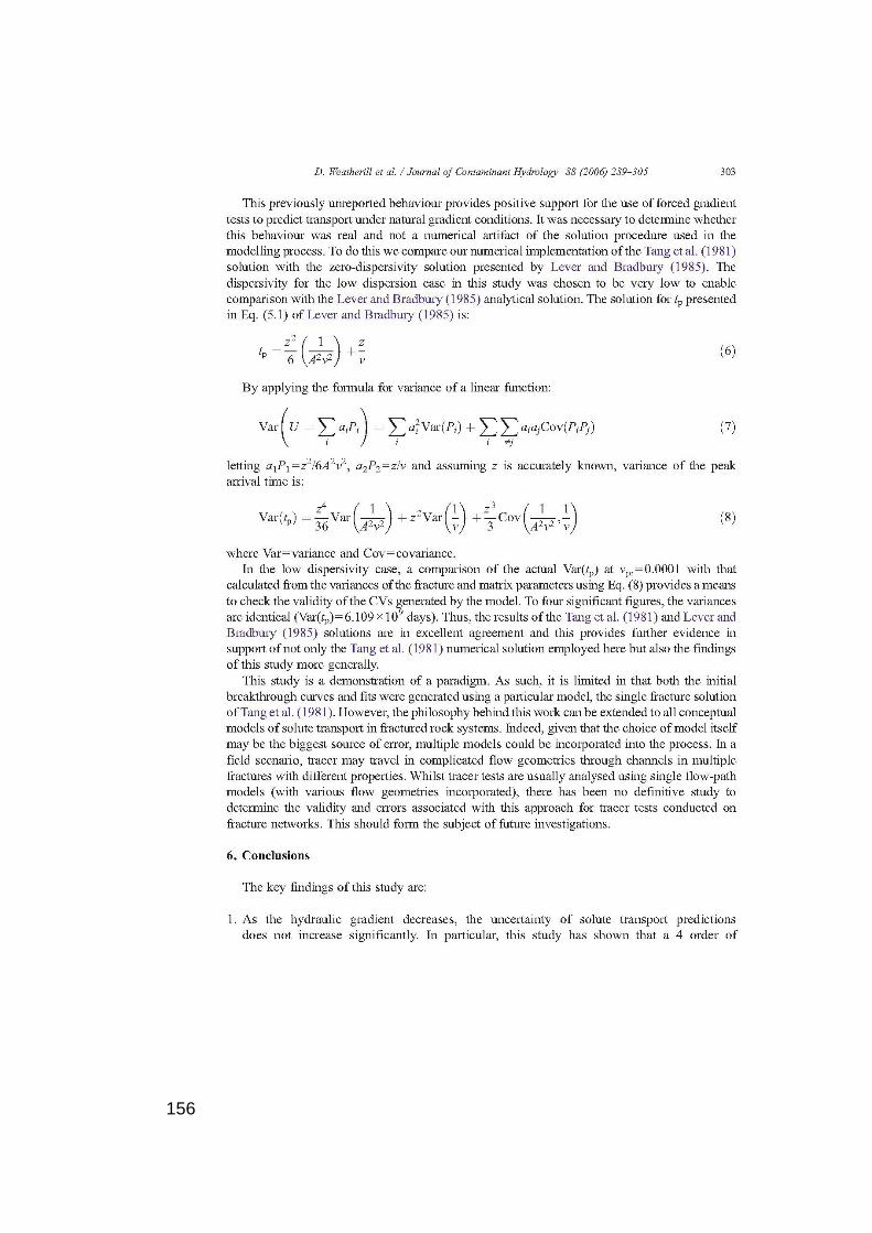
156

157

158

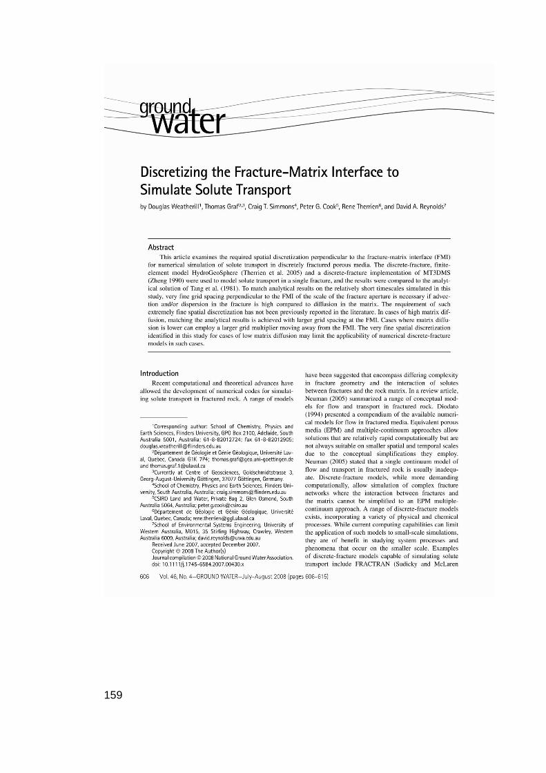
159

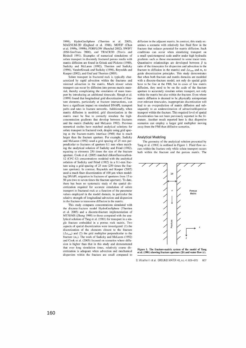
160

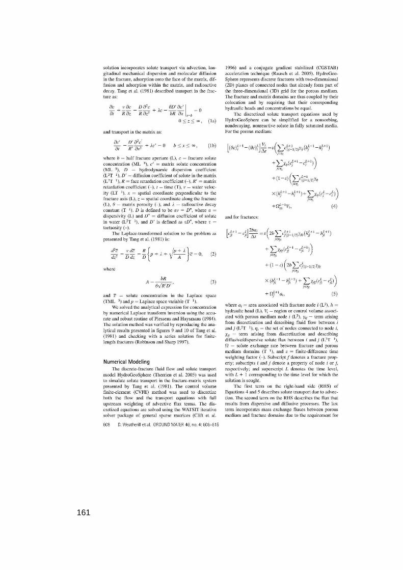
161

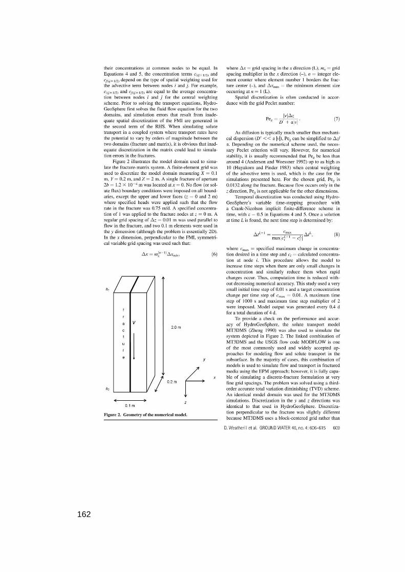
162

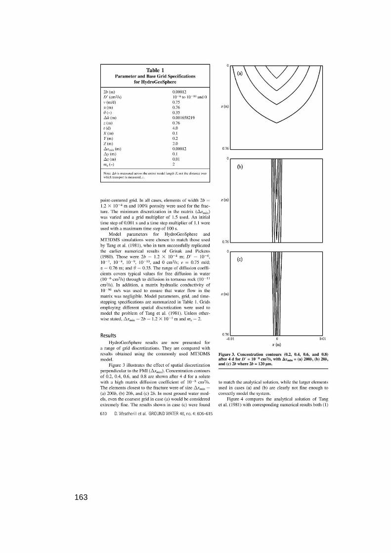
163

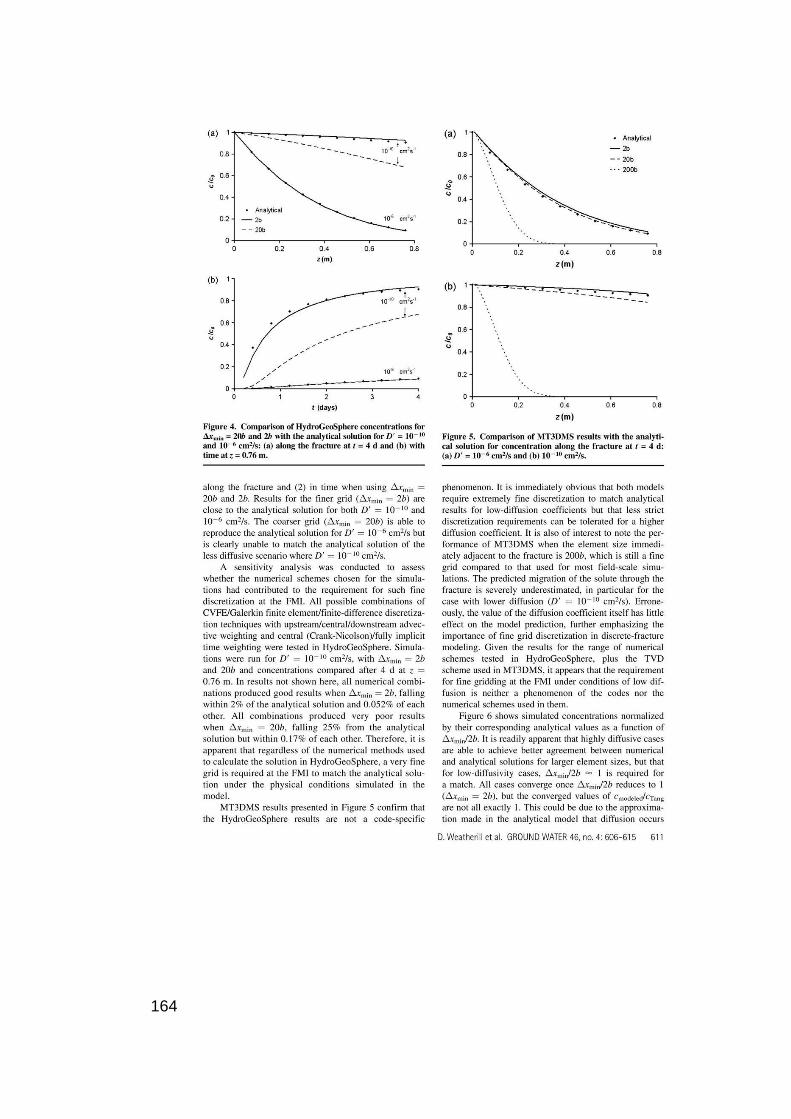
164

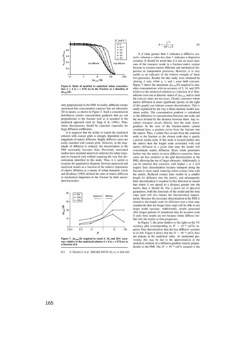
165

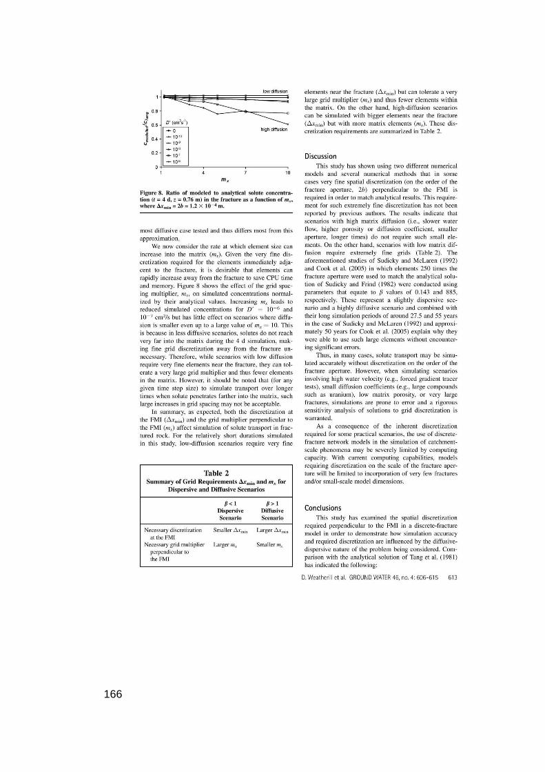
166

167

168

Documents

Using applied tracer tests to predict solute transport in - Theses