Embed Size (px)
Citation preview
S1
Using Cavitation Rheology to Understand Dipeptide-Based
Gels
Ana M. Fuentes-Caparrós,a Bart Dietrich,a Lisa Thomson,a Charles Chauveaua,b and Dave J. Adamsa,*
a School of Chemistry, University of Glasgow, Glasgow, G12 8QQ, U.K.
E-mail: [email protected]
b Department of Chemistry, University of Mans, Mans, Avenue Olivier Messiaen 72085, France.
Supporting Information
Section I
Experimental S2
Supplementary Figures S4
References S17
Section II. CRAB v0.1 and CRAB Control v0.1 Manual
Section II.1. Hardware Manual S21
Section II.2. Operating Principles S37
Section II.3. CRAB Control v0.1 Software Manual S49
Electronic Supplementary Material (ESI) for Soft Matter.This journal is © The Royal Society of Chemistry 2019
S2
Section I
Experimental
Materials
PVA (poly(vinyl alcohol)) hydrogels. PVA hydrogels were prepared as
described before1. A 13,000-23,000 Mw and 98 % hydrolysed polymer was heated
at 90 °C in a solution containing DMSO:water in a 40:60 ratio and 2% boric acid
was added as a cross-linking agent. This solution was heated overnight and left
the solution to cool down at room temperature to form a gel. All samples were made
of 10% PVA.
Gelatine. Gelatine hydrogels were made from a beef gelatine powder supplied by
Dr. Oetker. Water was added to the gelatine powder and heated at 50 °C for 1 hour.
Then solution was left to cool down and form the gel.
LMWG: Dipeptides FmocLG and 2NapFF were synthesised as described
previously.2-3 All other materials were purchased from Sigma Aldrich.
Samples preparation
Solvent-Triggered Gelation. Stock solutions of gelator were prepared at different
concentrations by dissolving the weighed gelator in DMSO. Upon complete
dissolution of the gelator, distilled water was added to make the sample up to a
final volume of 2 mL gel. The volume of DMSO and water used varied depending
on the final ɸDMSO desired. The sample was then left to gel overnight before analysis.
pH-Triggered Gelation. A stock solution of each gelator was prepared at different
concentrations by weighing the required amount of gelator and adding dilute
sodium hydroxide solution (1 molar equivalent of a 0.1 M solution) and water and
stirring until fully dissolved. The gelator stock solution was added to a pre-weighed
amount of glucono-δ-lactone, GdL (3 molar equivalents of GdL for each equivalent
of gelator) and gently shaken to dissolve all GdL. The sample was left to stand to
allow gelation to occur overnight (~ 18 hours).
Experimental Details
Oscillatory Shear Rheology.
All rheological measurements were performed using Anton Paar Physica MCR
101 and MCR 301 rheometers. A cup and vane system was used to perform
frequency sweeps. 2mL gels were prepared in 7 mL Sterilin vials and left overnight
(~ 18 hours) at room temperature to gel before measurements. Frequency sweeps
were performed at 25 °C in a range of frequencies from 1 to 100 rad s-1 at a
constant strain of 0.5 % to ensure being within the linear viscoelastic (LVE) region.
The storage moduli (G') at 10 rad s-1 was used to compare with the maximum

S3
pressure, Pc, obtained with the cavitation rheology. All measurements were
repeated three times to ensure reproducibility.
Cavitation Rheology.
Cavitation experiments were carried out using a lab-built instrument. It includes a
syringe pump (World Precision Instruments AL-1000) assembled into a 10 mL
HamiltonTM 1000 series Gastight syringe for air pumping. A high precision
manometer “CRAB (Cavitation Rheology Analyser Box)” with data logging
capability was custom-built to control and record the pressure. A digital
manometer was connected into the system via Y-junction and used to calibrate
and double check pressure readings from the CRAB. The air rate pumped was 0.4
mL min-1 and a needle gauge 22 was used (~ 413 µm inner diameter). A
conductivity probe controls the needle immersion depth by sending a signal to an
3D printer, which allows to precise positioning the needle below the surface of the
sample.
Confocal microscopy.
Confocal images were taken using a Zeiss LSM 710 confocal microscope with a
LD EC Epiplan NEUFLUAR 50X (0,55 DIC) objective. All samples were prepared
in a Greiner Bio-One CELLviewTM 35 mm plastic cell culture dish with a
borosilicate glass bottom. Fluorescence from Nile Blue was excited using a 634
nm He-Ne laser and emission was detected between 650 and 710 nm. Samples
were prepared in-situ, using the methodology described below. All gels triggered
using a solvent switch were stained with a 0.1 wt% Nile Blue solution. The Nile
Blue was added to the DMSO-gelator solution to a final Nile Blue concentration of
2 µL mL-1. To stain the pH switched samples a 0.1 wt% Nile Blue solution was
prepared and added to the gelator solution to a final Nile Blue concentration of 2
µL mL-1.
S4
Supplementary Figures
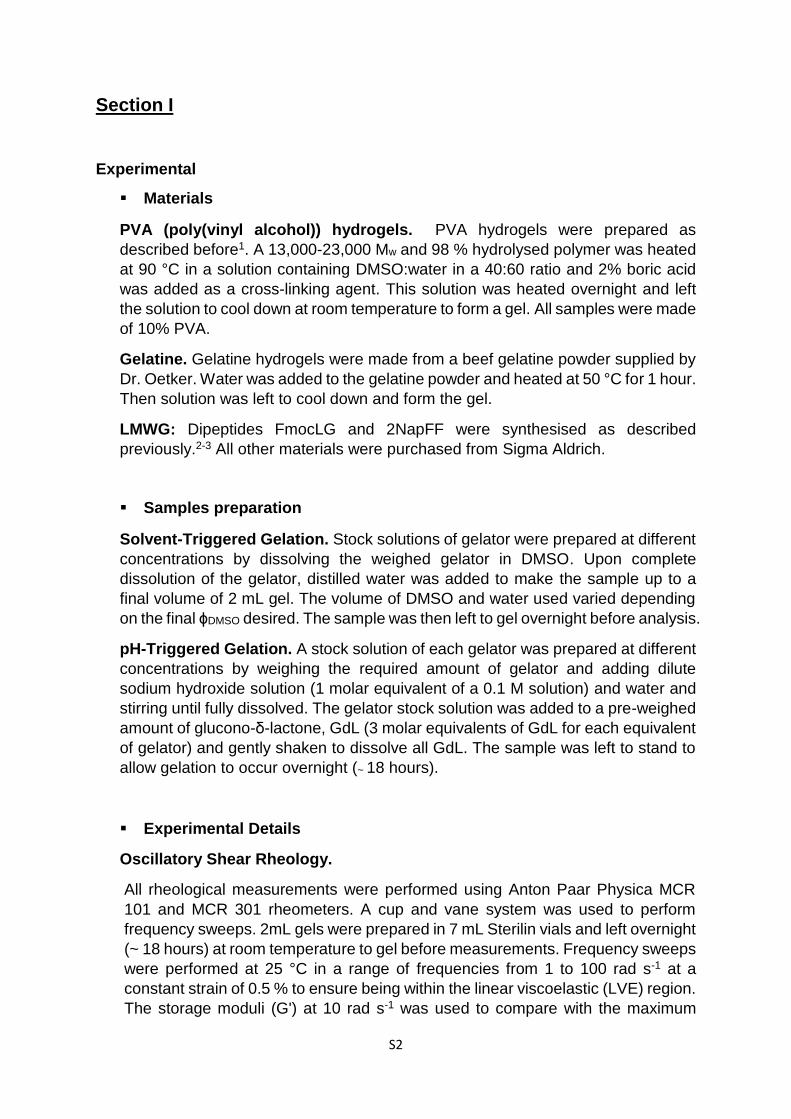
Figure S1. Critical pressure, Pc, as a function of depth within the material for gel 1 using a
solvent switch to trigger gelation. Error bars represent three measurements at each depth to
ensure reproducibility.
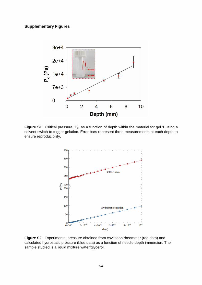
Figure S2. Experimental pressure obtained from cavitation rheometer (red data) and
calculated hydrostatic pressure (blue data) as a function of needle depth immersion. The
sample studied is a liquid mixture water/glycerol.

S5
Figure S3. Cavitation data for gelatine at (a) 10 mg mL-1; (b) 20 mg mL-1; (c) 30 mg mL-1; (d)
40 mg mL-1; (e) 50 mg mL-1; (f) 60 mg mL-1; (g) 70 mg mL-1; (h) 80 mg mL-1; (i) 90 mg mL-1; (j)
100 mg mL-1; (k) 110 mg mL-1 and (l) 120 mg mL-1.
S6
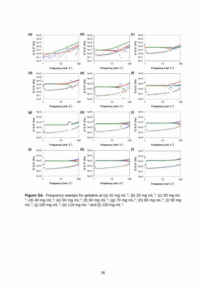
Figure S4. Frequency sweeps for gelatine at (a) 10 mg mL-1; (b) 20 mg mL-1; (c) 30 mg mL-
1; (d) 40 mg mL-1; (e) 50 mg mL-1; (f) 60 mg mL-1; (g) 70 mg mL-1; (h) 80 mg mL-1; (i) 90 mg
mL-1; (j) 100 mg mL-1; (k) 110 mg mL-1 and (l) 120 mg mL-1.

S7
Figure S5. Frequency sweeps for PVA gels at (a) day 1; (b) day 2; (c) day 3; (d) day 4; (e)
day 5; (f) day 6; (g) day 7; (h) day 8; (i) day 9; (j) day 10; (k) day 12 and (l) day 15 after being
synthesised.
S8
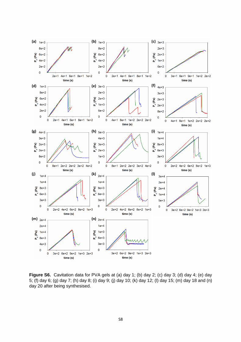
Figure S6. Cavitation data for PVA gels at (a) day 1; (b) day 2; (c) day 3; (d) day 4; (e) day
5; (f) day 6; (g) day 7; (h) day 8; (i) day 9; (j) day 10; (k) day 12; (l) day 15; (m) day 18 and (n)
day 20 after being synthesised.
S9
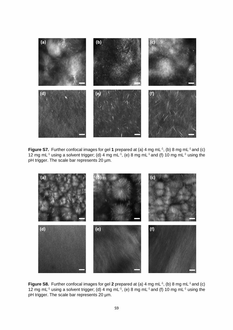
Figure S7. Further confocal images for gel 1 prepared at (a) 4 mg mL-1, (b) 8 mg mL-1 and (c)
12 mg mL-1 using a solvent trigger; (d) 4 mg mL-1, (e) 8 mg mL-1 and (f) 10 mg mL-1 using the
pH trigger. The scale bar represents 20 µm.
Figure S8. Further confocal images for gel 2 prepared at (a) 4 mg mL-1, (b) 8 mg mL-1 and (c)
12 mg mL-1 using a solvent trigger; (d) 4 mg mL-1, (e) 8 mg mL-1 and (f) 10 mg mL-1 using the
pH trigger. The scale bar represents 20 µm.
S10
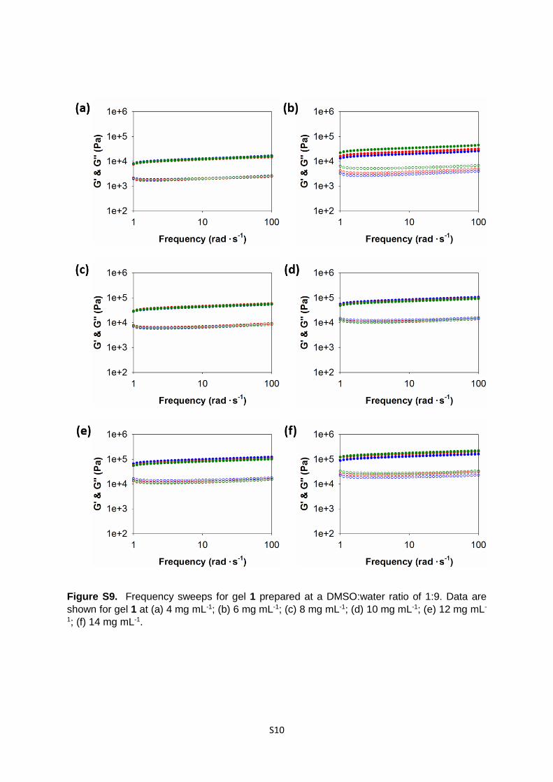
Figure S9. Frequency sweeps for gel 1 prepared at a DMSO:water ratio of 1:9. Data are
shown for gel 1 at (a) 4 mg mL-1; (b) 6 mg mL-1; (c) 8 mg mL-1; (d) 10 mg mL-1; (e) 12 mg mL-
1; (f) 14 mg mL-1.
S11
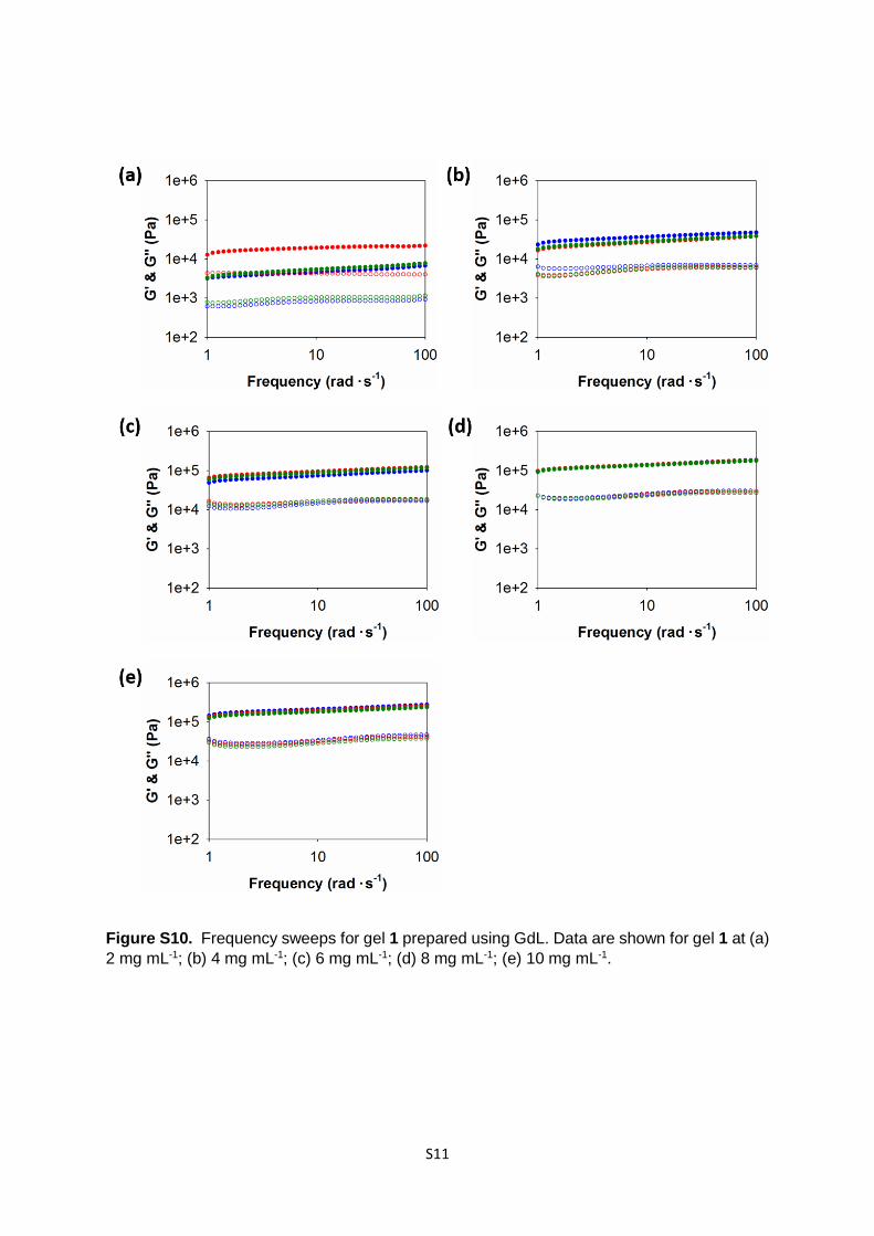
Figure S10. Frequency sweeps for gel 1 prepared using GdL. Data are shown for gel 1 at (a)
2 mg mL-1; (b) 4 mg mL-1; (c) 6 mg mL-1; (d) 8 mg mL-1; (e) 10 mg mL-1.
S12
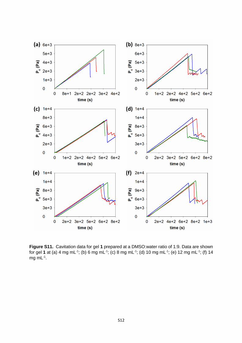
Figure S11. Cavitation data for gel 1 prepared at a DMSO:water ratio of 1:9. Data are shown
for gel 1 at (a) 4 mg mL-1; (b) 6 mg mL-1; (c) 8 mg mL-1; (d) 10 mg mL-1; (e) 12 mg mL-1; (f) 14
mg mL-1.
S13
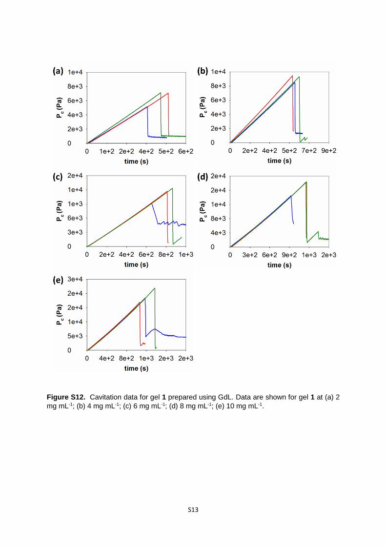
Figure S12. Cavitation data for gel 1 prepared using GdL. Data are shown for gel 1 at (a) 2
mg mL-1; (b) 4 mg mL-1; (c) 6 mg mL-1; (d) 8 mg mL-1; (e) 10 mg mL-1.
S14
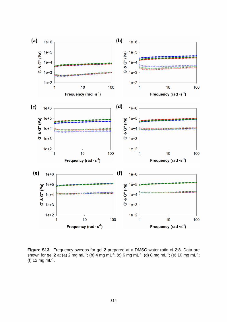
Figure S13. Frequency sweeps for gel 2 prepared at a DMSO:water ratio of 2:8. Data are
shown for gel 2 at (a) 2 mg mL-1; (b) 4 mg mL-1; (c) 6 mg mL-1; (d) 8 mg mL-1; (e) 10 mg mL-1;
(f) 12 mg mL-1.
S15
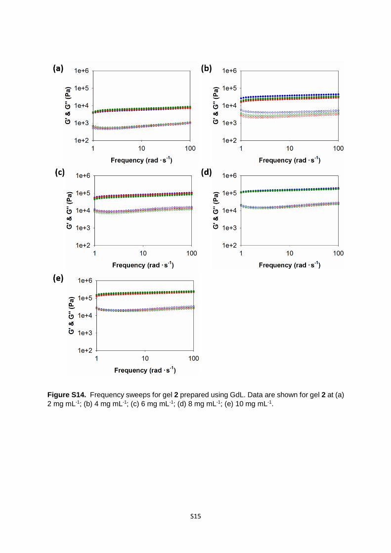
Figure S14. Frequency sweeps for gel 2 prepared using GdL. Data are shown for gel 2 at (a)
2 mg mL-1; (b) 4 mg mL-1; (c) 6 mg mL-1; (d) 8 mg mL-1; (e) 10 mg mL-1.
S16
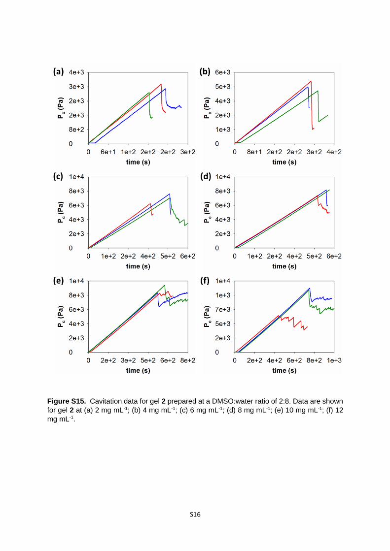
Figure S15. Cavitation data for gel 2 prepared at a DMSO:water ratio of 2:8. Data are shown
for gel 2 at (a) 2 mg mL-1; (b) 4 mg mL-1; (c) 6 mg mL-1; (d) 8 mg mL-1; (e) 10 mg mL-1; (f) 12
mg mL-1.
S17
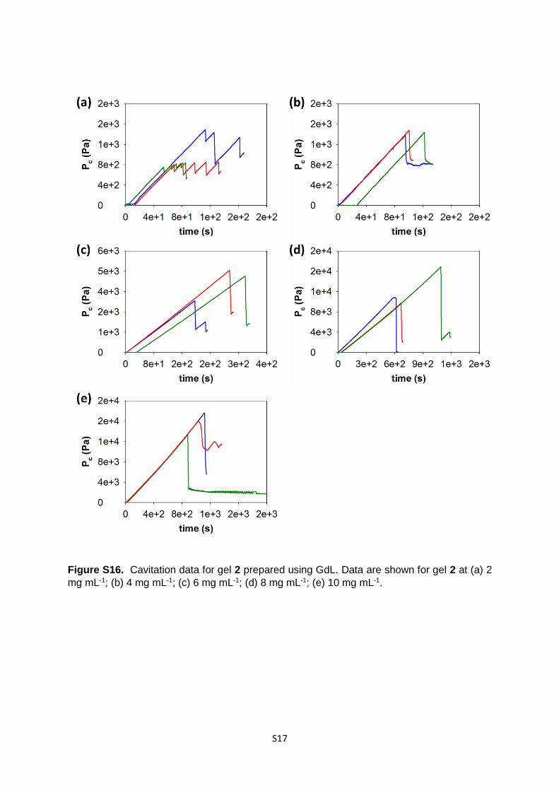
Figure S16. Cavitation data for gel 2 prepared using GdL. Data are shown for gel 2 at (a) 2
mg mL-1; (b) 4 mg mL-1; (c) 6 mg mL-1; (d) 8 mg mL-1; (e) 10 mg mL-1.
S18
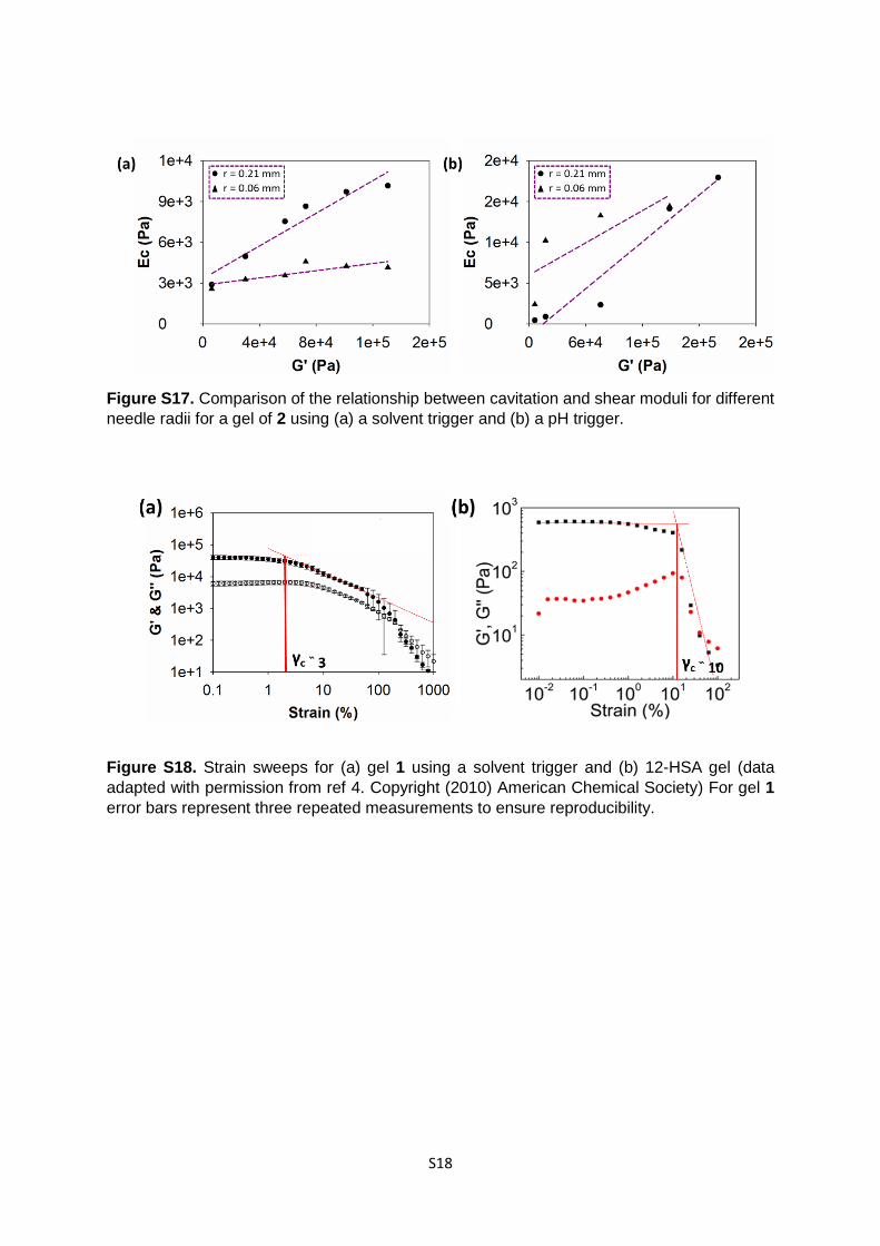
Figure S17. Comparison of the relationship between cavitation and shear moduli for different
needle radii for a gel of 2 using (a) a solvent trigger and (b) a pH trigger.
Figure S18. Strain sweeps for (a) gel 1 using a solvent trigger and (b) 12-HSA gel (data
adapted with permission from ref 4. Copyright (2010) American Chemical Society) For gel 1
error bars represent three repeated measurements to ensure reproducibility.

S19
Figure S19. Strain sweeps for (a) gel 1 using a solvent trigger, (b) gel 1 using a pH trigger, (c)
gel 2 using a solvent trigger, (d) gel 2 using a pH trigger, (e) gelatine and (f) PVA-borax gel.
The intersection between the linear-viscoelastic region and the section from where G' and G''
start to deviate from linearity represent the critical strain, γc. Gels (a-d) at 6 mg mL-1, gelatine
at 60 mg mL-1 and PVA-borax gel 5 days after synthesis.
References
1. A. Samzadeh-Kermani, M. Mirzaee and M. Ghaffari-Moghaddam, Advances in Biological Chemistry, 2016, DOI: 10.4236/abc.2016.61001, 1-11.
2. D. J. Adams, L. M. Mullen, M. Berta, L. Chen and W. J. Frith, Soft Matter, 2010, 6, 1971-1980. 3. L. Chen, S. Revel, K. Morris, L. C. Serpell and D. J. Adams, Langmuir, 2010, 26, 13466-13471. 4. P. Fei, S. J. Wood, Y. Chen and K. A. Cavicchi, Langmuir, 2015, 31, 492-498.
S20
Section II
CRAB v0.1 and CRAB Control v0.1 Manual
This manual describes the build and principles behind the CRAB v0.1 (Cavitational Rheology Analyser
Box) and use of the CRAB Control v0.1 software. It is subdivided into three parts.
The first part (section II.1) outlines the 3D printer used to control physical sample handling, the
conductivity probe used for reproducible sample positioning, and the electronics and assembly of the
CRAB.
The second part (section II.0) introduces electronic signal processing as it applies to the CRAB. While
in-depth understanding of the inner workings of the hardware is not necessary to use the CRAB, it will
aid in better understanding the options available to the user and lead to a more effective use of the
software.
The third part (section II.3) describes CRAB Control v0.1, the software that runs on the CRAB and
controls everything from sample measurement to user interface.
S21
Contents 1 Hardware manual ....................................................................................................... S23
1.1 Introduction ......................................................................................................... S23
1.2 3D printer ............................................................................................................ S23
1.2.1 General ........................................................................................................ S23
1.2.2 Modifications ................................................................................................ S24
1.2.2.1 Mechanical ............................................................................................... S24
1.2.2.2 Conductivity probe .................................................................................... S26
1.2.2.3 Settings .................................................................................................... S28
1.3 The CRAB .......................................................................................................... S29
1.3.1 Principles ..................................................................................................... S29
1.3.2 Electronics ................................................................................................... S29
1.3.2.1 Power & reference .................................................................................... S30
1.3.2.2 Reference switch ...................................................................................... S31
1.3.2.3 PCB ID ..................................................................................................... S32
1.3.2.4 Autoreset disable...................................................................................... S32
1.3.2.5 Preamplifier .............................................................................................. S32
1.3.2.6 Signal mixer ............................................................................................. S33
1.3.2.7 Null offset adjust ....................................................................................... S33
1.3.2.8 Signal shift................................................................................................ S34
1.3.2.9 Output amplifier ........................................................................................ S35
1.3.2.10 Arduino Nano ........................................................................................ S36
1.3.3 Assembly ..................................................................................................... S36
1.3.4 Firmware ...................................................................................................... S38
2 Operating principles ................................................................................................... S39
2.1 Introduction ......................................................................................................... S39
2.2 Signal capture block ............................................................................................ S39
2.2.1 The sensor ................................................................................................... S39
2.2.2 The preamplifier (preamp)............................................................................ S40
2.3 Digital sampling block ......................................................................................... S40
2.3.1 The ADC ...................................................................................................... S40
2.3.2 Calculations ................................................................................................. S43
2.4 Signal conditioning block..................................................................................... S44
2.4.1 Output amplifier ........................................................................................... S44
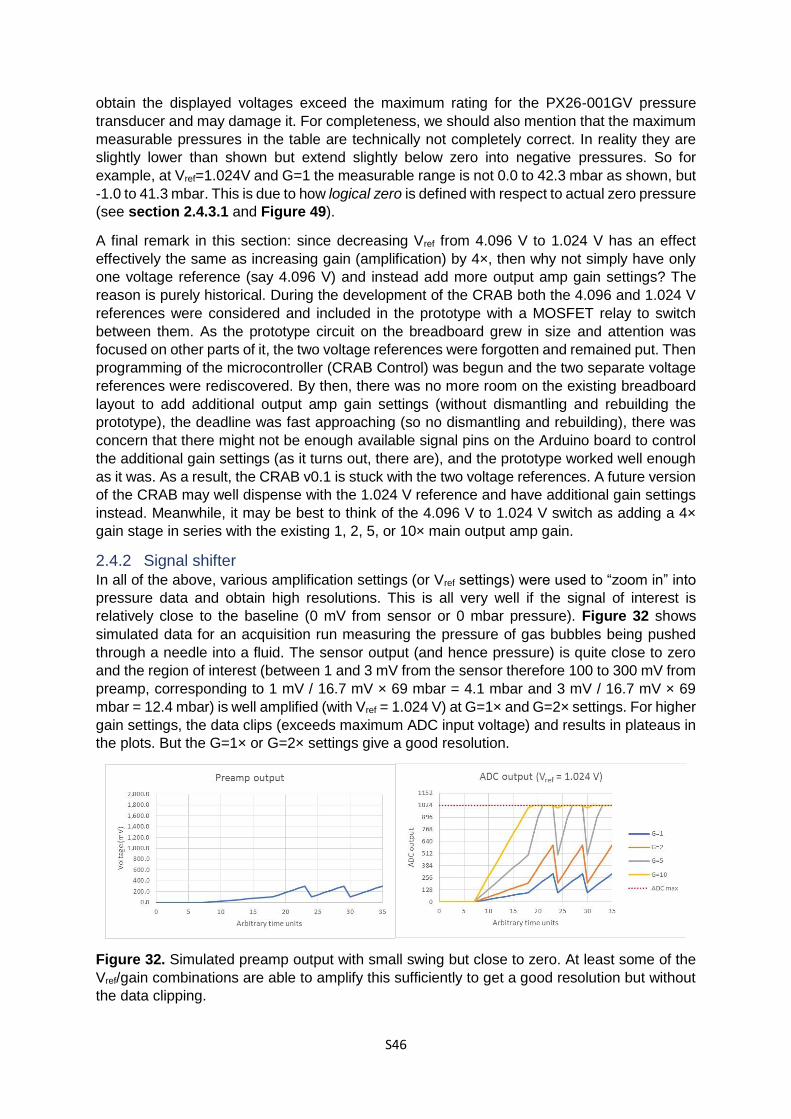
2.4.2 Signal shifter ................................................................................................ S46
2.4.3 The clipper ................................................................................................... S49
3 CRAB Control v0.1 software manual .......................................................................... S51
S22
3.1 Introduction ......................................................................................................... S51
3.2 First-time setup ................................................................................................... S51
3.2.1 Power supply ............................................................................................... S51
3.2.2 Hardware calibration .................................................................................... S51
3.3 Using the CRAB Control v0.1 software ............................................................... S52
3.3.1 Connecting to a computer ............................................................................ S52
3.3.2 Menu structure ............................................................................................. S53
3.3.3 Parameter set structure ............................................................................... S54
3.3.4 Software calibration ..................................................................................... S55
3.3.4.1 Sampling settings ..................................................................................... S55
3.3.4.2 Calibration ................................................................................................ S56
3.3.5 Measuring pressure data ............................................................................. S58
3.3.5.1 Parameter selection ................................................................................. S58
3.3.5.2 Data acquisition ........................................................................................ S60
3.4 Menu options list ................................................................................................. S61
3.4.1 Run .............................................................................................................. S61
3.4.1.1 Run/Sample rate/period............................................................................ S61
3.4.1.2 Run/ADC Vref, amp gain, signal shift ....................................................... S62
3.4.1.3 Run/Run time ........................................................................................... S62
3.4.1.4 Run/Run scouting ..................................................................................... S63
3.4.1.5 Run/Data items ........................................................................................ S65
3.4.1.6 Run/Start run ............................................................................................ S65
3.4.2 Settings ........................................................................................................ S66
3.4.2.1 Settings/Data point stats........................................................................... S66
3.4.2.2 Settings/Signal shifts ................................................................................ S71
3.4.2.3 Settings/Load settings .............................................................................. S72
3.4.2.4 Settings/Save settings .............................................................................. S72
3.4.3 Calibration ................................................................................................... S73
3.4.3.1 Calibration/Zero offset calibration ............................................................. S73
3.4.3.2 Calibration/Span factor calibration ............................................................ S74
3.4.3.3 Calibration/Signal shift digipot calibration ................................................. S75
3.4.3.4 Calibration/Sensor range .......................................................................... S75
3.4.4 Remote operation ........................................................................................ S76
3.4.5 Info .............................................................................................................. S76

S23
1 Hardware manual
1.1 Introduction Cavitational rheology requires the measurement of the internal pressure of minute air bubbles
forming at the tip of a small diameter needle. These pressures are by necessity very small and
a host of external factors could conspire to affect and invalidate pressure readings. The
present experimental setup attempts to mitigate and compensate for some of these factors.
Insertion of a needle into a gel necessarily disrupts the gel at the point of insertion and along
the length of the needle. Any lateral motion of the needle during insertion could conceivably
cause further unnecessary disruption of the gel affecting the measured bubble pressure.
Insertion of the needle into the gel should therefore proceed in a controlled and repeatable
fashion.
Insertion depth is another parameter with possible consequences for the measured pressure.
When bubble pressures were measured in water, it was found that the effect of hydrostatic
pressure (pressure caused by depth of immersion) was easily detected for immersion depth
differences of fractions of a millimetre and with excellent reproducibility (relative standard
deviation < 0.2%) and linearity (R2 > 0.99). Extrapolation of the pressure curve to 0 mm “depth”
allowed the calculation of the dynamic surface tension of the solvent: it was found that, with
corrections for ambient temperature, our setup could also be used as a maximum bubble
pressure tensiometer. How and whether hydrostatic pressure and dynamic surface tension
would come into play in the case of a gel is unclear and was not explored, but it seems prudent
to control for needle immersion depth.
The need for controlled needle insertion and immersion depth prompted us to use a 3D printer
platform, although any electronically controllable xyz-gantry system would be suitable. In the
following, we describe the use of the RepRap Ormerod 1 and Ormerod 2 3D printers for
controlled needle insertion into gel samples, and the device used to measure the bubble
pressures (the “CRAB”).
1.2 3D printer
1.2.1 General The RepRap range of 3D printers presented a low-cost, DIY entry into 3D printing but required
hands-on electronic and mechanical skills to build and operate. An upshot of this was that they
were highly customisable (RepRap actually encouraged users to modify the printers and share
the results with the community). RepRap have unfortunately ceased trading but their printers
can still occasionally be found on internet auction sites (parts, including the electronics, can
still be obtained from http://www.reprapltd.com/). It is on such an auction site that we picked
up and rebuilt an old Ormerod model 1 printer. Our first cavitational rheology experiments
used an Ormerod 2 printer. This printer was also used in our lab for actual 3D printing and had
to be modified every time cavitational rheology experiments were to be carried out. The
Ormerod model 1 was acquired to be a dedicated machine solely for cavitational rheology,
leaving the Ormerod 2 to do 3D printing. The modifications to the printers apply to both the
Ormerod 1 and 2 models (with some minor differences) and are described below. Figure 1
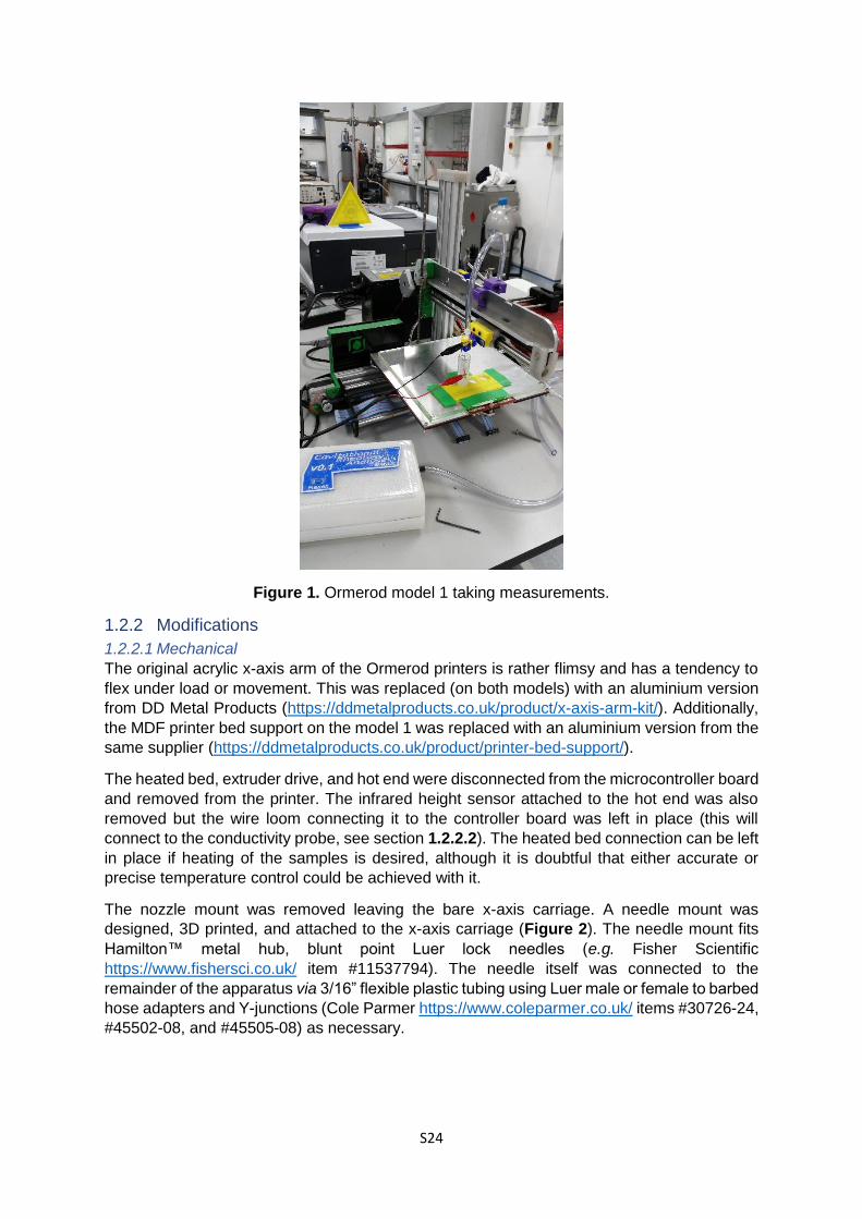
shows our Ormerod model 1 in the process of measuring a sample.
S24
Figure 1. Ormerod model 1 taking measurements.
1.2.2 Modifications
1.2.2.1 Mechanical
The original acrylic x-axis arm of the Ormerod printers is rather flimsy and has a tendency to
flex under load or movement. This was replaced (on both models) with an aluminium version
from DD Metal Products (https://ddmetalproducts.co.uk/product/x-axis-arm-kit/). Additionally,
the MDF printer bed support on the model 1 was replaced with an aluminium version from the
same supplier (https://ddmetalproducts.co.uk/product/printer-bed-support/).
The heated bed, extruder drive, and hot end were disconnected from the microcontroller board
and removed from the printer. The infrared height sensor attached to the hot end was also
removed but the wire loom connecting it to the controller board was left in place (this will
connect to the conductivity probe, see section 1.2.2.2). The heated bed connection can be left
in place if heating of the samples is desired, although it is doubtful that either accurate or
precise temperature control could be achieved with it.
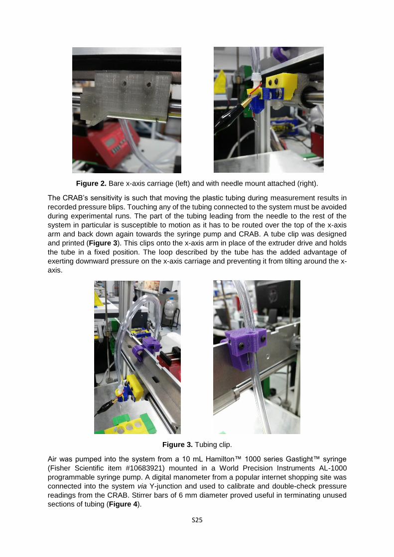
The nozzle mount was removed leaving the bare x-axis carriage. A needle mount was
designed, 3D printed, and attached to the x-axis carriage (Figure 2). The needle mount fits
Hamilton™ metal hub, blunt point Luer lock needles (e.g. Fisher Scientific
https://www.fishersci.co.uk/ item #11537794). The needle itself was connected to the
remainder of the apparatus via 3/16” flexible plastic tubing using Luer male or female to barbed
hose adapters and Y-junctions (Cole Parmer https://www.coleparmer.co.uk/ items #30726-24,
#45502-08, and #45505-08) as necessary.
S25
Figure 2. Bare x-axis carriage (left) and with needle mount attached (right).
The CRAB’s sensitivity is such that moving the plastic tubing during measurement results in
recorded pressure blips. Touching any of the tubing connected to the system must be avoided
during experimental runs. The part of the tubing leading from the needle to the rest of the
system in particular is susceptible to motion as it has to be routed over the top of the x-axis
arm and back down again towards the syringe pump and CRAB. A tube clip was designed
and printed (Figure 3). This clips onto the x-axis arm in place of the extruder drive and holds
the tube in a fixed position. The loop described by the tube has the added advantage of
exerting downward pressure on the x-axis carriage and preventing it from tilting around the x-
axis.
Figure 3. Tubing clip.
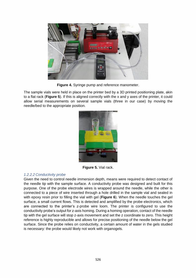
Air was pumped into the system from a 10 mL Hamilton™ 1000 series Gastight™ syringe
(Fisher Scientific item #10683921) mounted in a World Precision Instruments AL-1000
programmable syringe pump. A digital manometer from a popular internet shopping site was
connected into the system via Y-junction and used to calibrate and double-check pressure
readings from the CRAB. Stirrer bars of 6 mm diameter proved useful in terminating unused
sections of tubing (Figure 4).
S26
Figure 4. Syringe pump and reference manometer.
The sample vials were held in place on the printer bed by a 3D printed positioning plate, akin
to a flat rack (Figure 5). If this is aligned correctly with the x and y axes of the printer, it could
allow serial measurements on several sample vials (three in our case) by moving the
needle/bed to the appropriate position.
Figure 5. Vial rack.
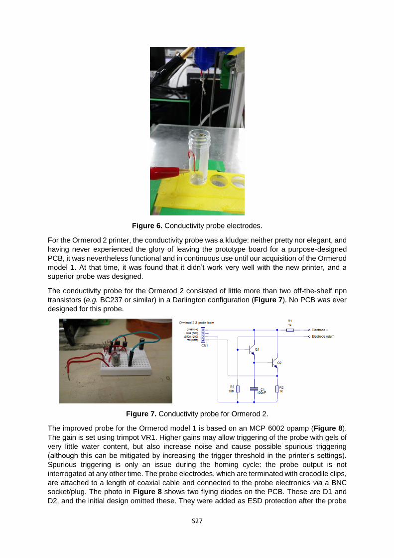
1.2.2.2 Conductivity probe
Given the need to control needle immersion depth, means were required to detect contact of
the needle tip with the sample surface. A conductivity probe was designed and built for this
purpose. One of the probe electrode wires is wrapped around the needle, while the other is
connected to a piece of wire inserted through a hole drilled in the sample vial and sealed in
with epoxy resin prior to filling the vial with gel (Figure 6). When the needle touches the gel
surface, a small current flows. This is detected and amplified by the probe electronics, which
are connected to the printer’s z-probe wire loom. The printer is configured to use the
conductivity probe’s output for z-axis homing. During a homing operation, contact of the needle
tip with the gel surface will stop z-axis movement and set the z coordinate to zero. This height
reference is highly reproducible and allows for precise positioning of the needle below the gel
surface. Since the probe relies on conductivity, a certain amount of water in the gels studied
is necessary: the probe would likely not work with organogels.
S27
Figure 6. Conductivity probe electrodes.
For the Ormerod 2 printer, the conductivity probe was a kludge: neither pretty nor elegant, and
having never experienced the glory of leaving the prototype board for a purpose-designed
PCB, it was nevertheless functional and in continuous use until our acquisition of the Ormerod
model 1. At that time, it was found that it didn’t work very well with the new printer, and a
superior probe was designed.
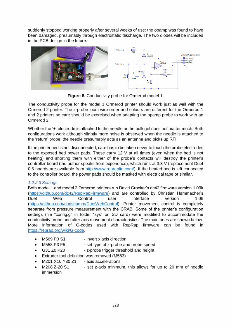
The conductivity probe for the Ormerod 2 consisted of little more than two off-the-shelf npn
transistors (e.g. BC237 or similar) in a Darlington configuration (Figure 7). No PCB was ever
designed for this probe.
Figure 7. Conductivity probe for Ormerod 2.
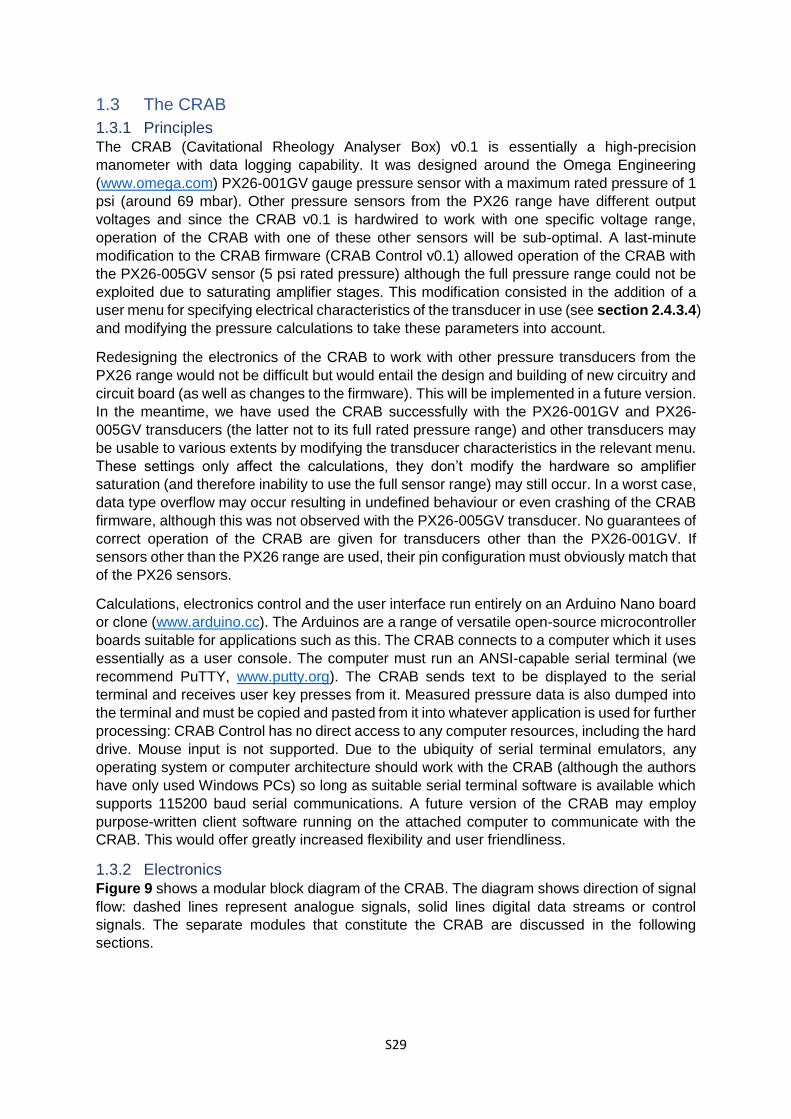
The improved probe for the Ormerod model 1 is based on an MCP 6002 opamp (Figure 8).
The gain is set using trimpot VR1. Higher gains may allow triggering of the probe with gels of
very little water content, but also increase noise and cause possible spurious triggering
(although this can be mitigated by increasing the trigger threshold in the printer’s settings).
Spurious triggering is only an issue during the homing cycle: the probe output is not
interrogated at any other time. The probe electrodes, which are terminated with crocodile clips,
are attached to a length of coaxial cable and connected to the probe electronics via a BNC
socket/plug. The photo in Figure 8 shows two flying diodes on the PCB. These are D1 and
D2, and the initial design omitted these. They were added as ESD protection after the probe
S28
suddenly stopped working properly after several weeks of use: the opamp was found to have
been damaged, presumably through electrostatic discharge. The two diodes will be included
in the PCB design in the future.
Figure 8. Conductivity probe for Ormerod model 1.
The conductivity probe for the model 1 Ormerod printer should work just as well with the
Ormerod 2 printer. The z-probe loom wire order and colours are different for the Ormerod 1
and 2 printers so care should be exercised when adapting the opamp probe to work with an
Ormerod 2.
Whether the ‘+’ electrode is attached to the needle or the bulk gel does not matter much. Both
configurations work although slightly more noise is observed when the needle is attached to
the ‘return’ probe: the needle presumably acts as an antenna and picks up RFI.
If the printer bed is not disconnected, care has to be taken never to touch the probe electrodes
to the exposed bed power pads. These carry 12 V at all times (even when the bed is not
heating) and shorting them with either of the probe’s contacts will destroy the printer’s
controller board (the author speaks from experience), which runs at 3.3 V (replacement Duet
0.6 boards are available from http://www.reprapltd.com/). If the heated bed is left connected
to the controller board, the power pads should be masked with electrical tape or similar.
1.2.2.3 Settings
Both model 1 and model 2 Ormerod printers run David Crocker’s dc42 firmware version 1.09k
(https://github.com/dc42/RepRapFirmware) and are controlled by Christian Hammacher’s
Duet Web Control user interface version 1.06
(https://github.com/chrishamm/DuetWebControl). Printer movement control is completely
separate from pressure measurement with the CRAB. Some of the printer’s configuration
settings (file “config.g” in folder “sys” on SD card) were modified to accommodate the
conductivity probe and alter axis movement characteristics. The main ones are shown below.
More information of G-codes used with RepRap firmware can be found in
https://reprap.org/wiki/G-code.
M569 P0 S1 - invert x axis direction
M558 P3 F5 - set type of z-probe and probe speed
G31 Z0 P20 - z-probe trigger threshold and height
Extruder tool definition was removed (M563)
M201 X10 Y30 Z1 - axis accelerations
M208 Z-20 S1 - set z-axis minimum, this allows for up to 20 mm of needle
immersion
S29
1.3 The CRAB
1.3.1 Principles The CRAB (Cavitational Rheology Analyser Box) v0.1 is essentially a high-precision
manometer with data logging capability. It was designed around the Omega Engineering
(www.omega.com) PX26-001GV gauge pressure sensor with a maximum rated pressure of 1
psi (around 69 mbar). Other pressure sensors from the PX26 range have different output
voltages and since the CRAB v0.1 is hardwired to work with one specific voltage range,
operation of the CRAB with one of these other sensors will be sub-optimal. A last-minute
modification to the CRAB firmware (CRAB Control v0.1) allowed operation of the CRAB with
the PX26-005GV sensor (5 psi rated pressure) although the full pressure range could not be
exploited due to saturating amplifier stages. This modification consisted in the addition of a
user menu for specifying electrical characteristics of the transducer in use (see section 2.4.3.4)
and modifying the pressure calculations to take these parameters into account.
Redesigning the electronics of the CRAB to work with other pressure transducers from the
PX26 range would not be difficult but would entail the design and building of new circuitry and
circuit board (as well as changes to the firmware). This will be implemented in a future version.
In the meantime, we have used the CRAB successfully with the PX26-001GV and PX26-
005GV transducers (the latter not to its full rated pressure range) and other transducers may
be usable to various extents by modifying the transducer characteristics in the relevant menu.
These settings only affect the calculations, they don’t modify the hardware so amplifier
saturation (and therefore inability to use the full sensor range) may still occur. In a worst case,
data type overflow may occur resulting in undefined behaviour or even crashing of the CRAB
firmware, although this was not observed with the PX26-005GV transducer. No guarantees of
correct operation of the CRAB are given for transducers other than the PX26-001GV. If
sensors other than the PX26 range are used, their pin configuration must obviously match that
of the PX26 sensors.
Calculations, electronics control and the user interface run entirely on an Arduino Nano board
or clone (www.arduino.cc). The Arduinos are a range of versatile open-source microcontroller
boards suitable for applications such as this. The CRAB connects to a computer which it uses
essentially as a user console. The computer must run an ANSI-capable serial terminal (we
recommend PuTTY, www.putty.org). The CRAB sends text to be displayed to the serial
terminal and receives user key presses from it. Measured pressure data is also dumped into
the terminal and must be copied and pasted from it into whatever application is used for further
processing: CRAB Control has no direct access to any computer resources, including the hard
drive. Mouse input is not supported. Due to the ubiquity of serial terminal emulators, any
operating system or computer architecture should work with the CRAB (although the authors
have only used Windows PCs) so long as suitable serial terminal software is available which
supports 115200 baud serial communications. A future version of the CRAB may employ
purpose-written client software running on the attached computer to communicate with the
CRAB. This would offer greatly increased flexibility and user friendliness.
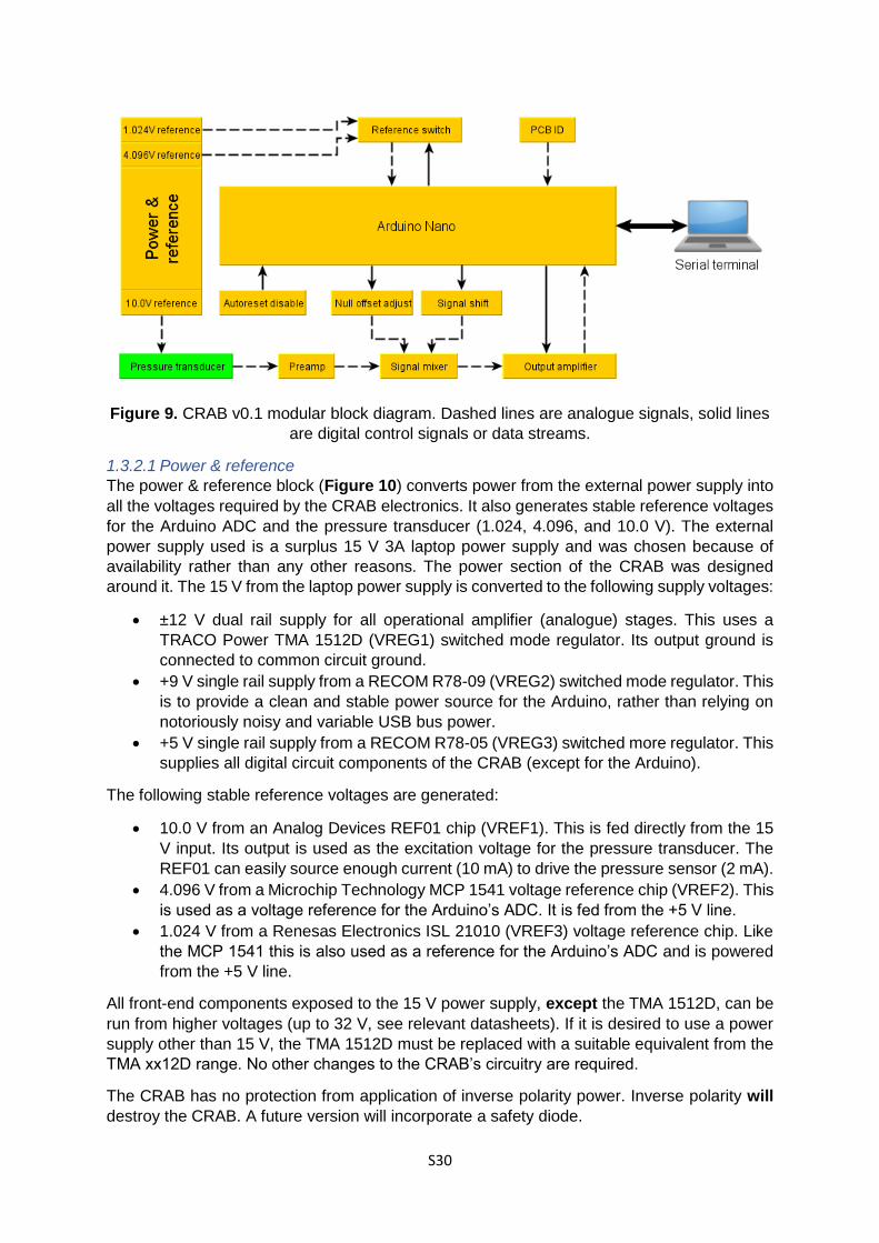
1.3.2 Electronics Figure 9 shows a modular block diagram of the CRAB. The diagram shows direction of signal
flow: dashed lines represent analogue signals, solid lines digital data streams or control
signals. The separate modules that constitute the CRAB are discussed in the following
sections.
S30
Figure 9. CRAB v0.1 modular block diagram. Dashed lines are analogue signals, solid lines
are digital control signals or data streams.
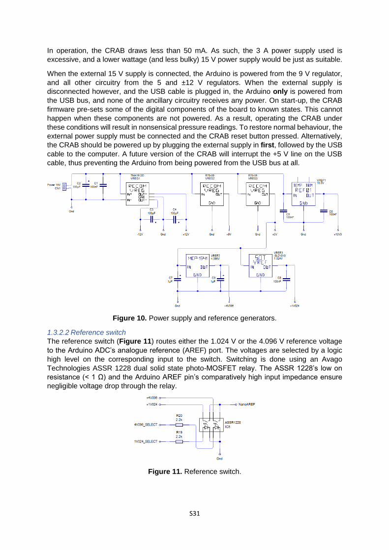
1.3.2.1 Power & reference
The power & reference block (Figure 10) converts power from the external power supply into
all the voltages required by the CRAB electronics. It also generates stable reference voltages
for the Arduino ADC and the pressure transducer (1.024, 4.096, and 10.0 V). The external
power supply used is a surplus 15 V 3A laptop power supply and was chosen because of
availability rather than any other reasons. The power section of the CRAB was designed
around it. The 15 V from the laptop power supply is converted to the following supply voltages:
±12 V dual rail supply for all operational amplifier (analogue) stages. This uses a
TRACO Power TMA 1512D (VREG1) switched mode regulator. Its output ground is
connected to common circuit ground.
+9 V single rail supply from a RECOM R78-09 (VREG2) switched mode regulator. This
is to provide a clean and stable power source for the Arduino, rather than relying on
notoriously noisy and variable USB bus power.
+5 V single rail supply from a RECOM R78-05 (VREG3) switched more regulator. This
supplies all digital circuit components of the CRAB (except for the Arduino).
The following stable reference voltages are generated:
10.0 V from an Analog Devices REF01 chip (VREF1). This is fed directly from the 15
V input. Its output is used as the excitation voltage for the pressure transducer. The
REF01 can easily source enough current (10 mA) to drive the pressure sensor (2 mA).
4.096 V from a Microchip Technology MCP 1541 voltage reference chip (VREF2). This
is used as a voltage reference for the Arduino’s ADC. It is fed from the +5 V line.
1.024 V from a Renesas Electronics ISL 21010 (VREF3) voltage reference chip. Like
the MCP 1541 this is also used as a reference for the Arduino’s ADC and is powered
from the +5 V line.
All front-end components exposed to the 15 V power supply, except the TMA 1512D, can be
run from higher voltages (up to 32 V, see relevant datasheets). If it is desired to use a power
supply other than 15 V, the TMA 1512D must be replaced with a suitable equivalent from the
TMA xx12D range. No other changes to the CRAB’s circuitry are required.
The CRAB has no protection from application of inverse polarity power. Inverse polarity will
destroy the CRAB. A future version will incorporate a safety diode.
S31
In operation, the CRAB draws less than 50 mA. As such, the 3 A power supply used is
excessive, and a lower wattage (and less bulky) 15 V power supply would be just as suitable.
When the external 15 V supply is connected, the Arduino is powered from the 9 V regulator,
and all other circuitry from the 5 and ±12 V regulators. When the external supply is
disconnected however, and the USB cable is plugged in, the Arduino only is powered from
the USB bus, and none of the ancillary circuitry receives any power. On start-up, the CRAB
firmware pre-sets some of the digital components of the board to known states. This cannot
happen when these components are not powered. As a result, operating the CRAB under
these conditions will result in nonsensical pressure readings. To restore normal behaviour, the
external power supply must be connected and the CRAB reset button pressed. Alternatively,
the CRAB should be powered up by plugging the external supply in first, followed by the USB
cable to the computer. A future version of the CRAB will interrupt the +5 V line on the USB
cable, thus preventing the Arduino from being powered from the USB bus at all.
Figure 10. Power supply and reference generators.
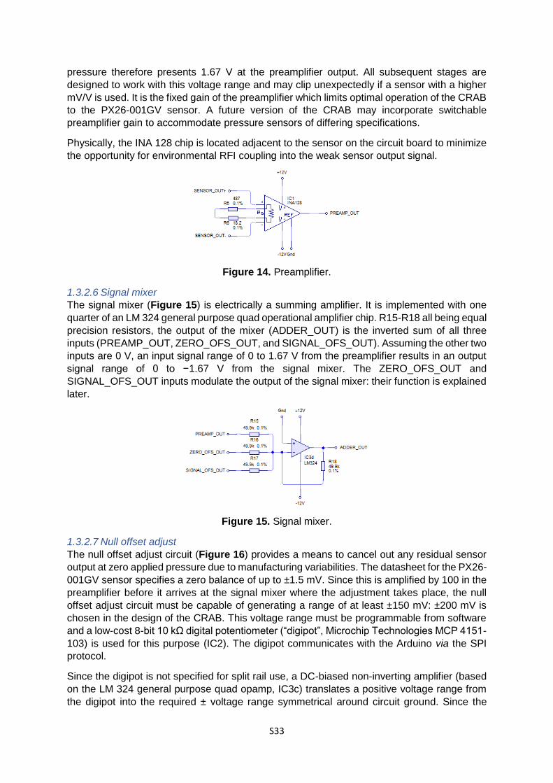
1.3.2.2 Reference switch
The reference switch (Figure 11) routes either the 1.024 V or the 4.096 V reference voltage
to the Arduino ADC’s analogue reference (AREF) port. The voltages are selected by a logic
high level on the corresponding input to the switch. Switching is done using an Avago
Technologies ASSR 1228 dual solid state photo-MOSFET relay. The ASSR 1228’s low on
resistance (< 1 Ω) and the Arduino AREF pin’s comparatively high input impedance ensure
negligible voltage drop through the relay.
Figure 11. Reference switch.

S32
1.3.2.3 PCB ID
The PCB ID circuit is a means by which firmware running on the Arduino can detect what
version of CRAB hardware it is running on and issue a warning if it is not compatible with that
hardware. The PCB ID circuit consists of two voltage dividers between the Arduino’s +5 V pin
and the ground rail with resistance values chosen as shown in Figure 12. The resistors are of
high precision (±0.1 %) type and with the values chosen deliver voltages of 1.67 V (PCB_ID1)
and 2.50 V (PCB_ID2) to analogue input ports on the Arduino. These voltages are
characteristic for this (v0.1) hardware version. Any future revisions of the CRAB hardware
must choose different resistor combinations to identify the board version to the firmware.
Figure 12. PCB ID.
1.3.2.4 Autoreset disable
Establishing a serial connection over USB resets the Arduino and restarts the firmware. This
may be undesirable in some circumstances, e.g. when serial communication is lost for any
reason while modified CRAB settings have not been saved to EEPROM yet. In this case,
communications can be re-established without resetting the CRAB and allowing saving of the
modified settings. To disable autoreset, pins J1 are shorted with a jumper (Figure 13).
Removing the jumper restores autoreset behaviour.
Prior to using the CRAB, the firmware must be uploaded to the Arduino. Disabling autoreset
interferes with this process. To upload code from the Arduino IDE with autoreset disabled, the
reset button on the Arduino is pressed and held, and the compilation and upload process is
started by pressing the upload button in the Arduino IDE, while closely monitoring the RX LED
on the Arduino. The LED will flash briefly when the upload is about to begin. At this point the
reset button is released immediately and the upload should proceed. Some trial and error may
be required to get the timing right. Alternatively, autoreset can be enabled (by removing jumper
J1) for the duration of the firmware upload.
Figure 13. Autoreset disable.
1.3.2.5 Preamplifier
The CRAB was designed around the PX26-001GV Wheatstone bridge-type pressure
transducer with an output of 1.67 mV/V at its rated pressure (1 psi), or 16.7 mV with 10.0 V
excitation. The differential floating output of the transducer is fed into a INA 128 single chip
instrumentation amplifier (Figure 14), with R5 and R6 precision resistors in series setting a
fixed gain of 100 in hardware (see INA 128 datasheet). The PX26-001GV sensor at rated
S33
pressure therefore presents 1.67 V at the preamplifier output. All subsequent stages are
designed to work with this voltage range and may clip unexpectedly if a sensor with a higher
mV/V is used. It is the fixed gain of the preamplifier which limits optimal operation of the CRAB
to the PX26-001GV sensor. A future version of the CRAB may incorporate switchable
preamplifier gain to accommodate pressure sensors of differing specifications.
Physically, the INA 128 chip is located adjacent to the sensor on the circuit board to minimize
the opportunity for environmental RFI coupling into the weak sensor output signal.
Figure 14. Preamplifier.
1.3.2.6 Signal mixer
The signal mixer (Figure 15) is electrically a summing amplifier. It is implemented with one
quarter of an LM 324 general purpose quad operational amplifier chip. R15-R18 all being equal
precision resistors, the output of the mixer (ADDER_OUT) is the inverted sum of all three
inputs (PREAMP_OUT, ZERO_OFS_OUT, and SIGNAL_OFS_OUT). Assuming the other two
inputs are 0 V, an input signal range of 0 to 1.67 V from the preamplifier results in an output
signal range of 0 to −1.67 V from the signal mixer. The ZERO_OFS_OUT and
SIGNAL_OFS_OUT inputs modulate the output of the signal mixer: their function is explained
later.
Figure 15. Signal mixer.
1.3.2.7 Null offset adjust
The null offset adjust circuit (Figure 16) provides a means to cancel out any residual sensor
output at zero applied pressure due to manufacturing variabilities. The datasheet for the PX26-
001GV sensor specifies a zero balance of up to ±1.5 mV. Since this is amplified by 100 in the
preamplifier before it arrives at the signal mixer where the adjustment takes place, the null
offset adjust circuit must be capable of generating a range of at least ±150 mV: ±200 mV is
chosen in the design of the CRAB. This voltage range must be programmable from software
and a low-cost 8-bit 10 kΩ digital potentiometer (“digipot”, Microchip Technologies MCP 4151-
103) is used for this purpose (IC2). The digipot communicates with the Arduino via the SPI
protocol.
Since the digipot is not specified for split rail use, a DC-biased non-inverting amplifier (based
on the LM 324 general purpose quad opamp, IC3c) translates a positive voltage range from
the digipot into the required ± voltage range symmetrical around circuit ground. Since the

S34
required output swing is 400 mV (±200 mV) and non-inverting amplifiers cannot have unit gain,
an integer gain of 2 is chosen with R8 = R9 (𝐺 = 1 +𝑅8
𝑅9= 2). The required input swing into the
operational amplifier is therefore 0 to +200 mV for a desired output swing of −200 to +200 mV.
The equation describing this amplifier topology (𝑉𝑜𝑢𝑡 = 2𝑉𝑖𝑛 + (1 − 𝐺)𝑉𝑏𝑖𝑎𝑠) gives the required
bias voltage as 200 mV. This is derived from a voltage divider (R10 and VR2) between the 5
V power rails and fine-tuned using multi-turn potentiometer VR2 (see section 1.3.3).
The input voltage swing (0 to 200 mV) is derived from the digipot (IC2) conFigured as a voltage
divider providing a voltage range of approximately 0 to +5 V in 256 (8 bit) steps. This is fed
into a further voltage divider (R7 and VR1) generating a much reduced voltage swing. VR1 is
used to fine-tune this to the required 0 to 200 mV. This is done so that approximately 100 mV
is measured at TP1. The reason that this is set to 100 mV and not 200 mV is that, when first
powered up, the MCP 4151-103 digipot defaults to its midpoint setting, which translates to the
midpoint of the 0 to 200 mV range, i.e. 100 mV. Correct adjustment of VR1 relies on this fact
and this must therefore be carried out before the setting of the IC2 digipot is changed in any
way by software (see section 1.3.3).
In operation, the null offset adjust signal is combined in the signal mixer with the output of the
preamplifier to bring their sum as close as possible to 0 when no pressure is applied to the
sensor.
Figure 16. Null offset adjust.
1.3.2.8 Signal shift
The signal shifter was added to the CRAB mainly because of the limited (10 bit) resolution of
the Arduino’s ADC. Without the signal shifter, the choices would have been (depending on
amplifier settings) either full sensor pressure range measurement with low resolution, or
measurement of a smaller window of the full pressure range (beginning at zero) with higher
resolution. While the signal shifter cannot improve hardware resolution, it allows a narrow but
high resolution “zoom” window to be moved up through the entire measurable pressure range.
If for instance an event of interest occurs near the top of the pressure range and high resolution
is required, amplifier and sampling settings are chosen to shrink the measurable pressure
window (and with this the smallest measurable pressure difference), and the signal shifter is
then used to shift this window up towards the pressure range of interest. Pressures below that
window will not be measured (they will “clip”, see section 2.3.1) but the pressures inside the
window can be measured with much greater precision. The signal shifter is an unsatisfactory
solution to a problem caused by the limited resolution of the Arduino’s ADC. It would not have
been necessary had a superior, external ADC chip been used in the first place, and this will
be implemented in a future version of the CRAB.
The signal shifter (Figure 17) works in a manner similar to the null offset adjust circuit, by
injecting a voltage offset into the signal mixer to be combined with the signal from the sensor
(and any null offset compensation). Unlike the null offset voltage generator, the signal required

S35
does not need to extend into both the positive and negative voltages. This makes the
electronics simpler since only a negative signal is required (mixing the preamp signal with a
negative voltage effectively shifts the preamp output closer to zero, but since the measured
pressure has not changed, the measurable pressure “window” has effectively shifted upwards).
Digital control is again provided by a MCP 4151-103 digipot (IC4) which drives an inverting
unity gain buffer.
The digipot output (ca. 0 to +5 V) is converted to a range 0 to +2 V by voltage divider R11 and
R12. This should in theory have been 3.4 V, but mismatched impedances between this and
the subsequent buffer stage drive this down to closer to 2 volts. This will be fixed in a future
version of the CRAB. The inverting unity gain buffer is based on the LM 324 general purpose
opamp chip (IC3b), conFigured as a unity gain (𝐺 =𝑅14
𝑅13= 1) inverting amplifier. 0 to +2 V is
thus translated into 0 to −2 V at the SIGNAL_OFS_OUT output. This is fed into the signal
mixer and the possible output range of the mixer now changes from 0 to −1.67 V to +2 to
−1.67 V (the signal mixer is inverting). The shift achievable by the signal shifter is sufficient to
move the pre-amplified sensor output over its entire rated pressure range out of the standard
sampling window of the Arduino and thus position the sampling window at the very top of the
sensor pressure range. This allows high resolution measurements at the very top of and above
the rated sensor pressure range (see section 2.4.2).
Figure 17. Signal shifter.
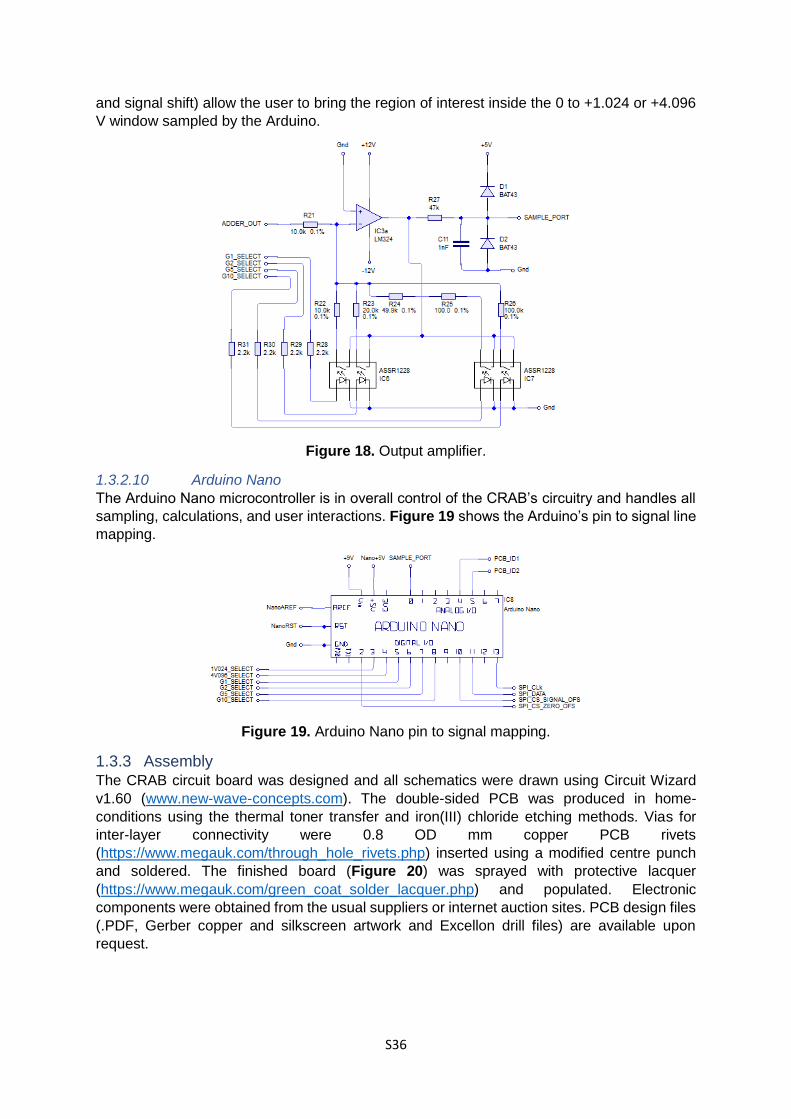
1.3.2.9 Output amplifier
The final stage amplifier (Figure 18) takes the output of the signal mixer (possible range +2
to −1.67 V), inverts it back into phase with the original pressure sensor output (the signal mixer
was inverting), and applies a final amplification factor of 1 (no amplification), 2, 5, or 10. The
final amplification factor is selected by applying a logic high control signal to one of the
G1_SELECT, G2_SELECT, G5_SELECT, or G10_SELECT inputs. These drive ASSR 1228
solid state relays to switch the gain resistor network. The gain network itself is built from
precision resistors (R22-R26). The small on resistance of the solid state switches is negligible
compared to the resistance values in the network. The amplifier itself is based on the
remaining unused opamp (IC3a) of the LM 324 chip.
The output of the amplifier is fed through a low-pass filter (R27 and C11) with cutoff frequency
ca. 3 kHz, and finally through a voltage clipper (Schottky diodes D1 and D2), before being fed
into the Arduino’s ADC input. The clipper limits the amplifier output to a 0 to +5 V swing safe
for the Arduino.
At the highest final amplification factor of 10, the theoretical output swing of the output amplifier
could be −20 to +16.7 V. In practice this is limited by the ±12 V power rail and the fact that the
LM 324 is incapable of rail-to-rail output, but a Figure of around ±10 V seems plausible.
Pressure data of interest could be anywhere in this window and the CRAB’s settings (Vref, gain,
S36
and signal shift) allow the user to bring the region of interest inside the 0 to +1.024 or +4.096
V window sampled by the Arduino.
Figure 18. Output amplifier.
1.3.2.10 Arduino Nano
The Arduino Nano microcontroller is in overall control of the CRAB’s circuitry and handles all
sampling, calculations, and user interactions. Figure 19 shows the Arduino’s pin to signal line
mapping.
Figure 19. Arduino Nano pin to signal mapping.
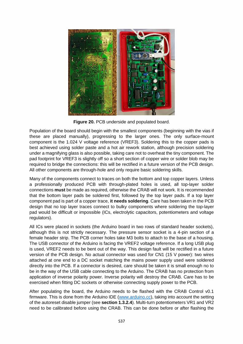
1.3.3 Assembly The CRAB circuit board was designed and all schematics were drawn using Circuit Wizard
v1.60 (www.new-wave-concepts.com). The double-sided PCB was produced in home-
conditions using the thermal toner transfer and iron(III) chloride etching methods. Vias for
inter-layer connectivity were 0.8 OD mm copper PCB rivets
(https://www.megauk.com/through_hole_rivets.php) inserted using a modified centre punch
and soldered. The finished board (Figure 20) was sprayed with protective lacquer
(https://www.megauk.com/green_coat_solder_lacquer.php) and populated. Electronic
components were obtained from the usual suppliers or internet auction sites. PCB design files
(.PDF, Gerber copper and silkscreen artwork and Excellon drill files) are available upon
request.
S37
Figure 20. PCB underside and populated board.
Population of the board should begin with the smallest components (beginning with the vias if
these are placed manually), progressing to the larger ones. The only surface-mount
component is the 1.024 V voltage reference (VREF3). Soldering this to the copper pads is
best achieved using solder paste and a hot air rework station, although precision soldering
under a magnifying glass is also possible, taking care not to overheat the tiny component. The
pad footprint for VREF3 is slightly off so a short section of copper wire or solder blob may be
required to bridge the connections: this will be rectified in a future version of the PCB design.
All other components are through-hole and only require basic soldering skills.
Many of the components connect to traces on both the bottom and top copper layers. Unless
a professionally produced PCB with through-plated holes is used, all top-layer solder
connections must be made as required, otherwise the CRAB will not work. It is recommended
that the bottom layer pads be soldered first, followed by the top layer pads. If a top layer
component pad is part of a copper trace, it needs soldering. Care has been taken in the PCB
design that no top layer traces connect to bulky components where soldering the top-layer
pad would be difficult or impossible (ICs, electrolytic capacitors, potentiometers and voltage
regulators).
All ICs were placed in sockets (the Arduino board in two rows of standard header sockets),
although this is not strictly necessary. The pressure sensor socket is a 4-pin section of a
female header strip. The PCB corner holes take M3 bolts to attach to the base of a housing.
The USB connector of the Arduino is facing the VREF2 voltage reference. If a long USB plug
is used, VREF2 needs to be bent out of the way. This design fault will be rectified in a future
version of the PCB design. No actual connector was used for CN1 (15 V power): two wires
attached at one end to a DC socket matching the mains power supply used were soldered
directly into the PCB. If a connector is desired, care should be taken it is small enough no to
be in the way of the USB cable connecting to the Arduino. The CRAB has no protection from
application of inverse polarity power. Inverse polarity will destroy the CRAB. Care has to be
exercised when fitting DC sockets or otherwise connecting supply power to the PCB.
After populating the board, the Arduino needs to be flashed with the CRAB Control v0.1
firmware. This is done from the Arduino IDE (www.arduino.cc), taking into account the setting
of the autoreset disable jumper (see section 1.3.2.4). Multi-turn potentiometers VR1 and VR2
need to be calibrated before using the CRAB. This can be done before or after flashing the
S38
firmware, but before interacting with the CRAB’s user interface in any way (see section
1.3.2.7).
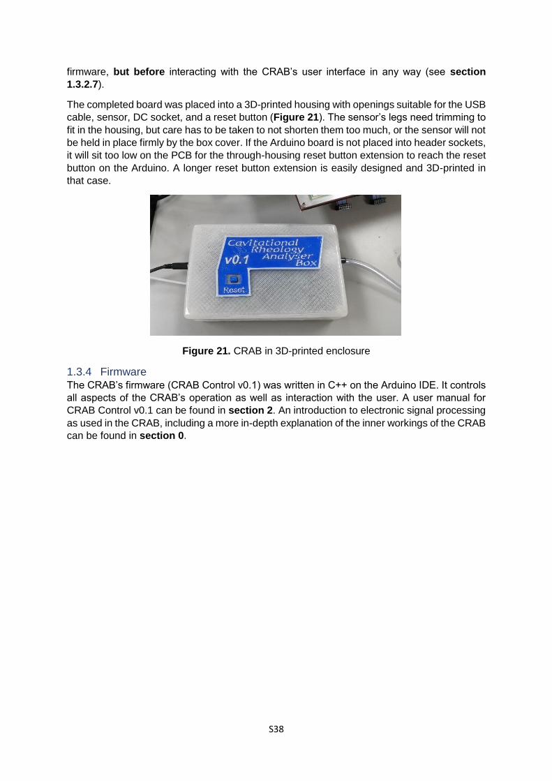
The completed board was placed into a 3D-printed housing with openings suitable for the USB
cable, sensor, DC socket, and a reset button (Figure 21). The sensor’s legs need trimming to
fit in the housing, but care has to be taken to not shorten them too much, or the sensor will not
be held in place firmly by the box cover. If the Arduino board is not placed into header sockets,
it will sit too low on the PCB for the through-housing reset button extension to reach the reset
button on the Arduino. A longer reset button extension is easily designed and 3D-printed in
that case.
Figure 21. CRAB in 3D-printed enclosure
1.3.4 Firmware The CRAB’s firmware (CRAB Control v0.1) was written in C++ on the Arduino IDE. It controls
all aspects of the CRAB’s operation as well as interaction with the user. A user manual for
CRAB Control v0.1 can be found in section 2. An introduction to electronic signal processing
as used in the CRAB, including a more in-depth explanation of the inner workings of the CRAB
can be found in section 0.
S39
2 Operating principles
2.1 Introduction This section is intended for the reader unfamiliar with electronics and electronic signal
processing. It describes the principles that underlie the working of the CRAB v0.1. While a
detailed understanding of the electronics is not required for the successful use of the CRAB,
some basic understanding will clarify the various options available in CRAB Control (the
software running on the CRAB) and lead to their more effective use. A more detailed
description of the electronics is found in section 1.3.2. The reader familiar with electronics
and signal processing basics may skip ahead to section 2, the CRAB Control user manual.
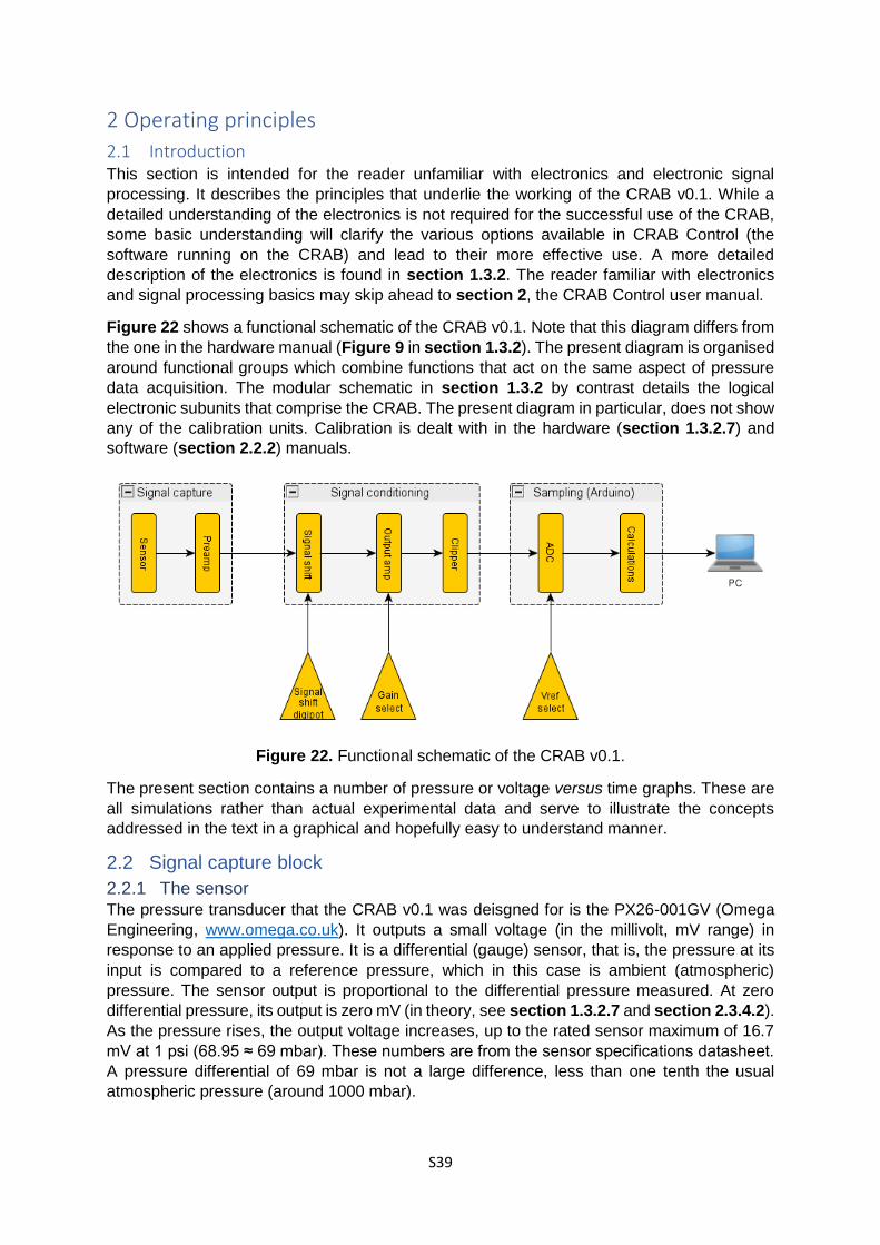
Figure 22 shows a functional schematic of the CRAB v0.1. Note that this diagram differs from
the one in the hardware manual (Figure 9 in section 1.3.2). The present diagram is organised
around functional groups which combine functions that act on the same aspect of pressure
data acquisition. The modular schematic in section 1.3.2 by contrast details the logical
electronic subunits that comprise the CRAB. The present diagram in particular, does not show
any of the calibration units. Calibration is dealt with in the hardware (section 1.3.2.7) and
software (section 2.2.2) manuals.
Figure 22. Functional schematic of the CRAB v0.1.
The present section contains a number of pressure or voltage versus time graphs. These are
all simulations rather than actual experimental data and serve to illustrate the concepts
addressed in the text in a graphical and hopefully easy to understand manner.
2.2 Signal capture block
2.2.1 The sensor The pressure transducer that the CRAB v0.1 was deisgned for is the PX26-001GV (Omega
Engineering, www.omega.co.uk). It outputs a small voltage (in the millivolt, mV range) in
response to an applied pressure. It is a differential (gauge) sensor, that is, the pressure at its
input is compared to a reference pressure, which in this case is ambient (atmospheric)
pressure. The sensor output is proportional to the differential pressure measured. At zero
differential pressure, its output is zero mV (in theory, see section 1.3.2.7 and section 2.3.4.2).
As the pressure rises, the output voltage increases, up to the rated sensor maximum of 16.7
mV at 1 psi (68.95 ≈ 69 mbar). These numbers are from the sensor specifications datasheet.
A pressure differential of 69 mbar is not a large difference, less than one tenth the usual
atmospheric pressure (around 1000 mbar).
S40
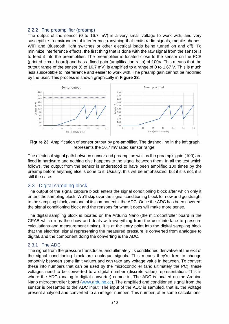
2.2.2 The preamplifier (preamp) The output of the sensor (0 to 16.7 mV) is a very small voltage to work with, and very
susceptible to environmental interference (anything that emits radio signals, mobile phones,
WiFi and Bluetooth, light switches or other electrical loads being turned on and off). To
minimize interference effects, the first thing that is done with the raw signal from the sensor is
to feed it into the preamplifier. The preamplifier is located close to the sensor on the PCB
(printed circuit board) and has a fixed gain (amplification ratio) of 100×. This means that the
output range of the sensor (0 to 16.7 mV) is amplified to a range of 0 to 1.67 V. This is much
less susceptible to interference and easier to work with. The preamp gain cannot be modified
by the user. This process is shown graphically in Figure 23.
Figure 23. Amplification of sensor output by pre-amplifier. The dashed line in the left graph
represents the 16.7 mV rated sensor range.
The electrical signal path between sensor and preamp, as well as the preamp’s gain (100) are
fixed in hardware and nothing else happens to the signal between them. In all the text which
follows, the output from the sensor is understood to have been amplified 100 times by the
preamp before anything else is done to it. Usually, this will be emphasized, but if it is not, it is
still the case.
2.3 Digital sampling block The output of the signal capture block enters the signal conditioning block after which only it
enters the sampling block. We’ll skip over the signal conditioning block for now and go straight
to the sampling block, and one of its components, the ADC. Once the ADC has been covered,
the signal conditioning block and the reasons for what it does will make more sense.
The digital sampling block is located on the Arduino Nano (the microcontroller board in the
CRAB which runs the show and deals with everything from the user interface to pressure
calculations and measurement timing). It is at the entry point into the digital sampling block
that the electrical signal representing the measured pressure is converted from analogue to
digital, and the component doing the converting is the ADC.
2.3.1 The ADC The signal from the pressure transducer, and ultimately its conditioned derivative at the exit of
the signal conditioning block are analogue signals. This means they’re free to change
smoothly between some limit values and can take any voltage value in between. To convert
these into numbers that can be used by the microcontroller (and ultimately the PC), these
voltages need to be converted to a digital number (discrete value) representation. This is
where the ADC (analog-to-digital converter) comes in. The ADC is located on the Arduino
Nano microcontroller board (www.arduino.cc). The amplified and conditioned signal from the
sensor is presented to the ADC input. The input of the ADC is sampled, that is, the voltage
present analysed and converted to an integer number. This number, after some calculations,

S41
is now available as a pressure reading. The ADC on the Arduino has some limitations which
are important to understand.
First, it has only a 10-bit resolution. This means that the input voltage range which it can
sample is converted to a range of 1024 (210 = 1024) discrete values, from 0 to 1023 (all integer
numbers). For example, if the input range were 0 to 2 V (it isn’t, more on this later), then a
voltage of 1 V at the input would be converted to 512 (midpoint between 0 and 1023) by the
ADC. It also means that the smallest change in voltage which can be detected by the ADC is
2 V / 1024 steps = 0.00195 V/step, or 1.95 mV per step. If we consider our sensor’s pre-
amplified output range of 0 to 1.67 V (16.7 mV × 100) and the corresponding full-scale
pressure of 69 mbar, a step of 1.95 mV corresponds to a pressure difference of 0.00195 V /
1.67 V × 69 mbar ≈ 0.1 mbar. This is not a bad resolution, but keep in mind that this is over
the entire range of the sensor, i.e. 0 to 69 mbar. If the pressure of interest varies between, say,
8.0 and 9.0 mbar, then suddenly 0.1 mbar is only 10 steps and any data plotted from this
would have very obvious coarse steps (Figure 24). This effect is called quantization and is
the result of insufficient resolution for the data range of interest or zooming too deeply into a
section of data. Quantization in picture processing manifests as an effect better known as
“pixellation”.
Figure 24. Effects of quantization due to insufficient resolution.
Figure 25 shows the same plots of pressure variations and corresponding ADC output as
above but shown within the entire pressure ranges of the sensor and ADC window. The
sinusoidal shape is barely recognisable. Only a small fraction of the available sensor range is
used, and this is reflected in the small fraction of the available ADC input window. The
resolution (0.1 mbar) over the entire range (0 to 69 mbar) is good, but is less so when looking
at a fine detail.
Figure 25. Same plots as above but shown within entire pressure range of sensor and ADC
sampling window.
A second limitation of the ADC is its input or sampling window. The ADC input will not accept
just any arbitrary voltage. There must be lower and upper limits otherwise the chip would not
S42
know what voltage to call 0 and what to call 1023. The lower limit is conveniently 0 V. The
upper limit depends on a reference voltage (Vref). The reference voltage is a precisely known
voltage used as an upper reference for analog signal sampling. On the Arduino, the range 0
to Vref is subdivided into 1024 steps (10 bit resolution) and any input into the ADC is mapped
onto one of the 1024 (0 to 1023) possible integer values.
The Arduinos’ default Vref is its own supply voltage. Since Arduino boards are usually powered
via USB, this is about 5 V. USB power however is notoriously unstable and noisy, and
therefore not appropriate to use as a refernce for a high precision application. Instead, the
CRAB uses high-stability voltage references on the main circuit board and feeds the output of
these into the Arduino board to use as Vref.
The CRAB has two selectable reference voltages: 1.024 V and 4.096 V. This is shown in
Figure 22 as the “Vref select” icon. When Vref 4.096 V is active, the range from 0 to 4.096 V
is subdivided into 1024 (10 bit resolution) steps. Each step is therefore 4.096 V / 1024 steps
= 0.004 V/step or 4 mV per step. For our sensor (pre-amplified range 0 to 1.67 V corresponding
to 0 to 69 mbar) 4 mV corresponds to 0.004 V / 1.67 V × 69 mbar = 0.16 mbar and this is the
hardware resolution at this Vref setting.
When Vref 1.024 V is active, the range from 0 to 1.024 V is subdivided into 1024 steps. Each
step is therefore 1.024 V / 1024 steps = 0.001 V/step or 1 mV per step. For our sensor again,
1 mV corresponds to 0.001 V / 1.67 V × 69 mbar = 0.04 mbar. The resolution has increased
by a factor of 4 from the previous 4.096 V setting, but the ADC window has shrunk (from 0 to
4.096 V down to 0 to 1.024 V). The important thing to remember is that decreasing the Vref
voltage increases resolution but decreases the range of input voltages that the ADC can
accept.
Voltages above or below the ADC window (0 to Vref) are clipped. Clipping refers to the cutting
off of a signal above or below a maximum or minimum threshold. Any voltage below 0 V is
translated as 0 by the ADC, and any voltage above Vref is translated as 1023. Clipping is
usually very obvious in plots as it results in unexpected plateaus. It is illustrated in section
2.4.2 about signal shifting.
ADC input voltages much below 0 V or much above 5 V (the Arduino operates at 5 V) can
physically damage the microcontroller board. Such voltages can be generated by the signal
conditioning and amplification circuitry in the CRAB (since it operates on a −12 to +12 V split
rail supply) but are cut off (clipped intentionally) by the clipper (last stage of signal conditioning
section in Figure 22, see also section 2.4.3) before they reach the Arduino and no user
intervention is required to protect the microcontroller board.
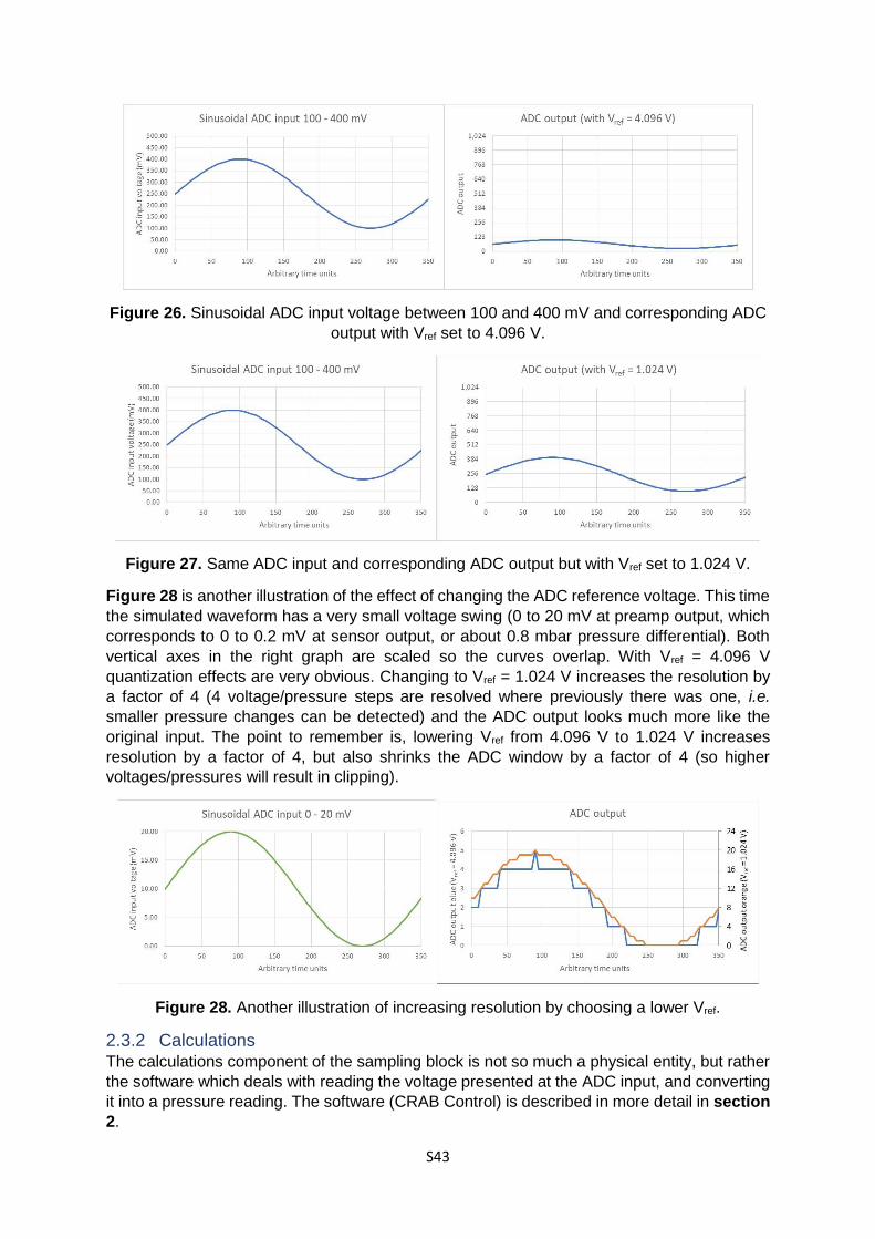
Figures 26 and 27 show the effect of changing Vref from 4.096 V to 1.024 V on the same ADC
input waveform. Remember that this waveform was itself already amplified 100 times by the
preamp, so the original sensor output was 100 smaller. The simulated sinusoidal waveform
below (between 100 and 400 mV) corresponds to an original sensor output between 1 and 4
mV, which itself corresponds to a pressure swing between (according to published sensor
specifications) 1 mV / 16.7 mV × 69 mbar ≈ 4 mbar and 4 mV / 16.7 mV × 69 mbar ≈ 16 mbar.
The increased swing of the ADC output is obvious. With it comes increased resolution.
S43
Figure 26. Sinusoidal ADC input voltage between 100 and 400 mV and corresponding ADC
output with Vref set to 4.096 V.
Figure 27. Same ADC input and corresponding ADC output but with Vref set to 1.024 V.
Figure 28 is another illustration of the effect of changing the ADC reference voltage. This time
the simulated waveform has a very small voltage swing (0 to 20 mV at preamp output, which
corresponds to 0 to 0.2 mV at sensor output, or about 0.8 mbar pressure differential). Both
vertical axes in the right graph are scaled so the curves overlap. With Vref = 4.096 V
quantization effects are very obvious. Changing to Vref = 1.024 V increases the resolution by
a factor of 4 (4 voltage/pressure steps are resolved where previously there was one, i.e.
smaller pressure changes can be detected) and the ADC output looks much more like the
original input. The point to remember is, lowering Vref from 4.096 V to 1.024 V increases
resolution by a factor of 4, but also shrinks the ADC window by a factor of 4 (so higher
voltages/pressures will result in clipping).
Figure 28. Another illustration of increasing resolution by choosing a lower Vref.
2.3.2 Calculations The calculations component of the sampling block is not so much a physical entity, but rather
the software which deals with reading the voltage presented at the ADC input, and converting
it into a pressure reading. The software (CRAB Control) is described in more detail in section
2.

S44
2.4 Signal conditioning block The pre-amplified signal from the pressure transducer is fed into the signal conditioning block.
Here, it is altered in a number of controlled ways dependent on user settings. The first
alteration, and one not shown in Figure 22, is to compensate for transducer zero offset. This
is covered under calibration in section 1.3.2.7 and section 2.3.4.2. Further alterations include
the signal shift utility, and the output amplifier, both covered in the following. The output
amplifier will be discussed first, since understanding its function will help in understanding the
reason for and function of the signal shifter.
2.4.1 Output amplifier The output amplifier does exactly what its name suggests: it further amplifies the conditioned
signal before passing it on to the clipper, and finally the sampling block. In all the previous
discussion an output amp gain of 1 (no amplification) was assumed and there was therefore
no need to mention it: it was as if it didn’t exist. The CRAB has four selectable output amp
gain settings: 1, 2, 5, and 10× (these are represented as the “Gain select” icon in Figure 22).
These take the output of the preamp and amplify it 1, 2, 5, or 10 times. Taking into account
the preamp’s fixed gain of 100, the effective amplification factor between sensor output and
ADC input can therefore be 100, 200, 500, or 1000×.
For example, at the highest gain setting, a sensor voltage swing from 0 to 1 mV is amplified
to 0 to 100 mV by the preamp, which is amplified to 0 to 1000 mV (0 to 1 V) by the output amp
. This voltage is fed to the ADC for sampling. What this means for resolution is that (assuming
Vref is set to 4.096 V) a pressure change from 0 mbar (0 mV from sensor) to 4.1 mbar (1 mV
from sensor) will result in the output from the ADC changing from 0 to 250, or a theoretically
achievable resolution of 16 µbar (at Vref = 4.096 V one ADC unit is 4.096 V / 1024 steps = 4
mV, which is 0.004 mV before 1000× amplification, which corresponds to 0.004 mV / 16.7 mV
× 69 mbar = 0.016 mbar). Changing to Vref = 1.024 V increases the theoretical resolution
another 4 times to about 4 µbar.
On the flipside, while increasing the output gain increases resolution, it also amplifies the
electrical signal to a point where it is (at its highest point) more likely to exceed the chosen
ADC sampling window. Figure 29 shows the effect of increasing output amp gain for a
simulated 0 to 1 mV sensor output (0 to 100 mV preamp output, or 0 to 4.1 mbar pressure
swing at sensor) signal on the ADC output (with Vref = 1.024 V). It is clear that higher gains
result in the ADC output approaching its limit (1023). Pressures (therefore voltages) exceeding
this limit will result in clipping.
Figure 29. Preamp output of 0 to 100 mV into output amplifier, and the resulting ADC output
at various output amplifier gain settings.
Figure 30 shows a simulated 0 to 2 mV signal from the sensor (0 to 200 mV from the preamp
or 0 to 8.2 mbar pressure swing at sensor) with 1, 2, 5, and 10× output gain settings. The
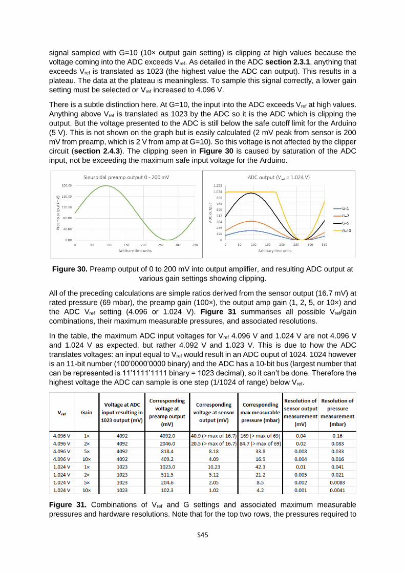
S45
signal sampled with G=10 (10× output gain setting) is clipping at high values because the
voltage coming into the ADC exceeds Vref. As detailed in the ADC section 2.3.1, anything that
exceeds Vref is translated as 1023 (the highest value the ADC can output). This results in a
plateau. The data at the plateau is meaningless. To sample this signal correctly, a lower gain
setting must be selected or Vref increased to 4.096 V.
There is a subtle distinction here. At G=10, the input into the ADC exceeds Vref at high values.
Anything above Vref is translated as 1023 by the ADC so it is the ADC which is clipping the
output. But the voltage presented to the ADC is still below the safe cutoff limit for the Arduino
(5 V). This is not shown on the graph but is easily calculated (2 mV peak from sensor is 200
mV from preamp, which is 2 V from amp at G=10). So this voltage is not affected by the clipper
circuit (section 2.4.3). The clipping seen in Figure 30 is caused by saturation of the ADC
input, not be exceeding the maximum safe input voltage for the Arduino.
Figure 30. Preamp output of 0 to 200 mV into output amplifier, and resulting ADC output at
various gain settings showing clipping.
All of the preceding calculations are simple ratios derived from the sensor output (16.7 mV) at
rated pressure (69 mbar), the preamp gain (100×), the output amp gain (1, 2, 5, or 10×) and
the ADC Vref setting (4.096 or 1.024 V). Figure 31 summarises all possible Vref/gain
combinations, their maximum measurable pressures, and associated resolutions.
In the table, the maximum ADC input voltages for Vref 4.096 V and 1.024 V are not 4.096 V
and 1.024 V as expected, but rather 4.092 V and 1.023 V. This is due to how the ADC
translates voltages: an input equal to Vref would result in an ADC ouput of 1024. 1024 however
is an 11-bit number (100’0000’0000 binary) and the ADC has a 10-bit bus (largest number that
can be represented is 11’1111’1111 binary = 1023 decimal), so it can’t be done. Therefore the
highest voltage the ADC can sample is one step (1/1024 of range) below Vref.
Figure 31. Combinations of Vref and G settings and associated maximum measurable
pressures and hardware resolutions. Note that for the top two rows, the pressures required to
S46
obtain the displayed voltages exceed the maximum rating for the PX26-001GV pressure
transducer and may damage it. For completeness, we should also mention that the maximum
measurable pressures in the table are technically not completely correct. In reality they are
slightly lower than shown but extend slightly below zero into negative pressures. So for
example, at Vref=1.024V and G=1 the measurable range is not 0.0 to 42.3 mbar as shown, but
-1.0 to 41.3 mbar. This is due to how logical zero is defined with respect to actual zero pressure
(see section 2.4.3.1 and Figure 49).
A final remark in this section: since decreasing Vref from 4.096 V to 1.024 V has an effect
effectively the same as increasing gain (amplification) by 4×, then why not simply have only
one voltage reference (say 4.096 V) and instead add more output amp gain settings? The
reason is purely historical. During the development of the CRAB both the 4.096 and 1.024 V
references were considered and included in the prototype with a MOSFET relay to switch
between them. As the prototype circuit on the breadboard grew in size and attention was
focused on other parts of it, the two voltage references were forgotten and remained put. Then
programming of the microcontroller (CRAB Control) was begun and the two separate voltage
references were rediscovered. By then, there was no more room on the existing breadboard
layout to add additional output amp gain settings (without dismantling and rebuilding the
prototype), the deadline was fast approaching (so no dismantling and rebuilding), there was
concern that there might not be enough available signal pins on the Arduino board to control
the additional gain settings (as it turns out, there are), and the prototype worked well enough
as it was. As a result, the CRAB v0.1 is stuck with the two voltage references. A future version
of the CRAB may well dispense with the 1.024 V reference and have additional gain settings
instead. Meanwhile, it may be best to think of the 4.096 V to 1.024 V switch as adding a 4×
gain stage in series with the existing 1, 2, 5, or 10× main output amp gain.
2.4.2 Signal shifter
In all of the above, various amplification settings (or Vref settings) were used to “zoom in” into
pressure data and obtain high resolutions. This is all very well if the signal of interest is
relatively close to the baseline (0 mV from sensor or 0 mbar pressure). Figure 32 shows
simulated data for an acquisition run measuring the pressure of gas bubbles being pushed
through a needle into a fluid. The sensor output (and hence pressure) is quite close to zero
and the region of interest (between 1 and 3 mV from the sensor therefore 100 to 300 mV from
preamp, corresponding to 1 mV / 16.7 mV × 69 mbar = 4.1 mbar and 3 mV / 16.7 mV × 69
mbar = 12.4 mbar) is well amplified (with Vref = 1.024 V) at G=1× and G=2× settings. For higher
gain settings, the data clips (exceeds maximum ADC input voltage) and results in plateaus in
the plots. But the G=1× or G=2× settings give a good resolution.
Figure 32. Simulated preamp output with small swing but close to zero. At least some of the
Vref/gain combinations are able to amplify this sufficiently to get a good resolution but without
the data clipping.
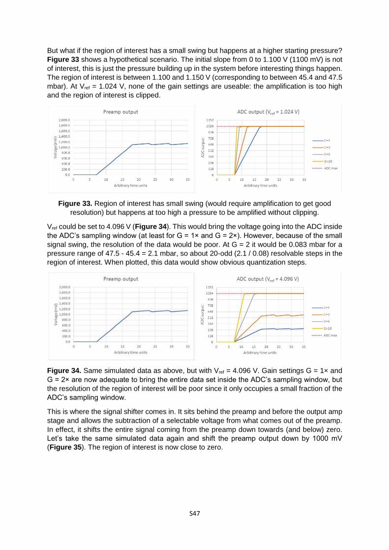
S47
But what if the region of interest has a small swing but happens at a higher starting pressure?
Figure 33 shows a hypothetical scenario. The initial slope from 0 to 1.100 V (1100 mV) is not
of interest, this is just the pressure building up in the system before interesting things happen.
The region of interest is between 1.100 and 1.150 V (corresponding to between 45.4 and 47.5
mbar). At Vref = 1.024 V, none of the gain settings are useable: the amplification is too high
and the region of interest is clipped.
Figure 33. Region of interest has small swing (would require amplification to get good
resolution) but happens at too high a pressure to be amplified without clipping.
Vref could be set to 4.096 V (Figure 34). This would bring the voltage going into the ADC inside
the ADC’s sampling window (at least for G = 1× and G = 2×). However, because of the small
signal swing, the resolution of the data would be poor. At G = 2 it would be 0.083 mbar for a
pressure range of 47.5 - 45.4 = 2.1 mbar, so about 20-odd (2.1 / 0.08) resolvable steps in the
region of interest. When plotted, this data would show obvious quantization steps.
Figure 34. Same simulated data as above, but with Vref = 4.096 V. Gain settings G = 1× and
G = 2× are now adequate to bring the entire data set inside the ADC’s sampling window, but
the resolution of the region of interest will be poor since it only occupies a small fraction of the
ADC’s sampling window.
This is where the signal shifter comes in. It sits behind the preamp and before the output amp
stage and allows the subtraction of a selectable voltage from what comes out of the preamp.
In effect, it shifts the entire signal coming from the preamp down towards (and below) zero.
Let’s take the same simulated data again and shift the preamp output down by 1000 mV
(Figure 35). The region of interest is now close to zero.
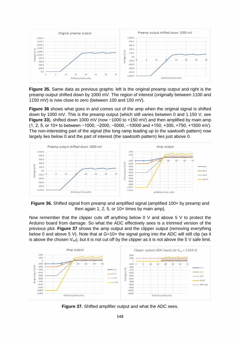
S48
Figure 35. Same data as previous graphs: left is the original preamp output and right is the
preamp output shifted down by 1000 mV. The region of interest (originally between 1100 and
1150 mV) is now close to zero (between 100 and 150 mV).
Figure 36 shows what goes in and comes out of the amp when the original signal is shifted
down by 1000 mV. This is the preamp output (which still varies between 0 and 1.150 V, see
Figure 33), shifted down 1000 mV (now −1000 to +150 mV) and then amplified by main amp
(1, 2, 5, or 10× to between −1000, −2000, −5000, −10000 and +150, +300, +750, +1500 mV).
The non-interesting part of the signal (the long ramp leading up to the sawtooth pattern) now
largely lies below 0 and the part of interest (the sawtooth pattern) lies just above 0.
Figure 36. Shifted signal from preamp and amplified signal (amplified 100× by preamp and
then again 1, 2, 5, or 10× times by main amp).
Now remember that the clipper cuts off anything below 0 V and above 5 V to protect the
Arduino board from damage. So what the ADC effectively sees is a trimmed version of the
previous plot. Figure 37 shows the amp output and the clipper output (removing everything
below 0 and above 5 V). Note that at G=10× the signal going into the ADC will still clip (as it
is above the chosen Vref), but it is not cut off by the clipper as it is not above the 5 V safe limit.
Figure 37. Shifted amplifier output and what the ADC sees.
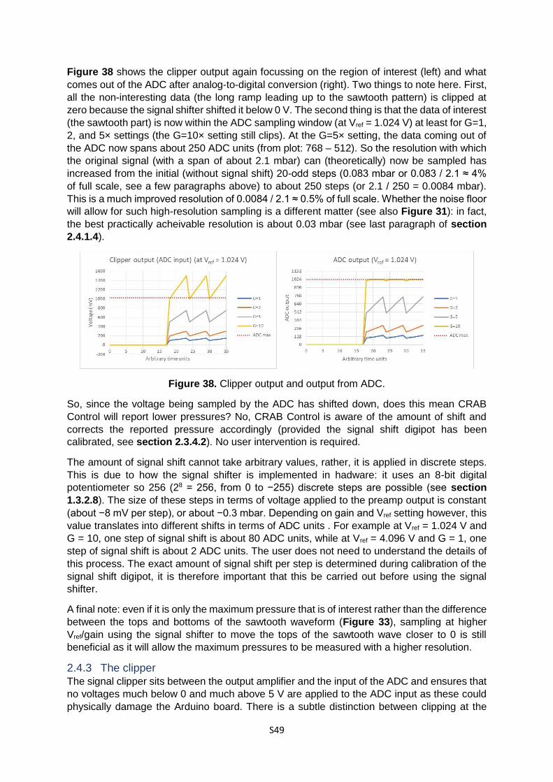
S49
Figure 38 shows the clipper output again focussing on the region of interest (left) and what
comes out of the ADC after analog-to-digital conversion (right). Two things to note here. First,
all the non-interesting data (the long ramp leading up to the sawtooth pattern) is clipped at
zero because the signal shifter shifted it below 0 V. The second thing is that the data of interest
(the sawtooth part) is now within the ADC sampling window (at Vref = 1.024 V) at least for G=1,
2, and 5× settings (the G=10× setting still clips). At the G=5× setting, the data coming out of
the ADC now spans about 250 ADC units (from plot: 768 – 512). So the resolution with which
the original signal (with a span of about 2.1 mbar) can (theoretically) now be sampled has
increased from the initial (without signal shift) 20-odd steps (0.083 mbar or 0.083 / 2.1 ≈ 4%
of full scale, see a few paragraphs above) to about 250 steps (or 2.1 / 250 = 0.0084 mbar).
This is a much improved resolution of 0.0084 / 2.1 ≈ 0.5% of full scale. Whether the noise floor
will allow for such high-resolution sampling is a different matter (see also Figure 31): in fact,
the best practically acheivable resolution is about 0.03 mbar (see last paragraph of section
2.4.1.4).
Figure 38. Clipper output and output from ADC.
So, since the voltage being sampled by the ADC has shifted down, does this mean CRAB
Control will report lower pressures? No, CRAB Control is aware of the amount of shift and
corrects the reported pressure accordingly (provided the signal shift digipot has been
calibrated, see section 2.3.4.2). No user intervention is required.
The amount of signal shift cannot take arbitrary values, rather, it is applied in discrete steps.
This is due to how the signal shifter is implemented in hadware: it uses an 8-bit digital
potentiometer so 256 (28 = 256, from 0 to −255) discrete steps are possible (see section
1.3.2.8). The size of these steps in terms of voltage applied to the preamp output is constant
(about −8 mV per step), or about −0.3 mbar. Depending on gain and Vref setting however, this
value translates into different shifts in terms of ADC units . For example at Vref = 1.024 V and
G = 10, one step of signal shift is about 80 ADC units, while at Vref = 4.096 V and G = 1, one
step of signal shift is about 2 ADC units. The user does not need to understand the details of
this process. The exact amount of signal shift per step is determined during calibration of the
signal shift digipot, it is therefore important that this be carried out before using the signal
shifter.
A final note: even if it is only the maximum pressure that is of interest rather than the difference
between the tops and bottoms of the sawtooth waveform (Figure 33), sampling at higher
Vref/gain using the signal shifter to move the tops of the sawtooth wave closer to 0 is still
beneficial as it will allow the maximum pressures to be measured with a higher resolution.
2.4.3 The clipper
The signal clipper sits between the output amplifier and the input of the ADC and ensures that
no voltages much below 0 and much above 5 V are applied to the ADC input as these could
physically damage the Arduino board. There is a subtle distinction between clipping at the

S50
ADC input (where the input exceeds Vref but not 5 V and so the ADC translates everything
above this limit as ‘1023’) and the intentional clipping of everything below 0 and above 5 V to
protect the Arduino microcontroller board. This is illustrated in the following. In practical terms,
both forms of clipping will have the same effect on the data in that plateaus will be seen.
Figure 39 shows a hypothetical amplifier output for all gains (left) and the resulting output of
the clipper. Everything below about 0 and above about 5 V has been cut off, or “clipped”. This
signal is safe to feed into the Arduino’s ADC.
Figure 39. Amp output −5 to +6 V and corresponding clipper output.
But when the ADC’s Vref is set to 1.024 V, the other form of clipping alluded to earlier occurs.
With Vref equal to 1.024 V, the ADC maps all voltages between 0 and 1.024 V to a range of
values between 0 and 1024. While there is no signal component below 0 V anymore, anything
above Vref (1.024 V) will be translated as ‘1023’ and therefore another plateau is introduced
(Figure 40).
Figure 40. Same data as Figure 39 (left) clipped by the ADC due to exceeding Vref.
As a result, only the G=1 data is undistorted. The situation could be remedied by either a)
increasing Vref to 4.096 V (this widens the ADC window, but decreases resolution, although a
higher G setting might then be available, which would again increase resolution), or b) shifting
the signal down so that the G=2 (and maybe also 5, and 10) peaks fit into the ADC window.
This would clip the baseline but would bring the peaks back inside the ADC window.

S51
2 CRAB Control v0.1 software manual
2.1 Introduction CRAB Control is the software that runs on the Arduino Nano microcontroller, controls the
CRAB hardware and provides a user interface which allows interaction with the CRAB. The
following text describes the setting up and use of the CRAB v0.1 under CRAB Control v0.1.
CRAB Control is simple by necessity: the memory available on-board the Arduino Nano is
rather limited. As it is, version 0.1 of the firmware already uses 96 % of available memory.
CRAB control allows for calibration of the sensor response from the CRAB, selection of data
acquisition parameters and pressure data acquisition.
Communication with the user is via a text-only terminal. Mouse input is not supported. A future
version of CRAB Control will include dedicated client software running on the attached
computer. This will allow for far more flexible and user-friendly operation than is possible with
the terminal-only version.
2.2 First-time setup
2.2.1 Power supply
The CRAB v0.1 has no protection against excessive power supply voltages or supplies of the
wrong polarity. Excessive voltages may, and wrong polarity will destroy the CRAB. Only use
the CRAB with a suitable power supply.
When powering the CRAB before use, the external power supply should be plugged in first,
followed by USB connection to the PC. If the USB connection is made first, followed by
external power, the CRAB may not work properly. If the USB cable is connected but the user
forgets to connect the external power supply, CRAB Control and the CRAB will appear to
function, but calibration and pressure readings will fail (see section 1.3.2.1).
This is due to how the different parts of the CRAB are powered internally: a USB connection
to the computer will power the Arduino microcontroller but not the rest of the electronics
(sensor, preamp, null offset digipot, signal shifter, voltage references, Vref switch and amplifier).
CRAB Control will run and interact with the user as normal but will not be aware that the
electronics it is trying to control are unpowered. As a result, attempted pressure readings will
be meaningless readings of random floating voltages. Additionally, CRAB Control v0.1
initializes some of the CRAB’s signal processing components to known values on start-up. If
external power is not connected when it does this, this initialization will not happen (but CRAB
Control will assume it did) and CRAB Control may work incorrectly even if external power is
applied subsequently. If a USB connection to a PC was in place before the external power
supply is plugged in, the CRAB should be reset (using the reset button) before use. This will
ensure the correct initialization of the CRAB’s electronics.
The external power supply on the other hand, powers both the CRAB’s signal processing
electronics and the Arduino microcontroller, so applying external power before USB power will
ensure correct initialization of the CRAB. In fact, the CRAB could be used with a USB cable
with the +5 V wire cut as it is not dependent on USB power at all, and this will be implemented
in a future version of the CRAB.
2.2.2 Hardware calibration Hardware calibration is a one-time procedure in which multi-turn potentiometers VR1 and VR2
on the printed circuit board are adjusted to the correct values. This procedure must be carried
out after assembling the CRAB and prior to first use.

S52
VR2 (DC bias for null offset adjust circuit) is adjusted so that a voltage of approximately 200
mV is measured at TP2 (test point 2) relative to circuit ground (e.g. the metal enclosure of the
USB socket). VR1 (control voltage for null offset adjust circuit) is adjusted so that
approximately 100 mV is measured at TP1 relative to circuit ground. The reason for these
values is given in section 1.3.2.7.
VR1 must be adjusted before any data has been written to digipot IC2 by software. The reason
for this is that, when first powered up, the MCP 4151-103 digipot (IC2) defaults to its midpoint
setting and it is this midpoint setting that is assumed to be in force during calibration of VR1.
The best way to ensure that this condition is met is to remove all power from the CRAB (USB
cable and external power), then reconnect the external power supply only and carry out the
calibration of VR1.
Should VR1 and VR2 they need re-adjusting at a later point for any reason (they shouldn’t),
recalibration of the CRAB will also be necessary (section 2.3.4.2).
2.3 Using the CRAB Control v0.1 software
2.3.1 Connecting to a computer The CRAB communicates with the computer via a USB-emulated serial protocol and the user
interface is via a simple serial terminal window. Any computer architecture or operating system
should therefore be suitable for use with the CRAB so long as suitable serial terminal
emulation software is available. The serial terminal emulator must support ANSI escape
sequences and 115200 bps serial communications. This author used and recommends the
well-established PuTTY v0.70 software (www.putty.org). This author is also not familiar with
the setting up of peripherals or software packages on computers other than Windows PCs and
is unable to offer any guidance in this respect. The following applies to Windows platforms.
For the PC to recognize the CRAB, Arduino drivers must be installed. This is most easily done
by downloading and installing the Arduino IDE (www.arduino.cc), which is also required to
upload CRAB Control to the microcontroller board. The communications port number (COM
port) that the CRAB is assigned upon connecting to a PC can be found in Window’s Device
Manager under “Ports (COM & LPT)”. The CRAB identifies itself as “Arduino Nano”. If this
entry is not found under “Ports”, either the Arduino drivers have not been installed correctly or
an Arduino clone is being used rather than the genuine Arduino Nano. An Arduino clone will
work with the CRAB but requires a separate driver: refer to the documentation for your specific
clone.
The communication settings for PuTTY (or other terminal emulator) are 115200 8N1 (115200
bits/s, 8 data bits, no parity, 1 stop bit). If the CRAB is always plugged into the same USB port,
the COM port assignment should remain the same, but it can change if a different USB port is
used. The communication settings can be saved as a “session” in PuTTY for easy recall.
Text instructions are displayed in the terminal window and user interaction is via keyboard key
presses (no mouse support). Hotkeys (keyboard keys which result in some action or other in
the context of the current menu) are indicated by square brackets (“[“ and “]”). For instance,
“[M]ode cycle” indicates that pressing the “m” key will cycle through available averaging modes.
Both lower and upper case key presses are accepted.
Text to be displayed to the user is sent to the terminal once, after which it is the terminal
software’s job to keep it on screen for as long as needed. CRAB Control does not continuously
update the terminal display window. This is unlike e.g. a video monitor, which can be
unplugged and reconnected to the computer and will resume displaying the same screen it
was displaying before unplugging.

S53
CRAB Control has no way of knowing what the terminal is or isn’t displaying: it assumes that
text it has sent to the terminal is being displayed as intended. What this means is that if any
text sent by CRAB Control to the terminal is lost (due to e.g. the USB cable being unplugged,
the terminal window closed, or the terminal window being opened after a text transmission
from CRAB Control), it will not be displayed in the terminal window and CRAB Control will not
know that it isn’t being displayed. The CRAB is still operating correctly even though the
terminal screen may be blank or incomplete.
Selecting a menu option or pressing [ESC] (to return to previous menu: not all menus allow
this) will restore at least some of the display. Pressing <ENTER> on the main menu redraws
the screen completely. Alternatively, pressing the reset button on the CRAB will also redraw
the terminal screen (but any unsaved settings will be lost).
2.3.2 Menu structure The CRAB Control menu is hierarchical with a tree structure. The main menu consists of the
major groups “Run”, “Settings”, and “Calibration”. Two other options in the main menu are
“Remote operation” (for communication with a dedicated PC client application – not yet
implemented) and “Info” (provides version and author information). Navigation is by pressing
keyboard keys indicated between square brackets. Pressing [ENTER] in the main menu
redraws the screen. This is useful if the terminal screen was corrupted for any reason (see
section 2.3.1). Pressing [ESC] from the major groups returns to the main menu.
Selection of actions/submenus inside the major groups is analogous, by pressing the
associated keyboard key. Once an action has been selected, the user follows the instructions
on the screen. Depending on the action, [ESC] may sometimes be used to cancel/exit (this is
indicated on screen if it is the case). Otherwise, the action must be followed through to the
end. On completion of an action (or cancelling with [ESC] if allowed), CRAB Control jumps
back to the main menu, rather than the previous submenu. This behaviour differs from the
more familiar behaviour of tree-like menu structures (which jump back to the previous
submenu) and will be amended in a future version of CRAB Control. For consistency, the
option to [ESC] from any action may also be added in a future version of the firmware.
Figure 41 shows the CRAB Control v0.1 menu tree. Practical usage of CRAB control, from
selection of operating settings, to calibration, to experimental data acquisition, is described
below. Individual menu actions are described individually in section 2.4.
Figure 41. CRAB Control menu tree. The cyan boxes represent main menu groups, the
orange boxes the associated submenus/actions.
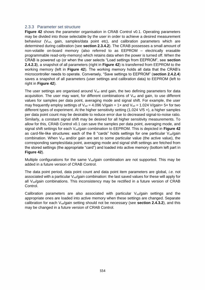
S54
2.3.3 Parameter set structure Figure 42 shows the parameter organisation in CRAB Control v0.1. Operating parameters
may be divided into those selectable by the user in order to achieve a desired measurement
behaviour (Vref, gain, samples/data point etc), and calibration parameters which are
determined during calibration (see section 2.3.4.2). The CRAB possesses a small amount of
non-volatile on-board memory (also referred to as EEPROM – electrically erasable
programmable read-only-memory) which retains data when the power is turned off. When the
CRAB is powered up (or when the user selects “Load settings from EEPROM”, see section
2.4.2.3), a snapshot of all parameters (right in Figure 42) is transferred from EEPROM to the
working memory (left in Figure 42). The working memory holds all data that the CRAB’s
microcontroller needs to operate. Conversely, “Save settings to EEPROM” (section 2.4.2.4)
saves a snapshot of all parameters (user settings and calibration data) to EEPROM (left to
right in Figure 42).
The user settings are organised around Vref and gain, the two defining parameters for data
acquisition. The user may want, for different combinations of Vref and gain, to use different
values for samples per data point, averaging mode and signal shift. For example, the user
may frequently employ settings of Vref = 4.096 V/gain = 1× and Vref = 1.024 V/gain= 5× for two
different types of experiment. At the higher sensitivity setting (1.024 V/5 ×), a higher samples
per data point count may be desirable to reduce error due to decreased signal-to-noise ratio.
Similarly, a constant signal shift may be desired for all higher sensitivity measurements. To
allow for this, CRAB Control v0.1 can save the samples per data point, averaging mode, and
signal shift settings for each Vref/gain combination to EEPROM. This is depicted in Figure 42
as card-file-like structures: each of the 8 “cards” holds settings for one particular Vref/gain
combination. When Vref and/or gain are set to some particular value (the active value), the
corresponding samples/data point, averaging mode and signal shift settings are fetched from
the stored settings (the appropriate “card”) and loaded into active memory (bottom left part in
Figure 42).
Multiple configurations for the same Vref/gain combination are not supported. This may be
added in a future version of CRAB Control.
The data point period, data point count and data point item parameters are global, i.e. not
associated with a particular Vref/gain combination: the last saved values for these will apply for
all Vref/gain combinations. This inconsistency may be rectified in a future version of CRAB
Control.
Calibration parameters are also associated with particular Vref/gain settings and the
appropriate ones are loaded into active memory when these settings are changed. Separate
calibration for each Vref/gain setting should not be necessary (see section 2.4.3.2), and this
may be changed in a future version of CRAB Control.
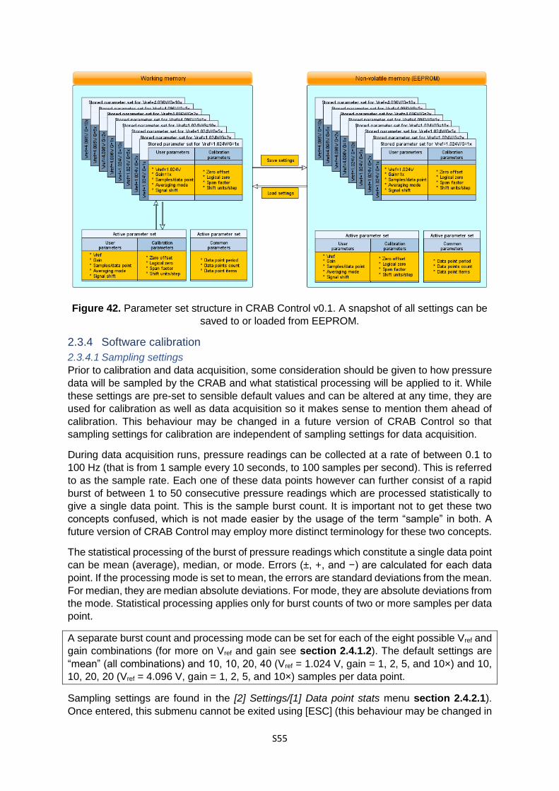
S55
Figure 42. Parameter set structure in CRAB Control v0.1. A snapshot of all settings can be
saved to or loaded from EEPROM.
2.3.4 Software calibration
2.3.4.1 Sampling settings
Prior to calibration and data acquisition, some consideration should be given to how pressure
data will be sampled by the CRAB and what statistical processing will be applied to it. While
these settings are pre-set to sensible default values and can be altered at any time, they are
used for calibration as well as data acquisition so it makes sense to mention them ahead of
calibration. This behaviour may be changed in a future version of CRAB Control so that
sampling settings for calibration are independent of sampling settings for data acquisition.
During data acquisition runs, pressure readings can be collected at a rate of between 0.1 to
100 Hz (that is from 1 sample every 10 seconds, to 100 samples per second). This is referred
to as the sample rate. Each one of these data points however can further consist of a rapid
burst of between 1 to 50 consecutive pressure readings which are processed statistically to
give a single data point. This is the sample burst count. It is important not to get these two
concepts confused, which is not made easier by the usage of the term “sample” in both. A
future version of CRAB Control may employ more distinct terminology for these two concepts.
The statistical processing of the burst of pressure readings which constitute a single data point
can be mean (average), median, or mode. Errors (±, +, and −) are calculated for each data
point. If the processing mode is set to mean, the errors are standard deviations from the mean.
For median, they are median absolute deviations. For mode, they are absolute deviations from
the mode. Statistical processing applies only for burst counts of two or more samples per data
point.
A separate burst count and processing mode can be set for each of the eight possible Vref and
gain combinations (for more on Vref and gain see section 2.4.1.2). The default settings are
“mean” (all combinations) and 10, 10, 20, 40 (Vref = 1.024 V, gain = 1, 2, 5, and 10×) and 10,
10, 20, 20 (Vref = 4.096 V, gain = 1, 2, 5, and 10×) samples per data point.
Sampling settings are found in the [2] Settings/[1] Data point stats menu section 2.4.2.1).
Once entered, this submenu cannot be exited using [ESC] (this behaviour may be changed in
S56
a future version of CRAB Control). If the user does not wish to change any settings, pressing
[ENTER] through all steps will keep the current values and eventually exit the submenu. The
default settings should be suitable for most applications but can be adjusted as required.
After setting the desired sample burst counts and processing modes for all Vref and gain
combinations, these will be used in subsequent calibration and data acquisition operations.
The sample burst counts and processing modes can be saved to EEPROM (see sections
2.4.2.3 and 2.4.2.4).
2.3.4.2 Calibration
On first use, the CRAB will assume an ideal calibration taken from the PX26-001GV sensor’s
datasheet. This should result in pressure readings close to true but due to manufacturing
variabilities, and obviously if a pressure transducer other than the PX26-001GV is being used,
calibration needs to be carried out using a reference manometer. If a pressure transducer
other than the PX26-001GV is being used, the transducer’s full scale voltage and pressure
need to be set in the relevant menu prior to calibration (see section 2.4.3.4). All pressures in
CRAB Control v0.1 are in millibar (mbar). One mbar is equal to 100 Pa (or 1 bar equal to 100
kPa). A future version of Crab Control may include the ability to choose between different
pressure units.
The calibration submenus will ask the user to apply a range of pressures to the sensor and
the CRAB will calculate the required correction factors so that the pressure readings from the
CRAB are equal to the pressure readings from the reference manometer. The quality of the
calibration will depend on the accuracy of the reference manometer. Cheap digital
manometers are widely available from many internet retailers.
Calibration should not need to be repeated particularly often. During development of the CRAB,
it was noted that usage of calibration settings saved one day earlier resulted in pressure
readings which were off by a fraction of a mbar compared to the readings of the handheld
manometer. This is a very small difference and should not be of much practical consequence.
The reason is unknown, perhaps a temperature effect. Due to the questionable quality of the
handheld manometer used as a reference in the first place (and lack of any accompanying
accuracy/precision specifications), the source of the discrepancy may just as well lie with the
reference as with the CRAB. A future version of the CRAB may include circuitry to compensate
for temperature. For the time being, the CRAB should be calibrated at the temperature it is to
be used at.
The calibration submenu contains four items, three of which are part of a routine calibration
and need to be carried out in a specific order. These are, in order, [1] Zero offset calibration,
and [2] Span factor calibration. [3] Signal shift digipot calibration needs only to be carried out
if the signal shifter is used. For a more detailed explanation, see section 2.4.3.
Calibrations are performed for all eight possible Vref/gain combinations separately and sample
burst count and processing modes set for these combinations (see section 2.3.4.1) are used.
The CRAB will sample 10 data points (at their respective burst counts/processing modes),
average them, and calculate calibration factors from this.
The zero offset calibration lets CRAB Control know what signal to expect from the sensor at
zero differential pressure (when the sensor is open to the atmosphere). The user should
disconnect any pressure tubing from the sensor (or otherwise vent the setup) before
proceeding. The calibration procedure will scan all Vref/gain combinations in turn and adjust
the internal zero offset digipot to bring the ADC reading as close as possible to ADC logical
zero (see section 2.4.3.1). For more detail on zero offset digipot, see the CRAB hardware
S57
manual (section 1.3.2.7). When finished, the calibration procedure will prompt the user to
press any key and then return to the main menu.
The span factor calibration measures the slope of the voltage vs pressure response curve
from the sensor and compares it to the value in the sensor datasheet. This is done separately
for each of the eight possible Vref/gain combinations. Two data points are necessary: zero
pressure (which has been dealt with during zero offset calibration: this is why zero offset
calibration must be performed first), and a point somewhere between zero and the maximum
allowed pressure for the current Vref/gain combination. To maximize the accuracy of the
calibration, the second point should be near the maximum allowed pressure. CRAB Control
will ask the user to apply specified pressures to the sensor and enter the actual pressure
applied (read from the reference manometer). From this, CRAB Control calculates and
displays the calibration factors for each Vref/gain combination. All calibration factors should be
close to 1.00.
Finally, the signal shift digipot calibration serves to determine the amount of signal shift that
the internal signal shift digipot will apply to the signal from the sensor for each Vref/gain
combination. See section 1.3.2.8 for more information. To do this, a test pressure is applied
to the sensor and the signal shift digipot is dialled to whichever setting is necessary to bring
the ADC input close to ADC logical zero (see section 2.4.3.1). The ADC range traversed is
divided by the number of discrete digipot steps required to accomplish this to give a value (in
ADC units per step) describing how much each step of signal shift affects the ADC input.
CRAB Control needs to know this to display the correct pressure when signal shift is applied.
Same as for span factor calibration, accuracy is maximized if the range between initial and
final ADC readings is as large as possible. CRAB Control will ask the user to apply a number
of test pressures (suitable for each Vref/gain combination) while carrying out this calibration.
Unlike span calibration, the user is not required to input the actual test pressure: since zero
offset and span calibration have already been carried out, CRAB Control measures the applied
test pressures itself. If the reference manometer is still attached to the system, it can be used
to check the quality of the calibration at the same time.
Since there are eight possible Vref/gain combinations, one could expect eight different test
pressures to be required during span and signal shift calibration. To minimize user annoyance,
the Vref/gain combinations are banded into groups with similar maximum pressures and
calibrations are carried out on the groups, rather than individual Vref/gain combinations. This
reduces the number of test pressures required to 3 for span calibration, and 4 for signal shift
digipot calibration. It is also the reason why the calibrations are carried out in a seemingly
random order.
The test groups have been specifically chosen for the PX26-001GV sensor and are fixed in
software. A sensor with a wider pressure range will not be calibrated optimally (since a smaller
portion of its range will be used) and a sensor with a smaller pressure range may require
pressure that exceed its rated limits. The calibration algorithms will be rewritten in a future
version of CRAB Control to account for pressure transducers other than the PX26-001GV.
Upon finishing, all calibration settings can be saved to EEPROM (section 2.4.2.4). The fourth
item in the calibration menu (sensor range) should not be used during routine calibration. It
was added last-minute (see section 1.3.1) and is for adapting pressure transducers other than
the PX26-001GV to work with the CRAB (see section 2.4.3.4).
S58
2.3.5 Measuring pressure data
2.3.5.1 Parameter selection
Following calibration, the parameters for data acquisition need to be set. All of these, bar one,
are found in the [1] Run submenu. The missing one is found in the [2] Settings submenu. This
inconsistency is an artefact of hectic last-minute development work on CRAB Control and a
future version will have the menus rearranged in a more logical fashion.
This is where it helps if the user has a rough idea of what behaviour to expect from the sample.
If the optimal parameters for the run are not set, parts of the data collected may clip (and be
useless) or the resolution may end up being poor for the data of interest (see section 2.3.1).
For an unknown sample, the general procedure is to set the CRAB to maximum range (and
therefore minimum resolution) by selecting Vref = 4.096 V and gain = 2× (rather than 1×, see
the following). At this Vref/gain combination, a maximum sensor output (16.7 mV) will be
amplified to 16.7 mV × 100 (preamp) × 2 (amp) = 3.34 V, which is well within the input range
of the ADC at Vref = 4.096 V (for details on the electronics see sections 1.3.2.5 and 1.3.2.9,
for a more in-depth explanation of the operating principles, see sections 2.2.2, 2.3.1, and
2.4.1). The Vref = 4.096 V / gain = 1× combination is not very useful for anything unless the
measured pressures are well above the rated maximum for the PX26-001GV sensor (which
may damage the sensor, unless a different sensor is used).
With these settings, an acquisition run is recorded, the data examined and the Vref/gain
adjusted accordingly for maximum resolution in the region of interest (see sections 2.4.1 and
2.4.2). This can be done by manually calculating the required parameters, or “by eye”, using
Run scouting.
2.3.5.1.1 Parameters selection: run scouting
Run scouting (see also section 2.4.1.4) is a useful little feature which records a short data run
of limited resolution, displays it on screen, and allows for visual manipulation of the displayed
pressure/time curve to maximise resolution and avoid clipping, while setting the corresponding
run parameters automatically. Iterating more than one consecutive scouting run (zeroing in,
so to say) may still be necessary to find the optimal combination of settings, but run scouting
should make parameter selection much more painless.
The run scouting submenu is found under [1] Run/[4] Run scouting. Initially, maximum range
(Vref = 4.096 V / gain = 2×) should be selected, zero signal shift, and a suitable run time. The
run time is set by entering either the sample rate (in Hz), or the sample period (in ms): these
two are reciprocals so setting one determines the other, and the total run time is determined
by the fixed number (100) of data points. In CRAB Control v0.1 the run time cannot be entered
directly by the user: this may be changed in a future version of the software. For the scouting
run, the CRAB must hold all acquired pressure data inside its on-board memory. Because this
is severely limited, only 100 data points can be recorded. The 100 data points are therefore
spaced over the sample rate/period selected by the user, and the run time is calculated
accordingly. For example, if a sample rate of 5 Hz (5 pressure readings per second) is selected,
this equals to a sample period of 200 ms (the interval between pressure readings) and a total
run time of 20 s (100 samples divided by 5 samples/second). If a sample period of 20 ms is
selected (one pressure reading every 20 ms), this equals to a sample rate of 50 Hz (1000 ms
divided by 20 ms) and a total run time of 2 s (100 samples divided by 50 samples/second).
The low available memory limits the resolution on the time axis, particularly for longer runs,
therefore detail in the pressure readings (for quickly changing pressures) may be missed or
aliasing (see section 2.4.2.1.1) may even occur. This is something to be aware of when using
run scouting.
S59
Once the initial Vref/gain/signal shift have been selected, the scout run is started at the same
time as whatever experiment the user is carrying out. A series of 100 data points is collected
(the time this takes being determined by the sample rate/period, see above) and the data is
displayed in a graph in the terminal window. Since the terminal window is text-only, the graph
is very simple and low-resolution. Data points are represented by hashes (“#”) and those that
clipped (during acquisition) are in red. The x-axis represents time (initially from 0 s to whatever
the run time of the scout run was) and the y-axis represents pressure. Note that the y-axis
limits show the range of pressures that can be recorded at a given Vref/gain/shift
combination. Entering the Run scouting menu and setting Vref/gain/shift parameters just to
peek at the y-axis, and then exiting, may be useful should the user need reminding of the
pressure limits of the current Vref/gain combination. While the x-axis can be zoomed into (so
that not all recorded data is displayed, see below), the y-axis always shows the entire
measurable pressure range (the range of pressures which results in an ADC output between
0 and 1023, for more detail see section 2.3.1) for the given Vref/gain/shift combination. See
Figure 49 for a summary of pressure ranges for all Vref/gain combinations.
The usefulness of run scouting lies in being able to display the scout data to show what it
would have looked like had it been recorded at a different Vref/gain/shift setting. Note the
parameter list area above the graph. This is divided into two sections: acquisition parameters
(the parameters that were used for recording the scout data), and display parameters (the
display parameters of the graph that the scout data is being displayed in). Changing any of
Vref, gain or shift using the indicated control keys changes the display parameters only and
redraws the graph. If, after changing a parameter, some of the acquired data points fall outside
the measurable window, they will be highlighted in red, meaning that they would have clipped
had the data been acquired with the display parameters. Data points which clipped during
acquisition and are therefore invalid (because their voltage exceeded the ADC input window)
will remain red even though it may be possible to move them inside the measurable window
by changing some of the display parameters.
Once the display parameters have been adjusted as required, the user can repeat the scouting
run. This copies the display parameter set into the acquisition parameters set, that is, pressure
data is re-acquired using the display parameters (which were chosen to display the previous
data set with) as acquisition parameters. The new data is displayed in a graph again, and the
process repeats: the user may continue adjusting display parameters and re-acquiring data
until satisfied, or they may exit run scouting. Pressing [ENTER] transfers the display
parameters into active acquisition parameters and returns to the main menu. Starting a proper
data acquisition run will now use those parameters. Pressing [ESC] returns to the main menu
and discards any changes that were made to Vref/gain/shift in the run scouting screen.
By default, the x-axis displays the entire length of scout data which was acquired. The x-axis
limits may be moved using the indicated control keys so that a detail of interest may be zoomed
into. It is possible to zoom out past the extent of recorded data. Unlike Vref, gain and shift,
which are updated to reflect the display values when [ENTER] is pressed in the run scouting
menu, the total run time for actual data acquisition is not modified by changing sample
rate/period (or by changing x-axis limits) in this menu: it must be set separately (see next
section). This behaviour may be changed in a future version of CRAB control.
2.3.5.1.2 Parameter selection: manual
Data acquisition parameters can also be set manually, and run time and sample rate/period
(for data acquisition run, not scout run) must be set manually. This is done using the remaining
options in the [1] Run menu.
S60
The sample rate or period is set in [1] Run/[1] Sample rate/period. The user can choose
whether to specify the sample rate or period: these two are reciprocals so one determines the
other. Unlike for run scouting, there is no limit on data points for actual data runs because the
pressure data is dumped into the terminal window (or log file, from which it can be copied into
other data processing software) and does not need to be held in on-board memory. See
section 2.4.1.1 for more detail.
Vref, gain and signal shifts for data acquisition are set manually from the [1] Run/[2] ADC VRef,
amp gain, signal shift submenu. The real-time sensor pressure is displayed at the bottom of
this screen. See section 2.4.1.2 for more detail.
The total data acquisition run time is set from the [1] Run/[3] Run time submenu. This can be
specified in total data points, or total time (seconds). If specified in number of data points, the
previously chosen sample rate will determine total run time. If specified in total time, the
previously chosen sample rate will determine the number of data points collected. Data
acquisition can be interrupted with a key press so it is convenient to choose a longer than
necessary run time and interrupt acquisition manually when sufficient data has been collected.
See sections 2.4.1.3 and 2.4.1.6 for more detail.
Finally, the data items to be logged during the data acquisition need to be specified: this is
done in submenu [1] Run/[5] Data items. The choices are time, pressure, error ±, error +, error
−, and clip warning (the first three and clip warning are selected by default). This determines
how much information on each acquired data point is dumped into the terminal window during
data acquisition. See section 2.4.1.5 for more detail.
2.3.5.2 Data acquisition
After deciding on sampling/statistical processing settings and acquisition parameters, the
actual data acquisition is a matter of a few key presses. The data acquisition run is started
using [1] Run/[6] Start run. A screen message advises the user to start data logging in their
terminal window. For all but the shortest of runs (where the few data points can be copied and
pasted out of the terminal into other software) it is convenient to use the serial terminal’s “data
logging” feature. This writes all data received from (and inserted by the user into) the serial
link into a file. In PuTTY, this feature is accessed from the configuration menu, under
Session/Logging. “Printable output” and “Flush log file frequently” should be selected. A log
file name and folder should be specified by the user (otherwise the file putty.log will be used
inside PuTTY’s installation folder). Using the &Y, &M, &D and &T placeholders (for current
year, month, day, and time) is a convenient way of making PuTTY automatically name log
files. For instance, “&Y&M&D-&T.log” might name a file “20190201-162210.log”.
After logging has been enabled, another key press in the terminal window displays all sampling
and acquisition parameters which will be used for the data acquisition run. The data acquisition
run is started with another key press. The acquired data (all items which were selected for
acquisition, see section 2.4.1.5) are now printed to screen and logged to the file specified in
PuTTY’s logging menu. The data acquisition stops automatically when the requested number
of data points has been measured (see section 2.4.1.3) or it can be stopped by pressing
[ESC].
After data acquisition is complete, logging should be disabled (by selecting “None” in PuTTY’s
logging options) to avoid polluting the log file with user key presses and text meant for menu
display. Additionally, if logging is not stopped, the log file will still be locked by PuTTY and
some applications may refuse to open it. Pressure data from CRAB Control is in CSV format
(comma separated values, essentially ASCII text with a specific formatting) so the log files can
be imported directly into any application that supports this format.
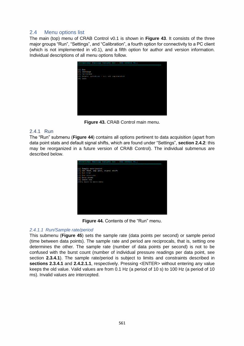
S61
2.4 Menu options list The main (top) menu of CRAB Control v0.1 is shown in Figure 43. It consists of the three
major groups “Run”, “Settings”, and “Calibration”, a fourth option for connectivity to a PC client
(which is not implemented in v0.1), and a fifth option for author and version information.
Individual descriptions of all menu options follow.
Figure 43. CRAB Control main menu.
2.4.1 Run The “Run” submenu (Figure 44) contains all options pertinent to data acquisition (apart from
data point stats and default signal shifts, which are found under “Settings”, section 2.4.2: this
may be reorganized in a future version of CRAB Control). The individual submenus are
described below.
Figure 44. Contents of the “Run” menu.
2.4.1.1 Run/Sample rate/period
This submenu (Figure 45) sets the sample rate (data points per second) or sample period
(time between data points). The sample rate and period are reciprocals, that is, setting one
determines the other. The sample rate (number of data points per second) is not to be
confused with the burst count (number of individual pressure readings per data point, see
section 2.3.4.1). The sample rate/period is subject to limits and constraints described in
sections 2.3.4.1 and 2.4.2.1.1, respectively. Pressing <ENTER> without entering any value
keeps the old value. Valid values are from 0.1 Hz (a period of 10 s) to 100 Hz (a period of 10
ms). Invalid values are intercepted.
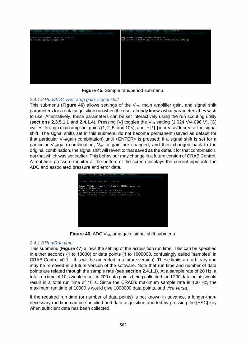
S62
Figure 45. Sample rate/period submenu.
2.4.1.2 Run/ADC Vref, amp gain, signal shift
This submenu (Figure 46) allows settings of the Vref, main amplifier gain, and signal shift
parameters for a data acquisition run when the user already knows what parameters they wish
to use. Alternatively, these parameters can be set interactively using the run scouting utility
(sections 2.3.5.1.1 and 2.4.1.4). Pressing [V] toggles the Vref setting (1.024 V/4.096 V), [G]
cycles through main amplifier gains (1, 2, 5, and 10×), and [+] / [-] increase/decrease the signal
shift. The signal shifts set in this submenu do not become permanent (saved as default for
that particular Vref/gain combination) until <ENTER> is pressed: if a signal shift is set for a
particular Vref/gain combination, Vref or gain are changed, and then changed back to the
original combination, the signal shift will revert to that saved as the default for that combination,
not that which was set earlier. This behaviour may change in a future version of CRAB Control.
A real-time pressure monitor at the bottom of the screen displays the current input into the
ADC and associated pressure and error data.
Figure 46. ADC Vref, amp gain, signal shift submenu.
2.4.1.3 Run/Run time
This submenu (Figure 47) allows the setting of the acquisition run time. This can be specified
in either seconds (1 to 10000) or data points (1 to 1000000, confusingly called “samples” in
CRAB Control v0.1 – this will be amended in a future version). These limits are arbitrary and
may be removed in a future version of the software. Note that run time and number of data
points are related through the sample rate (see section 2.4.1.1). At a sample rate of 20 Hz, a
total run time of 10 s would result in 200 data points being collected, and 200 data points would
result in a total run time of 10 s. Since the CRAB’s maximum sample rate is 100 Hz, the
maximum run time of 10000 s would give 1000000 data points, and vice versa.
If the required run time (or number of data points) is not known in advance, a longer-than-
necessary run time can be specified and data acquisition aborted by pressing the [ESC] key
when sufficient data has been collected.
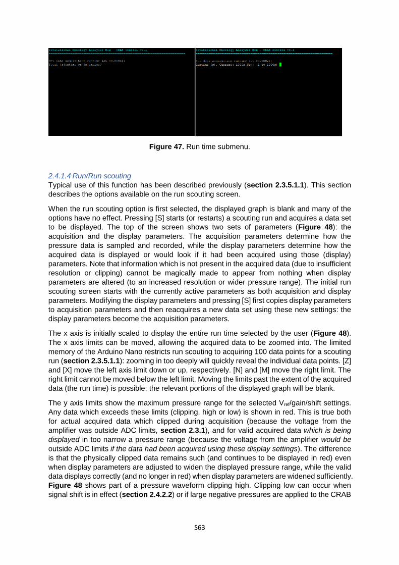
S63
Figure 47. Run time submenu.
2.4.1.4 Run/Run scouting
Typical use of this function has been described previously (section 2.3.5.1.1). This section
describes the options available on the run scouting screen.
When the run scouting option is first selected, the displayed graph is blank and many of the
options have no effect. Pressing [S] starts (or restarts) a scouting run and acquires a data set
to be displayed. The top of the screen shows two sets of parameters (Figure 48): the
acquisition and the display parameters. The acquisition parameters determine how the
pressure data is sampled and recorded, while the display parameters determine how the
acquired data is displayed or would look if it had been acquired using those (display)
parameters. Note that information which is not present in the acquired data (due to insufficient
resolution or clipping) cannot be magically made to appear from nothing when display
parameters are altered (to an increased resolution or wider pressure range). The initial run
scouting screen starts with the currently active parameters as both acquisition and display
parameters. Modifying the display parameters and pressing [S] first copies display parameters
to acquisition parameters and then reacquires a new data set using these new settings: the
display parameters become the acquisition parameters.
The x axis is initially scaled to display the entire run time selected by the user (Figure 48).
The x axis limits can be moved, allowing the acquired data to be zoomed into. The limited
memory of the Arduino Nano restricts run scouting to acquiring 100 data points for a scouting
run (section 2.3.5.1.1): zooming in too deeply will quickly reveal the individual data points. [Z]
and [X] move the left axis limit down or up, respectively. [N] and [M] move the right limit. The
right limit cannot be moved below the left limit. Moving the limits past the extent of the acquired
data (the run time) is possible: the relevant portions of the displayed graph will be blank.
The y axis limits show the maximum pressure range for the selected Vref/gain/shift settings.
Any data which exceeds these limits (clipping, high or low) is shown in red. This is true both
for actual acquired data which clipped during acquisition (because the voltage from the
amplifier was outside ADC limits, section 2.3.1), and for valid acquired data which is being
displayed in too narrow a pressure range (because the voltage from the amplifier would be
outside ADC limits if the data had been acquired using these display settings). The difference
is that the physically clipped data remains such (and continues to be displayed in red) even
when display parameters are adjusted to widen the displayed pressure range, while the valid
data displays correctly (and no longer in red) when display parameters are widened sufficiently.
Figure 48 shows part of a pressure waveform clipping high. Clipping low can occur when
signal shift is in effect (section 2.4.2.2) or if large negative pressures are applied to the CRAB
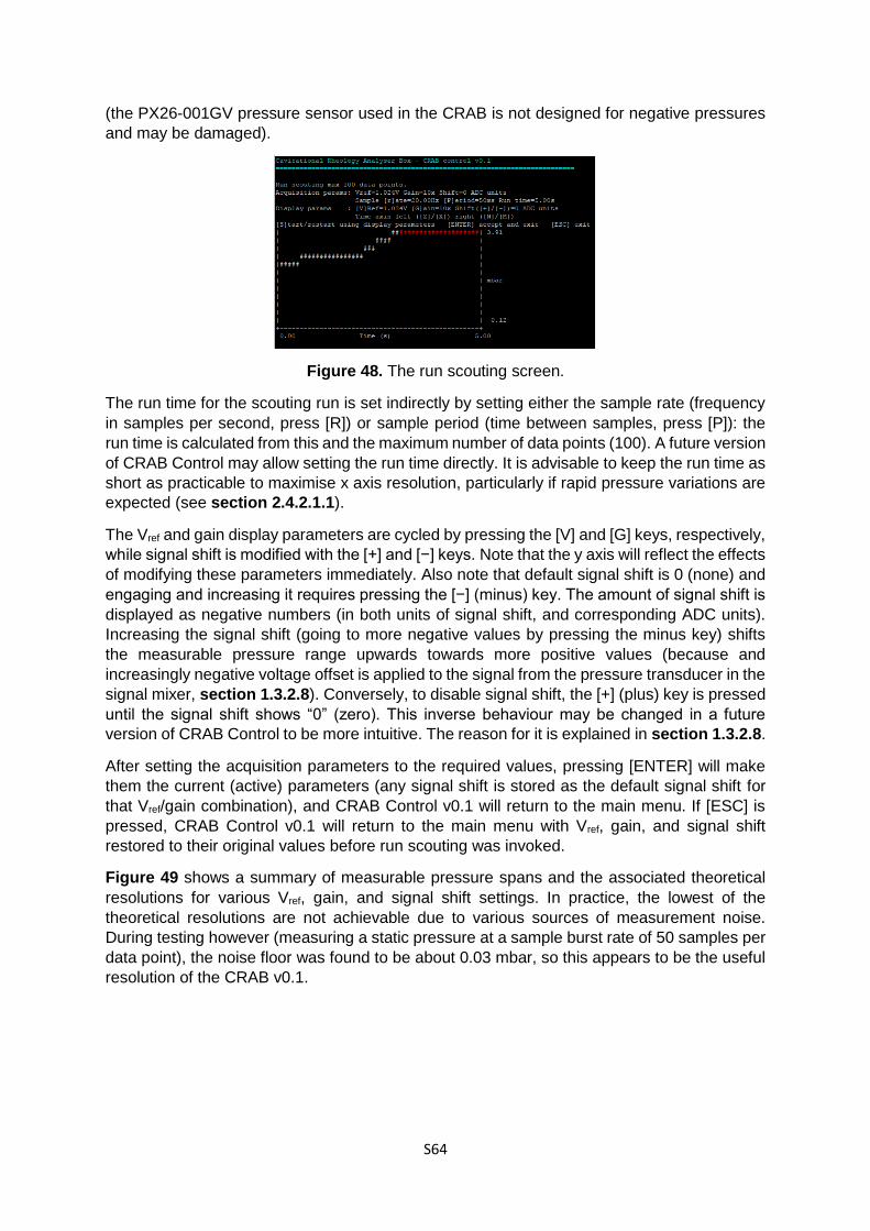
S64
(the PX26-001GV pressure sensor used in the CRAB is not designed for negative pressures
and may be damaged).
Figure 48. The run scouting screen.
The run time for the scouting run is set indirectly by setting either the sample rate (frequency
in samples per second, press [R]) or sample period (time between samples, press [P]): the
run time is calculated from this and the maximum number of data points (100). A future version
of CRAB Control may allow setting the run time directly. It is advisable to keep the run time as
short as practicable to maximise x axis resolution, particularly if rapid pressure variations are
expected (see section 2.4.2.1.1).
The Vref and gain display parameters are cycled by pressing the [V] and [G] keys, respectively,
while signal shift is modified with the [+] and [−] keys. Note that the y axis will reflect the effects
of modifying these parameters immediately. Also note that default signal shift is 0 (none) and
engaging and increasing it requires pressing the [−] (minus) key. The amount of signal shift is
displayed as negative numbers (in both units of signal shift, and corresponding ADC units).
Increasing the signal shift (going to more negative values by pressing the minus key) shifts
the measurable pressure range upwards towards more positive values (because and
increasingly negative voltage offset is applied to the signal from the pressure transducer in the
signal mixer, section 1.3.2.8). Conversely, to disable signal shift, the [+] (plus) key is pressed
until the signal shift shows “0” (zero). This inverse behaviour may be changed in a future
version of CRAB Control to be more intuitive. The reason for it is explained in section 1.3.2.8.
After setting the acquisition parameters to the required values, pressing [ENTER] will make
them the current (active) parameters (any signal shift is stored as the default signal shift for
that Vref/gain combination), and CRAB Control v0.1 will return to the main menu. If [ESC] is
pressed, CRAB Control v0.1 will return to the main menu with Vref, gain, and signal shift
restored to their original values before run scouting was invoked.
Figure 49 shows a summary of measurable pressure spans and the associated theoretical
resolutions for various Vref, gain, and signal shift settings. In practice, the lowest of the
theoretical resolutions are not achievable due to various sources of measurement noise.
During testing however (measuring a static pressure at a sample burst rate of 50 samples per
data point), the noise floor was found to be about 0.03 mbar, so this appears to be the useful
resolution of the CRAB v0.1.

S65
Figure 49. Pressure spans and theoretical resolutions for all Vref / gain combinations.
2.4.1.5 Run/Data items
In this screen (Figure 50) the user selects what data is dumped into the serial terminal during
acquisition. The choices are: time (a timestamp in milliseconds for the pressure reading),
pressure (the pressure for this data point, calculated based on selections in the data point
stats menu, sections 2.3.4.1 and 2.4.2.1), error +/− (symmetrical error), error + (asymmetrical
positive error), error − (asymmetrical negative error), and clip warning (a warning if the data
point was either a ‘0’ or ‘1023’ at the ADC input, see section 2.3.1).
Time, pressure, error +/− and clip warning are selected (‘Y’) by default. The items are toggled
on (‘Y’) and off (‘N’) by pressing the associated key in square brackets. The selection is
remembered for all subsequent data runs (but is not associated with a particular Vref / gain
combination) and can be saved to EEPROM as part of the active parameter set (section
2.3.3).
Figure 50. The data items selection screen.
2.4.1.6 Run/Start run
This begins the actual data acquisition run. On selecting this option, a message is displayed
prompting the user to enable logging on their terminal software (Figure 51). Pressing any key
displays all parameters in effect for the data acquisition. Another key press begins the actual
data acquisition.
During data acquisition, the data items chosen (section 2.4.1.5) are dumped into the terminal
screen at intervals specified by the sample rate (section 2.4.1.1). The data acquisition runs
until the specified run time is reached or [ESC] is pressed. When either occurs, the user should
disable logging in their terminal software to avoid unnecessary text being recorded in the log
file.
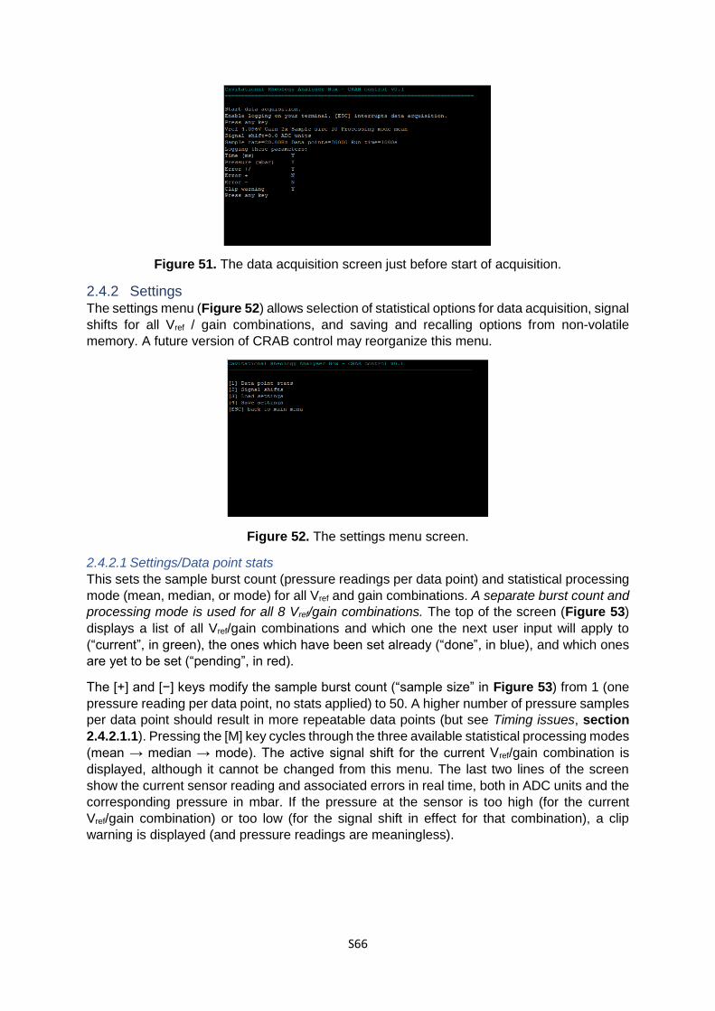
S66
Figure 51. The data acquisition screen just before start of acquisition.
2.4.2 Settings The settings menu (Figure 52) allows selection of statistical options for data acquisition, signal
shifts for all Vref / gain combinations, and saving and recalling options from non-volatile
memory. A future version of CRAB control may reorganize this menu.
Figure 52. The settings menu screen.
2.4.2.1 Settings/Data point stats
This sets the sample burst count (pressure readings per data point) and statistical processing
mode (mean, median, or mode) for all Vref and gain combinations. A separate burst count and
processing mode is used for all 8 Vref/gain combinations. The top of the screen (Figure 53)
displays a list of all Vref/gain combinations and which one the next user input will apply to
(“current”, in green), the ones which have been set already (“done”, in blue), and which ones
are yet to be set (“pending”, in red).
The [+] and [−] keys modify the sample burst count (“sample size” in Figure 53) from 1 (one
pressure reading per data point, no stats applied) to 50. A higher number of pressure samples
per data point should result in more repeatable data points (but see Timing issues, section
2.4.2.1.1). Pressing the [M] key cycles through the three available statistical processing modes
(mean → median → mode). The active signal shift for the current Vref/gain combination is
displayed, although it cannot be changed from this menu. The last two lines of the screen
show the current sensor reading and associated errors in real time, both in ADC units and the
corresponding pressure in mbar. If the pressure at the sensor is too high (for the current
Vref/gain combination) or too low (for the signal shift in effect for that combination), a clip
warning is displayed (and pressure readings are meaningless).

S67
Figure 53. The data point stats menu screen.
Changing the burst count and processing mode while observing the real time pressure display
can give an idea of how smooth the data eventually recorded will be. Note that, like the
pressure in mbar, the ADC input is also displayed with two decimals. While ADC readings are
always integers (see section 2.3.1), CRAB Control takes a number (specified by burst count)
of integer ADC readings and averages them (mean, median, or mode) before displaying them.
This is easily observed by modifying the burst count. If this is set to 1 (one pressure sample
per data point), the ADC input will always be an integer (ending in .00). If it is set to 2 and
processing mode to mean, the ADC input will always end in either .00 or .50 (the result of
averaging two integers), and so forth.
Once the user is happy with burst count and processing mode settings for one Vref/gain
combination, pressing [ENTER] proceeds to the next combination (displayed at the top of the
screen). Simply pressing [ENTER] without changing anything keeps the current settings. Once
the burst count/processing mode for all 8 combinations has been modified as required, the
Data point stats menu exits. [ESCAPE] cannot be used to exit half-way through in CRAB
Control v0.1: this may be changed in a future version. The data point stats settings can be
saved to EEPROM (section 2.4.2.4).
2.4.2.1.1 Timing issues
Increasing the burst count smooths out electronic noise so it would be tempting to set the burst
count to the maximum value (50) for all Vref/gain combinations. This may not be necessary
however, since the pressure data from the CRAB seems rather low-noise as it is, although
environments high in EMI noise may increase this noise (the CRAB v0.1 has no EMI shielding).
The graphs in Figure 54 show 100 data points of zero differential pressure (sensor open to
atmosphere) recorded with Vref=1.024 V and G=10× (the highest amplification setting and
therefore the most susceptible to noise), a burst count of 1 (one pressure reading per data
point) and a burst count of 20, with error bars. It is clear that even without statistical processing
(burst count of 1), the pressure readings from the CRAB are pretty stable (± 0.01 mbar
maximal deviation). A burst count of 20 is sufficient to completely smooth the data, with just
the error bars indicating small fluctuations in the readings. Note how quantization is apparent:
the smallest step resolved in Figure 54 is ± 0.01 mbar. In this case this is not due to ADC
resolution limits (the hardware resolution at this Vref/gain setting is 0.004 mbar) but because
CRAB Control reports pressure values to 2 decimal places only. A future version of CRAB
Control may increase this to 3 decimal places.
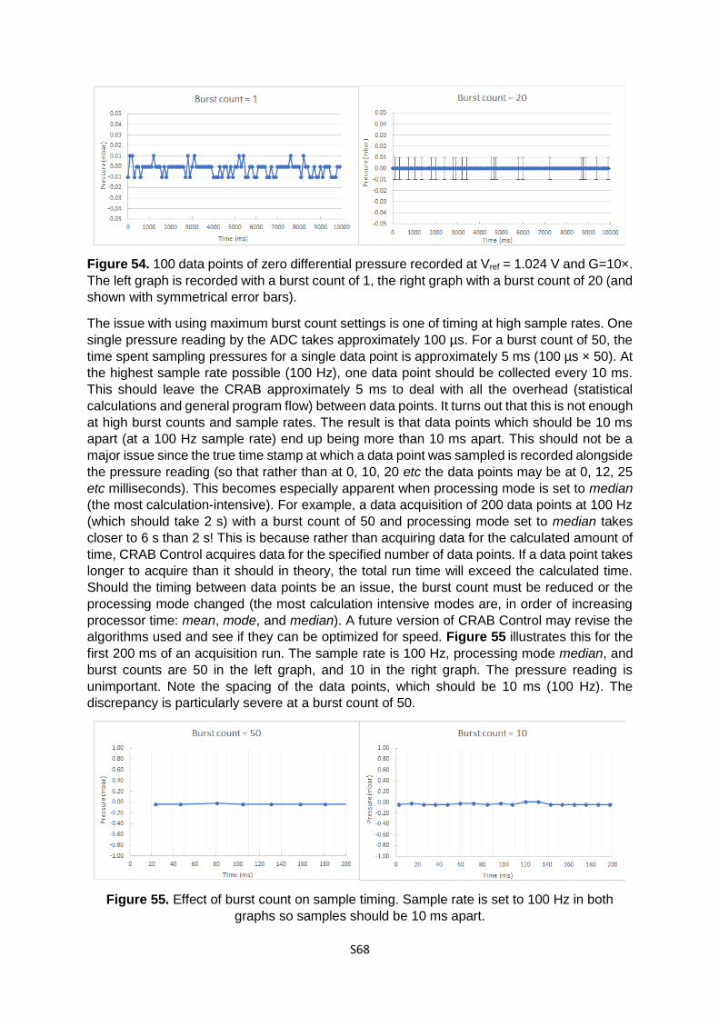
S68
Figure 54. 100 data points of zero differential pressure recorded at Vref = 1.024 V and G=10×.
The left graph is recorded with a burst count of 1, the right graph with a burst count of 20 (and
shown with symmetrical error bars).
The issue with using maximum burst count settings is one of timing at high sample rates. One
single pressure reading by the ADC takes approximately 100 µs. For a burst count of 50, the
time spent sampling pressures for a single data point is approximately 5 ms (100 µs × 50). At
the highest sample rate possible (100 Hz), one data point should be collected every 10 ms.
This should leave the CRAB approximately 5 ms to deal with all the overhead (statistical
calculations and general program flow) between data points. It turns out that this is not enough
at high burst counts and sample rates. The result is that data points which should be 10 ms
apart (at a 100 Hz sample rate) end up being more than 10 ms apart. This should not be a
major issue since the true time stamp at which a data point was sampled is recorded alongside
the pressure reading (so that rather than at 0, 10, 20 etc the data points may be at 0, 12, 25
etc milliseconds). This becomes especially apparent when processing mode is set to median
(the most calculation-intensive). For example, a data acquisition of 200 data points at 100 Hz
(which should take 2 s) with a burst count of 50 and processing mode set to median takes
closer to 6 s than 2 s! This is because rather than acquiring data for the calculated amount of
time, CRAB Control acquires data for the specified number of data points. If a data point takes
longer to acquire than it should in theory, the total run time will exceed the calculated time.
Should the timing between data points be an issue, the burst count must be reduced or the
processing mode changed (the most calculation intensive modes are, in order of increasing
processor time: mean, mode, and median). A future version of CRAB Control may revise the
algorithms used and see if they can be optimized for speed. Figure 55 illustrates this for the
first 200 ms of an acquisition run. The sample rate is 100 Hz, processing mode median, and
burst counts are 50 in the left graph, and 10 in the right graph. The pressure reading is
unimportant. Note the spacing of the data points, which should be 10 ms (100 Hz). The
discrepancy is particularly severe at a burst count of 50.
Figure 55. Effect of burst count on sample timing. Sample rate is set to 100 Hz in both
graphs so samples should be 10 ms apart.
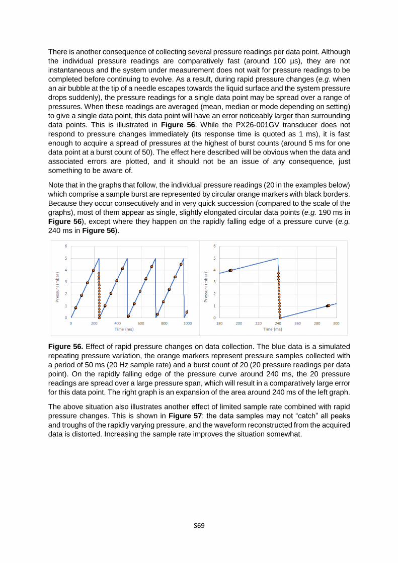
S69
There is another consequence of collecting several pressure readings per data point. Although
the individual pressure readings are comparatively fast (around 100 µs), they are not
instantaneous and the system under measurement does not wait for pressure readings to be
completed before continuing to evolve. As a result, during rapid pressure changes (e.g. when
an air bubble at the tip of a needle escapes towards the liquid surface and the system pressure
drops suddenly), the pressure readings for a single data point may be spread over a range of
pressures. When these readings are averaged (mean, median or mode depending on setting)
to give a single data point, this data point will have an error noticeably larger than surrounding
data points. This is illustrated in Figure 56. While the PX26-001GV transducer does not
respond to pressure changes immediately (its response time is quoted as 1 ms), it is fast
enough to acquire a spread of pressures at the highest of burst counts (around 5 ms for one
data point at a burst count of 50). The effect here described will be obvious when the data and
associated errors are plotted, and it should not be an issue of any consequence, just
something to be aware of.
Note that in the graphs that follow, the individual pressure readings (20 in the examples below)
which comprise a sample burst are represented by circular orange markers with black borders.
Because they occur consecutively and in very quick succession (compared to the scale of the
graphs), most of them appear as single, slightly elongated circular data points (e.g. 190 ms in
Figure 56), except where they happen on the rapidly falling edge of a pressure curve (e.g.
240 ms in Figure 56).
Figure 56. Effect of rapid pressure changes on data collection. The blue data is a simulated
repeating pressure variation, the orange markers represent pressure samples collected with
a period of 50 ms (20 Hz sample rate) and a burst count of 20 (20 pressure readings per data
point). On the rapidly falling edge of the pressure curve around 240 ms, the 20 pressure
readings are spread over a large pressure span, which will result in a comparatively large error
for this data point. The right graph is an expansion of the area around 240 ms of the left graph.
The above situation also illustrates another effect of limited sample rate combined with rapid
pressure changes. This is shown in Figure 57: the data samples may not “catch” all peaks
and troughs of the rapidly varying pressure, and the waveform reconstructed from the acquired
data is distorted. Increasing the sample rate improves the situation somewhat.
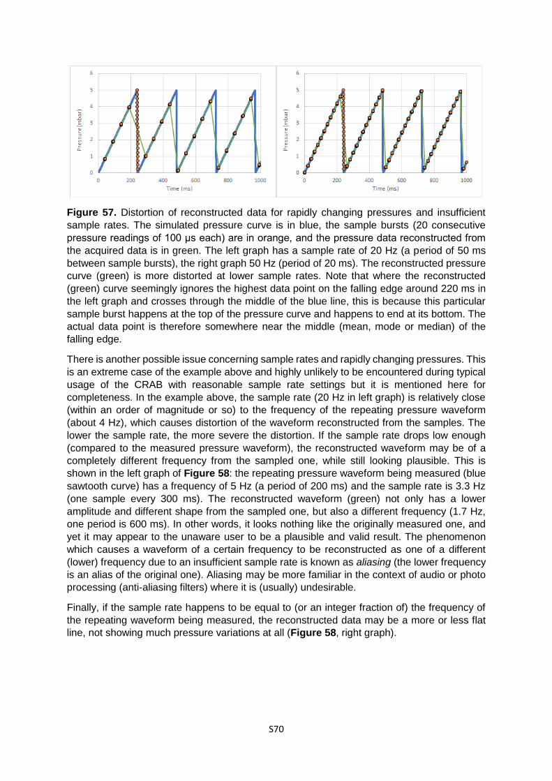
S70
Figure 57. Distortion of reconstructed data for rapidly changing pressures and insufficient
sample rates. The simulated pressure curve is in blue, the sample bursts (20 consecutive
pressure readings of 100 μs each) are in orange, and the pressure data reconstructed from
the acquired data is in green. The left graph has a sample rate of 20 Hz (a period of 50 ms
between sample bursts), the right graph 50 Hz (period of 20 ms). The reconstructed pressure
curve (green) is more distorted at lower sample rates. Note that where the reconstructed
(green) curve seemingly ignores the highest data point on the falling edge around 220 ms in
the left graph and crosses through the middle of the blue line, this is because this particular
sample burst happens at the top of the pressure curve and happens to end at its bottom. The
actual data point is therefore somewhere near the middle (mean, mode or median) of the
falling edge.
There is another possible issue concerning sample rates and rapidly changing pressures. This
is an extreme case of the example above and highly unlikely to be encountered during typical
usage of the CRAB with reasonable sample rate settings but it is mentioned here for
completeness. In the example above, the sample rate (20 Hz in left graph) is relatively close
(within an order of magnitude or so) to the frequency of the repeating pressure waveform
(about 4 Hz), which causes distortion of the waveform reconstructed from the samples. The
lower the sample rate, the more severe the distortion. If the sample rate drops low enough
(compared to the measured pressure waveform), the reconstructed waveform may be of a
completely different frequency from the sampled one, while still looking plausible. This is
shown in the left graph of Figure 58: the repeating pressure waveform being measured (blue
sawtooth curve) has a frequency of 5 Hz (a period of 200 ms) and the sample rate is 3.3 Hz
(one sample every 300 ms). The reconstructed waveform (green) not only has a lower
amplitude and different shape from the sampled one, but also a different frequency (1.7 Hz,
one period is 600 ms). In other words, it looks nothing like the originally measured one, and
yet it may appear to the unaware user to be a plausible and valid result. The phenomenon
which causes a waveform of a certain frequency to be reconstructed as one of a different
(lower) frequency due to an insufficient sample rate is known as aliasing (the lower frequency
is an alias of the original one). Aliasing may be more familiar in the context of audio or photo
processing (anti-aliasing filters) where it is (usually) undesirable.
Finally, if the sample rate happens to be equal to (or an integer fraction of) the frequency of
the repeating waveform being measured, the reconstructed data may be a more or less flat
line, not showing much pressure variations at all (Figure 58, right graph).
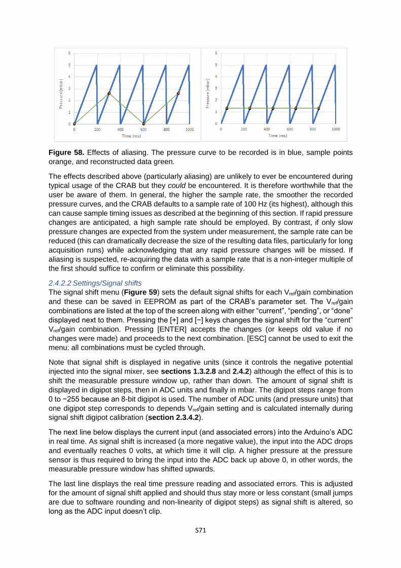
S71
Figure 58. Effects of aliasing. The pressure curve to be recorded is in blue, sample points
orange, and reconstructed data green.
The effects described above (particularly aliasing) are unlikely to ever be encountered during
typical usage of the CRAB but they could be encountered. It is therefore worthwhile that the
user be aware of them. In general, the higher the sample rate, the smoother the recorded
pressure curves, and the CRAB defaults to a sample rate of 100 Hz (its highest), although this
can cause sample timing issues as described at the beginning of this section. If rapid pressure
changes are anticipated, a high sample rate should be employed. By contrast, if only slow
pressure changes are expected from the system under measurement, the sample rate can be
reduced (this can dramatically decrease the size of the resulting data files, particularly for long
acquisition runs) while acknowledging that any rapid pressure changes will be missed. If
aliasing is suspected, re-acquiring the data with a sample rate that is a non-integer multiple of
the first should suffice to confirm or eliminate this possibility.
2.4.2.2 Settings/Signal shifts
The signal shift menu (Figure 59) sets the default signal shifts for each Vref/gain combination
and these can be saved in EEPROM as part of the CRAB’s parameter set. The Vref/gain
combinations are listed at the top of the screen along with either “current”, “pending”, or “done”
displayed next to them. Pressing the [+] and [−] keys changes the signal shift for the “current”
Vref/gain combination. Pressing [ENTER] accepts the changes (or keeps old value if no
changes were made) and proceeds to the next combination. [ESC] cannot be used to exit the
menu: all combinations must be cycled through.
Note that signal shift is displayed in negative units (since it controls the negative potential
injected into the signal mixer, see sections 1.3.2.8 and 2.4.2) although the effect of this is to
shift the measurable pressure window up, rather than down. The amount of signal shift is
displayed in digipot steps, then in ADC units and finally in mbar. The digipot steps range from
0 to −255 because an 8-bit digipot is used. The number of ADC units (and pressure units) that
one digipot step corresponds to depends Vref/gain setting and is calculated internally during
signal shift digipot calibration (section 2.3.4.2).
The next line below displays the current input (and associated errors) into the Arduino’s ADC
in real time. As signal shift is increased (a more negative value), the input into the ADC drops
and eventually reaches 0 volts, at which time it will clip. A higher pressure at the pressure
sensor is thus required to bring the input into the ADC back up above 0, in other words, the
measurable pressure window has shifted upwards.
The last line displays the real time pressure reading and associated errors. This is adjusted
for the amount of signal shift applied and should thus stay more or less constant (small jumps
are due to software rounding and non-linearity of digipot steps) as signal shift is altered, so
long as the ADC input doesn’t clip.

S72
Figure 59. The Settings/Signal shifts screen.
2.4.2.3 Settings/Load settings
This allows recalling of a parameter set from EEPROM (see section 2.3.3 and Figure 42). All
working memory parameters changed but not saved will be overwritten by the parameter set
from EEPROM. The saved parameter set is loaded from EEPROM when the CRAB is power
cycled or reset, but only after a key press from the user at the initial welcome message.
Adjustment of the trimpots VR1 and VR2 during the commissioning stage of the CRAB can be
carried out while the welcome message is displayed and before the user presses any
keyboard keys (see section 2.2.2).
Figure 60. Screen after loading settings from EEPROM.
2.4.2.4 Settings/Save settings
This saves the entire current parameter set (section 2.3.3 and Figure 42). Any previous
parameter set in EEPROM will be overwritten. The current version of CRAB Control only
allows one parameter set in EEPROM, a future version of CRAB Control may allow more than
one to be stored.
Figure 61. Press [Y] to store current parameter set in EEPROM.
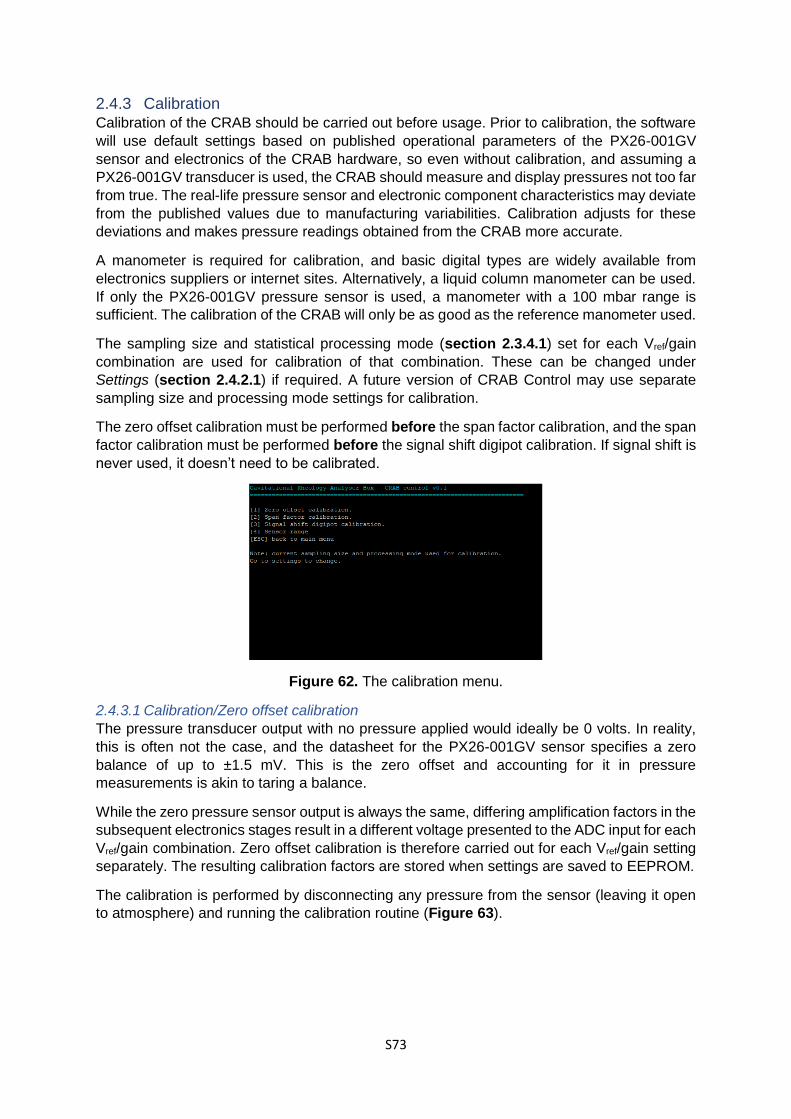
S73
2.4.3 Calibration Calibration of the CRAB should be carried out before usage. Prior to calibration, the software
will use default settings based on published operational parameters of the PX26-001GV
sensor and electronics of the CRAB hardware, so even without calibration, and assuming a
PX26-001GV transducer is used, the CRAB should measure and display pressures not too far
from true. The real-life pressure sensor and electronic component characteristics may deviate
from the published values due to manufacturing variabilities. Calibration adjusts for these
deviations and makes pressure readings obtained from the CRAB more accurate.
A manometer is required for calibration, and basic digital types are widely available from
electronics suppliers or internet sites. Alternatively, a liquid column manometer can be used.
If only the PX26-001GV pressure sensor is used, a manometer with a 100 mbar range is
sufficient. The calibration of the CRAB will only be as good as the reference manometer used.
The sampling size and statistical processing mode (section 2.3.4.1) set for each Vref/gain
combination are used for calibration of that combination. These can be changed under
Settings (section 2.4.2.1) if required. A future version of CRAB Control may use separate
sampling size and processing mode settings for calibration.
The zero offset calibration must be performed before the span factor calibration, and the span
factor calibration must be performed before the signal shift digipot calibration. If signal shift is
never used, it doesn’t need to be calibrated.
Figure 62. The calibration menu.
2.4.3.1 Calibration/Zero offset calibration
The pressure transducer output with no pressure applied would ideally be 0 volts. In reality,
this is often not the case, and the datasheet for the PX26-001GV sensor specifies a zero
balance of up to ±1.5 mV. This is the zero offset and accounting for it in pressure
measurements is akin to taring a balance.
While the zero pressure sensor output is always the same, differing amplification factors in the
subsequent electronics stages result in a different voltage presented to the ADC input for each
Vref/gain combination. Zero offset calibration is therefore carried out for each Vref/gain setting
separately. The resulting calibration factors are stored when settings are saved to EEPROM.
The calibration is performed by disconnecting any pressure from the sensor (leaving it open
to atmosphere) and running the calibration routine (Figure 63).
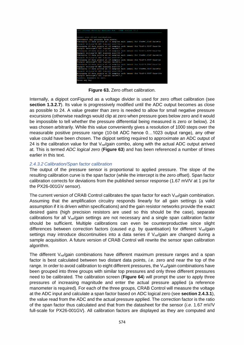
S74
Figure 63. Zero offset calibration.
Internally, a digipot conFigured as a voltage divider is used for zero offset calibration (see
section 1.3.2.7). Its value is progressively modified until the ADC output becomes as close
as possible to 24. A value greater than zero is needed to allow for small negative pressure
excursions (otherwise readings would clip at zero when pressure goes below zero and it would
be impossible to tell whether the pressure differential being measured is zero or below). 24
was chosen arbitrarily. While this value conveniently gives a resolution of 1000 steps over the
measurable positive pressure range (10-bit ADC hence 0…1023 output range), any other
value could have been chosen. The digipot setting required to approximate an ADC output of
24 is the calibration value for that Vref/gain combo, along with the actual ADC output arrived
at. This is termed ADC logical zero (Figure 63) and has been referenced a number of times
earlier in this text.
2.4.3.2 Calibration/Span factor calibration
The output of the pressure sensor is proportional to applied pressure. The slope of the
resulting calibration curve is the span factor (while the intercept is the zero offset). Span factor
calibration corrects for deviations from the published sensor response (1.67 mV/V at 1 psi for
the PX26-001GV sensor).
The current version of CRAB Control calibrates the span factor for each Vref/gain combination.
Assuming that the amplification circuitry responds linearly for all gain settings (a valid
assumption if it is driven within specifications) and the gain resistor networks provide the exact
desired gains (high precision resistors are used so this should be the case), separate
calibrations for all Vref/gain settings are not necessary and a single span calibration factor
should be sufficient. Multiple calibrations can even be counterproductive since slight
differences between correction factors (caused e.g. by quantisation) for different Vref/gain
settings may introduce discontinuities into a data series if Vref/gain are changed during a
sample acquisition. A future version of CRAB Control will rewrite the sensor span calibration
algorithm.
The different Vref/gain combinations have different maximum pressure ranges and a span
factor is best calculated between two distant data points, i.e. zero and near the top of the
range. In order to avoid calibration to eight different pressures, the Vref/gain combinations have
been grouped into three groups with similar top pressures and only three different pressures
need to be calibrated. The calibration screen (Figure 64) will prompt the user to apply three
pressures of increasing magnitude and enter the actual pressure applied (a reference
manometer is required). For each of the three groups, CRAB Control will measure the voltage
at the ADC input and calculate a span factor based on ADC logical zero (see section 2.4.3.1),
the value read from the ADC and the actual pressure applied. The correction factor is the ratio
of the span factor thus calculated and that from the datasheet for the sensor (i.e. 1.67 mV/V
full-scale for PX26-001GV). All calibration factors are displayed as they are computed and

S75
should be both close to 1.00 and close (ideally equal) to each other. If all calibration factors
are similar but very different from 1.00, it may be that a sensor different from the PX26-001GV
is being used but CRAB Control has not been told (see section 2.4.3.4), or that the sensor is
defective. If only some of the calibration factors are very different from 1.00 (but the others are
similar to each other and close to 1.00), then this may indicate a fault with the Vref and/or gain
circuitry of the CRAB. The span correction factors are saved in EEPROM along with all other
settings.
Figure 64. Span factor calibration.
2.4.3.3 Calibration/Signal shift digipot calibration
The signal shifter uses a digipot to lower the voltage reaching the Arduino’s ADC, thus moving
the measurable pressure window upwards. The theoretical amount of voltage shift per digipot
step for each Vref/gain combination can be calculated from other parameters in the circuit, and
these are the default values used before calibration. Due to manufacturing variabilities, it is
preferable to measure the actual amount of shift per step. CRAB Control does this by
measuring the ADC input at a given test pressure, then increasing the amount of shift applied
in steps until the measured ADC input is at or close to logical zero (see section 2.4.3.1). The
amount of shift (in ADC units per step) is calculated from the difference in initial and final ADC
reading and number of digipot steps applied.
Similar to span factor calibration, the user is asked to apply a number of increasing test
pressures to the CRAB, which then carries out the process described above. Similar to span
factor calibration, separate calibrations for each Vref/gain settings should not be necessary and
the signal shift calibration routine may be rewritten in a future version of CRAB Control.
Figure 65. Signal shift digipot calibration.
2.4.3.4 Calibration/Sensor range
This feature was added when it was realised that pressure transducers other than the PX26-
001GV would need to be used with the CRAB. It simply tells CRAB Control the output voltage
of the transducer at full rated pressure. These two parameters are used in all other pressure

S76
calculations by CRAB Control. The CRAB can thus be adapted, within limits, to work with
pressure transducers other than the PX26-001GV.
Since the circuitry of the CRAB was designed around the PX26-001GV sensor, other sensors
may only be usable through part of their range with clipping at the ADC input occurring and
unexpectedly limiting the measurable pressure range.
Figure 66. Sensor range calibration.
2.4.4 Remote operation This is intended to initiate communication with client software on a computer and will be
implemented in a future version of CRAB Control.
2.4.5 Info This gives software and hardware version and author information.
Figure 67. The info screen.