HEDG Working Paper 07/24

Using copulas to measure association between ordinal measures of health and income

Casey Quinn

October 2007

ISSN 1751-1976

york.ac.uk/res/herc/hedgwp

Using copulas to measure association between

ordinal measures of health and income

Casey Quinn

University of York, York YO10 5DD, England

Lehigh University, Bethlehem, PA 18015, USA

October 22, 2007

Abstract

This paper introduces a new approach to measuring the association between

health and socioeconomic status. Measuring inequalities in health is difficult

when health is measured qualitatively, specifically on an ordinal scale. This

paper demonstrates a rank-based dependence measure - the copula - that is

invariant to both the scale and any monotonic transformations of its dimensions.

Accordingly, the copula measure of association between health and income is

robust under different cardinal scales for health as well as different income

distributions, and can be used for ordering countries. The copula is also used

to generate contingency tables of joint probability, which illustrate how this

ordering can be due to polarity in the distributions of health and income, as

well as stronger association between the distributions of health and income.

1

1 Introduction

In this paper I consider income-related inequalities in health across 4 countries within

the European Community Household Panel (ECHP) survey: the United Kingdom,

Germany, Greece and Portugal. Income is measured, in all 4 countries, in various

forms, leading ultimately to a measure of post-tax household equivalised income, ad-

justed for Purchasing Power Parity (PPP) across the countries. For most comparisons

(e.g. considering income inequality) this is not problematic. What is problematic is

the measurement of Self-Assessed Health (SAH) on an ordinal scale - typically "Very

Good", "Good", "Fair", "Poor" and "Very Poor". As is demonstrated elsewhere

(see for example Allison and Foster 2004, and Zheng 2006), the distribution of the

responses on this scale - referring to their subsequent cardinal values - becomes dif-

ferent depending upon the cardinal scale to which it is transformed. In particular,

mean-based measures of inequality (or, in multiple dimensions, covariance) are not

robust under some such transformations.

This analysis is, by design, straightforward, relative to the broader considera-

tion of health inequalities. Inequalities in health are not considered explicitly, while

income-related inequalities in health are defined according to, for example, Wagstaff

and van Doorslaer (2000). In Wagstaff, et al.’s (1991) paper, the authors asked the

question, "To what extent are there inequalities in health that are systematically

related to socioeconomic status?". Similarly, the International Society for Equity

in Health (ISEqH, 2001) defined this as equity, specifically: "...the absence of po-

tentially remediable, systematic differences in one or more aspects of health across

socially, economically, demographically or geographically defined population groups

or subgroups."

Bommier and Stecklov (2002) consider an extra-welfarist definition, stating that an

ideal equitable society was one in which access to health, rather than health itself, was

not determined by socioeconomic status or income, according to Rawlsian principles

2

of justice. The analysis here follows the former definitions. This assumes that, for

empirical purposes, health outcomes (SAH specifically) can be used to consider the

distribution of health, and how it is related to the distribution of income.1

According to such definitions, health inequality of a socioeconomic nature can be

defined by its absence: a perfectly ’fair’ distribution of health contains an absence of

association between socioeconomic status and health, or between the distribution of

income and the distribution of health. This is the one considered in the construction

of the concentration curve and index (Wagstaff, et al. 1991; Kakwani, et al. 1997).

In their measure of inequality, the covariance between health status and the rank

of individual income in the income distribution is used. The meaning is the same:

higher values of the concentration index result from stronger covariance, i.e. stronger

association between health and income. Returning to Bommier and Stecklov (2002),

however, the optimal measure of socioeconomic inequalities in health is one that

can measure the association between the distributions of health and income without

influence from the distributions themselves (i.e. invariant to the cardinal scale given

to SAH, and invariant to any inequality in the distribution only of income).

The method used in this paper - the copula - is a rank-based measure of as-

sociation between monotonic transformations of random variables rather than the

variables themselves: i.e. a bivariate distribution of univariate distribution functions.

Specifically, this paper takes advantage of the functional relationship between the

Archimedean class of copulas and measures of rank correlation to demonstrate that

the health and income distributions of different countries can be ordered according to

principles of stochastic dominance. This ordering is robust under both the discrete

nature of SAH and transformations of the cardinal scale(s) applied to SAH. Following

work by Contoyannis and Wildman (2006), the copula for each country shows that,

for example, Greece exhibits inequality in more of the bivariate distribution of health

and income, however Portugal exhibits greater polarity between low health and high

income, resulting in Greece dominating Portugal in terms of association between the

3

distributions of health and income.

2 Measuring ordinal health and health inequality

Ordinal measurement of SAH is known to be problematic for the analysis of health.

As an ordinal measure of health, SAH also suffers by comparison to continuous mea-

sures of welfare. As a categorical measure, SAH is not necessarily Lorenz consistent;

according to the Pigou-Dalton transfer principle that progressive transfers reduce in-

equality and/or make society better-off (Chateauneuf and Moyes 2005; Zheng 2006).

First and foremost is the practical consideration: ’health’ itself is not transferable.

Secondly, a progressive transfer in ordinal scale does not necessarily mean a transfer

across cut-points. A transfer of health from a person with very Very Good health to

a person who only just has Very Good health will not alter any measure of health

inequality, irrespective of the cardinal scale to which SAH is adapted.

In terms of the first consideration, some authors recommend measuring inequality

still within the framework of progressive transfers, but such that non-transferable

dimensions of the social welfare function - progressive or otherwise - be left out of

the measure (Bosmans, et al. 2006). Bommier and Stecklov (2002) discuss this also

with respect to Rawlsian principles of justice: health itself should not be considered

a basic freedom, deserving of equal distribution, but access to health or health care

should, similar to Sen’s (1979) equality of opportunity (Rosa Dias and Jones 2007).

Retaining health in the measurement of welfare and inequality means addressing

the nature of common health measures, as well as defining how inequality in health

is to be considered: for example access to health care versus its utilisation versus

its outcomes (Braveman 2006). One such measure is the concentration index, which

considers the association an individual’s health and the rank of their income.

4

2.1 Concentration curves and indices with discrete SAH

The concentration curve was defined in Kakwani (1977) as representing the rela-

tionship between the distribution function F (y) - where y is given to be income,

for example, and some other monotonic function F1 (y), or in the case of Kakwani’s

(1977) demonstration, F1 (g(y)) . Kakwani (1977) in particular identified g(y) and

F1 (g(y)) such that the Lorenz curve is seen as a special form of the concentration

curve - what he called a relative concentration curve.2

The concentration curve, as it is known to health economists, is one represent-

ing the relationship between functions of two related variables, rather than a single

variable. I.e., individuals are ranked according to income, for example, while we are

interested in their cumulative share of health (rather than ranking them according

to income and being interested in each rank’s cumulative share of income, also).

Wagstaff, et al. (1991) present their generalised concentration curve relating the

cumulative amount of health to the rank of individuals according to socioeconomic

status, their interest being in the socioeconomic dimension of inequalities in health.3

The concentration curve was similarly employed with mortality, previously (Preston,

et al. 1981; Leclerc, et al. 1990).

Interpretation of the concentration curve is the same as for the Lorenz curve: the

45◦ line represents perfect (socioeconomic) equality in health. A curve observed above

this diagonal at all points represents pro-poor inequality, while one below represents

pro-rich inequality. For the purposes of comparison the same principle applies to the

concentration curve. For two random variables Y1 and Y2 representing the incomes

in country 1 and country 2, respectively, and with the same ranking function F (.),

their concentration curves C1 and C2 will be the cumulative share of health in each

country, G(.). Thus C1 will Lorenz dominate (i.e. be at all points above) C2 iff

C1 ≥ C2 ∀ F (y1) or F (y2). That is, for all ranks of income, the concentration curve of

country 1 must be strictly no less than that of country 2. Dominance does not occur

5

when the lines cross. Since this is more commonly observed, the concentration index

is employed instead as the measure of relative (in)equality (see Hernández Quevedo,

et al. 2006 for their comparison of all ECHP countries).

The concentration index is used as a numerical measure of distance between the

observed concentration curve and the line of equality - twice the area, like the Gini

coefficient. It can therefore be used to compare two or more overlapping concentration

curves, establishing generalised Lorenz dominance of one country over another.

There are several representations of the concentration index; the most useful for

this analysis is the ’convenient covariance’ representation, in which each individual’s

health hi (from a distribution with mean μh) is indexed against their rank Ri in the

distribution of income Y (Kakwani 1980; Wagstaff, et al. 2003). Thus

CI =2

μh (n− 1)nPi=1

(hi − μh)

µRi −

1

2

¶(1)

=2

μhcov (hi, Ri)

for a sample size n. The concentration index is the scaled covariance between

the health of the individual and their rank in the income distribution. Thus income-

related inequality in health is this measure of covariance such that CI = 0 when there

is no inequality - i.e. there is no observed association between socioeconomic status

and health - and −1 ≤ CI ≤ 1 due to the 2μhterm.4 This association, or lack thereof,

forms the basis of the measurement of socioeconomic-related inequalities in health,

according to the criteria of Wagstaff, et al. (1991) and Bommier and Stecklov (2002),

among others.

As a measure of covariance, the concentration index relies upon the means of the

distributions of health and income

6

CI =2

μhcov (h,R) (2)

=2

μhcov (h, F (y))

=2

μh[E (h, F (y))−E (h)E (F (y))]

Reliance on the mean is problematic in the case of the distribution of health,

which is typically measured on an ordinal scale, rather than a cardinal one. Allison

and Foster (2004), for example, demonstrate that the mean of a cardinal scale is not

a robust measure of ordinal-scale health. They employ different cardinal scales, from

linear to highly concave, for the ordinal SAH scale c = [1, 2, 3, 4, 5]. They show that

inequality rankings can be reversed by using different cardinal scales - i.e. different

relative values of health. This is also shown to be the case with first-order dominance,

when the mean is used to normalise the measure of inequality, as it is in Equations

(1) and (2). In the case of the concentration index, using covariance has a similar

effect: as long as the function Ri is used to rank income, non-linear transformations

of income will have no effect (e.g. a change in the tax schedule), but those of health

will. A linear cardinal scale will provide a different measure of linear covariance

than a highly concave one, for example. The implication of this for concentration

index-based ordering of countries is demonstrated in Tables 4.1 and 4.2.

2.2 Transforming SAH so that it is continuous

SAH has been rendered continuous in the past by inverting a covariate-dependent

distribution function F (h∗). Procedurally, this involves using, for example, an or-

dered probit model of latent health h∗ = X 0β+ ε. The regression link between latent

health h∗ and assessed health h is given by the ordered probit, such that h = j if

μj−1 < X 0β ≤ μj for j = 1, .., 5 (van Doorslaer and Jones 2003), where unobserved

7

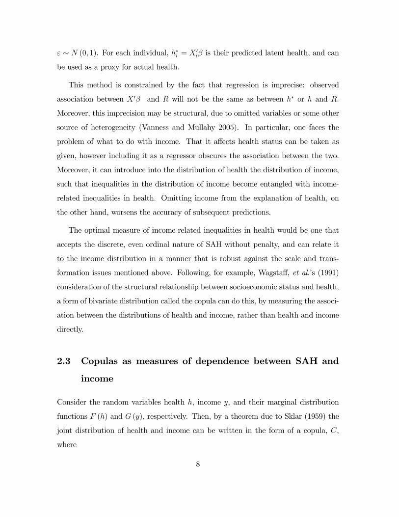
ε ∼ N (0, 1). For each individual, h∗i = X 0iβ is their predicted latent health, and can

be used as a proxy for actual health.

This method is constrained by the fact that regression is imprecise: observed

association between X 0β and R will not be the same as between h∗ or h and R.

Moreover, this imprecision may be structural, due to omitted variables or some other

source of heterogeneity (Vanness and Mullahy 2005). In particular, one faces the

problem of what to do with income. That it affects health status can be taken as

given, however including it as a regressor obscures the association between the two.

Moreover, it can introduce into the distribution of health the distribution of income,

such that inequalities in the distribution of income become entangled with income-

related inequalities in health. Omitting income from the explanation of health, on

the other hand, worsens the accuracy of subsequent predictions.

The optimal measure of income-related inequalities in health would be one that

accepts the discrete, even ordinal nature of SAH without penalty, and can relate it

to the income distribution in a manner that is robust against the scale and trans-

formation issues mentioned above. Following, for example, Wagstaff, et al.’s (1991)

consideration of the structural relationship between socioeconomic status and health,

a form of bivariate distribution called the copula can do this, by measuring the associ-

ation between the distributions of health and income, rather than health and income

directly.

2.3 Copulas as measures of dependence between SAH and

income

Consider the random variables health h, income y, and their marginal distribution

functions F (h) and G (y), respectively. Then, by a theorem due to Sklar (1959) the

joint distribution of health and income can be written in the form of a copula, C,

where

8

H (h, y) = C (F (h) , G (y)) (3)

i.e. the copula is a multivariate distribution function not of random variables, but

the distribution functions of those random variables: a multivariate distribution with

strictly uniform margins. The copula is a function that parameterises the dependence

between univariate marginal distributions (in this case F (h) and G (y)) and binds

them to form the joint distribution function (given by C (F (h) , G (y))).

Copulas use measures of association that are invariant to monotonic - but not

necessarily strict or linear - transformations of random variables. Ergo unlike, for

example, the bivariate normal distribution, the association between h and y is the

same as between F (h) and G(y). The rank correlations of Kendall and Spearman

are familiar examples of such measures of association. Like the bivariate normal, any

bivariate copula is an approximation to the true bivariate distribution H; except with

the advantage that the marginal distributions are, by construction, tractable: they

are free of every other marginal distribution in the joint distribution, and separated

also from the measure of association.

There are many families of copulas (see Joe 1997; Nelsen 2006). Here I use a spe-

cific class known as the Archimedean copula. This class is distinguishable by the fact

that its measure of association, θ, is functionally related to rank correlation. Specifi-

cally, for any copula C with continuous univariate margins u|u=F (h) and v|v=G(y), the

copula C (u, v; θ) is such that (Nelsen 2006)

Kendall’s τ = 4Z Z

I2C (u, v) dC (u, v)− 1 (4)

and

Spearman’s ρ = 12Z Z

I2C (u, v) dudv − 3 (5)

where I2 refers to the bivariate uniform (0, 1)2 space. Archimedean copulas in

particular are constructed by so-called generator functions such that

9

C (u, v) = ϕ−1 (ϕ (u) + ϕ (v)) (6)

where the generator ϕ (.) is unique to each copula (see Nelsen 2006).

The differences between Spearman’s ρ and Kendall’s τ are discussed in Nelsen

(2006) and Fredericks and Nelsen (2007). For absolutely continuous distributions u

and v the use of either is equivalent. No general guideline exists, suggesting which

circumstances are preferred for one method or another.5 For applied research purposes

the use of Kendall’s τ can be more convenient as the functional form of the relationship

with the copula parameter θ is available (Genest and Rivest 1993; Nelsen 2006). As

discussed below, the use of SAH makes Kendall’s τ a preferred reference for the

Genest-Rivest solutions for estimating θ.

For each Archimedean copula, Kendall’s τ can be given by

τ = 4

Z ZI2C(u, v)dC(u, v)− 1 (7)

= 1 + 4

Z 1

0

ϕ (t)

ϕ0 (t)dt

For some marginal distribution t. Then in sample space for health and income

(h, y)

τ =³n2

´−1Xi<j

sign [(hi − hj) (yi − yj)] (8)

Solving Equations (7, 8) for τ = τ and a given Archimedean generator function

ϕ(t) will provide a sample estimate of θ (Genest and Rivest 1993).

The complexity of Equations (4 - 8) belies the simplicity of this approach in prac-

tice, and particularly when analysing SAH, due to its distribution being discrete, i.e.

10

not a strictly-increasing function of the random variable SAH. For the representa-

tions in Equations (4) and (5) to hold strictly, τ must be an increasing function of

the association parameter θ.

That SAH is distributed discretely while income is continuous is not problematic:

the margins of a copula can be mixed, so that non-parametric analysis can used;

the histogram of SAH can be used with the continuous empirical or kernel distrib-

ution of income. Because of the functional relationship between θ and τ , Kendall’s

so-called tau-b (hereafter denoted τ b) can be used to estimate θ, following Vanden-

hende and Lambert (2000, 2003), which can be combined to calculate joint probabil-

ities.Kendall’s τ b is one of two generalisation for ordinal data with ties. For a square

contingency table with C concordant pairs, D discordant pairs and non-tied pairs on

the vectors of health or income (Oh and Oy respectively), τ b is given by

τ b =(C −D)q¡

C +D − Oh

¢ ¡C +D − Oy

¢ (9)

Vandenhende and Lambert (2000) analyse the extent of this problem; the degree

to which the copula τ in Equation (4) will not correspond to τ b. I.e. the degree

to which τ b may not be a strictly increasing function of the copula’s association

parameter θ. They found that the relationship was preserved in the case of the Frank

copula, which is positively ordered; they also observed monotonocity for non-ordered

copulas when dependence was not weak.6 The relationship between τ b and θ also

proved to be stronger as the number of categories in the margins increased. They

observed the margins to behave more like continuous margins, rather than discrete

as they increased categories from 4 to 10.7

Association θ can be estimated directly for each copula: Full-Information Maxi-

mum Likelihood (FIML), for example, was used by Cameron, et al. (2003; Kolesárová

and Mordelová 2006 also discuss this issue). However the discrete/continuous mixture

makes this more difficult to estimate directly. Cameron, et al. (2004) in particular

11

discuss the relative merits of this approach compared to FIML, using binary data.

Following Vandenhende and Lambert (2003), and considering that SAH is usually

measured in 5 categories, the indirect approach is preferable here.

The tractability of copulas means the copula of one country is directly comparable

to that of another country, allowing for countries to be ordered according to stochastic

dominance, similar though not entirely analogous to lorenz dominance. Finally, either

measure of association θ or τ can be used for rank dominance.

2.3.1 The Frank copula

The Frank copula is given by (Frank, 1979)

C (u, v; θ) = −1θln

Ã1 +

¡e−θu − 1

¢ ¡e−θv − 1

¢e−θ − 1

!(10)

where θ ∈ (−∞,∞) \ {0}. The Frank copula is constructed using the generator

function

ϕθ (t) = − lnµe−θt − 1e−θ − 1

¶(11)

This is a comprehensive family, such that association θ corresponds to τ ∈ [−1, 1] \

{0}.8 The tau link function for the Frank generator is given by

τ = 1− 4θ

∙1

θ

θR0

t

et − 1dt+θ − 22

¸(12)

2.3.2 The Gumbel copula

The Gumbel copula is a single-parameter distribution function, like the Frank.9 How-

ever, the Gumbel copula is skewed such that dependence is measured more precisely

in the upper tail than the lower (i.e. "high-high" combinations: see Figure 4.1; Trivedi

12

and Zimmer 2006). It is therefore suited in particularly not only to random variables

that are positively correlated, but to those in which high values of each are more

strongly correlated than low values.

The Gumbel copula is given by

C(u, v; θ) = exp

∙−h(− lnu)θ + (− ln v)θ

i 1θ

¸(13)

where θ ∈ [1,∞). The Gumbel copula is constructed using the generator function

ϕθ (t) = (− ln t)θ (14)

For which the tau link function is given by

τ = 1− θ−1 (15)

This corresponds to positive association only θ → τ ∈ [0, 1].

2.3.3 The AMH copula

The AMH copula is skewed in its dependence structure, similar to the Gumbel, how-

ever it estimates dependence more precisely in the lower tail (i.e. "low-low" combina-

tions, when dependence is positive: see Figure 4.1). It is suited to joint distributions

where positive correlation (in this case) is strongest between low values, relative to

high values, of the random variables.

The AMH copula is given by (Ali, et al. 1978)

C (u, v; θ) =uv

1− θ (1− u) (1− v)(16)

where θ ∈ [−1, 1) corresponds to τ ∈£−0.181726, 1

3

¤. The AMH copula is con-

structed using the generator function

13

ϕθ (t) = ln

µ1− θ (1− t)

t

¶(17)

For which the tau link function is given by

τ = 1 + 2

"−16θ−£(θ − 1)2 ln (1− θ)

¤3θ2

#(18)

Figure 4.1 contains an illustration of the distribution of simulated bivariate normal

data (ρ = 0.8). The only difference between the distributions is the copula used to

simulate the data: the margins are all standard-normally distributed, and they are

equally dependent, but the structure of that dependence is different for each. Greater

density of simulated data in the right tail of the Gumbel copula and the left tail of

the AMH copula reflect properties discussed above.

14

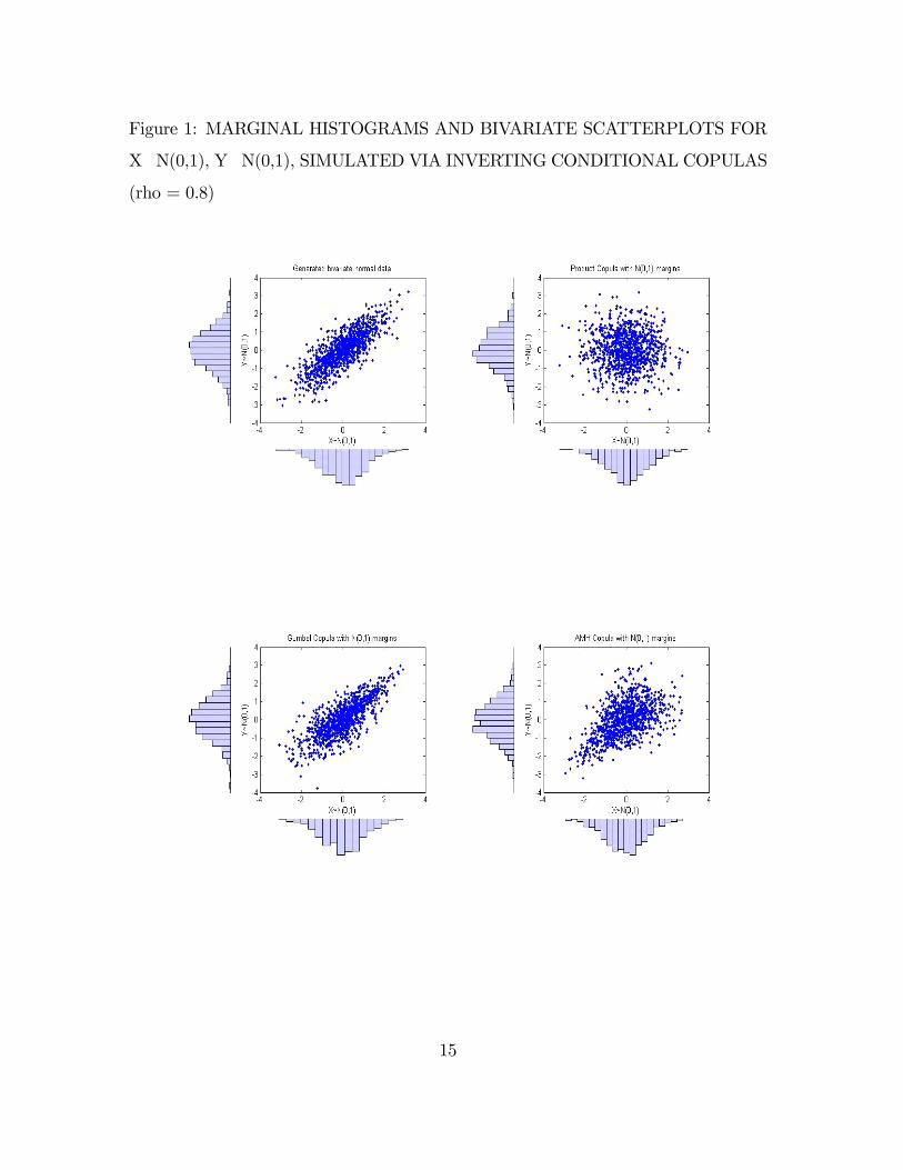
Figure 1: MARGINAL HISTOGRAMS AND BIVARIATE SCATTERPLOTS FOR

X N(0,1), Y N(0,1), SIMULATED VIA INVERTING CONDITIONAL COPULAS

(rho = 0.8)

15

MARGINALHISTOGRAMSANDBIVARIATE SCATTERPLOTS FORX N(0,1),

Y N(0,1), SIMULATED VIA INVERTING CONDITIONAL COPULAS (rho = 0.8)

16

The value of this is demonstrated later, when goodness-of-fit testing is employed

to determine which copula appears to be the better fit to the data. As well as

functionality as the bivariate distribution, this selection provides information about

the structure or shape of the dependence between random variables.

Solving Equations (12), (15) and (18) is possible using software such as Maple

or Mathematica, or with an implementable Matlab package (see Perkins and Lane

2003). Solutions for the estimates of Kendall’s τ b can be seen in Table 4.3.

Estimates of θ are necessary for each copula, but not for rank-ordering the coun-

tries according to their association between health and income. Association θ is, by

design, a monotonic function of τ : the rank-order of the countries will not change

because a different copula is used. What may change is the joint distribution as a

whole, due to the different shapes of copulas (see for example Joe, 1997; Bouyé, et

al. 2000).

3 Application: income-related inequalities in

health in the ECHP

3.1 Data

Data on SAH and income are drawn from the 7th wave (2000) of the European Com-

munity Household Panel Survey (ECHP: see Peracchi 2002 and Hernández Quevedo,

et al. 2006 for descriptions of the ECHP Users’ Database). Income in this data

is equivalised household income, adjusted for Purchasing Power Parity between the

countries.10 SAH is taken from responses to the question “How is your health in gen-

eral?” and contains 5 categorical responses: "Very Good", "Good", "Fair", "Poor"

and "Very Poor".11 Sample sizes ranged from 8,573 (the UK) to 11,035 (Portugal).

The 4 countries used were chosen for purposes of comparison with the UK. Looking

17

at inequalities in both health and income, Portugal has the greatest of both, Greece

has proximate inequalities in health (relative to the UK) but greater inequalities in

income, while Germany is among the countries with the lowest inequalities in each

- it sits on an interior frontier, along with Austria and Denmark (see for example

Jones and Rice 2004). Their respective distributions of SAH and income are shown

in Figures 4.2 and 4.3.

18

Figure 2: HISTOGRAMS FOR SELF-ASSESSED HEALTH IN THE UK, GER-

MANY, PORTUGAL AND GREECE

In distributional terms, SAH is roughly similar for all of the countries except

Greece, whose elevated self-assessment has been documented elsewhere (Cantarero

and Pascual 2005). The skewness in Greece’s SAH also generates a slightly higher

average health status than the UK, who would otherwise have the highest average

of the three less-skewed distributions. The distributions of equivalised household

income are also similar, although the UK and Germany have, predictably, higher

levels of household income. Portugal enjoys much less household income, relative to

the other three countries.

19

Figure 3: HISTOGRAMS FOR INCOME IN THE UK, GERMANY, PORTUGAL

AND GREECE

20

Table 1: CONCENTRATION INDICES AND MEAN HEALTH USING DIFFER-

ENT CARDINAL SCALES FOR HEALTH

3.2 Estimation

Estimation is undertaken according to the procedures described above. Methods for

estimating concentration curves and indices can be found in, for example, Wagstaff, et

al. (1991) and Wagstaff (2000). For the copulas, the procedure following Genest and

Rivest (1993) and Vandenhende and Lambert (2003) was employed: sample estimates

of Kendall’s τ c, shown in Table 4.1, were used to solve for θ in Matlab (see Perkins

and Lane, 2003). The copulas themselves were calculated in Stata, however they too

could have been calculated in Matlab.12

3.3 Results: concentration indices and curves

Following the example of Allison and Foster (2004), consider the concentration indices

CI of the UK, Portugal, Germany and Greece using CIUK , CIPortugal, CIGermany

and CIGreece and with health scales S1 = [1, 2, 3, 4, 5], S2 = [1, 2, 3, 4, 10], S3 =

[1, 2, 3, 4, 15] and S4 = [1, 4, 9, 16, 25] . The resulting indices from Equation (1) are

shown in Table 4.1, followed by the changes in index-based orderings of countries

shown in Table 4.2.

Any two (or more) non-degenerate distributions of discretely-identified health sta-

tus can be ordered differently according to different inequality indices or cardinal scale

(Zheng 2006; Allison and Foster 2004, respectively): any concentration index simi-

larly applied can be ordered differently depending upon the cardinal scale used, as

Tables 4.1 and 4.2 illustrate.

In Table 4.2, increasing the value or weight of only the highest health status

re-orders Portugal and Greece. Another increase in the value of the highest health

status subsequently re-orders Portugal and the UK, and so forth. Having the lower

21

Table 2: RANK-ORDERING USING DIFFERENT CARDINAL SCALES FOR

HEALTH

mean health, Portugal slowly moves up the order. Squaring the values relative to

the linear scale changes the values for the concentration indices, but not the order.

This re-ordering occurs despite relatively small absolute changes in the concentration

indices. The concentration curves under each cardinal scale of the UK, for example,

are nearly indistinguishable visually (see Figure 4.3).

22

Figure 5: CONCENTRATION CURVES FOR THE UK, GERMANY, PORTUGAL

AND GREECE, USING DIFFERENT CARDINAL SCALES FOR HEALTH

0

.2.4

.6.8

1H

ealth

0 .2 .4 .6 .8 1Income Rank

Scale 1: 1 to 5 Scale 2: 1 to 10Scale 3: 1 to 15 Scale 4: 1, 4,.., 25

Concentration Curves under varying cardinal scales for health

3.4 Results from copulas: rank-ordering and stochastic dom-

inance

Table 4.3 contains the estimates of the dependence parameter in each copula, following

the Genest-Rivest solutions shown above.

Having estimated rank-correlation τ b, using the work by Vandenhende and Lam-

bert (2000), changing the cardinal scale of health will not alter this estimate, or cause

any change in the estimates of the copula parameters, or in their ranking according

to association between the distributions of SAH and income. Testing is necessary,

23

Table 3: CONCENTRATION INDEX-ORDERS USING DIFFERENT CARDINAL

SCALES FOR HEALTH

Country bτ Frank Clayton AMH

UK 0.1318 1.2032 0.3036 0.5100 Portugal 0.1783 1.6475 0.4340 0.6529 Germany 0.0454 0.4093 0.0951 0.1941 Greece 0.1571 1.4429 0.3728 0.5900

however, to determine which copula is preferred.

3.4.1 Goodness of fit

Copulas can be compared according to goodness of fit in order to select the most ap-

propriate dependence structure, given the data. Following Fermanian (2005), a fairly

straightforward Chi-squared test-statistic comparing each copula (as a bivariate dis-

tribution function) to the bivariate standard uniform distribution can be calculated.

For well-fitting copulas, the hypothesis that the copula is not uniformly-distributed

should always be rejected, however the copula that fits the best should be rejected

the most strongly. Hence the highest of the Chi-squared test statistics will reveal the

best-fitting copula.

In this case the Gumbel copula is the best fit, for all countries, followed very

closely by the Frank copula. In fact the Frank copula’s Chi-squared statistic is not

significantly greater, in the statistical sense, than that of the Gumbel copula. Ac-

cording to the discussion preceding Figure 4.1, this indicates that the structure of

the dependence between health and income is generally symmetric about the centres

of the distributions, with slightly stronger dependence between high values of health

and income than low values.

24

3.4.2 Rank-ordering countries

The Gumbel copula has been retained hereon for comparison of the results.13 The

bivariate distribution function C³F (hi) , G (yi) ; θ

´for SAH status hi and income yi

can be calculated by using the estimates of dependence θ (based on τ b), as well as

histograms for SAH, F (h) and empirical CDFs for income, G (y). For the purposes

of determining stochastic dominance of one country over another, consider the joint

distributions of health and income for 2 countries, C1 (u1, v1) and C2 (u2, v2).

Following Dardanoni and Lambert (2001), the distribution of health and income in

country 1 is known according to C1 (u1, v1). It is to be compared to the distribution

of health and income in country 1 had it had the association of country 2. The

comparison will use the copula of country 2, containing the margins of country 1.

Then Country 1 ºI Country 2 ⇐⇒ C1 (u1, v1) ≥ C2 (u1, v1), i.e. if country 1 has a

stronger association between the distributions of health and income it has, according

to the definition here, more income-related inequality in health.

The counter-factual distribution can be manufactured with an exchange of copu-

las: for each country we can observe and estimate C1³u1, v1; θ1

´and C2

³u2, v2; θ2

´respectively, but then calculate C2

³u1, v1; θ2

´numerically. In fact the comparison is

more straightforward: C1 (u1, v1) ≥ C2 (u1, v1) iff C1 (u1, v1) ≥ C2 (u2, v2) as a result

of the transformations at the margins (Dardanoni and Lambert 2001). Only the cop-

ula for each country is needed for comparison. If the association between the health

and income is greater for one country than another, its copula will lie above that of

the other country and, as above, it has more income-related inequality in health.

The results from use of the Gumbel copula for each country are shown in Table

4.4.

25

Each cell in Table 4.4 shows the highest joint probability at that intersection of

the contingency table for C³F (h) , G (y) ; θ

´, according to the margins F (h) and

G (y).14 Table 4.4 shows the bivariate distribution of health and income; comparable

to the expected contingency table had there been no income-related inequality (i.e.

when C³F (h) , G (y) ; 0

´= F (h)× G (y)). The distribution assuming no association

between health and income is given in Table 4.5.

26

Table 4: BIVARIATE CUMULATIVE PROBABILITIES IN HEALTH-INCOME

SPACE USING THE GUMBEL COPULA

1 2 3 4 51 0.0067 0.0122 0.0163 0.0203 0.02292 0.0263 0.0476 0.0664 0.0820 0.09403 0.0788 0.1485 0.2118 0.2670 0.31034 0.1729 0.3411 0.5051 0.6622 0.79555 0.1997 0.4001 0.6003 0.7989 0.9997

1 2 3 4 51 0.0135 0.0230 0.0306 0.0367 0.04062 0.0613 0.1114 0.1537 0.1880 0.21233 0.1343 0.2574 0.3699 0.4692 0.54154 0.1983 0.3960 0.5929 0.7890 0.97295 0.1885 0.3940 0.5992 0.7980 0.9975

1 2 3 4 51 0.0071 0.0138 0.0201 0.0261 0.03152 0.0358 0.0701 0.1026 0.1339 0.16213 0.1065 0.2107 0.3122 0.4101 0.50144 0.1855 0.3695 0.5538 0.7362 0.91255 0.2002 0.3998 0.5992 0.7997 0.9993

1 2 3 4 51 0.0071 0.0120 0.0164 0.0196 0.02202 0.0265 0.0475 0.0649 0.0792 0.08903 0.0677 0.1249 0.1752 0.2175 0.24844 0.1229 0.2372 0.3415 0.4340 0.50425 0.2000 0.4002 0.6005 0.8001 1.0000

Hea

lth

GREECEIncome

Hea

lth

UK Income

Hea

lth

PORTUGALIncome

Hea

lth

GERMANYIncome

27

Finally, Table 4.6 helps illustrate which copulas were furthest from independence.

The table shows an indicator for which country’s observed cell count was furthest

from or nearest to the expected cell count, using relative differences, akin to the

chi-squared testing procedure.

28

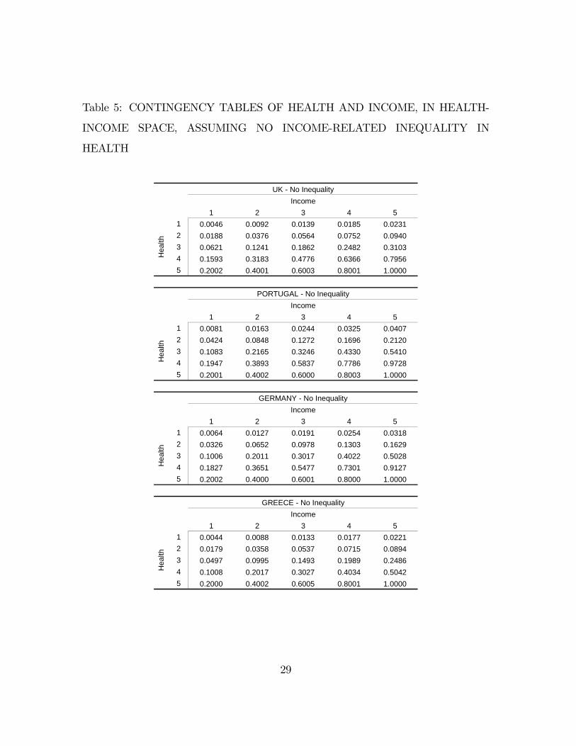
Table 5: CONTINGENCY TABLES OF HEALTH AND INCOME, IN HEALTH-

INCOME SPACE, ASSUMING NO INCOME-RELATED INEQUALITY IN

HEALTH

1 2 3 4 51 0.0046 0.0092 0.0139 0.0185 0.02312 0.0188 0.0376 0.0564 0.0752 0.09403 0.0621 0.1241 0.1862 0.2482 0.31034 0.1593 0.3183 0.4776 0.6366 0.79565 0.2002 0.4001 0.6003 0.8001 1.0000

1 2 3 4 51 0.0081 0.0163 0.0244 0.0325 0.04072 0.0424 0.0848 0.1272 0.1696 0.21203 0.1083 0.2165 0.3246 0.4330 0.54104 0.1947 0.3893 0.5837 0.7786 0.97285 0.2001 0.4002 0.6000 0.8003 1.0000

1 2 3 4 51 0.0064 0.0127 0.0191 0.0254 0.03182 0.0326 0.0652 0.0978 0.1303 0.16293 0.1006 0.2011 0.3017 0.4022 0.50284 0.1827 0.3651 0.5477 0.7301 0.91275 0.2002 0.4000 0.6001 0.8000 1.0000

1 2 3 4 51 0.0044 0.0088 0.0133 0.0177 0.02212 0.0179 0.0358 0.0537 0.0715 0.08943 0.0497 0.0995 0.1493 0.1989 0.24864 0.1008 0.2017 0.3027 0.4034 0.50425 0.2000 0.4002 0.6005 0.8001 1.0000

Hea

lth

GREECE - No InequalityIncome

Hea

lth

Income

Hea

lth

GERMANY - No InequalityIncome

UK - No InequalityIncome

Hea

lth

PORTUGAL - No Inequality

29

4 Discussion

Following Contoyannis and Wildman (2006), the contingency tables are able to show

relative cell frequencies at each intersection of SAH and income quintile. Doing so

enables further analysis or comparison of countries, in more detail than either Con-

centration Indices or copula ranking allows. Table 4.6 is used to highlight which

country is nearest to, or farthest from, the relative cell frequency that would match

independence between SAH and income. Table 4.6 shows that Germany has almost

uniformly less departure from its perfect-equality distribution, corresponding to no

association between health and income: this is not surprising, given how low its mea-

sures of association were, relative to the other countries used.

Portugal and Greece, however, now make for a more interesting comparison. Both

exhibit more income-related inequality than the UK, but not absolutely more than

one another - as evidenced by their switching with relatively minor changes in the car-

dinal scale of SAH in Table 4.2. Specifically, Portugal has a higher proportion (than

predicted for perfect equality) of people along the dimension of Very Poor health, as

well as along the highest income quintile. It also had the closest-to-expected pro-

portion of people with Very Good health, although the differences are far smaller.

Greece, on the other hand, exhibits more income-related inequalities elsewhere in

the health-income space of the contingency table. It is rank-ordered above Portugal,

though, because Portugal’s greater polarity at the lowest health and highest incomes

generates stronger rank correlation than Greece’s more wide-spread, but weaker, de-

partures from perfect equality.

5 Conclusion

This paper has demonstrated the utilisation of copulas as measures of association

between health and income, a means by which socioeconomic inequalities in health

30

Table 6: MIN AND MAX DISTANCE FROM ZERO ASSOCIATION BETWEEN

HEALTH AND INCOME IN THE BIVARIATE CDF DUE TO THE GUMBEL

COPULA

1 2 3 4 5 1 2 3 4 51 0 0 0 0 0 1 0 0 0 0 12 0 0 0 0 0 2 0 0 0 0 03 0 0 0 0 0 3 0 0 0 0 04 0 0 0 0 0 4 0 0 0 0 05 0 0 0 0 0 5 0 0 0 0 0

1 2 3 4 5 1 2 3 4 51 1 1 1 1 1 1 0 0 0 0 02 0 0 0 1 1 2 0 0 0 0 03 0 0 0 0 1 3 0 0 0 0 04 0 0 0 0 1 4 0 0 0 0 05 0 0 0 0 0 5 1 1 0 1 1

1 2 3 4 5 1 2 3 4 51 0 0 0 0 0 1 1 1 1 1 02 0 0 0 0 0 2 1 1 1 1 13 0 0 0 0 0 3 1 1 1 1 14 0 0 0 0 0 4 1 1 1 1 15 1 0 0 0 0 5 0 0 1 0 0

1 2 3 4 5 1 2 3 4 51 0 0 0 0 0 1 0 0 0 0 02 1 1 1 0 0 2 0 0 0 0 03 1 1 1 1 0 3 0 0 0 0 04 1 1 1 1 0 4 0 0 0 0 05 0 1 1 1 1 5 0 0 0 0 0

Hea

lthH

ealth

Hea

lthH

ealth

UK - Max distance

PORTUGAL - Max distance

GERMANY - Max distance

GREECE - Max distance

Hea

lth

Income

Hea

lth

Income

Hea

lth

Income

Income

Hea

lth

GERMANY - Min distance Income

GREECE - Min distance Income

UK - Min distance Income

PORTUGAL - Min distance Income

31

can be compared. The concentration curve and concentration index are considered the

standard approach to measuring and comparing inequalities in health, controlling for

individual rank in the income distribution. However, because Self-Assessed Health

is commonly measured on an ordinal scale, the concentration curve and Index are

dependent upon the cardinal scale subsequently given to health. Here I showed,

using 4 countries from the European Community Household Panel, that changing the

cardinal scale of health can re-order countries in an international comparison.

The copula method is based upon measures of rank correlation. When estimated

in a manner that accommodates the discrete scale of health, the copula measure of

association between health and income can be used comparatively as a measure of

income-related inequality in health. The copula proved to be invariant to changes in

the cardinal scales given to health. Moreover, contingency tables were shown, illus-

trating the copula in bivariate health-income space. Using this approach, departures

from perfect equality can be traced across the 2-dimensional plane of heatlh-income

space, identifying, for example, one country’s inequality being greater along the in-

come dimension, while another country’s might be greater along the health dimension.

Portugal ranks belowGreece (i.e. has stronger association between health and income,

and therefore greater income-related inequality in health), because of polarisation at

the lower end of its health distribution. Greece exhibits more widely-spread, but

smaller levels, of association elsewhere in the joint distribution of health and income.

Acknowledgements

The advice of Murray Smith, Andrew Jones, Nigel Rice and Larry Taylor con-

tributed greatly to this paper, and work done by Cristina Hernández Quevedo sim-

plified my analysis greatly. I also thank Health, Econometrics and Data Group at

the University of York. Financial support by the Centre for Health Economics is

acknowledged gratefully.

32

Notes

1That is to say, this analysis does not explicitly make any determinations of ’best’

or ’worst’ from any welfarist perspectives, only statistical perspectives.

2For income y, with rank function (or other CDF) F (y), the Lorenz curve is given

by F1 (y), where F1 is the income (or the proportion of all income) earned by all

individuals with income less than or equal to y.

3Generalised concentration curves are those that multiply a concentration curve

by total health: rather than the cumulative share of health, one sees the cumulative

amount of health. Although the horizontal axis will be the cumulative proportion of

a ranked population, the vertical axis will be the cumulative amount of health that

ranks enjoys, up to the total health in the population.

4This relates to the previous note: division of the covariance by the mean of health

is needed to force the limits of the generalised concentration index to match the Gini

coefficient - in that the cumulative share of health extends from 0 to the total health

health in the population - and facilitate more straightforward interpretation.

5For some families of copulas, closed-form solutions for either Spearman’s ρ or

Kendall’s τ may - or may not - be available. Packages such as Mathematica or

Maple, however, can be employed to find numerical solutions.

6In their study, ’not weak’ was when |τ b| > 0.02. Observed dependence in this

data not considered to be sufficiently weak for the discrete SAH to be a problem.

7Kendall’s τ b is often applied to 2 × 2 tables and/or binary data. The results in

Vandenhende and Lambert (2000) suggest that, with 5 categories in SAH, τ b can be

considered an increasing function of θ.

33

8Algebraically, the Frank copula does not nest independence because of the term1θ. Nelsen (1998), however, demonstrates that lim

θ→0CFrank = uv, i.e. the Product

Copula.

9It is also referred to, in Nelsen (1999, 2006) and Hutchinson and Lai (1990) as

the Gumbel-Hougaard copula.

10This was done by Cristina Hernández Quevedo, a colleague at the University of

York, for other research - for which I am very grateful.

11Although the question and the number of categories is different in different coun-

tries. For this analysis the countries are comparable in this regard.

12Details of the procedure, as well as Matlab and Stata codes, are available from

the author, as well as online here www.york.ac.uk/res/herd/hedg_stata.html.

13Results from the other copulas are available from the author.

14This is comparable to a bivariate cut-point.

34

REFERENCESAli, M. M., Mikhail, N. N., Haq, M. S. 1978. A class of bivariate distributions

including the bivariate logistic, Journal of Multivariate Analysis. 8: 405-412.

Allison, R. A., Foster, J. E. 2004. Measuring health inequality using qualitative

data, Journal of Health Economics. 23: 505-524.

Bommier, A., Stecklov, G. 2002. Defining health inequality: why Rawls succeeds

where social welfare theory fails, Journal of Health Economics. 21: 497-513.

Bosmans, K., Lauwers, L., Ooghe, E. 2006. A consistent multidimensional Pigou-

Dalton transfer principle. Center for Economic Studies Discussion Paper. Katholieke

Universiteit, Leuven.

Bouyé, E., Durrleman, V., Nikeghbali, A., Riboulet, G., Roncalli, T. 2000. Cop-

ulas for finance: a reading guide and some applications. Groupe de Recherche Oper-

ationnelle, Credit Lyonnais.

Braveman, P., 2006. Health disparities and health equity: concepts and measure-

ment. Annual Review of Public Health. 27: 167-94.

Cameron, A. C., Li, T., Trivedi, P. K., Zimmer, D. M., 2004. Modelling the

differences in counted outcomes using bivariate copula models with an application to

mismeasured counts. Econometrics Journal, 72: 566-584.

Chateauneuf, A., Moyes, P. 2005. Lorenz non-consistent welfare and inequality

measurement, Journal of Economic Inequality. 2(2): 1-87.

Contoyannis, P., Wildman, J. 2006. Using relative distributions to investigate

socioeconomic inequalities in the Body-Mass Index in England and Canada. Paper

presented at the 5th IHEA World Congress. Barcelona, Spain.

Dardanoni, V., Lambert, P. J. 2001. Horizontal inequity comparisons, Social

Choice. and Welfare. 18: 799-816.

35

De Castro, S., Goncalves, F., 2002. False contagion and false convergence clubs

in stochastic growth theory, Discussion Paper 237, Departamento de Economia, Uni-

versidade de Brasilia, Brasilia.

Fermanian, J-D., 2005. Goodness of fit tests for copulas, Journal of Multivariate

Analysis, 951: 119—152.

Frank, M.J., 1979. On the simultaneous associativity of F(x,y). and x + y —

F(x,y). Aequationes Mathematica, 19: 194—226.

Fredericks, G. A., Neslen, R. B., 20007. On the relationship between Spearman’s

rho and Kendall’s tau for pairs of continuous random variables, Journal of Statistical

Planning and Inference. 137: 2143-2150.

Genest, C., Rivest, L-P. 1993. Statistical inference procedures for bivariate Archim

edean copulas, Journal of the American Statistical Association. 88 (423): 1034-1043.

Hernández Quevedo, C., Jones, A. M., López Nicolás, Á., Rice, N. 2006. Socioeco-

nomic inequalities in health: a comparative longitudinal analysis using the European

Community Household Panel. Social Science and Medicine. 635: 1246-61.

International Society for Equity in Health. Working definitions 2001.

Joe, H., 1997. Multivariate Models and Dependence Concepts. Chapman and

Hall, London.

Jones, A. M., Rice, N. 2004. Using longitudinal data to investigate socio-economic

inequality in health. In: Health Policy and Economics: Opportunities and Challenges.

Smith PC, Ginnelly L, Sculpher M. eds.. Open University Press, Berkshire.

Kakwani, N., 1977. Measurement of tax progressivity: an international compari-

son. The Economics Journal. 87: 71-80.

Kakwani, N., 1980. Income Inequality and Poverty, World Bank, New York.

Kakwani, N., Wagstaff, A., van Doorslaer, E., 1997. Socioeconomic inequalities in

36

health: measurement, computation, and statistical inference, Journal of Economet-

rics. 771: 87-103.

Kolesárová, A., Mordelová, J., 2006. Quasi-copulas and copulas on a discrete

scale. Soft Computing. 106:495-501.

Leclerc, A., Lert, F., Fabien, C., 1990. Differential mortality: some comparisons

between England and Wales, Finland and France, based on inequality measures, In-

ternational Journal of Epidemiology, 19: 1001-1010.

Nelsen, R. B. 2006. An Introduction To Copulas. 2nd Ed. Springer Verlag, New

York.

Peracchi., F. 2002. The European Community Household Panel: a review. Em-

pirical Economics. 27: 63-90.

Perkins, P., Lane, T., 2003. Monte-Carlo simulation in MATLAB using copulas.

MATLAB News & Notes, November 2003.

Preston, S. H., Haines, M. R., Pamuk, E., 1981. Effects of industrialization and

urbanization on mortality in developed countries, in Solicited Papers Vol 2, HJSSP

19th International Population Conference, Manila. IUSSP, Liege, 1981.

Rosa Dias, P., Jones, A. M. 2007. Giving equality of opportunity a fair innings.

Health Economics. 16: 109-112.

Sen, A., 1973. On Economic Inequality. Norton, New York.

Sklar, A., 1959. Fonctions de répartition à n dimensions et leur marges. Publica-

tions of the Institute of Statistics. University of Paris. 8: 229-231.

Trivedi, P. K., Zimmer, D. M., 2006. Copula modeling: an introduction for

practitioners, Foundations and Trends in Econometrics, 11: 1-110.

van Doorslaer, E., Jones A. M. 2003. Inequalities in self-reported health: valida-

tion of a new approach to measurement Journal of Health Economics. 221: 61-87.

37

van Doorslaer, E., Koolman, X., 2004. Explaining the differences in income-related

health inequalities across European countries, Health Economics, 137: 609-628.

van Doorslaer, E., Wagstaff, A., Bleichrodt, H., Calonge, S., Gerdtham, Ulf-G.,

Gerfin, M., Geurts, J., Gross, L., Häkkinen, U., Leu, R. E., O’Donnell, O., Propper,

C., Puffer, F., Rodriguez, M., Sundberg, G., Winkelhake, O., 1997. Socioeconomic

inequalities in health: some international comparisons, Journal of Health Economics,

161: 93-112.

Vandenhende, F., Lambert, P., 2000. Modeling repeated ordered categorical data

using copulas, Discussion Paper 00-25, Institut de Statistique, Université catholique

de Louvain, Louvain-la-Neuve.

Vandenhende, F., Lambert, P. 2003. Improved rank-based dependence measures

for categorical data. Statistics & Probability Letters. 63: 157-163.

Wagstaff, A., van Doorslaer, E., 2000. Income inequality and health: what does

the literature tell us? Annual Review of Public Health, 21: 543-67.

Wagstaff, A., van Doorslaer, E., Paci, P. 1989. Equity in the finance and delivery

of health care: some tentative cross-country comparisons. Oxford Review of Economic

Policy. 51: 89-112.

Wagstaff, A., van Doorslaer, E., Watanabe, N. 2003. On decomposing the causes

of health sector inequalities with an application to malnutrition inequalities in Viet-

nam, Journal of Econometrics. 112: 207-223.

Wagstaff, A., Paci, P., van Doorslaer, E. 1991. On the measurement of inequalities

in health. Social Science and Medicine. 335: 545-557.

Zheng, B., 2006. Measuring health inequality and health opportunity. paper

presented at the UNU-WIDER conference. United Nations University. Helsinki.

38