Embed Size (px)
Citation preview

Using False Rings to Reconstruct LocalDrought Severity Patterns on a Semiarid River
Item Type text; Electronic Dissertation
Authors Morino, Kiyomi
Publisher The University of Arizona.
Rights Copyright © is held by the author. Digital access to this materialis made possible by the University Libraries, University of Arizona.Further transmission, reproduction or presentation (such aspublic display or performance) of protected items is prohibitedexcept with permission of the author.
Download date 01/07/2018 04:54:24
Link to Item http://hdl.handle.net/10150/194123
USING FALSE RINGS TO RECONSTRUCT LOCAL DROUGHT SEVERITY PATTERNS ON A SEMIARID RIVER
by
Kiyomi Ann Morino
_____________________
A Dissertation Submitted to the Faculty of the
DEPARTMENT OF GEOGRAPHY AND REGIONAL DEVELOPMENT
In Partial Fulfillment of the Requirements For the Degree of
DOCTOR OF PHILOSOPHY WITH A MAJOR IN GEOGRAPHY
In the Graduate College
THE UNIVERSITY OF ARIZONA
2008
2
THE UNIVERSITY OF ARIZONA
GRADUATE COLLEGE
As members of the Dissertation Committee, we certify that we have read the dissertation prepared by Kiyomi A. Morino entitled Using False Rings to Reconstruct Local Drought Severity Patterns on a Semiarid River and recommend that it be accepted as fulfilling the dissertation requirement for the Degree of Doctor of Philosophy _______________________________________________________________________ Date: April 11, 2008
Stephen R. Yool _______________________________________________________________________ Date: April 11, 2008
Katherine K. Hirschboeck _______________________________________________________________________ Date: April 11, 2008
Edward P. Glenn _______________________________________________________________________ Date: April 11, 2008
David M. Meko Final approval and acceptance of this dissertation is contingent upon the candidate’s submission of the final copies of the dissertation to the Graduate College. I hereby certify that I have read this dissertation prepared under my direction and recommend that it be accepted as fulfilling the dissertation requirement. ________________________________________________ Date: April 11, 2008 Dissertation Director: Steven R. Yool

3
STATEMENT BY AUTHOR This dissertation has been submitted in partial fulfillment of requirements for an advanced degree at the University of Arizona and is deposited in the University Library to be made available to borrowers under rules of the Library. Brief quotations from this dissertation are allowable without special permission, provided that accurate acknowledgment of source is made. Requests for permission for extended quotation from or reproduction of this manuscript in whole or in part may be granted by the head of the major department or the Dean of the Graduate College when in his or her judgment the proposed use of the material is in the interests of scholarship. In all other instances, however, permission must be obtained from the author. SIGNED: Kiyomi Ann Morino

4
ACKNOWLEDGEMENTS There are several people who have significantly contributed to the completion of this dissertation. I would first like to thank Dave Meko. Dave has been an awesome mentor to me during my graduate career. He is creative, thorough and clear-thinking, making him an outstanding researcher and communicator. As a grad student, however, I have greatly benefited from his generosity, both with his time and insights. I would also like to thank Ed Glenn for being a reluctant iconoclast. Ed’s ideas and perspectives were always thought-provoking and challenged me to refine my own ideas and perspectives. I would like to acknowledge all who provided the muscle and brain power to get this research off the ground and help move it towards its completion. I could not have completed my field work without all those who braved the foul-smelling discharge of a cored cottonwood: Margaret Adcock, Erica Bigio, Mike Burton, Rebecca Franklin, Jim McAdams, Emily Morino, Devin Petry, Dan Potts, Shawna Chartrand, and Roz Wu. Other field support was provided by Chris Baisan and Ellis Margolis. There are also number of people who tolerated, inspired and critiqued my ideas about cottonwoods and tree rings: Margaret Adcock, Toby Ault, Dave Breshears, Don Falk, Troy Knight, Ali Macalady, Amy McCoy, Pamela Nagler, Rachel Pfister, Dan Potts, Russ Scott, Scott St. George, Julie Stromberg, and many others. And although they were not directly involved with this research, I want to acknowledge my interactions with Tom Swetnam and Chris Baisan early on in my graduate career. I am quite certain their passion for tree rings and field work played a huge role in starting me off on this journey. Funding for this research came from a variety of sources, including a grant from the USGS, the Technology and Research Initiative Fund (TRIF), and multiple teaching assistantships provided by the Department of Geography and Regional Development and the Laboratory of Tree-Ring Research. I deeply appreciate the support of my family. Thanks to my Mom and Jim who were always eager to don their hiking boots and come down with me to the San Pedro. Thanks to my Mom, who taught me how to work hard and who has been an unflagging source of encouragement throughout my life. Thanks to my Dad, who always stressed the importance of following your heart and who gave me the courage to take risks. And thanks to my brother, who has always been very excited about my work even though he wasn’t always quite sure what it was about. And last but not least, I am forever indebted to Margaret without whom this work would simply not have been possible.

5
DEDICATION
This dissertation is dedicated to my parents, Emily and Dick
for their love and encouragement.

6
TABLE OF CONTENTS LIST OF TABLES ............................................................................................................................9 LIST OF FIGURES........................................................................................................................10 ABSTRACT.......................................................................................................................................12 CHAPTER 1: INTRODUCTION .............................................................................................14 1.1 Statement of Problem...................................................................................................14 1.2 Background.....................................................................................................................15
1.2.1 Drought.........................................................................................................................15 1.2.2 Water sources for riparian trees.................................................................................16 1.2.3 Surface and ground water connections ....................................................................17 1.2.4 Seasonal drought..........................................................................................................18 1.2.5 Tree-ring response to seasonal drought ...................................................................18 1.2.6 Why tree rings?.............................................................................................................19
1.3 Organization of dissertation...........................................................................................20 CHAPTER 2: PRESENT STUDY ............................................................................................22 2.1 Documenting riparian false rings under field conditions .................................22 2.2 Documenting riparian false rings under controlled conditions ......................22 2.3 False-ring chronologies on the San Pedro River..................................................23 2.4 Major Conclusions ........................................................................................................24
2.4.1 False rings as indicators of zero-flow conditions....................................................24 2.4.2 Riparian tree growth response to artificial drought................................................25 2.4.3 Increasing drought severity on the San Pedro River ..............................................25
WORKS CITED ..............................................................................................................................27 APPENDIX A – TREE GROWTH RESPONSE TO ZERO-FLOW EVENTS: CAN TREE RINGS BE USED TO RECONSTRUCT STREAMFLOW INTERMITTENCY? ....................................................................................................................30 A.1 Abstract .......................................................................................................................................31 A2. Introduction...............................................................................................................................31 A.3 Methods and Materials...........................................................................................................35
A.3.1 Site Description...............................................................................................................35 A.3.2 Data Collection ...............................................................................................................37 A.3.3. Data Analysis..................................................................................................................38
A.4 Results .........................................................................................................................................39 A.4.1 Tree-ring Data .................................................................................................................39
A.4.1.1. Radial Growth Patterns .....................................................................................39 A.4.1.2 Identifying False Rings........................................................................................40
A.4.2 Hydrological Data..........................................................................................................40 A.4.2.1 Stage and Groundwater data..............................................................................40 A.4.2.2 Diurnal Groundwater Fluctuations...................................................................42
7
A.5 Discussion..................................................................................................................................43 A.6 Summary and Conclusions....................................................................................................48 A.7 Acknowledgements .................................................................................................................50 A.8 Works Cited ...............................................................................................................................51 A.9 Figure Captions ........................................................................................................................66 APPENDIX B: FALSE-RING RESPONSE IN COTTONWOOD AND WILLOW TO ARTIFICIAL DROUGHT ...................................................................................................68 B.1 Abstract .......................................................................................................................................69 B.2 Introduction...............................................................................................................................69 B.3 Methods and Materials...........................................................................................................71
B.3.1 Plant Materials .................................................................................................................71 B.3.2 Soil Moisture....................................................................................................................72 B.3.3 Sapflow .............................................................................................................................72 B.3.4 Stress Treatments............................................................................................................73 B.3.5 Tree core samples and wood analysis ..........................................................................74 B.3.6 Analysis.............................................................................................................................75
B.4 Results.........................................................................................................................................76 B.4.1 Soil Moisture Profiles .....................................................................................................76 B.4.2 Sapflow .............................................................................................................................77 B.4.3 Annual Growth and False Rings in 2006 ....................................................................78 B.4.4 Digital Analysis of False Rings......................................................................................80
B.5 Discussion..................................................................................................................................80 B.5.1 Differences between willow and cottonwood ............................................................81 B.5.2 Recovery following short-term drought ......................................................................83 B.5.3 Quantifying false rings....................................................................................................83 B.5.4 Application to Field Conditions ...................................................................................84
B.6 Summary and Conclusions ...................................................................................................85 B.7 Acknowledgements .................................................................................................................86 B.8 Works Cited ...............................................................................................................................87 B.9 Figure Captions ......................................................................................................................101 APPENDIX C: FALSE RINGS IN COTTONWOOD (POPULUS FREMONTII): TREE-RING EVIDENCE FOR AN INTENSIFICATION OF DROUGHT IN A SEMIARID RIVER ECOSYSTEM ........................................................................................ 104 C1. Abstract .....................................................................................................................................105 C.2 Introduction.............................................................................................................................105 C.3 Methods and Materials .......................................................................................................109
C.3.1 Study Area..................................................................................................................... 109 C.3.2 Climate........................................................................................................................... 109 C.3.3 Hydrology ..................................................................................................................... 110 C.3.4 Study Sites ..................................................................................................................... 111 C.3.4 Sampling and Sample Preparation............................................................................. 112 C.3.5 Data Analysis ................................................................................................................ 112
C.3.5.1 Response Variable............................................................................................. 113

8
C.3.5.2 Potential Explanatory Variables ..................................................................... 113 C.3.5.3 Logistic Regression Analysis ........................................................................... 115
C.4 Results.......................................................................................................................................116 C.4.1 False-ring Chronologies .............................................................................................. 116 C.4.2 Logistic Regression Models........................................................................................ 117
C.4.2.1 False-ring Chronologies and Explanatory Variables ................................... 117 C.4.2.2 Final Models ...................................................................................................... 118
C.5 Discussion................................................................................................................................119 C.6 Summary and Conclusions .................................................................................................126 C.7 Acknowledgements .............................................................................................................. 127 C.8 Works Cited .............................................................................................................................128 C.9 Figure Captions ......................................................................................................................144

9
LIST OF TABLES Table A1 A chronology of events related to false-ring formation in cottonwood characterized by depth to groundwater (DGW)............................................................................57 Table A2. Studies with data indicating the effect of ~1 m decreases in groundwater levels on survivorship of mature cottonwood trees. .....................................................................................58 Table C1: Pearson correlation coefficients for pair-wise comparisons amongst explanatory variables. .......................................................................................................................................... 133 Table C2. Logistic regression models for BCG, CHM and FRB. ........................................ 134
10
LIST OF FIGURES
Figure A1 Area and site maps. .......................................................................................................59 Figure A2. Hydroclimatology of the study area. ........................................................................60 Figure A3. Hypothesized configuration of the monitoring well, tree with dendrometer, and channel at our site. ...........................................................................................................................61 Figure 4. Relative growth of four instrumented cottonwood throughout the growing season. ...............................................................................................................................................................62 Figure A5. Cottonwood false-ring morphology. .........................................................................63 Figure A6. Hydrological data for 2002. ........................................................................................64 Figure A7. Amplitude of diurnal fluctuations. .............................................................................65 Figure B1. Configuration of cottonwood-willow experimental grove. .....................................93 Figure B2. Identifying false rings with image analysis. ...............................................................94 Figure B3. Soil moisture profiles for each of the three treatments over the course of the experiment...........................................................................................................................................95 Figure B4. Minimum average soil moisture recorded at each depth for each treatment.........96 Figure B5. Sap velocity for each species by treatment..................................................................97 Figure B6. Boxplots of brightness indices for one core/tree in each treatment. .....................98 Figure B7. Soil moisture profiles of trees C4 and D4 compared to average soil moisture profiles for the High Stress Group and the Control Group. ....................................................99 Figure B8. Average daily sap velocity for Control Group outliers, C4 (circles) and D4 (triangles).. ........................................................................................................................................ 100 Figure C1. Study area and site locations. ................................................................................... 135 Figure C2. Hydroclimatology of the study area. ......................................................................... 136 Figure C3. Raw false-ring chronologies for each site: BCG, CHM, and FRB. ...................... 137 Figure C4. Adjusted false-ring chronologies for each site: BCG, CHM, and FRB. .............. 138

11
LIST OF FIGURES - Continued Figure C5. Pearson correlation coefficients between the response variable (logit(P), where P is the proportion of false rings) and each of the potential explanatory variables. ................. 139 Figure C6. Logistic regression models for FRB.......................................................................... 140 Figure C7. Logistic regression results for CHM......................................................................... 141 Figure C8. Temporal patterns of ANN, MASS, and DRY over the period of record. ...... 142 Figure C9. Number of low-flow days during May, June and July over the period of record............................................................................................................................................................. 143

12
ABSTRACT In this research, I describe the use of false rings to reconstruct local histories of seasonal
drought in riparian ecosystems in semiarid regions. In tree-ring analysis, false rings are
boundary-like features often formed as a response to drought within the growing season.
Drought can be a common feature in hydrologic regimes of dryland rivers but in recent
decades drought has been intensifying due to climate change and increasing water use by
cities, agriculture and industry. Identifying when and where water availability has decreased
along the river course is critical for understanding, and therefore managing, these generally
endangered ecosystems. The higher density of trees compared to instrumental data make
them ideal candidates for reconstructing site-specific drought patterns.
The first part of this dissertation is an observational study conducted on the San Pedro River
in southeastern Arizona during 2002. I used dendrometer data and local hydrological data to
show that a period of negligible radial growth in cottonwood during the middle of the
growing season coincided with a channel drying event. Tree-ring core samples confirmed
that false-rings had formed in each of the instrumented trees. The second part of this
dissertation is an experimental study designed to evaluate the effect of different levels of
water stress on false-ring formation in cottonwood and willow. I showed that experimental
decreases in water availability for periods as short as ten days were enough to induce false-
ring formation in willow. Longer periods of reduced water availability were generally
required to induce false-ring formation in cottonwood. In the final part of this dissertation,
I reconstructed false-ring occurrence in Fremont cottonwoods at three sites along the San
Pedro River. I infer from false-ring frequencies that the severity of summer drought has

13
been increasing over the last four to six decades but that the drought severity varies along a
hydrological gradient. Overall, the findings in this body of research confirm that false rings
in riparian tree species can be used as indicators of seasonal drought and underscore the
importance of identifying site-specific responses to reduced water availability along the
riparian corridor.

14
CHAPTER 1: INTRODUCTION
1.1 Statement of Problem
The San Pedro River in southeastern Arizona is a unique place. Its headwaters are located in
northern Mexico, just south of the United States-Mexico border. From there, it flows
northward into Arizona, winding through the desert landscape until it eventually meets and
joins with the Gila River. In 1988, Congress designated an approximately 65 km stretch,
beginning roughly at the international border, as a Riparian National Conservation Area, the
first of its kind in the United States. Congress was rightly impressed by the disproportionate
contribution of such a small area to regional biodiversity. The impetus to conserve and
maintain the San Pedro Riparian National Conservation Area can also be justified in several
other arenas. As a riparian landscape, the San Pedro River corridor provides essential
ecosystem services, including water filtering and flood control. Additionally, healthy riparian
ecosystems in semiarid regions can have tremendous economic value in terms of eco-
tourism, recreation and property values (Bark-Hodgins and Colby 2006, Weber and Berrens
2006).
In June of 2005, the longest recording streamflow gage on the San Pedro River registered,
for the first time in its 100-year history, a flow of zero. Since then, the gage has gone dry
multiple times, always during the late spring and early summer, a dry and warm period just
prior to the onset of the summer rains. Low- and zero-flow events are defining
characteristics of streamflow regimes in dryland rivers. Nevertheless, because of the
historical perspective afforded by the gage record, the zero-flows at the Charleston gage

15
were and are cause for concern amongst resource managers. Decreases in water availability
can lead to decreases in biodiversity (Stromberg and others 2007).
The observed drying trend is not unique to the San Pedro River. A greater proportion of
limited water supplies are being appropriated on a global scale by growing human
populations, ultimately leaving less water for riparian ecosystems. Moreover, in some areas,
reduced rainfall and higher temperatures have further exacerbated dry conditions. The
spatial character of shifts to drier conditions along the river course is however difficult to
characterize. Streamflow gages provide an excellent local record but are often too few to
adequately characterize spatial variability in dryland streamflow regimes. Indeed, the San
Pedro River has been dubbed an “interrupted perennial stream,” meaning that reaches with
intermittent streamflow occur discontinuously over the length of the river course (Leenhouts
and others 2006). Data indicate that the Charleston reach is drying up, but how is drought
being manifested on other stretches of the river?
To address this question, I employ tree-ring analysis. As a somewhat novel approach, I use
false rings (intra-annual ring boundaries) to reconstruct local drought chronologies at three
sites along the San Pedro River. To gain a better understanding of false-ring formation, I
also examine hydrological conditions that are favorable to false-ring formation, both in field
and greenhouse settings.
1.2 Background
1.2.1 Drought
16
Although the term drought is widely used, it is not easily defined. Rasmussen and others
(1993) provide a widely applicable definition of drought, stating that it is generally associated
with “a sustained period of significantly lower soil moisture levels and water supply relative
to the normal levels around which the local environment and society have stabilized.” This
definition identifies an essential quality of an effective drought definition: that decreases in
water availability are evaluated within the context of a specific system. Additionally, this
definition highlights some of the challenges in defining drought: definitions must identify,
first, what constitutes significantly lower levels of water availability, and second, what
constitutes a stable system.
In the following, I will begin by discussing how drought affects overstory trees in semiarid
riparian ecosystems. I will conclude by introducing the use of false rings for providing a
temporal context to evaluate drought severity in semiarid riparian ecosystems.
1.2.2 Water sources for riparian trees
Overstory trees are a key structural component of riparian landscapes. The composition and
distribution of riparian forests within the floodplain plays an important role in governing
ecosystem function. The primary cause of drought for overstory trees is a low water table
but soil moisture levels can also influence drought status in some cases. In a study to
identify water sources used by riparian trees, Snyder and Williams (2000) found that Fremont
cottonwood (Populus fremontii.) uses soil moisture to supplement its groundwater supply when
it is available but Goodding’s willow (Salix gooddingii) appears to use only groundwater, even
when soil moisture is available. Despite the flexibility demonstrated by species such as
17
Fremont cottonwood, trees of any species become entirely dependent on groundwater
during periods of no or negligible rainfall.
1.2.3 Surface and ground water connections
Water table fluctuations in floodplain aquifers are inextricably linked with streamflow. For
this reason, streamflow can be a reliable indicator of depth to groundwater for streamside
trees (Rood and others 2003). The movement of water between the channel and floodplain
aquifer is governed by subsurface hydrological gradients. When water tables occur at a
higher elevation than river stage (the elevation of the surface of the water in the channel),
water is discharged from the aquifer into the channel; reaches where this occurs are called,
“gaining” reaches. Conversely, when river stage is higher than water table elevations, water
is discharged from the channel into the aquifer; reaches where this occurs are called “losing”
reaches.
The spatial distribution of gaining and losing reaches depends on the configuration and
composition of the floodplain aquifer. Losing reaches occur in segments of the floodplain
that generally store larger amounts of water than the volume of recharge they receive. These
segments will be relatively wide and deep, and/or comprised mostly of coarse alluvia with
high water-holding capacities. The converse is true for gaining reaches. During a multi-year
drought, water table elevations in the floodplain aquifer will begin to decrease basin-wide
and a larger proportion of the river course will consist of losing reaches (Dahm and others
2003).

18
1.2.4 Seasonal drought
Trees growing along losing reaches are more likely to be exposed to drought on a seasonal
basis. Seasonal fluctuations of groundwater levels tend to occur over a larger range of
groundwater depths along losing reaches (Lite and Stromberg 2005). Initial responses of
trees to drought include certain biochemical adjustments (Larcher 2003) but within weeks
expansive growth (irreversible cell enlargement) will be reduced (Bradford and Hsiao 1982).
When seasonal drought is followed by a moisture pulse that enables expansive growth to
resume, the drought event may be permanently recorded in the tree’s anatomy as a false ring.
1.2.5 Tree-ring response to seasonal drought
False rings have been observed and derived experimentally by withholding water in both
conifers and angiosperms. In conifers, they are identified by tracheids of reduced radial
diameter (Larson 1963, Glerum 1970, Barnett 1976). Initial visual assessments of false rings
led researchers to describe false rings as having thick-walled, latewood-type cells (Kuo and
McGinnies 1973). Actual measurements reveal that cell-wall thickness in false rings is in fact
the same as earlywood cells (Vaganov and others 2006). In angiosperms, the greater
complexity of ring anatomy precludes a general description of false rings. For example, in
teak (Tectonis grandis), Priya and Bhat (1998) identified four types of false rings based on
unique combinations of fiber, parenchyma and vessel cell characteristics.
For both conifers and angiosperms, false rings are generally less distinctive than true rings.
They may exhibit more gradual cell transitions and/or be less bright. During more extreme
droughts, false rings can be morphologically indistinguishable from true rings. When false
rings are essentially identical to true rings, they are identified by employing a

19
dendrochronological technique known as crossdating, the comparison of relative patterns of
ring width amongst different trees. Indeed, the initial scientific investigations of false rings
were conducted by dendrochronologists (Schulman 1939, Glock and Reed 1940). The
potential for using false rings as environmental indicators was first recognized almost 60
years ago by Glock (1951) but it wasn’t until 1980 that false rings were used in a climate-
ecology study (Wimmer and others 2002). False rings continue to be an under-utilized
source of environmental information (Wimmer and others 2000, Masiokas and Villalba
2004).
1.2.6 Why tree rings?
Like all tree-ring studies, the strength of false-ring analysis is that it provides an unrivalled
temporal perspective. Even false-ring chronologies only a few decades long can contribute
important information about the dynamics of seasonal drought on semiarid rivers. The
spatial heterogeneity of streamflow in dryland rivers is often such that wet and dry reaches
may alternate several times between adjacent streamflow gages (Walker and others 1995,
Smakhtin 2001, Stromberg and others 2006). A local record, no matter how short, offers
infinitely more information than no record at all.
Given an extended record, it becomes possible to identify shifts, trends and anomalous
years. Drought is a common occurrence in semiarid regions and constitutes an important
driver of riparian ecosystem form and function (Poff and Ward 1989, Lake 2003, McMahon
and Finlayson 2003, Lite and Stromberg 2005, Stromberg and others 2007). Increasing
frequency and intensity of drought can nevertheless be detrimental, as organisms are less

20
likely to be equipped to deal with intensified drought. Armed with information regarding
the location and extent of intensifying drought, resource managers can then proceed with
developing management strategies to avoid, or at least mitigate, potentially undesirable
outcomes.
1.3 Organization of dissertation
This dissertation consists of a submitted and accepted manuscript that appears as Appendix
A and two pre-publication manuscripts that appear as Appendices B and C.
The first manuscript (Appendix A) is entitled, “Tree growth response to zero-flow events:
Can tree rings be used to reconstruct streamflow intermittency?” It was submitted and
accepted with revision to the journal of Environmental Management. For this part of my
research, I collected, prepared and analyzed all dendrometer and tree-ring data; I analyzed
groundwater data that was collected by one of my co-authors, Russ Scott of the United
States Department of Agriculture; and I wrote the manuscript. My co-authors on this
manuscript are Russ Scott, David Meko and Ed Glenn.
The second manuscript (Appendix B) is entitled, “False-ring response in cottonwood and
willow to artificial drought.” For this part of my research, I designed the experiment,
collected and analyzed soil moisture, sapflow and tree-ring data and wrote the manuscript.
My co-author on this manuscript is Ed Glenn.

21
The final manuscript (Appendix C) is entitled “False rings in cottonwood (Populus fremontii):
Tree-ring evidence for an intensification of drought in a semiarid river system.” For this
part of my research, I collected, prepared and analyzed tree-ring data and wrote the
manuscript. My co-authors on this manuscript are David Meko and Katie Hirschboeck.
22
CHAPTER 2: PRESENT STUDY
The following text summarizes the approach and major findings for each of the three studies
that comprise my dissertation research. The studies, with details and complete descriptions,
can be found in the appendices.
2.1 Documenting riparian false rings under field conditions
In this study, I used manual dendrometers to track radial growth in cottonwood growing
along an intermittent reach on the San Pedro River in southeastern Arizona. I collected
radial growth data during the growing season of 2002. One of the primary objectives of this
study was to evaluate the potential for reconstructing zero-flow events using false rings. I
compared dendrometer data to local hydrological data. High-resolution groundwater data
was provided by Russ Scott of the United States Department of Agriculture; high-resolution
stage data was provided by James Leenhouts of the United States Geological Survey. I
analyzed dendrometer data and hydrological data and found that mid-season growth in
cottonwood abruptly stopped for a period of time that roughly coincided with the period of
time when the channel was dry. Zero growth in cottonwood occurred for the period of time
when groundwater depths were greater than 2.5 meters. I used groundwater data to infer
that this was the depth where roots lost contact with the water table. I concluded that,
under certain conditions, false rings can be reliable indicators of zero-flow events.
2.2 Documenting riparian false rings under controlled conditions
In this study, I designed a drought experiment to elucidate factors influencing false-ring
formation in two prominent riparian tree genera, cottonwood (Populus spp.) and willow (Salix
23
spp.). I exposed three species of trees: P. deltoides, P. fremontii, and S. gooddingii, to two levels of
drought in an outdoor grove consisting of 4-5 year-old saplings planted in a grid pattern.
The low-stress treatment was defined by a 66% reduction in water availability over a period
of 10 days; the high-stress treatment was defined by a 66% reduction in water availability
over a 19 day period. I measured sapflow and collected soil moisture data over the course of
the experiment. Sapflow rates responded very quickly to both reductions and increases in
water availability. False rings were formed in all three species with willow tending to show a
higher propensity for false-ring formation. Willow was more likely to form false rings in the
low-stress treatment and in the high-stress treatment, willow false rings tended to be more
distinctive (brighter) than cottonwood false rings.
2.3 False-ring chronologies on the San Pedro River
In this study, I cored streamside cottonwood (P. fremontii) at three different sites along the
San Pedro River in southeastern Arizona. Sites were located along a hydrological gradient
based on streamflow presence throughout the year. I prepared and crossdated samples in
the lab and compiled false-ring chronologies for each site. Chronologies consisted of the
proportion of trees exhibiting a false ring in a given year. In each site, false-ring occurrence
was marked by a quasi-periodic pattern superimposed upon an increasing trend. I used
logistic regression to model how temperature and a subset of hydrological variables
influenced rates of false-ring formation. I was unable to fit a model at the wettest site but
the best available models at the intermediate and dry sites suggested some intriguing patterns
in the hydrological drivers of false-ring formation. At the intermediate site, a relatively
wetter site, false-ring formation appeared to be driven more by variability in drought length;

24
whereas, at the dry site, false-ring formation appeared to be driven more by variability in
recharge.
2.4 Major Conclusions
2.4.1 False rings as indicators of zero-flow conditions
The formation of a false ring not only depends on presence of drought but also the
opportunity for recovery. False rings where formed following an approximately three week
period when root access to groundwater had been significantly reduced. Drought was
terminated by the onset of the summer rains. Recovery may have been compromised by a
longer drought and/or by less precipitation during the summer rainy season.
Field observations of false-ring formation in cottonwood compared with onsite hydrological
data suggest that false rings may in some cases be a reliable indicator of zero-flow
conditions. Given that growth in riparian trees responds primarily to fluctuations in shallow
groundwater, the use of false rings to reconstruct zero-flow events assumes that surface and
ground waters have a strong hydrological connection. Next, the relationship between false-
ring formation and zero-flow conditions hinges upon the relative elevations of maximum
root depth and the thalweg (lowest point of the channel). When these two elevations are
similar, false-ring formation will more likely represent zero-flow conditions. In the cases
when false rings do not signify zero-flow conditions, they are still a valuable source of
information regarding patterns of water availability for riparian trees and how these patterns
may be changing over space and time.
25
2.4.2 Riparian tree growth response to artificial drought
Results of controlled experiments are not directly applicable to field conditions due to the
simplified conditions of controlled experiments. Nevertheless, by creating an artificial
drought, I demonstrated that: 1) reduced water availability is a key factor in false-ring
formation and 2) there appear to be differences in false-ring expression between species for
a similar level of drought stress. Riparian trees exhibit high sensitivity to reductions in water
availability. Decreases in sapflow were observed within 3-4 days of decreases in water
availability. Sustained low water levels and subsequent replenishment of water supplies
resulted in the formation of false rings. This study marks the first time that false rings have
been artificially induced in riparian tree species. Moreover, false-ring intensity, as indicated
by brightness profiles, appears to differ both among species and between treatments.
Willow was most susceptible to false-ring formation. Compared to cottonwood, more
willows formed false rings in the low-stress treatment (decreased water availability for 10
days) and willow false rings in the high-stress treatment (decreased water availability for 19
days) tended to be brighter than cottonwood. The difference in false-ring expression
between cottonwood and willow may be due to willow’s greater drought sensitivity, faster
growth rate, or a combination of both.
2.4.3 Increasing drought severity on the San Pedro River
The use of false rings can be a rich source of information for understanding hydrological
drought at a local level within semiarid riparian landscapes. False-ring chronologies
developed from streamside cottonwood (P. fremontii) along the San Pedro River in
southeastern Arizona reveal that mid-summer drought severity has been gradually increasing
26
over the last 40 to 60 years. Superimposed upon this gradual increase is a quasi-periodic
pattern where peak occurrences of drought occur roughly at seven- to ten-year intervals.
Possible sources of hydrological drought are decreases in annual streamflow and increases in
duration of summer low flow, depending on relative amount of available water. For drier
sites, low levels of recharge appear to play an important role in false-ring formation; for
wetter sites, duration of summer low flow shows a strong relationship with false-ring
formation. Possible drivers of hydrological drought include near stream groundwater
pumping and increases in vegetation cover.
The magnitude of drought severity appeared to vary according to position along the
hydrological gradient: wet, intermediate and dry. The site with the greatest increase in false-
ring occurrence is the intermediate site which is currently intermittent but appears to have
had non-limiting levels of water availability in the near past. Lower increases in false-ring
occurrence were observed in trees located at the dry site. False-ring data from the dry site
suggest that these trees have been exposed to significant summer drought throughout most
of their lives. The contrast in false-ring occurrence between the intermediate and dry sites is
consistent with Shafroth and others (2000) who found that riparian trees establishing under a
groundwater regime characterized by a relatively stable water table will tend to be less
adapted to groundwater-induced drought conditions than those establishing under a
groundwater regime where the water table fluctuated over relatively large ranges in depth
over the course of the growing season.
27
WORKS CITED
Bark-Hodgins R, Colby BG (2006) An economic assessment of the Sonoran Desert Conservation Plan. Natural Resources Journal 46:709-725
Barnett JR (1976) Rings of collapsed cells in Pinus radiata stemwood from lysimeter-grown
trees subjected to drought. New Zealand Journal of Forestry Science 6:461-465 Bradford KJ, Hsiao TC (1982) Physiological responses to moderate water stress. In: Lang
OL, Noble PS, Osmond CB, Ziegler H (eds) Encyclopedia of Plant Physiology. Springer-Verlag, Vienna, Austria, p 264-324
Dahm CN, Baker MA, Moore DI, Thibault JR (2003) Coupled biogeochemical and
hydrological responses of streams and rivers to drought. Freshwater Biology 48:1219-1231
Glerum C (1970) Drought ring formation in conifers. Forest Science 16:246-248 Glock WS (1951) Cambial Frost Injuries and Multiple Growth Layers at Lubbock, Texas.
Ecology 32:28-36 Glock WS, Reed EL (1940) Multiple growth layers in the annual increments of certain trees
at Lubbock, Texas. Science 91:98-99 Kuo M, McGinnies EA (1973) Variation of anatomical structure of false rings in eastern
redcedar. Wood Science 5:205-210 Lake PS (2003) Ecological effects of perturbation by drought in flowing waters. Freshwater
Biology 48:1161-1172 Larcher W (2003) Physiological Plant Ecology: Ecophysiology and Stress Physiology of
Functional Groups Vol. Springer, New York
28
Larson PR (1963) The indirect effect of drought on tracheid diameter in red pine. Forest Science 9:52-62
Leenhouts JM, Stromberg J, Scott RL (2006) Hydrologic requirements of and consumptive
use by riparian vegetation along the San Pedro River, Arizona. U.S. Geological Survey Scientific Investigations Report 2005-5163
Lite SJ, Stromberg JC (2005) Surface water and ground-water thresholds for maintaining
Populus-Salix forests, San Pedro River, Arizona. Biological Conservation 125:153-167 Masiokas M, Villalba R (2004) Climatic significance of intra-annual bands in the wood of
Nothofagus pumilio in southern Patagonia. Trees-Structure and Function 18:696-704 McMahon TA, Finlayson BL (2003) Droughts and anti-droughts: the low flow hydrology of
Australian rivers. Freshwater Biology 48:1147-1160 Poff NL, Ward JV (1989) Implications of streamflow variability and predictability for lotic
community structure - A regional analysis of streamflow patterns. Canadian Journal of Fisheries and Aquatic Sciences 46:1805-1818
Priya PB, Bhat KM (1998) False ring formation in teak (Tectona grandis Lf) and the influence
of environmental factors. Forest Ecology and Management 108:215-222 Rasmussen EM, Dickinson RE, Kutzbach JE, Cleaveland MK (1993) Climatology. In:
Maidment DR (ed) Handbook of Hydrology. McGraw-Hill, New York Rood SB, Braatne JH, Hughes FMR (2003) Ecophysiology of riparian cottonwoods: stream
flow dependency, water relations and restoration. Tree Physiology 23:1113-1124 Schulman E (1939) Classification of false annual rings in west Texas pines. Tree-Ring
Bulletin 6:3 Shafroth PB, Stromberg JC, Patten DT (2000) Woody riparian vegetation response to
different alluvial water table regimes. Western North American Naturalist 60:66-76

29
Smakhtin VU (2001) Low flow hydrology: a review. Journal of Hydrology 240:147-186 Snyder KA, Williams DG (2000) Water sources used by riparian trees varies among stream
types on the San Pedro River, Arizona. Agricultural and Forest Meteorology 105:227-240
Stromberg JC, Beauchamp VB, Dixon MD, Lite SJ, Paradzick C (2007) Importance of low-
flow and high-flow characteristics to restoration of riparian vegetation along rivers in and south-western United States. Freshwater Biology 52:651-679
Stromberg JC, Lite SJ, Rychener TJ, Levick LR, Dixon MD, Watts JM (2006) Status of the
riparian ecosystem in the upper San Pedro River, Arizona: Application of an assessment model. Environmental Monitoring and Assessment 115:145-173
Vaganov EA, Hughes MK, SHashkin AV (2006) Growth Dynamics of Conifer Tree Rings
Springer-Verlag, Berlin Walker KF, Sheldon F, Puckridge JT (1995) A Perspective on Dryland River Ecosystems.
Regulated Rivers-Research & Management 11:85-104 Weber MA, Berrens RP (2006) Value of instream recreation in the Sonoran Desert. Journal
of Water Resources Planning and Management-Asce 132:53-60 Wimmer R, Downes GM, Evans R (2002) High-resolution analysis of radial growth and
wood density in Eucalyptus nitens, grown under different irrigation regimes. Annals of Forest Science 59:519-524
Wimmer R, Strumia G, Holawe F (2000) Use of false rings in Austrian pine to reconstruct
early growing season precipitation. Canadian Journal of Forest Research-Revue Canadienne De Recherche Forestiere 30:1691-1697

30
APPENDIX A – TREE GROWTH RESPONSE TO ZERO-FLOW EVENTS: CAN TREE RINGS BE USED TO RECONSTRUCT STREAMFLOW
INTERMITTENCY?
Kiyomi A. Morino, Russell L. Scott, Edward P. Glenn, and David M. Meko.
31
A.1 Abstract
Characterizing local streamflow regimes has become an integral part of developing
conservation strategies for riparian landscapes. In semiarid regions, absence of flow
constitutes a critical driver of ecosystem structure and function. Yet, the low density of
streamflow gages combined with the generally high spatial variability of zero-flow conditions
along river courses make it difficult to describe even basic parameters of zero-flow regimes,
such as frequency of occurrence. In this study, we explored the use of tree rings as
indicators of zero-flow events. We hypothesized that a temporary loss of surface flow
during the growing season would result in the formation of a false ring—an intra-annual ring
boundary—in riparian trees. On the San Pedro River in southeastern Arizona, we tracked
radial growth rates in cottonwood, Populus fremontii, and local hydrology over the course of a
growing season using a manual dendrometer. We found that cessation in radial growth
coincided with a period of zero flow. Disappearance of diurnal fluctuations in groundwater
data suggests that roots became stranded above the water table at a depth of about 2.5 m,
after a groundwater decline of approximately 0.5 m. Vertical hydrological connectivity was
restored after a period of about three weeks, coinciding with return of streamflow at the
study site. Core samples revealed false rings were morphologically distinct from true rings.
We hypothesize that leaf shedding may play a significant role in the formation of false rings
for this species. Caveats and optimal conditions for interpreting cottonwood false rings as
indicators of zero-flow events are discussed.
A2. Introduction
32
Characterizing streamflow regimes is an integral component to developing restoration and
conservation plans for threatened and endangered river systems throughout the United
States (Stromberg and Patten 1990, Poff and others 1997, Richter and others 1997). Our
ability, however, to accurately represent streamflow variability over time and space is largely
restricted by data availability. In addition to the limited length of many streamflow records,
characterizing streamflow regime is further constrained limited spatial coverage. Streamflow
gages constitute point data and are often sparsely distributed along the river’s length (Poff
and others 2006). These shortcomings are exacerbated for rivers and streams in arid and
semiarid regions, where stream gage density is particularly low and streamflow variability,
both temporal and spatial, is high (Walker and others 1995, Smakhtin 2001).
One uncertainty that arises from too few streamflow gages in semiarid watersheds is the
characterization of zero-flow events. While the identification of potentially intermittent
reaches can be estimated based on geomorphological characteristics (Stanley and others
1997), the temporal patterns of no-flow conditions for a given reach are largely unknown
(Stromberg and others 2007). Absence of surface water constitutes a critical regulatory
process in dryland environments and is considered an integral, and perhaps defining,
characteristic of streamflow regimes in dryland environments (Poff and Ward 1989, Lake
2003, McMahon and Finlayson 2003, Lite and Stromberg 2005, Stromberg and others 2007).
Channel drying tends to exhibit high spatial variability along semiarid river courses, thus dry
conditions can prevail in relatively close proximity to gages recording flowing water. For
example, on the Upper San Pedro River Basin in southeastern Arizona, gage records during

33
the dry season show continuous flow while not far downstream, field data reveal stretches of
river channel alternating between wet and dry (Stromberg and others 2006).
At sub-gage spatial scales, one potential source of information on streamflow intermittency
is tree rings. The hydrological connection between surface water and shallow groundwater
makes streamflow a reasonable proxy for water available to floodplain trees. Riparian tree
rings have been analyzed for a variety of hydrological applications, including: ascertaining the
impact of streamflow regulation and dam construction (Reily and Johnson 1982, Dudek and
others 1998); determining instream flow requirements (Stromberg and Patten 1990, 1996);
and evaluating drought stress (Leffler and Evans 1999, Potts and Williams 2004). In one of
the few studies conducted on a reach with intermittent streamflow, Clark (1987) reported no
relationship between streamflow and radial growth. In comparison, Stromberg and Patten
(1996) reported a significant, positive relationship between tree growth and streamflow on
sites with intermittent flow. The range of growth rates reported during zero-flow years was
however too wide to identify zero-flow years based on ring widths alone.
The apparent absence of a relationship between tree-ring width and streamflow
intermittency does not preclude using tree-rings to reconstruct zero-flow events.
Intermittent streams tend to flow on a seasonal basis; although during very dry periods, flow
can be absent the entire year (Gordon and others 2004). When zero-flow conditions occur
within the growing season, tree growth may be interrupted, manifesting in the formation of a
false ring. These intra-annual growth bands are ring boundary-type features formed within
the growing season as a response to stress (Fritts 1976). False rings have long been
34
recognized in forestry (Jones 1931) and were carefully described by early
dendrochronologists to ensure accurate dating of wood specimens (Schulman 1939, Glock
and Reed 1940) but have only recently been used as environmental indicators (Wimmer and
others 2000, Masiokas and Villalba 2004). False rings can be formed as a result of air
pollution (Kurczynska and others 1997), insect defoliation (Priya and Bhat 1998, Salleo and
others 2003, Heinrich and Banks 2006), floods (Young and others 1993) and low
temperatures (Kozlov and Kisternaya 2004).
False rings have previously been observed in cottonwood (Stromberg 1998, Leffler and
Evans 1999), but the environmental conditions leading to their formation have not yet been
described. Our main interest is the role of drought, or low water availability, in the
formation of false rings in cottonwood. False rings formed as a result of drought have been
found to be associated with a period of dry conditions within the growing season for both
conifers and broad-leaved trees, (Villalba and Veblen 1996, Wimmer and others 2000,
Cherubini and others 2003, Masiokas and Villalba 2004). Similarly, false rings have been
induced experimentally in both conifers and broad-leaved trees by withholding water
(Larson 1963, Glerum 1970, Barnett 1976, Priya and Bhat 1998).
We have selected the San Pedro River basin, in southeastern Arizona, to conduct our study
as it provides an ideal setting to evaluate the association between streamflow intermittency
and false-ring formation in riparian trees. Early summer is marked by little or no
precipitation and is combined with high temperatures. During this period, streamflow is at a
minimum (Pool and Coes 1999). In early July, the summer rainy season starts, resulting in a

35
pulse of moisture that recharges depleted hydrological reserves. Our primary goal in this
study was to relate growth of streamside trees to fluctuations in water availability. We
characterized radial growth patterns of cottonwood (Populus fremontii) and compared these
with fluctuations in groundwater elevations and river stage over the course of a year. We
hypothesized that a zero-flow event, when accompanied by physiologically-significant
declines in the alluvial water table, would lead to the formation of a false ring.
A.3 Methods and Materials
A.3.1 Site Description
The study site was located on the San Pedro River in southeastern Arizona (Figure A1). The
San Pedro River is a low-gradient alluvial river that flows northward from its headwaters in
Mexico to its confluence with the Gila River in Arizona, USA. Our study area was located
within the San Pedro Riparian National Conservation Area (SPRNCA). Established in 1988,
the SPRNCA covers a 50 km stretch of the river that has an intact and high-quality riparian
ecosystem. The largest urban areas in the basin and adjacent to the SPRNCA are the city of
Sierra Vista and the military post of Fort Huachuca. The US portion of the upper basin (i.e.,
the Sierra Vista sub-watershed) is home to approximately 66,000 people. Groundwater is a
primary source of water for the human population in the basin and it is also essential for the
maintenance of the perennial flow and riparian ecosystem within the SPRNCA. Some
groundwater modeling studies show that groundwater pumping has already reduced water
availability in the San Pedro River floodplain (Pool and Dickinson 2007).
36
The climate in the upper basin along the river is semiarid with a mean annual total
precipitation of around 350 mm and a mean annual average temperature of 17.5 °C (Figure
A2). Precipitation is typically concentrated in two parts of the year. The summer season,
spanning roughly July to September, is driven by convective storms that generate around
60% of annual total precipitation. The winter season, spanning roughly December through
March, is driven by Pacific frontal systems and accounts for much of the remaining portion
of the annual total. Perhaps the most predictable part of the annual cycle is the dry fore-
summer or pre-monsoon season from around April to July. May and June are particularly
dry, averaging 5.3 and 12.7 mm, respectively. June is also one of the hottest months of the
year averaging 25.7 °C.
The closest streamflow monitoring station to the site is the USGS Charleston gage, located
approximately 4.5 km upstream of the study site. Baseflow, the majority of which is
discharge of groundwater from the regional aquifer, has tended to ensure perennial flow at
the gage during the late spring and early summer (Pool and Coes 1999). Baseflow, however,
constitutes a small proportion of annual streamflow. The majority of streamflow is derived
from storm runoff, which is much greater and more variable in summer than in winter (Pool
and Coes 1999). Storm runoff also plays an important role in recharging the alluvial aquifer
and significantly buffers baseflow (Baillie and others 2007). Streamflow tends to be lowest
during May and June when riparian evapotranspiration rates are high and precipitation is low
(Figure A2).
37
Overstory vegetation on the San Pedro River is dominated by Fremont cottonwood (P.
fremontii) and Goodding’s willow (Salix gooddingii). These gallery forests are discontinuously
distributed along the banks and floodplains of the river. Our study area is located along a
losing reach of an entrenched stretch of the river (Figure A1). On the right bank, where our
study was conducted, there are approximately equal numbers of cottonwoods and willows
but the basal area of cottonwood was approximately double that of willow. Based on a total
census, average diameters of cottonwoods and willows were 31.9±22.7 cm and 22.8±15.5
cm, respectively.
A.3.2 Data Collection
On March 18, 2002 (Day of Year 77), constant-tension manual band dendrometers
(Agricultural Electronics Corporation, Tucson, AZ) were affixed to four cottonwood trees,
ranging in size from 29.2 to 87.2 cm in diameter, located along the bank within 12 m from
the thalweg. After a period of adjustment (approximately 2 weeks), to allow for the tree to
grow into the band, data collection commenced (April 3, 2002, DOY 93). At this point, tree
crowns were fully developed. Tree growth was measured as increases in circumference over
the course of the growing season. Data were collected between 9:00 and 11:00 am every 1-2
weeks. Increments of growth were measured to the nearest 0.5 mm. At the end of the
growing season, each of the four cottonwood trees was cored at a height of about 1.5 m.
Cores samples were mounted on grooved wooden strips, then surfaced using a razor blade.
Tree-ring features for 2002 were evaluated using a dissecting microscope.
38
River stage was measured in a persistent pool, and two monitoring wells were used to
characterize seasonal water table dynamics at our site (Figure A1). Stage and water table
elevations were logged every 30 minutes using a water level recorder (miniTROLL, In Situ,
Laramie, WY). Monitoring wells were located on a higher-level terrace, leading to
overestimated groundwater depths with respect to streamside trees, specifically during the
second half of the growing season (Figure A3). We therefore interpolated depth to
groundwater (DGW) between the stage and the closest well to the stage recorder, c2d, to
estimate DGW at the location of the study trees (Figure A1). Estimated DGW was most
accurate for tree CHL06, the banded tree closest to the stage-well transect.
A.3.3. Data Analysis
We plotted dendrometer data as cumulative growth, normalized by total growth of the tree
over the growing season. This enabled direct comparison of intra-seasonal growth rates
between trees despite differences in size. Growth curves were then compared to 30-minute
groundwater data to identify groundwater depth, rate of decline and presence/absence of
diurnal fluctuations for different phases of radial growth.
In addition to longer-term (weekly to monthly) patterns in seasonal DGW, we were able to
obtain a record of diurnal groundwater fluctuations throughout the growing season. Daily
cycles of transpiration induce a daily cycle of groundwater fluctuation at sites where plants
depend on groundwater to maintain internal water balance (White 1932). During the dry
season, transpiration is the primary source of discharge in floodplain environments. Daily
minima (relatively deep groundwater) occur in the later afternoon when transpiration stops;
39
daily maxima (relatively shallow groundwater) occur after dawn when transpiration begins.
In this study, we did not use diurnal groundwater fluctuations to estimate specific
transpiration rates; rather, we used these data to indicate relative differences in transpiration
rates over the course of the growing season.
We employed a two-step process to illustrate variability in diurnal signal strength over time.
First, we detrended groundwater data. A trend line was constructed using a low-pass
Gaussian filter. One advantage of using a filter versus simply smoothing the data by other
methods, for example averaging, is that filtering enables complete control over the
frequencies retained in the data. We set our filter window to retain variability generated by
cycles greater than 24 hours. These frequencies were subsequently removed by subtracting
the resultant trend line from the raw data. For the second step, we took the difference
between minima and maxima for each day in the detrended series and divided by two. The
final time series showed daily amplitudes of diurnal groundwater fluctuations. We
subsequently utilized these amplitudes as a proxy for strength of diurnal signal.
A.4 Results
A.4.1 Tree-ring Data
A.4.1.1. Radial Growth Patterns
Dendrometer data indicate that radial growth in cottonwood began in early April and ended
around the end of October. Despite their differences in size, radial growth patterns of the
four instrumented trees varied in a relatively coherent fashion throughout the growing
season. A striking feature of these data is that all trees showed a period of negligible growth
40
in the middle of the growing season (Figure A4). According to dendrometer data, the onset
of this hiatus occurs around the beginning of June (DOY157) for two trees and the end of
June for the other two trees (DOY177). This 20-day disparity may be overestimated because
we lack data between these two dates. The end of this hiatus appears to be more
synchronous with increases in relative growth occurring about a week and a half into July
(~DOY190).
A.4.1.2 Identifying False Rings
False rings were observed in core samples from for all four banded trees. False rings were
identified by: 1) a less clear ring boundary, manifesting as a duller and/or less sharp
boundary; 2) a lower number of vessel elements in contact with the boundary feature; and 3)
an apparent lower density of vessel elements following the false ring (Figure A5). The extent
to which these characteristics were expressed varied both within and between trees.
A.4.2 Hydrological Data
A.4.2.1 Stage and Groundwater data
Although stage data are incomplete, they show, in conjunction with groundwater data, some
important features of the local hydrology. First, the relative positions of water elevations for
stage and groundwater data indicate that, during our study, the stream was losing (or
influent) at this reach (Figure A6). On June 18 (DOY 169), surface flow ceased, thus
marking the onset of zero-flow conditions. Following the loss of surface flow, rates of
groundwater decline appear to increase, likely due the absence of recharge supplied by
surface water. The exact date of return of streamflow to our study site is unknown because
41
of missing stage data but it was between July 8 (DOY189), when a local rain event (data
collected onsite) dropped 6.86 mm of precipitation, and July 17 (DOY 198), when
groundwater depths began to rapidly increase. On July 9, streamflow at the Charleston gage
increased from 0.03 cms to 0.05 cms (data not shown). The next increase at the Charleston
gage is on July 15 (DOY 196) to 0.07 cms. Then on July 16 and 17, two very large rain
events are recorded locally, dropping 15.24 and 18.03 mm of precipitation, respectively.
After about mid-August, when monsoon intensity subsided and flood frequency decreased,
both stage and groundwater elevations decreased again (Figure A6). Floods in early to mid-
September (~DOY 240-260) led to a corresponding increase in groundwater elevations and
may also have prevented a second zero-flow event late in the season. Beginning about early
October (~DOY 280), both stage and groundwater elevations started to rise again.
Two gaps in the stage data created corresponding gaps in estimated groundwater depths at
tree CHL06. For the first block of missing data, we estimated depth to groundwater using a
linear interpolation between May 6 and June 3 (DOY 127-155). For the second block of
missing data (July 3 to July 16; DOY 185-198), groundwater depth at well c2d appeared to
be a reasonable indicator of groundwater depth at tree CHL06. Similar to groundwater data
at well c2d, stage data indicated accelerated decline once the thalweg elevation was breached
(Figure A6). By comparison to groundwater decline at well c2d, however, water levels in the
persistent pool decreased at a faster rate. This led to similar water table elevations recorded
at both the monitoring well and stage recorder by about June 29 (DOY 180), five days prior
to the second data gap in recorder data (Figure A6). Based on maximum groundwater depth
42
at well c2d, maximum groundwater depth at tree CHL06 was estimated to be 3.30 m but
because CHL06 is located closer to the channel than well c2d, maximum groundwater depth
at CHL06 was likely to be less than 3.30 m.
A.4.2.2 Diurnal Groundwater Fluctuations
Diurnal fluctuations were recorded throughout the year, both in the dormant and growing
season (Figure A7). We computed average fluctuation amplitudes for a 30-day period in the
dormant season (DOY 330 – 360) to establish a baseline fluctuation amplitude against which
we could compare growing season amplitudes. During this period, wells showed an average
amplitude of 1.4 and 0.9 mm for c2d and c3, respectively. Beginning around April 5 (DOY
95), diurnal amplitudes began to increase above their respective baseline levels. Between
November 5 and 9 (DOY 309 and 313), diurnal amplitudes decreased to average dormant
season levels.
A notable feature of these data for all wells is the virtual absence of diurnal groundwater
fluctuations during the middle of the growing season (Figure A7). Diurnal amplitude is so
low it falls below baseline levels during June 23 to July 17 (DOY 174 – 196) for well c2d and
June 20 to July 17 (DOY 171 to 198) for well c3. The period of attenuated diurnal
fluctuation begins after groundwater level has decreased 32 and 42 cm, falling at a rate of
1.44 and 1.58 cm day -1 for wells c2d and c3, respectively. This period of near-zero
amplitudes is preceded by a period of decreasing amplitudes beginning on June 2 and 3
(DOYs 153 and 154), in wells c3 and c2d, respectively (Figure A7), and is followed by a
43
series of large and short-lived increases in amplitude reflect flood events that raised stage
elevation by at least 0.5 m (data not shown).
A.5 Discussion
We hypothesized that zero-flow conditions, when they occur within the growing season and
are associated with water table declines, would be associated with false-ring formation in
cottonwood trees. And indeed, in 2002, we observed both zero-flow conditions and false-
ring formation in each of the sampled trees. Streamflow is however only a proxy of water
available to riparian trees. Groundwater depths are more direct indicators of water
availability, especially during seasonal drought. Moreover, high-resolution groundwater data
that track diurnal fluctuations provide a way to evaluate the effect of decreasing groundwater
on tree physiological function. Understanding the relationship between zero-flow
conditions and false-ring formation is important for evaluating if, where, and when
cottonwood false rings might be used to reconstruct streamflow intermittency.
Combining dendrometer, stage and groundwater depth data, we developed a hydrological
chronology identifying surface and sub-surface conditions potentially related to physiological
stress and false-ring formation (Table A1). We identified three stages of tree response to
fluctuating water availability based on: 1) amplitude variability in diurnal fluctuations, or
relative strength of diurnal signal, in groundwater data (HyG in Table A1); and 2)
dendrometer measurements (D in Table A1). By comparison, groundwater data was a more
precise indicator of tree response to environmental conditions owing to its higher temporal
resolution—thirty-minute intervals—compared to one to three week intervals for radial
44
growth measurements. The first stage, Level I Stress, marks initial physiological adjustments
and preceded the onset of zero-flow conditions. Level II Stress indicates the next phase of
stress and was realized during zero-flow conditions. The last stage, Recovery, appeared to
coincide with channel re-wetting.
Initial responses of trees to environmentally-induced stress were characterized by a decrease
in transpiration rate, and therefore water use, and a cessation of radial expansion. Both
responses are indicative of stomatal adjustments to water deficits (Larcher 2003). When
water availability decreases, stoma remain open for less time. Stomatal closure
simultaneously limits the amount of water lost to the environment, thus conserving plant
water balance, and decreases CO2 assimilation, thus reducing growth potential. In this study,
Level I Stress began prior to zero-flow conditions when water tables are relatively high,
suggesting trees were responding to some other environmental factor. At another reach
with intermittent streamflow on the San Pedro River, Gazal and others (2006) observed an
almost identical pattern of plant water use where transpiration rates began to decrease at the
beginning of June when groundwater levels were relatively shallow, and trees were
presumably not water limited. The authors attributed reduced transpiration rates to high
vapor-pressure deficits (the difference between saturation and atmospheric vapor pressure;
VPD). Similarly, along the Bill Williams River, in southern Arizona, decreases in stomatal
conductance occurred in the absence of drought stress during a period of high VPD
(Horton and others 2001a).
45
It does not appear that atmospheric stress alone can induce false-ring formation. Even
though high VPDs are seasonal in southern Arizona, occurring in early summer, no false
ring was observed in any of the core samples from the study trees in 2001, and stage data
indicate that during 2001 no zero-flow conditions occurred. Moreover, trees along reaches
with perennial streamflow do not exhibit the same level of stress, demonstrated by reduced
transpiration rates, as do trees along reaches with intermittent streamflow (Gazal and others
2006).
Stomatal closure in response to high VPD, as opposed to water deficit, was not widely
considered until the 1970s (Jones 1992) and has since been described as an anticipatory
response to water deficits yet to come (Bradford and Hsiao 1982). In semiarid riparian
landscapes, atmospheric stress does indeed give way to drought stress along losing reaches
where channels dry up and water tables continue to fall for as long as dry periods persist
(Dahm and others 2003). The impact of groundwater depth on riparian trees is often
reported as change in relative depth, as vertical root extent of mature trees varies according
to groundwater regimes occurring during early phases in growth (Albertson and Weaver
1945, Shafroth and others 2000). One indicator of drought stress in riparian trees is when
roots become stranded above the water table. This event appears to be manifested in
groundwater data as a loss of diurnal signal (Butler and others 2007). In our study, a
decrease of diurnal fluctuation amplitudes to negligible levels marks the onset of Stress Stage
II and occurred after a drop in groundwater depth of about 0.5 meters (Table A1). Some
studies imply that vertical hydrological disconnection can occur with declines as low at 0.3
m for coarse substrates (Cooper and others 2003). Data from Gazal and others (2006)
46
suggest that a 0.4 m decline in groundwater depth marked the onset of drought stress. In
this study, trees continued to transpire at very low levels up to a groundwater decline of 0.9
m.
When roots become stranded above the water table, depth to groundwater ceases to be
physiologically relevant. Instead, duration that roots are stranded becomes an indicator of
ability to recover. For example, intra-annual groundwater declines of 1 m lasting multiple
growing seasons have been found to result in widespread mortality amongst mature trees,
while shorter exposures to comparable changes in groundwater depth have had varying
results (Table A2). Based on limited data, it appears that mature cottonwood trees can
withstand one-meter declines in groundwater for up to about a month before some trees
begin to die. For rapid declines in groundwater depth, leaves will begin to turn yellow and
senesce after 2-3 weeks, with an average crown reduction of 34% after 3-5 days (Scott and
others 1999, Cooper and others 2003). Timing, rate and extent of senescence may vary
when groundwater decline is more gradual, as well as when drought stress is preceded by
atmospheric stress. At our site, each of the four study trees exhibited a 50-90% crown
reduction after 20 days into Stress Stage II (K.Morino, unpublished notes, 2002).
Recovery from drought is a critical stage in the process of false-ring formation and must
occur within the growing season. Cottonwood recovery has been documented in field
studies for both directly-induced (Amlin and Rood 2003, Cooper and others 2003) and
indirectly-induced (Horton and others 2001b, Gazal and others 2006) drought. Radial
growth appears to resume between July 20 and 27 (DOY 200-207); identification of an exact
47
date is precluded by the sampling interval of dendrometer data (Figure A4). Our ability to
precisely identify timing of recovery based on groundwater data is impeded by the
overwhelming signature of flood pulses in diurnal fluctuation data (Figure A7). By July 23
(DOY 203), amplitudes appear somewhat stable and register as greater than average
amplitudes during Stress Stage II. Even without a “flood-pulse” effect, groundwater data
may be conservative estimate of when recovery begins. Cottonwood, in particular those
growing along intermittent reaches, have been found to utilize soil moisture when available
(Snyder and Williams 2000). Thus, local rain events occurring on July 8, 16, and 17 (DOY
189, 197&198) may have initiated the recovery process before groundwater levels began to
increase. Further restricting the use of groundwater data to evaluate recovery is that if trees
were exploiting soil moisture, the transpiration signal in groundwater data would have been
muted (Butler et al. 2007).
Assuming that study trees represented crown conditions for our site, it is understandable
that recovery is initially slow. Dendrometer data indicate about a two-week lag before radial
growth rates compare to pre-monsoon growth rates (Figure A4). Based on diurnal
fluctuation amplitudes, it appears to take about 3-5 weeks before transpiration rates realize
post-drought maximum rates (Figure A7). By comparison, maximum diurnal amplitudes in
the second part of the growing season are less than during the first part of the growing
season. This may be related to the higher humidities, therefore lower atmospheric demand,
associated with the rainy season (Gazal and others 2006) or the availability of soil moisture,
either from rain events or overbank flooding (Butler et al 2007). Alternatively, crown
48
recovery may have been incomplete, resulting in lower leaf areas compared to pre-drought
leaf areas.
Intra-seasonal crown reduction and recovery may play an important role in forming the
morphological features that enable identification of false rings. Leaves, especially younger
leaves, are a primary source of auxin, a plant hormone which is thought to be a major
stimulus for cambial development (Aloni 2001, Dengler 2001). A reduction in leaf area may
therefore result in a corresponding reduction in cambial activity, possibly inducing the onset
of ring-boundary formation. If the cambium is reactivated before ring boundary features are
completed, the resultant boundary will appear less distinct than a true boundary. Auxin is
also particularly important for vessel production in trees with diffuse-porous ring structures
(like cottonwood; Aloni 2001). We hypothesize that a lower density of leaves at the onset of
tree recovery will result in a reduced rate of vessel production, and thereby a lower density of
vessels in the vicinity of the false ring compared to the true ring.
A.6 Summary and Conclusions
Our study suggests that the ability of false rings to represent zero-flow conditions depends
on two key factors. The first is the configuration of root depths, thalweg elevation, water
table elevations and horizontal gradients. Zero-flow conditions are more likely to be
associated with false-ring formation when a dry channel signifies or portends a water table
elevation below or at the maximum rooting depth of trees. The second is drought intensity.
False rings represent tree response to a particular intensity of drought stress. In this study,
we have defined drought intensity as being proportional to the amount of time roots are

49
stranded above the water table. Extent of crown reduction may be an important indicator
for identifying the minimum duration of vertical hydrological disconnection associated with
false-ring formation. Our study offered no insights regarding the maximum limit but
literature suggests that around two months, the potential for recovery becomes significantly
compromised (see Table A2). One caveat to consider in semiarid regions is that drought
stress can be preceded by atmospheric stress, thus prolonging the duration of stress period
for the plants.
Our study provides intriguing evidence that channel drying may be related to false-ring
formation. Despite limited temporal and spatial scope, our data are consistent with other
studies documenting the general environmental conditions—mid-season growth reduction
due to drought—that have resulted in false-ring formation in other species. This association,
if widely applicable, could be an asset in the characterization of streamflow regimes in arid
and semiarid regions. In any case, false-rings in riparian trees at least provide a spatial-
temporal characterization of changes in local hydrological conditions. The importance of
zero-flow events as a major force influencing riparian ecosystem structure and function and
the current lack of instrumentation to adequately characterize the temporal and spatial
variability of these events, underscores the potential of riparian false rings to significantly
contribute to our understanding of ecosystem dynamics and ecosystem response to changes
in the hydrological regime.

50
A.7 Acknowledgements: This work was supported by the United States Geological Survey
Groundwater Resources Program (Agreement No. 99WRAG0043). Michael Burton, Ellis
Margolis and Christopher Baisan provided valuable field assistance.
51
A.8 Works Cited
Albertson FW, Weaver JE (1945) Injury and death or recovery of trees in prairie climate.
Ecological Monographs 15:393-433 Aloni R (2001) Foliar and axial aspects of vascular differentiation: Hypotheses and evidence.
Journal of Plant Growth Regulation 20:22-34 Amlin NM, Rood SB (2003) Drought stress and recovery of riparian cottonwoods due to
water table alteration along Willow Creek, Alberta. Trees-Structure and Function 17:351-358
Baillie MN, Hogan JF, Ekwurzel B, Wahi AK, Eastoe CJ (2007) Quantifying water sources
to a semiarid riparian ecosystem, San Pedro River, Arizona. Journal of Geophysical Research-Biogeosciences 112:S02
Barnett JR (1976) Rings of collapsed cells in Pinus radiata stemwood from lysimeter-grown
trees subjected to drought. New Zealand Journal of Forestry Science 6:461-465 Bradford KJ, Hsiao TC (1982) Physiological responses to moderate water stress. In: Lang
OL, Noble PS, Osmond CB, Ziegler H (eds) Encyclopedia of Plant Physiology. Springer-Verlag, Vienna, Austria, p 264-324
Butler JJ, Kluitenberg GJ, Whittemore DO, Loheide SP, Jin W, Billinger MA, Zhan XY
(2007) A field investigation of phreatophyte-induced fluctuations in the water table. Water Resources Research 43
Cherubini P, Gartner BL, Tognetti R, Braker OU, Schoch W, Innes JL (2003) Identification,
measurement and interpretation of tree rings in woody species from mediterranean climates. Biological Reviews 78:119-148
Clark S (1987) Potential use of cottonwoods in dendrogeomorphology and paleohydrology.
MS Thesis, University of Arizona
52
Cooper DJ, D'Amico DR, Scott ML (2003) Physiological and morphological response patterns of Populus deltoides to alluvial groundwater pumping. Environmental Management 31:215-226
Dahm CN, Baker MA, Moore DI, Thibault JR (2003) Coupled biogeochemical and
hydrological responses of streams and rivers to drought. Freshwater Biology 48:1219-1231
Dengler NG (2001) Regulation of vascular development. Journal of Plant Growth
Regulation 20:1-13 Dudek DM, McClenahen JR, Mitsch WJ (1998) Tree growth responses of Populus deltoides
and Juglans nigra to streamflow and climate in a bottomland hardwood forest in central Ohio. American Midland Naturalist 140:233-244
Fritts H (1976) Tree Rings and Climate, Academic Press, London, UK Gazal RM, Scott RL, Goodrich DC, Williams DG (2006) Controls on transpiration in a
semiarid riparian cottonwood forest. Agricultural and Forest Meteorology 137:56-67 Glerum C (1970) Drought ring formation in conifers. Forest Science 16:246-248 Glock WS, Reed EL (1940) Multiple growth layers in the annual increments of certain trees
at Lubbock, Texas. Science 91:98-99 Gordon ND, McMahon TA, Finlayson BL, Gippel CJ, Nathan RJ (2004) Stream Hydrology:
An Introduction for Ecologists, John Wiley & Sons, Ltd., New York Heinrich I, Banks JCG (2006) Variation in phenology, growth, and wood anatomy of Toona
sinensis and Toona ciliata in relation to different environmental conditions. International Journal of Plant Sciences 167:831-841
Horton JL, Kolb TE, Hart SC (2001a) Physiological response to groundwater depth varies
among species and with river flow regulation. Ecological Applications 11:1046-1059
53
Horton JL, Kolb TE, Hart SC (2001b) Responses of riparian trees to interannual variation in ground water depth in a semi-arid river basin. Plant Cell and Environment 24:293-304
Jones HG (1992) Plants and Microclimate: A Quantitative Approach to Environmental Plant
Physiology, Cambridge University Press, New York Jones JM (1931) Prediction of seasonal precipitation in California. Monthly Weather
Review:2 Kozlov V, Kisternaya M (2004) Architectural wooden monuments as a source of
information for past environmental changes in Northern Russia. Palaeogeography Palaeoclimatology Palaeoecology 209:103-111
Kurczynska EU, Dmuchowski W, Wloch W, Bytnerowicz A (1997) The influence of air
pollutants on needles and stems of Scots pine (Pinus sylvestris L.) trees. Environmental Pollution 98:325-334
Lake PS (2003) Ecological effects of perturbation by drought in flowing waters. Freshwater
Biology 48:1161-1172 Larcher W (2003) Physiological Plant Ecology: Ecophysiology and Stress Physiology of
Functional Groups Springer, New York Larson PR (1963) The indirect effect of drought on tracheid diameter in red pine. Forest
Science 9:52-62 Leffler AJ, Evans AS (1999) Variation in carbon isotope composition among years in the
riparian tree Populus fremontii. Oecologia 119:311-319 Lite SJ, Stromberg JC (2005) Surface water and ground-water thresholds for maintaining
Populus-Salix forests, San Pedro River, Arizona. Biological Conservation 125:153-167 Masiokas M, Villalba R (2004) Climatic significance of intra-annual bands in the wood of
Nothofagus pumilio in southern Patagonia. Trees-Structure and Function 18:696-704
54
McMahon TA, Finlayson BL (2003) Droughts and anti-droughts: the low flow hydrology of Australian rivers. Freshwater Biology 48:1147-1160
Poff NL, Allan JD, Bain MB, Karr JR, Prestegaard KL, Richter BD, Sparks RE, Stromberg
JC (1997) The natural flow regime. Bioscience 47:769-784 Poff NL, Olden JD, Pepin DM, Bledsoe BP (2006) Placing global stream flow variability in
geographic and geomorphic contexts. River Research and Applications 22:149-166 Poff NL, Ward JV (1989) Implications of streamflow variability and predictability for lotic
community structure - A regional analysis of streamflow patterns. Canadian Journal of Fisheries and Aquatic Sciences 46:1805-1818
Pool DR, Coes AL (1999) Hydrogeologic Investigations of the Sierra Vista Subwatershed of
the Upper San Pedro Basin, Cochise County, Southeast Arizona. USGS Water-Resources Investigations Report 99-4197:41
Pool DR, Dickinson JE (2007) Ground-water flow model of the Sierra Vista Subwatershed
and Sonoran portions of the Upper San Pedro Basin, southeastern Arizona, United States, and northern Sonora, Mexico. U.S. Geological Survey Scientific Investigations Report 2006-5228
Potts DL, Williams DG (2004) Response of tree ring holocellulose delta C-13 to moisture
availability in Populus fremontii at perennial and intermittent stream reaches. Western North American Naturalist 64:27-37
Priya PB, Bhat KM (1998) False ring formation in teak (Tectona grandis Lf) and the influence
of environmental factors. Forest Ecology and Management 108:215-222 Reily PW, Johnson WC (1982) The effects of altered hydrologic regime on tree growth along
the Missouri River in North-Dakota. Canadian Journal of Botany-Revue Canadienne De Botanique 60:2410-2423
Richter BD, Baumgartner JV, Wigington R, Braun DP (1997) How much water does a river
need? Freshwater Biology 37:231-249
55
Salleo S, Nardini A, Raimondo F, Lo Gullo MA, Pace F, Giacomich P (2003) Effects of defoliation caused by the leaf miner Cameraria ohridella on wood production and efficiency in Aesculus hippocastanum growing in north-eastern Italy. Trees-Structure and Function 17:367-375
Schulman E (1939) Classification of false annual rings in west Texas pines. Tree-Ring
Bulletin 6:3 Scott ML, Shafroth PB, Auble GT (1999) Responses of riparian cottonwoods to alluvial
water table declines. Environmental Management 23:347-358 Shafroth PB, Stromberg JC, Patten DT (2000) Woody riparian vegetation response to
different alluvial water table regimes. Western North American Naturalist 60:66-76 Smakhtin VU (2001) Low flow hydrology: a review. Journal of Hydrology 240:147-186 Snyder KA, Williams DG (2000) Water sources used by riparian trees varies among stream
types on the San Pedro River, Arizona. Agricultural and Forest Meteorology 105:227-240
Stanley EH, Fisher SG, Grimm NB (1997) Ecosystem expansion and contraction in streams.
Bioscience 47:427-435 Stromberg J (1998) Dynamics of Fremont cottonwood (Populus fremontii) and saltcedar
(Tamarix chinensis) populations along the San Pedro River, Arizona. Journal of Arid Environments 40:133-155
Stromberg JC, Beauchamp VB, Dixon MD, Lite SJ, Paradzick C (2007) Importance of low-
flow and high-flow characteristics to restoration of riparian vegetation along rivers in and south-western United States. Freshwater Biology 52:651-679
Stromberg JC, Lite SJ, Rychener TJ, Levick LR, Dixon MD, Watts JM (2006) Status of the
riparian ecosystem in the upper San Pedro River, Arizona: Application of an assessment model. Environmental Monitoring and Assessment 115:145-173
56
Stromberg JC, Patten DT (1990) Riparian vegetation instream flow requirements - a case-study from a diverted stream in the eastern Sierra-Nevada, California, USA. Environmental Management 14:185-194
Stromberg JC, Patten DT (1996) Instream flow and cottonwood growth in the eastern Sierra
Nevada of California, USA. Regulated Rivers-Research & Management 12:1-12 Villalba R, Veblen TT (1996) A tree-ring record of dry spring-wet summer events in the
forest-steppe ecotone, northern Patagonia, Argentina In: Dean JS, Meko DM, Swetnam TW (eds) Tree Rings, Environment, and Humanity. Radiocarbon, Tucson, AZ, p 107-116
Walker KF, Sheldon F, Puckridge JT (1995) A perspective on dryland river ecosystems.
Regulated Rivers-Research & Management 11:85-104 White WN (1932) A method of estimating groundwater supplies based on discharge by
plants and evaporation from soil. In: USGS (ed). US Government Printing Office Wimmer R, Strumia G, Holawe F (2000) Use of false rings in Austrian pine to reconstruct
early growing season precipitation. Canadian Journal of Forest Research-Revue Canadienne De Recherche Forestiere 30:1691-1697
Young PJ, Megonigal JP, Sharitz RR, Day FP (1993) False ring formation in Baldcypress
(Taxodium-Distichum) saplings under 2 flooding regimes. Wetlands 13:293-298
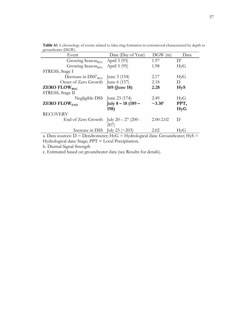
57
Table A1 A chronology of events related to false-ring formation in cottonwood characterized by depth to groundwater (DGW).
Event Date (Day of Year) DGW (m) Data Growing SeasonBEG April 3 (93) 1.97 Da
Growing SeasonBEG April 5 (95) 1.98 HyG STRESS, Stage I
Decrease in DSSbBEG June 3 (154) 2.17 HyG
Onset of Zero Growth June 6 (157) 2.18 D ZERO FLOWBEG 169 (June 18) 2.28 HyS STRESS, Stage II
Negligible DSS June 23 (174) 2.49 HyG ZERO FLOWEND July 8 – 18 (189 –
198) ~3.30c PPT,
HyG RECOVERY
End of Zero Growth July 20 – 27 (200 -207)
2.00-2.02 D
Increase in DSS July 23 (~203) 2.02 HyG a. Data sources: D = Dendrometer; HyG = Hydrological data: Groundwater; HyS = Hydrological data: Stage; PPT = Local Precipitation. b. Diurnal Signal Strength c. Estimated based on groundwater data (see Results for details).
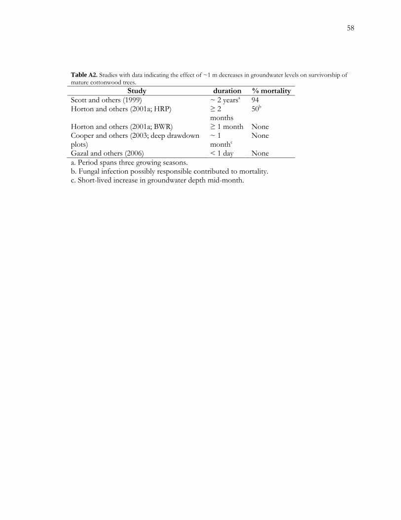
58
Table A2. Studies with data indicating the effect of ~1 m decreases in groundwater levels on survivorship of mature cottonwood trees.
Study duration % mortality Scott and others (1999) ~ 2 yearsa 94 Horton and others (2001a; HRP) ≥ 2
months 50b
Horton and others (2001a; BWR) ≥ 1 month None Cooper and others (2003; deep drawdown plots)
~ 1 monthc
None
Gazal and others (2006) < 1 day None a. Period spans three growing seasons. b. Fungal infection possibly responsible contributed to mortality. c. Short-lived increase in groundwater depth mid-month.
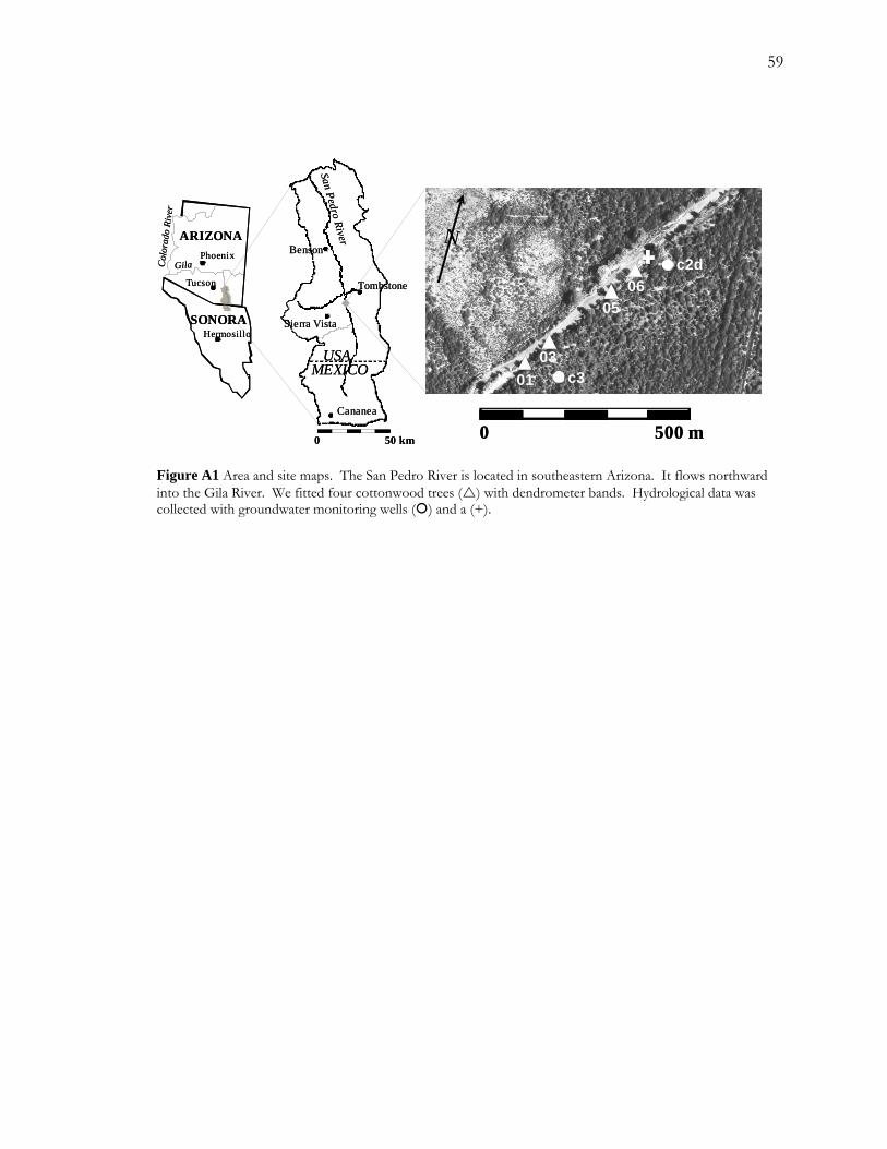
59
Phoenix
ARIZONA
SONORA
Tucson
Gila
Hermosillo
Col
orad
oRi
ver
Phoenix
ARIZONA
SONORA
Tucson
Gila
Hermosillo
Col
orad
oRi
ver
0 50 km
SanPedro
River
USAMEXICO
Cananea
Benson
Tombstone
Sierra Vista
0 50 km
SanPedro
River
USAMEXICO
Cananea
Benson
Tombstone
Sierra Vista
0 500 m0 500 m
Approximateextent of
mesquite woodland
N
Forest
Approximateextent of
mesquite woodland
N
0103
0506
c2d
c3
Figure A1 Area and site maps. The San Pedro River is located in southeastern Arizona. It flows northward into the Gila River. We fitted four cottonwood trees ( ) with dendrometer bands. Hydrological data was collected with groundwater monitoring wells ( ) and a (+).
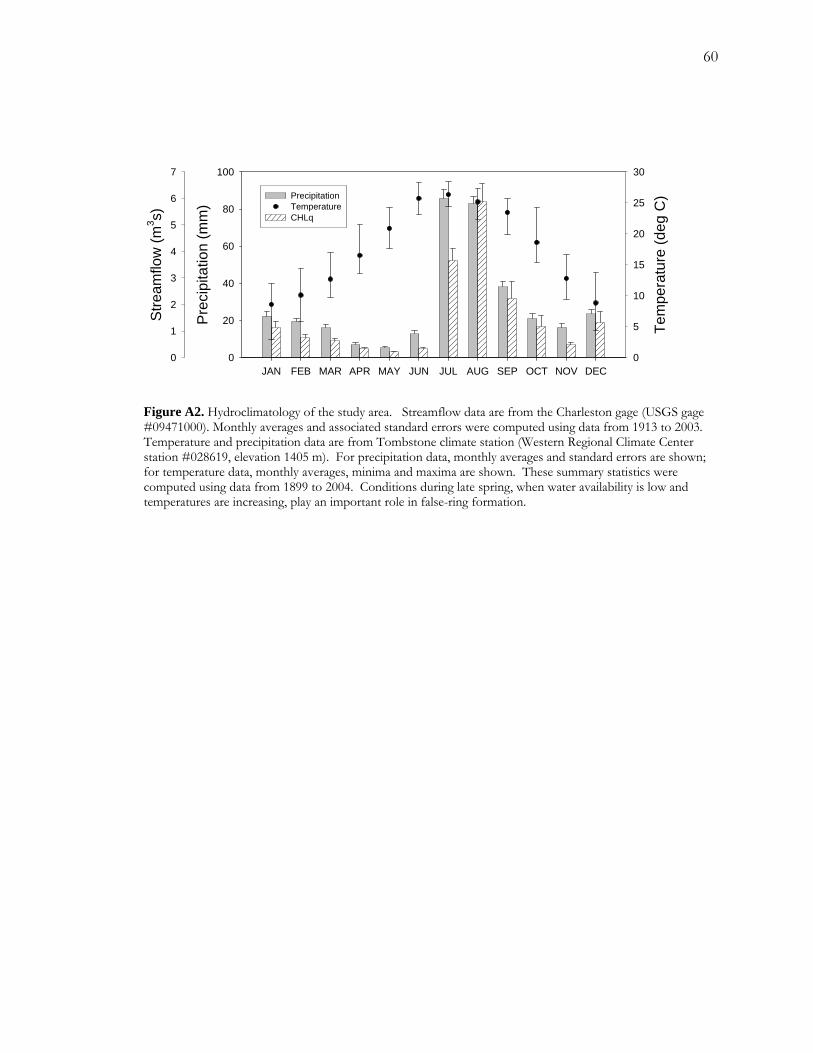
60
JAN FEB MAR APR MAY JUN JUL AUG SEP OCT NOV DEC
Pre
cipi
tatio
n (m
m)
0
20
40
60
80
100
Tem
pera
ture
(deg
C)
0
5
10
15
20
25
30S
tream
flow
(m3 s)
0
1
2
3
4
5
6
7
PrecipitationTemperatureCHLq
Figure A2. Hydroclimatology of the study area. Streamflow data are from the Charleston gage (USGS gage #09471000). Monthly averages and associated standard errors were computed using data from 1913 to 2003. Temperature and precipitation data are from Tombstone climate station (Western Regional Climate Center station #028619, elevation 1405 m). For precipitation data, monthly averages and standard errors are shown; for temperature data, monthly averages, minima and maxima are shown. These summary statistics were computed using data from 1899 to 2004. Conditions during late spring, when water availability is low and temperatures are increasing, play an important role in false-ring formation.
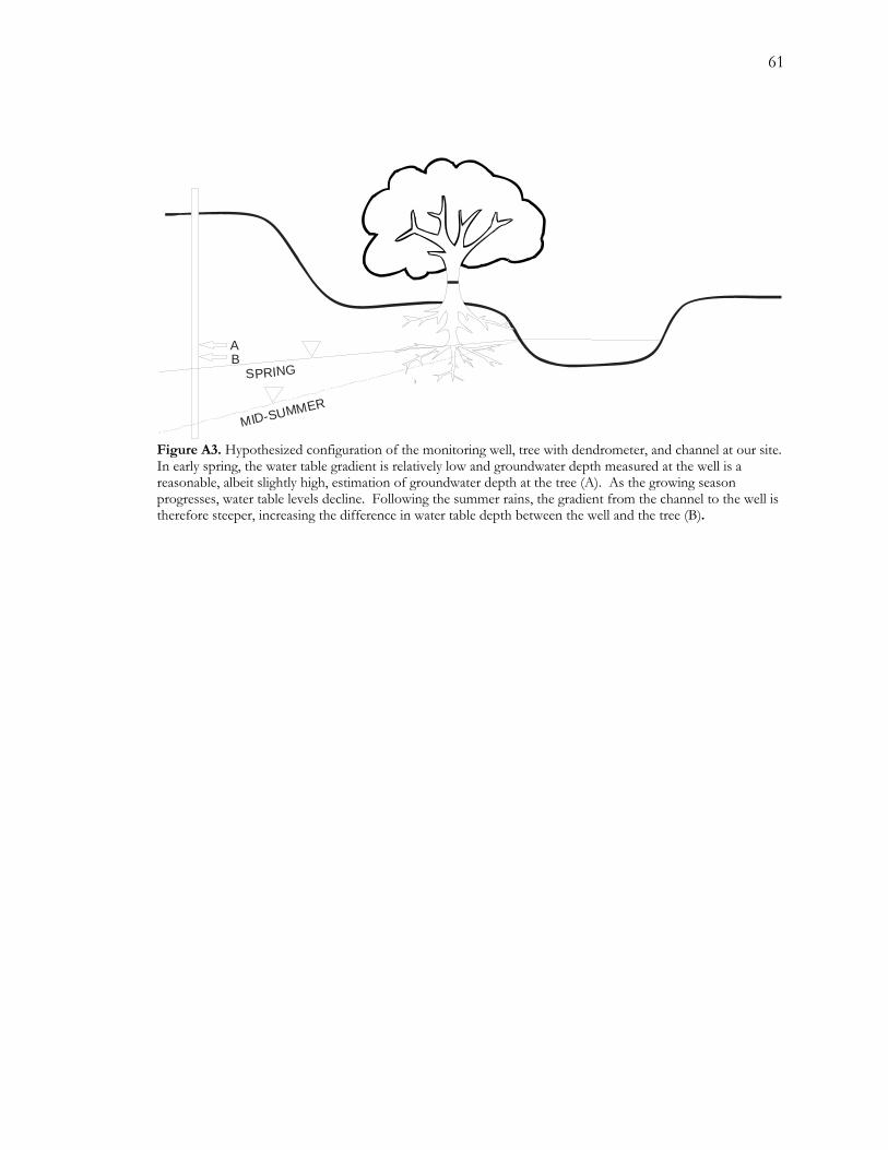
61
AB
SPRING
MID-SUMMER
Figure A3. Hypothesized configuration of the monitoring well, tree with dendrometer, and channel at our site. In early spring, the water table gradient is relatively low and groundwater depth measured at the well is a reasonable, albeit slightly high, estimation of groundwater depth at the tree (A). As the growing season progresses, water table levels decline. Following the summer rains, the gradient from the channel to the well is therefore steeper, increasing the difference in water table depth between the well and the tree (B).
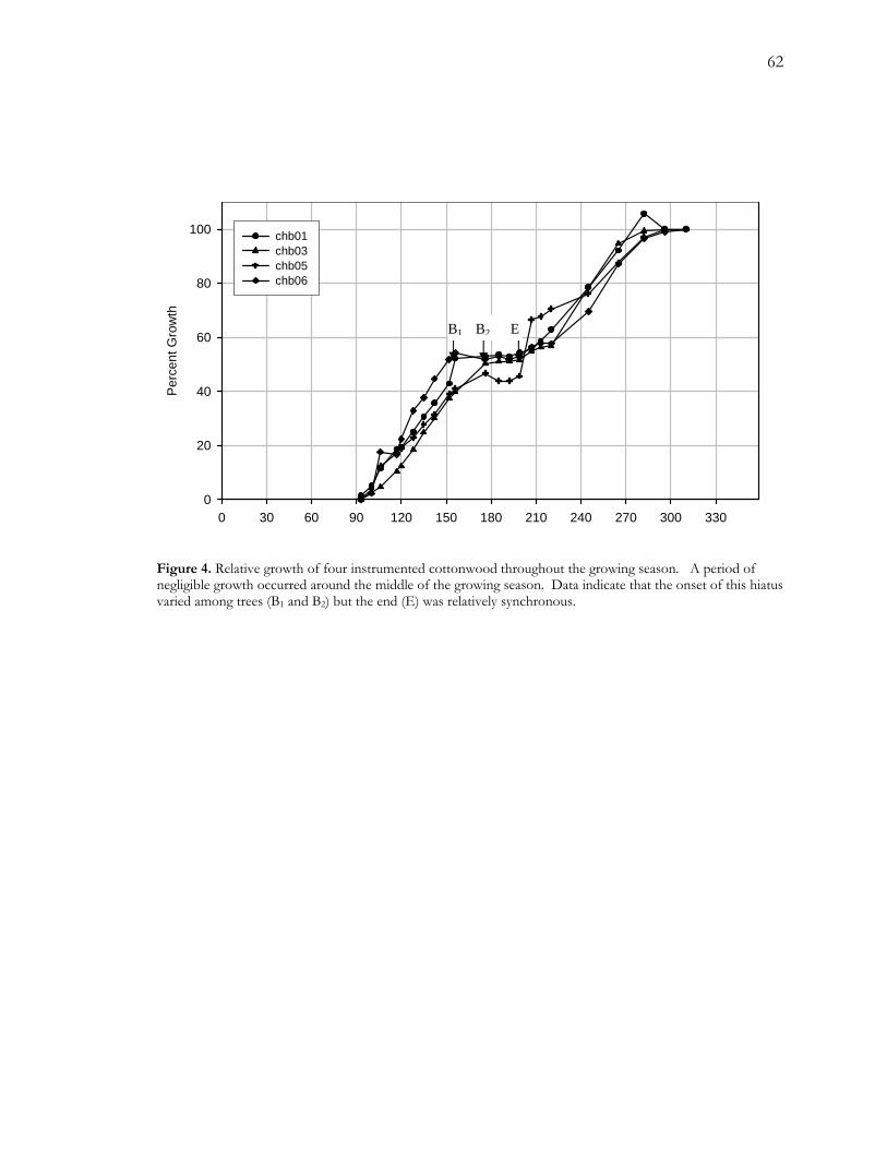
62
0 30 60 90 120 150 180 210 240 270 300 330
Per
cent
Gro
wth
0
20
40
60
80
100 chb01 chb03 chb05 chb06
BB1 B2 E
Figure 4. Relative growth of four instrumented cottonwood throughout the growing season. A period of negligible growth occurred around the middle of the growing season. Data indicate that the onset of this hiatus varied among trees (B1 and BB2) but the end (E) was relatively synchronous.
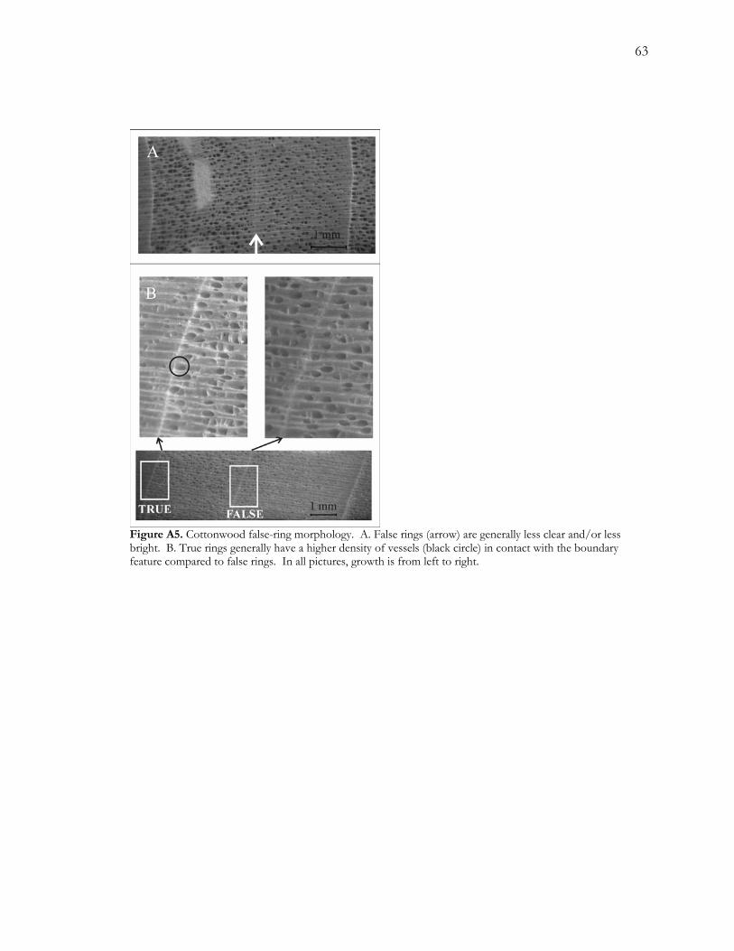
63
Figure A5. Cottonwood false-ring morphology. A. False rings (arrow) are generally less clear and/or less bright. B. True rings generally have a higher density of vessels (black circle) in contact with the boundary feature compared to false rings. In all pictures, growth is from left to right.
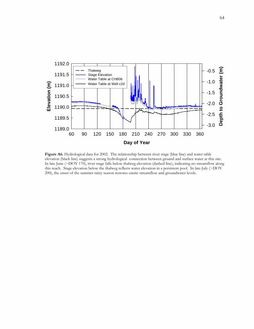
64
Day of Year
60 90 120 150 180 210 240 270 300 330 360
Elev
atio
n (m
)
1189.0
1189.5
1190.0
1190.5
1191.0
1191.5
1192.0
Dep
th to
Gro
undw
ater
(m)
-3.0
-2.5
-2.0
-1.5
-1.0
-0.5ThalwegStage ElevationWater Table at CHB06Water Table at Well c2d
Figure A6. Hydrological data for 2002. The relationship between river stage (blue line) and water table elevation (black line) suggests a strong hydrological connection between ground and surface water at this site. In late June (~DOY 170), river stage falls below thalweg elevation (dashed line), indicating no streamflow along this reach. Stage elevation below the thalweg reflects water elevation in a persistent pool. In late-July (~DOY 200), the onset of the summer rainy season restores onsite streamflow and groundwater levels.
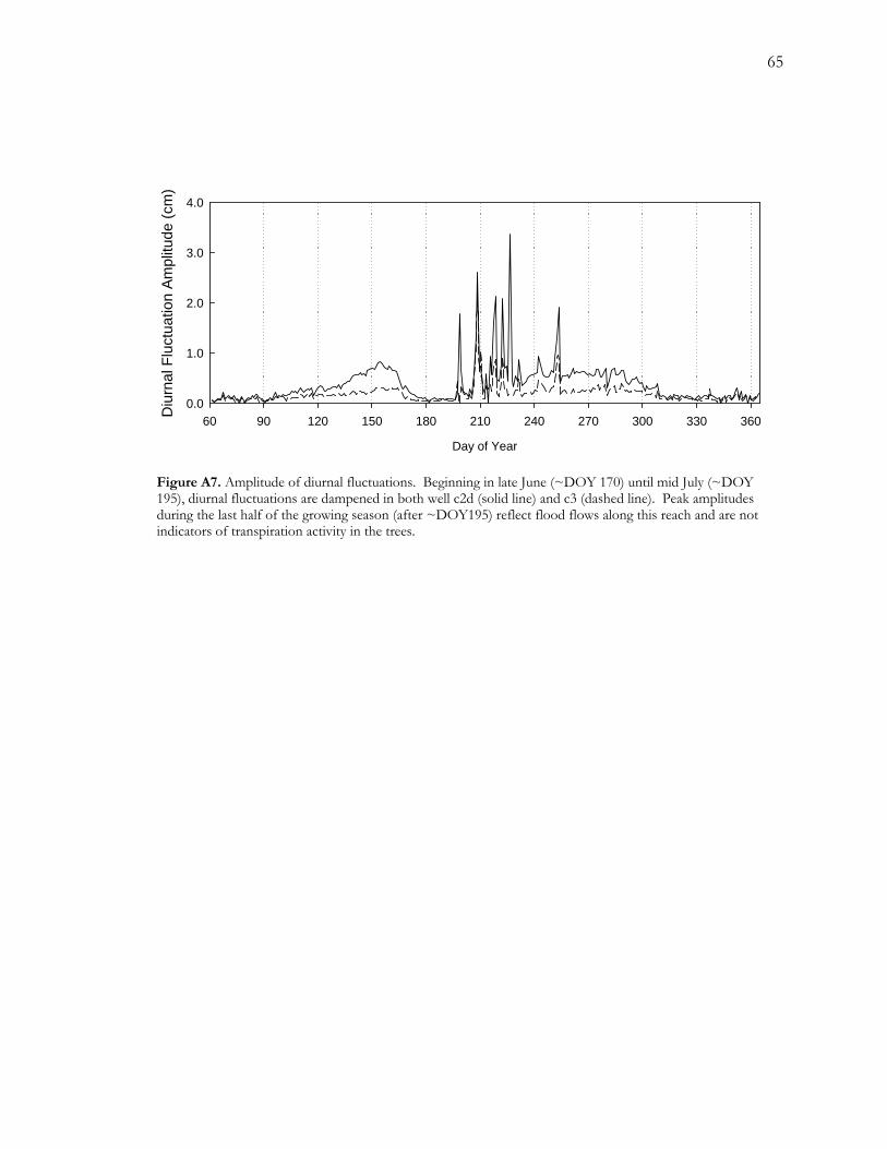
65
Day of Year
60 90 120 150 180 210 240 270 300 330 360Diu
rnal
Flu
ctua
tion
Ampl
itude
(cm
)
0.0
1.0
2.0
3.0
4.0
Figure A7. Amplitude of diurnal fluctuations. Beginning in late June (~DOY 170) until mid July (~DOY 195), diurnal fluctuations are dampened in both well c2d (solid line) and c3 (dashed line). Peak amplitudes during the last half of the growing season (after ~DOY195) reflect flood flows along this reach and are not indicators of transpiration activity in the trees.
66
A.9 Figure Captions
Figure A1. Area and site maps. The San Pedro River is located in southeastern Arizona. It
flows northward into the Gila River. We fitted four cottonwood trees ( ) with
dendrometer bands. Hydrological data was collected with groundwater monitoring wells
( ) and a (+).
Figure A2. Hydroclimatology of the study area. Streamflow data are from the Charleston
gage (USGS gage #09471000). Monthly averages and associated standard errors were
computed using data from 1913 to 2003. Temperature and precipitation data are from
Tombstone climate station (Western Regional Climate Center station #028619, elevation
1405 m). For precipitation data, monthly averages and standard errors are shown; for
temperature data, monthly averages, minima and maxima are shown. These summary
statistics were computed using data from 1899 to 2004. Conditions during late spring, when
water availability is low and temperatures are increasing, play an important role in false-ring
formation.
Figure A3. Hypothesized configuration of the monitoring well, tree with dendrometer, and
channel at our site. In early spring, the water table gradient is relatively low and groundwater
depth measured at the well is a reasonable, albeit slightly high, estimation of groundwater
depth at the tree (A). As the growing season progresses, water table levels decline.
Following the summer rains, the gradient from the channel to the well is therefore steeper,
increasing the difference in water table depth between the well and the tree (B).
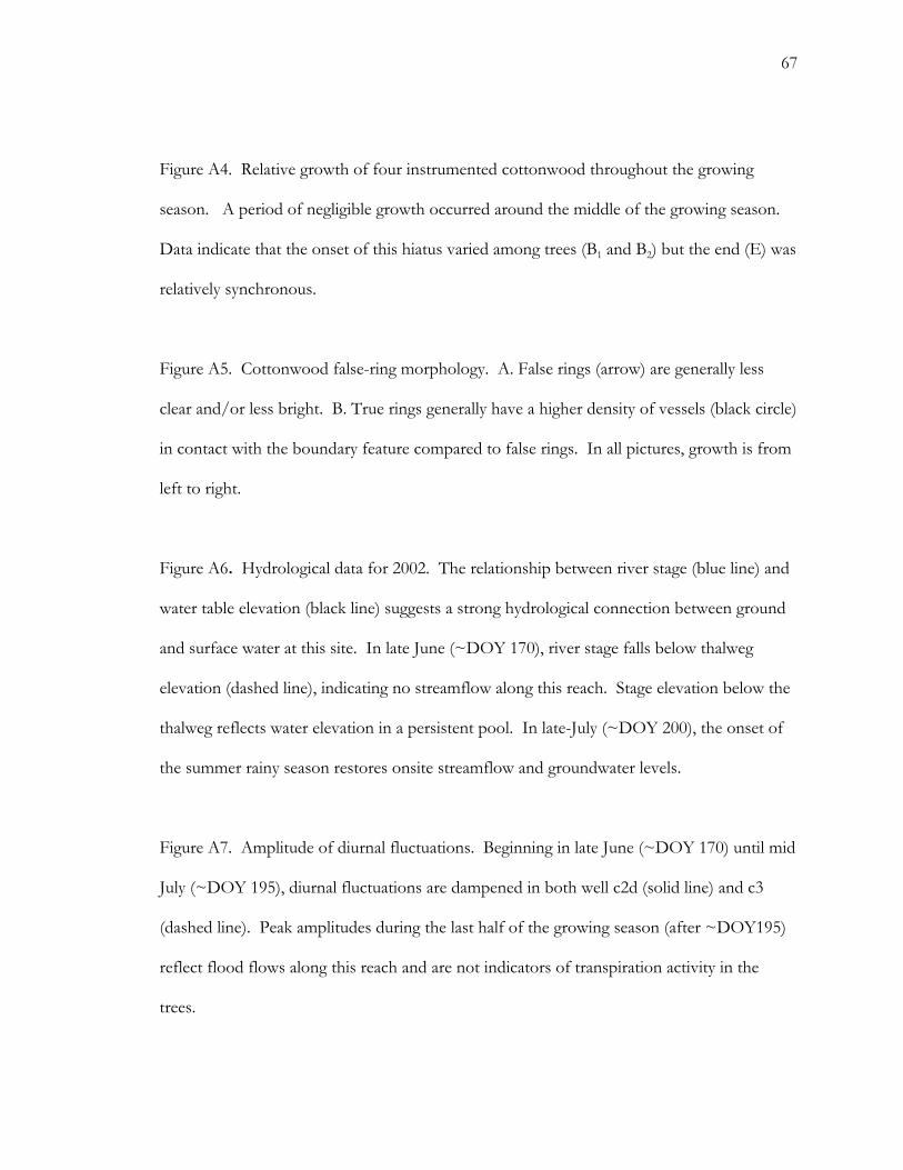
67
Figure A4. Relative growth of four instrumented cottonwood throughout the growing
season. A period of negligible growth occurred around the middle of the growing season.
Data indicate that the onset of this hiatus varied among trees (B1 and B2) but the end (E) was
relatively synchronous.
Figure A5. Cottonwood false-ring morphology. A. False rings (arrow) are generally less
clear and/or less bright. B. True rings generally have a higher density of vessels (black circle)
in contact with the boundary feature compared to false rings. In all pictures, growth is from
left to right.
Figure A6. Hydrological data for 2002. The relationship between river stage (blue line) and
water table elevation (black line) suggests a strong hydrological connection between ground
and surface water at this site. In late June (~DOY 170), river stage falls below thalweg
elevation (dashed line), indicating no streamflow along this reach. Stage elevation below the
thalweg reflects water elevation in a persistent pool. In late-July (~DOY 200), the onset of
the summer rainy season restores onsite streamflow and groundwater levels.
Figure A7. Amplitude of diurnal fluctuations. Beginning in late June (~DOY 170) until mid
July (~DOY 195), diurnal fluctuations are dampened in both well c2d (solid line) and c3
(dashed line). Peak amplitudes during the last half of the growing season (after ~DOY195)
reflect flood flows along this reach and are not indicators of transpiration activity in the
trees.

68
APPENDIX B: FALSE-RING RESPONSE IN COTTONWOOD AND WILLOW TO ARTIFICIAL DROUGHT
Kiyomi A. Morino and Edward P. Glenn
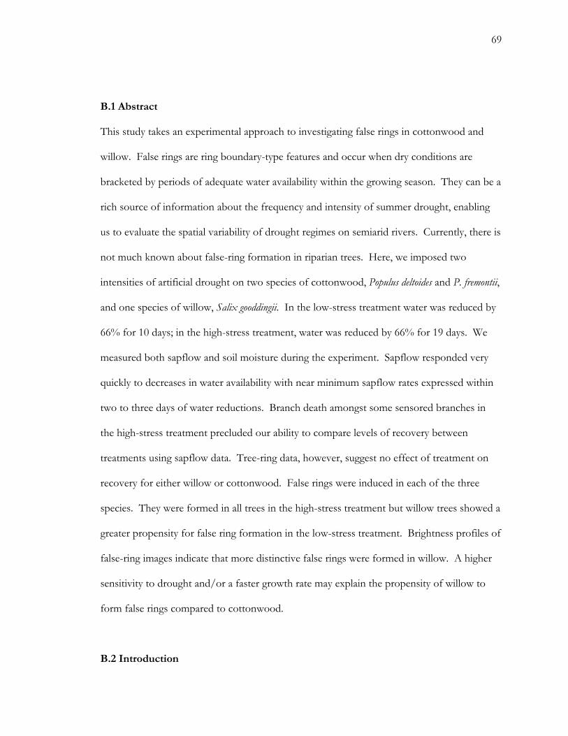
69
B.1 Abstract
This study takes an experimental approach to investigating false rings in cottonwood and
willow. False rings are ring boundary-type features and occur when dry conditions are
bracketed by periods of adequate water availability within the growing season. They can be a
rich source of information about the frequency and intensity of summer drought, enabling
us to evaluate the spatial variability of drought regimes on semiarid rivers. Currently, there is
not much known about false-ring formation in riparian trees. Here, we imposed two
intensities of artificial drought on two species of cottonwood, Populus deltoides and P. fremontii,
and one species of willow, Salix gooddingii. In the low-stress treatment water was reduced by
66% for 10 days; in the high-stress treatment, water was reduced by 66% for 19 days. We
measured both sapflow and soil moisture during the experiment. Sapflow responded very
quickly to decreases in water availability with near minimum sapflow rates expressed within
two to three days of water reductions. Branch death amongst some sensored branches in
the high-stress treatment precluded our ability to compare levels of recovery between
treatments using sapflow data. Tree-ring data, however, suggest no effect of treatment on
recovery for either willow or cottonwood. False rings were induced in each of the three
species. They were formed in all trees in the high-stress treatment but willow trees showed a
greater propensity for false ring formation in the low-stress treatment. Brightness profiles of
false-ring images indicate that more distinctive false rings were formed in willow. A higher
sensitivity to drought and/or a faster growth rate may explain the propensity of willow to
form false rings compared to cottonwood.
B.2 Introduction
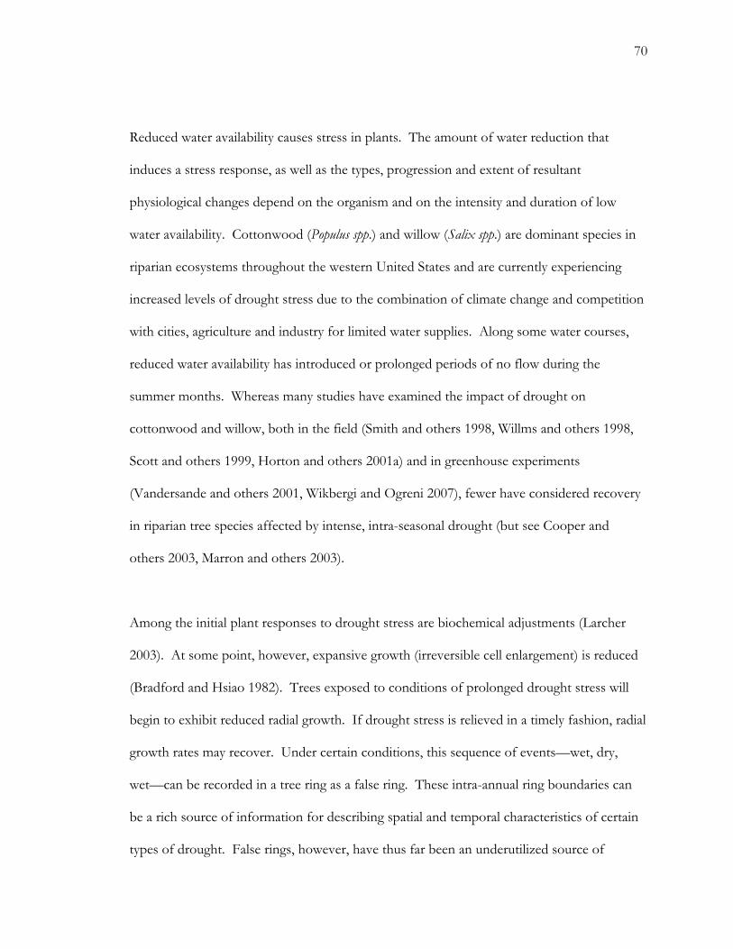
70
Reduced water availability causes stress in plants. The amount of water reduction that
induces a stress response, as well as the types, progression and extent of resultant
physiological changes depend on the organism and on the intensity and duration of low
water availability. Cottonwood (Populus spp.) and willow (Salix spp.) are dominant species in
riparian ecosystems throughout the western United States and are currently experiencing
increased levels of drought stress due to the combination of climate change and competition
with cities, agriculture and industry for limited water supplies. Along some water courses,
reduced water availability has introduced or prolonged periods of no flow during the
summer months. Whereas many studies have examined the impact of drought on
cottonwood and willow, both in the field (Smith and others 1998, Willms and others 1998,
Scott and others 1999, Horton and others 2001a) and in greenhouse experiments
(Vandersande and others 2001, Wikbergi and Ogreni 2007), fewer have considered recovery
in riparian tree species affected by intense, intra-seasonal drought (but see Cooper and
others 2003, Marron and others 2003).
Among the initial plant responses to drought stress are biochemical adjustments (Larcher
2003). At some point, however, expansive growth (irreversible cell enlargement) is reduced
(Bradford and Hsiao 1982). Trees exposed to conditions of prolonged drought stress will
begin to exhibit reduced radial growth. If drought stress is relieved in a timely fashion, radial
growth rates may recover. Under certain conditions, this sequence of events—wet, dry,
wet—can be recorded in a tree ring as a false ring. These intra-annual ring boundaries can
be a rich source of information for describing spatial and temporal characteristics of certain
types of drought. False rings, however, have thus far been an underutilized source of
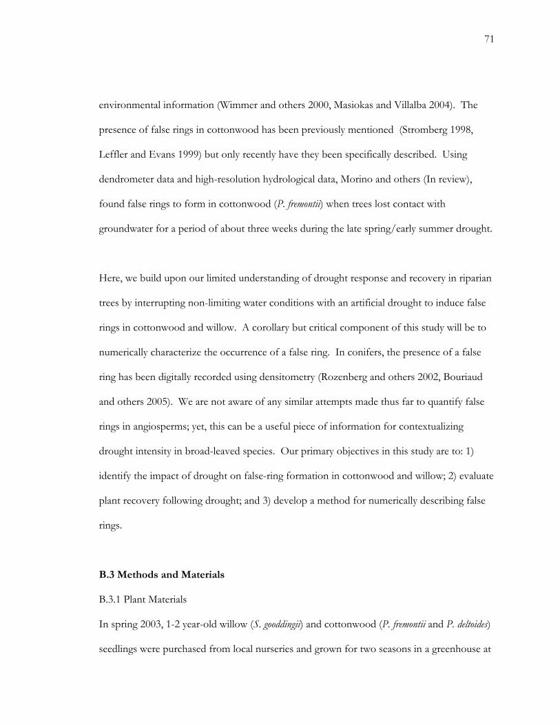
71
environmental information (Wimmer and others 2000, Masiokas and Villalba 2004). The
presence of false rings in cottonwood has been previously mentioned (Stromberg 1998,
Leffler and Evans 1999) but only recently have they been specifically described. Using
dendrometer data and high-resolution hydrological data, Morino and others (In review),
found false rings to form in cottonwood (P. fremontii) when trees lost contact with
groundwater for a period of about three weeks during the late spring/early summer drought.
Here, we build upon our limited understanding of drought response and recovery in riparian
trees by interrupting non-limiting water conditions with an artificial drought to induce false
rings in cottonwood and willow. A corollary but critical component of this study will be to
numerically characterize the occurrence of a false ring. In conifers, the presence of a false
ring has been digitally recorded using densitometry (Rozenberg and others 2002, Bouriaud
and others 2005). We are not aware of any similar attempts made thus far to quantify false
rings in angiosperms; yet, this can be a useful piece of information for contextualizing
drought intensity in broad-leaved species. Our primary objectives in this study are to: 1)
identify the impact of drought on false-ring formation in cottonwood and willow; 2) evaluate
plant recovery following drought; and 3) develop a method for numerically describing false
rings.
B.3 Methods and Materials
B.3.1 Plant Materials
In spring 2003, 1-2 year-old willow (S. gooddingii) and cottonwood (P. fremontii and P. deltoides)
seedlings were purchased from local nurseries and grown for two seasons in a greenhouse at

72
The University of Arizona’s Environmental Research Laboratory (ERL), located at the
Tucson International Airport. In 2005, twenty saplings, 10 willow and 10 cottonwood, were
transplanted to an outdoor plot on the ERL premises (Figure B1). A drip emitter irrigation
system was constructed to supply each tree with water at a rate of 2 gal/hour. Water was
supplied for 3 hours each day, yielding a total of 18 gal/day/tree. In 2006, when our
experiment was conducted, cottonwood had reached heights between approximately 4.5 and
6 m; and willows had grown to heights between approximately 3 and 5 m.
B.3.2 Soil Moisture
Soil moisture was measured using a neutron probe. A single probe port, approximately 2 m
(six feet) deep, was excavated near the base of each tree. The neutron probe utilizes
radioactivity to measure soil moisture. Fast neutrons are emitted from the probe as a result
of alpha decay. When fast neutrons collide with the hydrogen nuclei of a water molecule,
their speed is greatly reduced. The neutron probe then counts the number of slow neutrons
within a sampling sphere; this number effectively represents the number of water molecules
within that sphere. To determine actual soil moisture for a site, the probe is calibrated by
obtaining counts for soil samples with known amounts of moisture.
B.3.3 Sapflow
We measured sapflow rates to evaluate tree response to changes in water availability. Two
heat balance sapflow sensors were installed on separate branches on each tree. In the heat
balance approach to measure sapflow (Sakuratani 1981, Baker and van Bavel 1987), a
constant (and known) amount of heat is applied to a small diameter branch. Heat dissipates

73
either by convection or conduction. Convective losses involve the vertical transfer heat to
the surrounding air, as well as heat transported by the sap; conductive losses involve lateral
transfers of heat via the woody material of the branch. Using sapflow sensors designed
following Kjelgaard and others (1997), we were able to directly measure vertical heat transfer
(branch to air) and conductive losses via the wood. Convective losses of heat to sapflow
(Qf) were then computed as follows:
QH – (Qrad + Qup +Qdn) = Qf (1)
where QH is a known amount of heat applied to the branch; Qrad is heat lost to the
surrounding air; and, Qup and Qdn are measurements of heat lost to the wood by conduction
above and below the heated branch segment. Outputs from the gauges were recorded
continuously by an automatic data logger.
The heat balance component of sapflow (Qf) is converted to mass flow (S) as follows:
S = 3600Qf /4.19δTup-dn (2)
where S is in g/hr; 4.19 is the specific heat of liquid water; 3600 is the number of seconds in
an hour; and δTup-dn is the difference in temperature of the wood above and below the
heated segment. We standardized S using the cross-sectional area of the branch. Sap
velocity is therefore a measure of mass sapflow per conducting area (Schaeffer and others
2000).
B.3.4 Stress Treatments
Trees were randomly selected to belong to either the Control, Low-Stress or High-Stress
Groups (Figure B1). Each tree was supplied water by three 2 gal/hr emitters operating for
74
three hours each day. Water supply was reduced by plugging two of three emitters for a
specified number of days, depending on treatment. In the Control Group, no emitters were
plugged. Control trees received 18 gal/day. In the low-stress treatment, trees received 6
gal/day for 10 days; whereas, in the high-stress treatment, trees received 6 gal/day for 19
days. At the end of each respective stress period, water supply for each stress group was
increased to pre-treatment levels of 18 gal/day.
B.3.5 Tree core samples and wood analysis
At the end of the 2006 growing season, each tree was cored twice on opposite sides of the
bole, at a height of approximately 30 cm. After cores had dried, they were glued to a
wooden mount and surfaced using only a razor blade. When compared to a surface
prepared with sandpaper, we observed that smaller anatomical features were clearer on the
cut surface.
The 2006 growth increment was measured on all cores. When a false ring was present,
annual growth was measured in two increments: from the 2005/2006 ring boundary to the
false ring and from the false ring to the 2006/2007 ring boundary. For rings without false
rings, estimates of growth prior to and following experimental treatments were made by
dividing total ring width measurements in two, reflecting the mid-growing season timing of
the experiment. Full and partial ring width measurements were averaged for each core for
each tree.
75
The 2006 growth layer was captured digitally using a SPOT microscope digital camera (Color
Model 3.2.0, Diagnostic Instruments, Inc., Sterling Heights, MI) mounted on a Nikon
microscope (model SMZ-2T, Nikon Instruments, Inc., Melville, NY). Only one core per
tree was imaged because it was not uncommon for one of the two cores to have a crack
and/or other blemishes that would diminish our ability to quantify false ring presence. The
core was aligned so that ring boundaries and false rings were as close to vertical as possible.
In a few cases, a vertical orientation was not possible due to the curvature in the ring.
Digital images were then analyzed using MATLAB (Version 7.3.0, The Mathworks, Inc.,
Natick, MA).
B.3.6 Analysis
As all saplings were within 1-3 years in age of each other, no ring-width standardization was
conducted. Two–way ANOVAs, with species and treatment as factors, were conducted
separately on raw ring widths and false-ring location, measured as the percentage of annual
growth occurring up to the formation of the false ring.
To analyze false-ring images, images were first cropped to remove extraneous features, i.e.,
the core mount. In the resultant image, a brightness profile was computed by averaging the
values of cells in each column of the image. Lighter portions of the ring were digitally
represented by cells with higher grayscale values while darker portions were represented cells
with lower grayscale values. Figure B2 shows a 2006 growth ring with a false ring. All ring
boundary-type features are distinguished by a lighter color and therefore higher average
brightness values. The verticality of the boundary-type features in this particular sample is

76
optimal, rendering boundary-type features as distinctive peaks in the brightness profile.
When ring boundaries are curved, brightness peaks became flatter. For very non-vertical
boundary-type features, average brightness values can not be used to identify false rings.
Due to uneven lighting, and occasional stains on the wood, the brightness profile exhibited
trend and fluctuations not related to ring anatomical features (Figure B2). To detrend these
data we first generated a trend line by employing a Gaussian low-pass filter (filter width =
100) to the brightness profile. Brightness indices were then computed by subtracting the
value of the trend line from the average brightness values. As illustrated by Figure B2,
positive departures from zero occur along lighter layers of growth, including the false ring,
and negative departures occur where larger vessels have been formed. For subsequent
analyses, image profiles were truncated to highlight variation in brightness levels within the
2006 growing season. These data were summarized for each tree using boxplots to reflect
the distribution of brightness index values.
B.4 Results
B.4.1 Soil Moisture Profiles
Soil moisture readings were lowest at one foot for all probe ports (Figure B3). Neutron
probes are known to yield unreliable estimates of soil moisture near the ground surface
(Robinson and Dean 1993). We suspect that such low estimates are likely due to the
occurrence of aboveground volume (i.e., air) within the neutron probe sampling sphere.
Minimum soil moisture above four feet tended to be highest for the Control Group but
comparable for the Low- and High-Stress Groups (Figure B4). In contrast to the Low-
77
Stress Group, however, low levels of soil moisture in the High-Stress Group are maintained
for approximately twice as long.
The effect of low- and high-stress treatments was reflected in soil moisture profiles. For
trees in the low-stress treatment (10 days of reduced water availability), the moisture profile
dried over the first week then returned to its original moisture levels by Day 13. For trees in
the high-stress treatment, the moisture profile dries over the duration of the treatment
(approximately 3 weeks).
In the High-Stress Group, the largest decreases in soil moisture occur at depths of one, two
and three feet, suggesting that highest root densities occur at depths above three feet. In
contrast to trees in the Control and Low-Stress Group, soil moisture content for trees in the
high-stress treatment do not fluctuate much at depths of four, five and six feet. We interpret
this pattern as trees intercepting all available soil moisture before it percolates to these
depths.
B.4.2 Sapflow
Amongst Control Group trees, sap velocities in S. gooddingii and P. fremontii were similar,
fluctuating around a mean level of about 1000 mm/day (Figure B5). Data show sap velocity
in P. deltoides was consistently higher over the course of the experiment, fluctuating around a
mean of about 1750 mm/day. In both stress groups the impact of reduced water availability
was immediate and within 3-4 days, sap velocity dropped to very low levels for all three
species (Figure B5). When previous water levels were restored, however, the Low-Stress
78
Group exhibited a more immediate recovery than the High-Stress Group: one versus two
days. In addition, for P. fremontii, sapflow data suggest that recovery levels in the Low-Stress
Group resulted in sap velocities that exceeded the Control Group for the same period of
time (Figure B5).
In the high-stress treatment, sap velocities were comparable to the Low-Stress Group for the
first ten days but slowly decreased to a new minimum during the second phase of drought
(Figure B5). There was also less variability amongst trees during this period. Recovery
appeared to be lowest for S. gooddingii and P. deltoides trees exposed to the high-stress
treatment (Figure B5). These low and decreasing sap velocities following the high-stress
treatment indicate the eventual death of some of the sensored branches in these two species.
B.4.3 Annual Growth and False Rings in 2006
The average annual growth increment in 2006 was found to be significantly different
amongst species but not for the different treatments (Two-Way ANOVA, Prob>F =
0.0165). S. gooddingii had the lowest average growth (5.5 mm); P. fremontii had the highest
average growth (9.0 mm). The difference in ring width appears to be based on significant
differences in growth before formation of the false ring (Two-Way ANOVA, Prob>F =
0.0038). Differences in post-false-ring growth were not significantly affected by species,
treatment or an interaction between species and treatment. The location of the false ring
within the tree ring was also not affected by species, treatment or an interaction between
species and treatment. On average, the false ring was formed after about half of the annual
radial growth had occurred (52%; range: 28-78%).
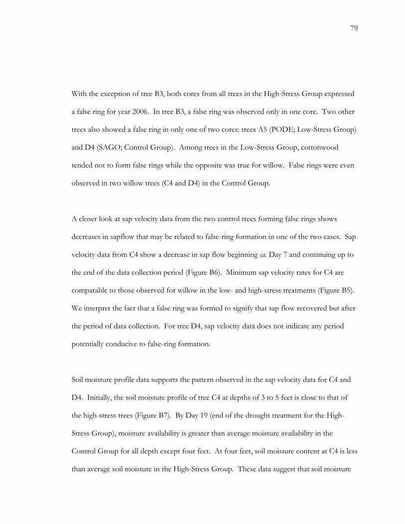
79
With the exception of tree B3, both cores from all trees in the High-Stress Group expressed
a false ring for year 2006. In tree B3, a false ring was observed only in one core. Two other
trees also showed a false ring in only one of two cores: trees A5 (PODE; Low-Stress Group)
and D4 (SAGO; Control Group). Among trees in the Low-Stress Group, cottonwood
tended not to form false rings while the opposite was true for willow. False rings were even
observed in two willow trees (C4 and D4) in the Control Group.
A closer look at sap velocity data from the two control trees forming false rings shows
decreases in sapflow that may be related to false-ring formation in one of the two cases. Sap
velocity data from C4 show a decrease in sap flow beginning ca. Day 7 and continuing up to
the end of the data collection period (Figure B6). Minimum sap velocity rates for C4 are
comparable to those observed for willow in the low- and high-stress treatments (Figure B5).
We interpret the fact that a false ring was formed to signify that sap flow recovered but after
the period of data collection. For tree D4, sap velocity data does not indicate any period
potentially conducive to false-ring formation.
Soil moisture profile data supports the pattern observed in the sap velocity data for C4 and
D4. Initially, the soil moisture profile of tree C4 at depths of 3 to 5 feet is close to that of
the high-stress trees (Figure B7). By Day 19 (end of the drought treatment for the High-
Stress Group), moisture availability is greater than average moisture availability in the
Control Group for all depth except four feet. At four feet, soil moisture content at C4 is less
than average soil moisture in the High-Stress Group. These data suggest that soil moisture

80
content at a depth of four feet plays an important role in sap flow rates for C4. For tree D4,
soil moisture is comparable to, if not greater than, average levels for the Control Group
throughout the profile over the period of data collection.
B.4.4 Digital Analysis of False Rings
Digital analysis of false rings provided the best identification of false rings in cores taken
from trees in the High-Stress Group. Boxplots for all cores taken from trees in the High-
Stress Group, except one, show positive outliers with brightness index values greater than 5
(Figure B6). The false ring observed on core PF-b3 was not represented by strong positive
outliers because of a high degree of curvature, which flattened the peak in brightness index
values. This same effect was also observed for tree SG-d4. Data suggest a difference in
false-ring expression between cottonwood and willow for trees in the high-stress treatment.
Compared to cottonwood, willow had a greater number of positive outliers (Figure B6),
indicating that false rings in willow tend to be brighter. Less distinctive false rings, such as
those observed in the Low-Stress Group (trees PD-a5, SG-a1 and SG-b2) tended to have
positive outliers but values were less than 5 (Figure B6). The mere presence of positive
outliers, however, was not enough to identify the presence of a false ring. In the Control
Group, cores PF-d1 and PF-d3 both had positive outliers but no false rings were observed
(Figure B6).
B.5 Discussion
We found that artificially imposed drought resulted in false-ring formation in cottonwood
and willow. False rings have previously been induced in conifer species. For example,
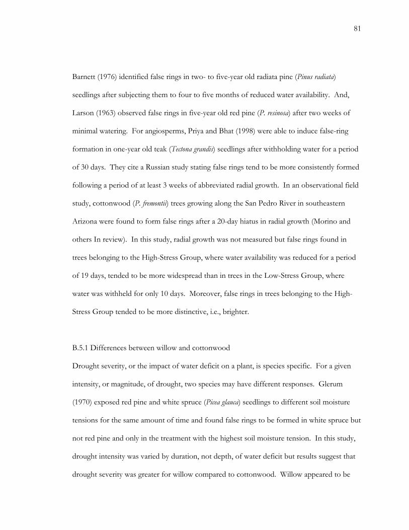
81
Barnett (1976) identified false rings in two- to five-year old radiata pine (Pinus radiata)
seedlings after subjecting them to four to five months of reduced water availability. And,
Larson (1963) observed false rings in five-year old red pine (P. resinosa) after two weeks of
minimal watering. For angiosperms, Priya and Bhat (1998) were able to induce false-ring
formation in one-year old teak (Tectona grandis) seedlings after withholding water for a period
of 30 days. They cite a Russian study stating false rings tend to be more consistently formed
following a period of at least 3 weeks of abbreviated radial growth. In an observational field
study, cottonwood (P. fremontii) trees growing along the San Pedro River in southeastern
Arizona were found to form false rings after a 20-day hiatus in radial growth (Morino and
others In review). In this study, radial growth was not measured but false rings found in
trees belonging to the High-Stress Group, where water availability was reduced for a period
of 19 days, tended to be more widespread than in trees in the Low-Stress Group, where
water was withheld for only 10 days. Moreover, false rings in trees belonging to the High-
Stress Group tended to be more distinctive, i.e., brighter.
B.5.1 Differences between willow and cottonwood
Drought severity, or the impact of water deficit on a plant, is species specific. For a given
intensity, or magnitude, of drought, two species may have different responses. Glerum
(1970) exposed red pine and white spruce (Picea glauca) seedlings to different soil moisture
tensions for the same amount of time and found false rings to be formed in white spruce but
not red pine and only in the treatment with the highest soil moisture tension. In this study,
drought intensity was varied by duration, not depth, of water deficit but results suggest that
drought severity was greater for willow compared to cottonwood. Willow appeared to be

82
more likely to form a false ring at both levels of drought stress. Additionally, willow
generally tended to have more distinct false rings than either cottonwood species at each
level of drought stress. Even two willow trees belonging to the Control Group formed false
rings. One way to evaluate drought susceptibility is to determine how vulnerable plant
xylem is to cavitation, the filling of plant cells (conducting elements) with air due to
excessive negative pressures (Tyree and others 1994, Pockman and Sperry 2000). A
comparison on P. fremontii and S. gooddingii showed no apparent differences in xylem
vulnerability (Pockman and Sperry 2000). In fact, there appear to be bigger differences in
xylem vulnerability among clones of Salix and among clones of Populus than between the two
genera (Cochard and others 2007). Nevertheless, field studies suggest that S. gooddingii is
more sensitive to drought stress than P. fremontii (Busch and Smith 1995, Horton and others
2001a, b).
Independent of xylem vulnerability, differences in growth rate may explain differences in
false-ring formation, and inferred susceptibility to drought, for cottonwood and willow.
Greenhouse studies (Nagler and others 2003) indicate that S. gooddingii grows faster than P.
fremontii. Faster growing trees tend to be more sensitive to fluctuations in water availability
(Priya and Bhat 1998, McLaughlin and others 2003, van der Werf and others 2007). The
formation of false rings in faster-growing trees has been previously recognized in Austrian
pine (P. nigra) but in the context of younger versus older trees where trees in the juvenile
growth phase had a greater propensity for false-ring formation than older trees (Wimmer
and others 2000). The apparently stronger false-ring response in willow may thus be the
result of its faster growth rate compared to cottonwood.
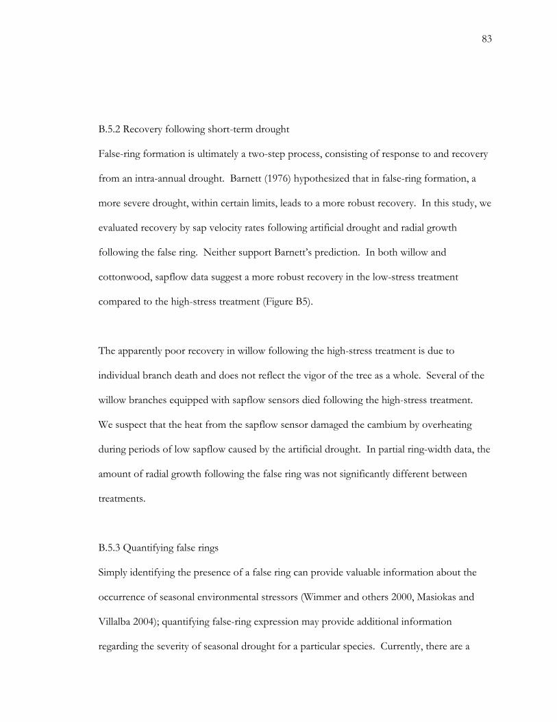
83
B.5.2 Recovery following short-term drought
False-ring formation is ultimately a two-step process, consisting of response to and recovery
from an intra-annual drought. Barnett (1976) hypothesized that in false-ring formation, a
more severe drought, within certain limits, leads to a more robust recovery. In this study, we
evaluated recovery by sap velocity rates following artificial drought and radial growth
following the false ring. Neither support Barnett’s prediction. In both willow and
cottonwood, sapflow data suggest a more robust recovery in the low-stress treatment
compared to the high-stress treatment (Figure B5).
The apparently poor recovery in willow following the high-stress treatment is due to
individual branch death and does not reflect the vigor of the tree as a whole. Several of the
willow branches equipped with sapflow sensors died following the high-stress treatment.
We suspect that the heat from the sapflow sensor damaged the cambium by overheating
during periods of low sapflow caused by the artificial drought. In partial ring-width data, the
amount of radial growth following the false ring was not significantly different between
treatments.
B.5.3 Quantifying false rings
Simply identifying the presence of a false ring can provide valuable information about the
occurrence of seasonal environmental stressors (Wimmer and others 2000, Masiokas and
Villalba 2004); quantifying false-ring expression may provide additional information
regarding the severity of seasonal drought for a particular species. Currently, there are a
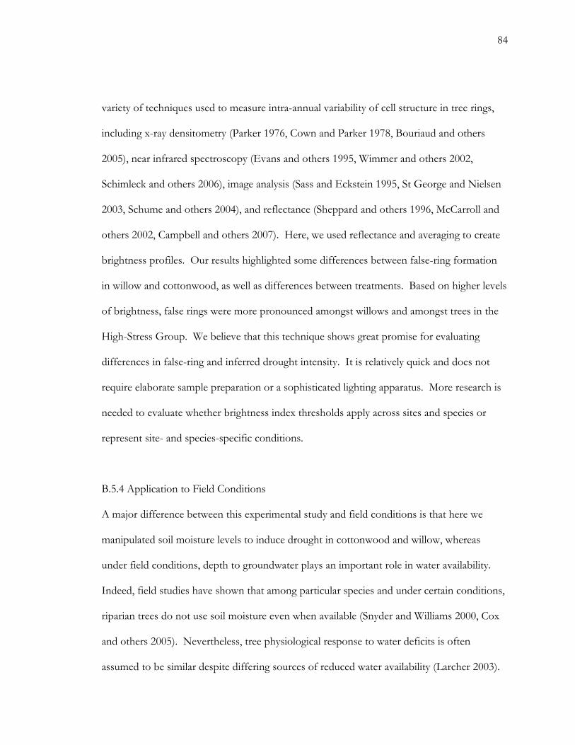
84
variety of techniques used to measure intra-annual variability of cell structure in tree rings,
including x-ray densitometry (Parker 1976, Cown and Parker 1978, Bouriaud and others
2005), near infrared spectroscopy (Evans and others 1995, Wimmer and others 2002,
Schimleck and others 2006), image analysis (Sass and Eckstein 1995, St George and Nielsen
2003, Schume and others 2004), and reflectance (Sheppard and others 1996, McCarroll and
others 2002, Campbell and others 2007). Here, we used reflectance and averaging to create
brightness profiles. Our results highlighted some differences between false-ring formation
in willow and cottonwood, as well as differences between treatments. Based on higher levels
of brightness, false rings were more pronounced amongst willows and amongst trees in the
High-Stress Group. We believe that this technique shows great promise for evaluating
differences in false-ring and inferred drought intensity. It is relatively quick and does not
require elaborate sample preparation or a sophisticated lighting apparatus. More research is
needed to evaluate whether brightness index thresholds apply across sites and species or
represent site- and species-specific conditions.
B.5.4 Application to Field Conditions
A major difference between this experimental study and field conditions is that here we
manipulated soil moisture levels to induce drought in cottonwood and willow, whereas
under field conditions, depth to groundwater plays an important role in water availability.
Indeed, field studies have shown that among particular species and under certain conditions,
riparian trees do not use soil moisture even when available (Snyder and Williams 2000, Cox
and others 2005). Nevertheless, tree physiological response to water deficits is often
assumed to be similar despite differing sources of reduced water availability (Larcher 2003).
85
A general shortcoming of controlled experiments is that the effects of only a limited number
of factors are considered. While it is incontrovertible that water availability is a key factor
influencing radial growth in cottonwood and willow, drought response may be mitigated by a
number of factors not considered in this study. For example, when these species co-occur in
more natural settings, willow, being a tree of lower stature, is often at least partially shaded
by cottonwood and therefore not exposed to the same evaporative demands. Thus, for the
same level of sub-surface water availability, drought intensity may be less for willow
compared with cottonwood. Nutrient availability is another factor we did not address. In
semiarid riparian systems, summer storms often equate to nutrient pulses (Welter and others
2005, Meixner and others 2007). Increases in nutrient availability can potentially enhance
plant recovery compared to increased levels of water availability alone (Samuelson and
others 2007). And last but not least, riparian plants are increasingly becoming exposed to
not only decreases in water availability but also increases in salinity (Busch and Smith 1995,
Pataki and others 2005), which may exacerbate plant stress response compared to decreased
levels of water availability alone.
B.6 Summary and Conclusions
A formidable strength of controlled experiments is that the effects of a specific factors can
be targeted. Whereas the results from this experiment may not be directly applicable to field
conditions, they have demonstrated a number of important points regarding the impact of
water deficits on radial growth of riparian trees. First, false rings can be induced in
cottonwood and willow by decreases in water availability for extended periods of time.
86
Whereas false rings have been observed in cottonwood (Stromberg 1998, Leffler and Evans
1999, Morino and others In review), to the best of our knowledge there is no report of them
in willow in the scientific literature. This is also the first time false rings have been
experimentally induced in either species. Second, it appears that willow is more susceptible
to false-ring formation at a given level of drought stress than cottonwood. This observation
is consistent with field studies characterizing drought vulnerability amongst riparian species
(Busch and Smith 1995, Horton and others 2001a, b). Another factor potentially
contributing to enhanced false-ring formation in willow is its elevated growth rate compared
to cottonwood. In general, faster growing plants tend to be more sensitive to fluctuations in
water availability (Priya and Bhat 1998, McLaughlin and others 2003, van der Werf and
others 2007); in particular, faster growing trees tend to be more likely to form false rings in
response to seasonal drought (Wimmer and others 2000). And lastly, false rings can be
detected in trees having diffuse-porous ring structure using image analysis techniques. We
employed a relatively simple and quick method of capturing variability in brightness over the
ring profile and were able characterize differences in false-ring intensity between low- and
high-stress treatments, as well as between willow and cottonwood.
B.7 Acknowledgements
This work was supported by a Technology and Research Initiative Fund (TRIF) Grant,
awarded to Edward P. Glenn. Bill Cable provided invaluable input regarding the sapflow
sensors. Thanks also to Fiona Jordan and Pamela Nagler for help with data collection.

87
B.8 Works Cited Baker JM, van Bavel CHM (1987) Measurement of Mass-Flow of Water in the Stems of
Herbaceous Plants. Plant Cell and Environment 10:777-782 Barnett JR (1976) Rings of collapsed cells in Pinus radiata stemwood from lysimeter-grown
trees subjected to drought. New Zealand Journal of Forestry Science 6:461-465 Bouriaud O, Leban JM, Bert D, Deleuze C (2005) Intra-annual variations in climate
influence growth and wood density of Norway spruce. Tree Physiology 25:651-660 Bradford KJ, Hsiao TC (1982) Physiological responses to moderate water stress. In: Lang
OL, Noble PS, Osmond CB, Ziegler H (eds) Encyclopedia of Plant Physiology. Springer-Verlag, Vienna, Austria, p 264-324
Busch DE, Smith SD (1995) Mechanisms associated with decline of woody species in
riparian ecosystems of the Southwestern US. Ecological Monographs 65:347-370 Campbell R, McCarroll D, Loader NJ, Grudd H, Robertson I, Jalkanen R (2007) Blue
intensity in Pinus sylvestris tree-rings: developing a new palaeoclimate proxy. Holocene 17:821-828
Cochard H, Casella E, Mencuccini M (2007) Xylem vulnerability to cavitation varies among
poplar and willow clones and correlates with yield. Tree Physiology 27:1761-1767 Cooper DJ, D'Amico DR, Scott ML (2003) Physiological and morphological response
patterns of Populus deltoides to alluvial groundwater pumping. Environmental Management 31:215-226
Cown DJ, Parker ML (1978) Comparison of annual ring density profiles in hardwoods and
softwoods by X-ray densitometry. Canadian Journal of Forest Research-Revue Canadienne De Recherche Forestiere 8:442-449
Cox G, Fischer D, Hart SC, Whitham TG (2005) Nonresponse of native cottonwood treesto
water additions during summer drought. Western North American Naturalist 65:175-185

88
Evans R, Downes G, Menz D, Stringer S (1995) Rapid measurement of variation in tracheid transverse dimensions in a radiata pine tree. Appita Journal 48:134-138
Glerum C (1970) Drought ring formation in conifers. Forest Science 16:246-248 Horton JL, Kolb TE, Hart SC (2001a) Physiological response to groundwater depth varies
among species and with river flow regulation. Ecological Applications 11:1046-1059 Horton JL, Kolb TE, Hart SC (2001b) Responses of riparian trees to interannual variation in
ground water depth in a semi-arid river basin. Plant Cell and Environment 24:293-304
Kjelgaard JF, Stockle CO, Black RA, Campbell GS (1997) Measuring sap flow with the heat
balance approach using constant and variable heat inputs. Agricultural and Forest Meteorology 85:239-250
Larcher W (2003) Physiological Plant Ecology: Ecophysiology and Stress Physiology of
Functional Groups Springer, New York Larson PR (1963) The indirect effect of drought on tracheid diameter in red pine. Forest
Science 9:52-62 Leffler AJ, Evans AS (1999) Variation in carbon isotope composition among years in the
riparian tree Populus fremontii. Oecologia 119:311-319 Marron N, Dreyer E, Boudouresque E, Delay D, Petit JM, Delmotte FM, Brignolas F (2003)
Impact of successive drought and re-watering cycles on growth and specific leaf area of two Populus x canadensis (Moench) clones, 'Dorskamp' and 'Luisa Avanzo'. Tree Physiology 23:1225-1235
Masiokas M, Villalba R (2004) Climatic significance of intra-annual bands in the wood of
Nothofagus pumilio in southern Patagonia. Trees-Structure and Function 18:696-704
89
McCarroll D, Pettigrew E, Luckman A, Guibal F, Edouard JL (2002) Blue reflectance provides a surrogate for latewood density of high-latitude pine tree rings. Arctic Antarctic and Alpine Research 34:450-453
McLaughlin SB, Wullschleger SD, Nosal M (2003) Diurnal and seasonal changes in stem
increment and water use by yellow poplar trees in response to environmental stress. Tree Physiology 23:1125-1136
Meixner T, Huth AK, Brooks PD, Conklin MH, Grimm NB, Bales RC, Haas PA, Petti JR
(2007) Influence of shifting flow paths on nitrogen concentrations during monsoon floods, San Pedro River, Arizona. Journal of Geophysical Research-Biogeosciences 112
Morino KA, Scott RL, Glenn E, Meko DM (In review) Tree-growth response to zero-flow
events: Can tree rings be used to reconstruct streamflow intermittency? Environmental Management submitted
Nagler PL, Glenn EP, Thompson TL (2003) Comparison of transpiration rates among
saltcedar, cottonwood and willow trees by sap flow and canopy temperature methods. Agricultural and Forest Meteorology 116:73-89
Parker ML (1976) Improving tree-ring dating in northern Canada by X-ray densitometry.
Syesis 9:163-172 Pataki DE, Bush SE, Gardner P, Solomon DK, Ehleringer JR (2005) Ecohydrology in a
Colorado River riparian forest: Implications for the decline of Populus fremontii. Ecological Applications 15:1009-1018
Pockman WT, Sperry JS (2000) Vulnerability to xylem cavitation and the distribution of
Sonoran desert vegetation. American Journal of Botany 87:1287-1299 Priya PB, Bhat KM (1998) False ring formation in teak (Tectona grandis Lf) and the influence
of environmental factors. Forest Ecology and Management 108:215-222 Robinson M, Dean TJ (1993) Measurement of near-surface soil-water content using a
capacitance probe. Hydrological Processes 7:77-86
90
Rozenberg P, Van Loo J, Hannrup B, Grabner M (2002) Clonal variation of wood density record of cambium reaction to water deficit in Picea abies (L.) Karst. Annals of Forest Science 59:533-540
Sakuratani T (1981) A heat balance method for measuring water flux in the stem of intact
plants. Journal of Agricultural Meteorlogy 37:9-17 Samuelson LJ, Stokes TA, Coleman MD (2007) Influence of irrigation and fertilization on
transpiration and hydraulic properties of Populus deltoides. Tree Physiology 27:765-774 Sass U, Eckstein D (1995) The variability of vessel size in beech (Fagus-Sylvatica L) and its
ecophysiological interpretation. Trees-Structure and Function 9:247-252 Schaeffer SM, Williams DG, Goodrich DC (2000) Transpiration of cottonwood/willow
forest estimated from sap flux. Agricultural and Forest Meteorology 105:257-270 Schimleck LR, Downes GM, Evans R (2006) Estimation of Eucalyptus nitens wood properties
by near infrared spectroscopy. Appita Journal 59:136-141 Schume H, Grabner M, Eckmullner O (2004) The influence of an altered groundwater
regime on vessel properties of hybrid poplar. Trees-Structure and Function 18:184-194
Scott ML, Shafroth PB, Auble GT (1999) Responses of riparian cottonwoods to alluvial
water table declines. Environmental Management 23:347-358 Sheppard PR, Graumlich LJ, Conkey LE (1996) Reflected-light image analysis of conifer tree
rings for reconstructing climate. Holocene 6:62-68 Smith SD, Devitt DA, Sala A, Cleverly JR, Busch DE (1998) Water relations of riparian
plants from warm desert regions. Wetlands 18:687-696 Snyder KA, Williams DG (2000) Water sources used by riparian trees varies among stream
types on the San Pedro River, Arizona. Agricultural and Forest Meteorology 105:227-240

91
St George S, Nielsen E (2003) Palaeoflood records for the Red River, Manitoba, Canada, derived from anatomical tree-ring signatures. Holocene 13:547-555
Stromberg J (1998) Dynamics of Fremont cottonwood (Populus fremontii) and saltcedar
(Tamarix chinensis) populations along the San Pedro River, Arizona. Journal of Arid Environments 40:133-155
Tyree MT, Kolb KJ, Rood SB, Patino S (1994) Vulnerability to drought-induced cavitation
of riparian cottonwoods in Alberta - a possible factor in the decline of the ecosystem. Tree Physiology 14:455-466
van der Werf GW, Sass-Klassen UGW, Mohren GMJ (2007) The impact of the 2003
summer drought on the intra-annual growth pattern of beech (Fagus sylvatica L.) and oak (Quercus robur L.) on a dry site in the Netherlands. Dendrochonologia 25:103-112
Vandersande MW, Glenn EP, Walworth JL (2001) Tolerance of five riparian plants from the
lower Colorado River to salinity drought and inundation. Journal of Arid Environments 49:147-159
Welter JR, Fisher SG, Grimm NB (2005) Nitrogen transport and retention in an arid land
watershed: Influence of storm characteristics on terrestrial-aquatic linkages. Biogeochemistry 76:421-440
Wikbergi J, Ogreni E (2007) Variation in drought resistance, drought acclimation and water
conservation in four willow cultivars used for biomass production. Tree Physiology 27:1339-1346
Willms J, Rood SB, Willms W, Tyree M (1998) Branch growth of riparian cottonwoods: a
hydrologically sensitive dendrochronological tool. Trees-Structure and Function 12:215-223
Wimmer R, Downes GM, Evans R (2002) High-resolution analysis of radial growth and
wood density in Eucalyptus nitens, grown under different irrigation regimes. Annals of Forest Science 59:519-524

92
Wimmer R, Strumia G, Holawe F (2000) Use of false rings in Austrian pine to reconstruct early growing season precipitation. Canadian Journal of Forest Research-Revue Canadienne De Recherche Forestiere 30:1691-1697
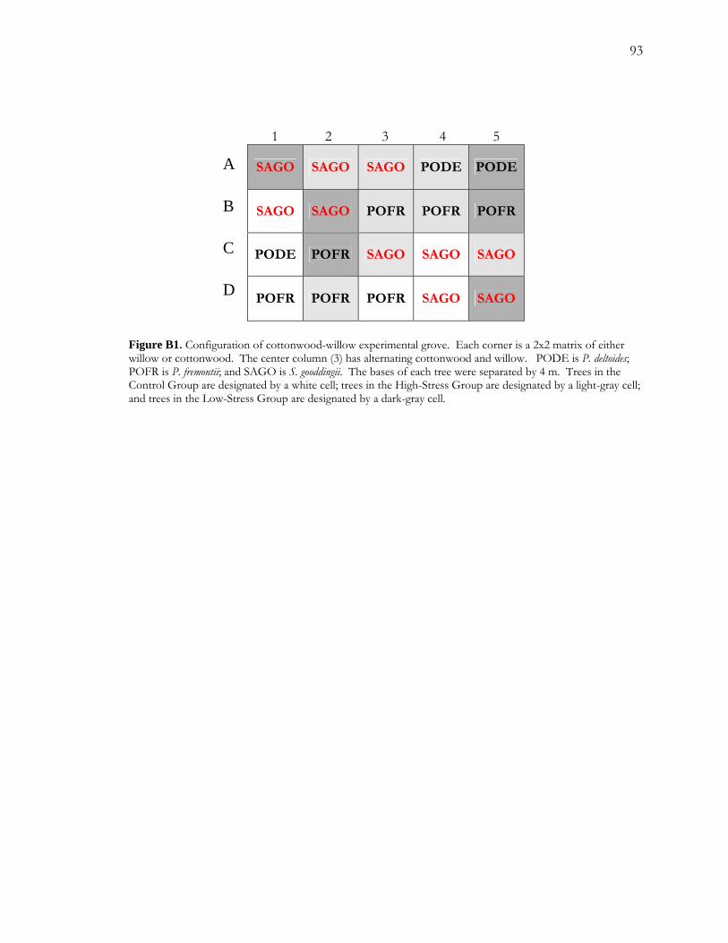
93
1 2 3 4 5 SAGO SAGO SAGO PODE PODE
SAGO SAGO POFR POFR POFR
PODE POFR SAGO SAGO SAGO
POFR POFR POFR SAGO SAGO D
C
B
A Figure B1. Configuration of cottonwood-willow experimental grove. Each corner is a 2x2 matrix of either willow or cottonwood. The center column (3) has alternating cottonwood and willow. PODE is P. deltoides; POFR is P. fremontii; and SAGO is S. gooddingii. The bases of each tree were separated by 4 m. Trees in the Control Group are designated by a white cell; trees in the High-Stress Group are designated by a light-gray cell; and trees in the Low-Stress Group are designated by a dark-gray cell.
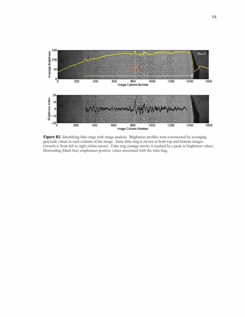
94
Figure B2. Identifying false rings with image analysis. Brightness profiles were constructed by averaging grayscale values in each column of the image. Same false ring is shown in both top and bottom images. Growth is from left to right (white arrow). False ring (orange arrow) is marked by a peak in brightness values. Detrending (black line) emphasizes positive values associated with the false ring.
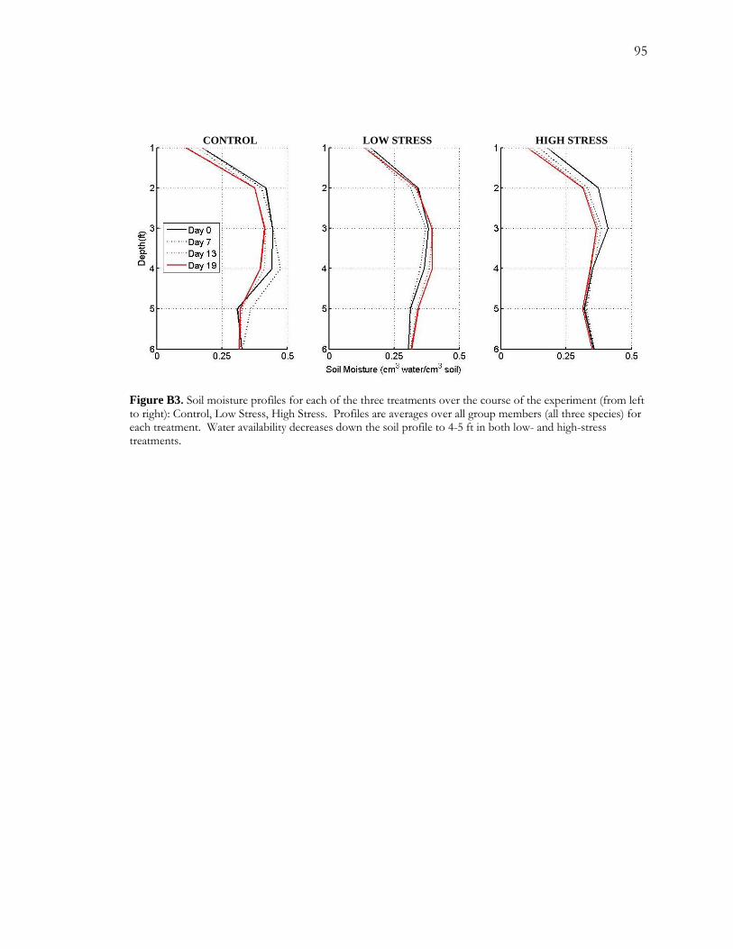
95
CONTROL LOW STRESS HIGH STRESS
Figure B3. Soil moisture profiles for each of the three treatments over the course of the experiment (from left to right): Control, Low Stress, High Stress. Profiles are averages over all group members (all three species) for each treatment. Water availability decreases down the soil profile to 4-5 ft in both low- and high-stress treatments.
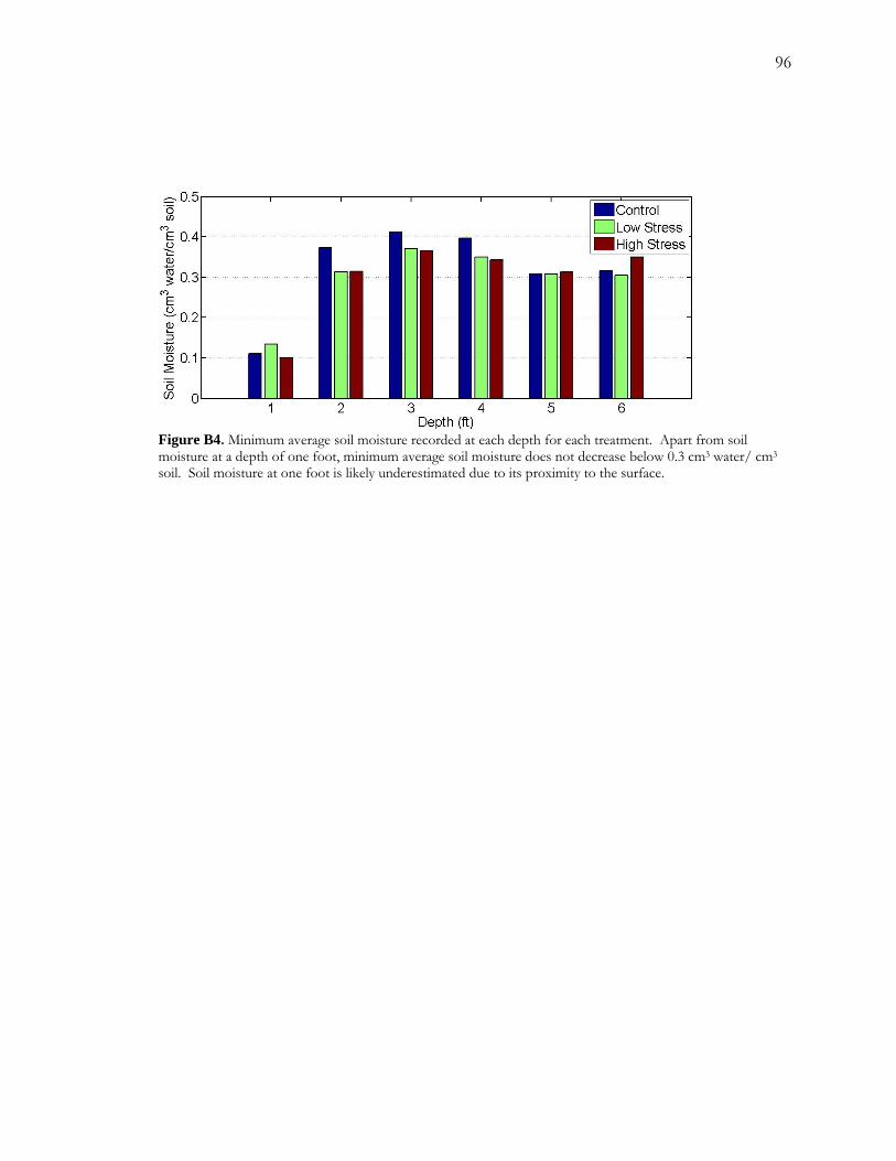
96
Figure B4. Minimum average soil moisture recorded at each depth for each treatment. Apart from soil moisture at a depth of one foot, minimum average soil moisture does not decrease below 0.3 cm3 water/ cm3 soil. Soil moisture at one foot is likely underestimated due to its proximity to the surface.
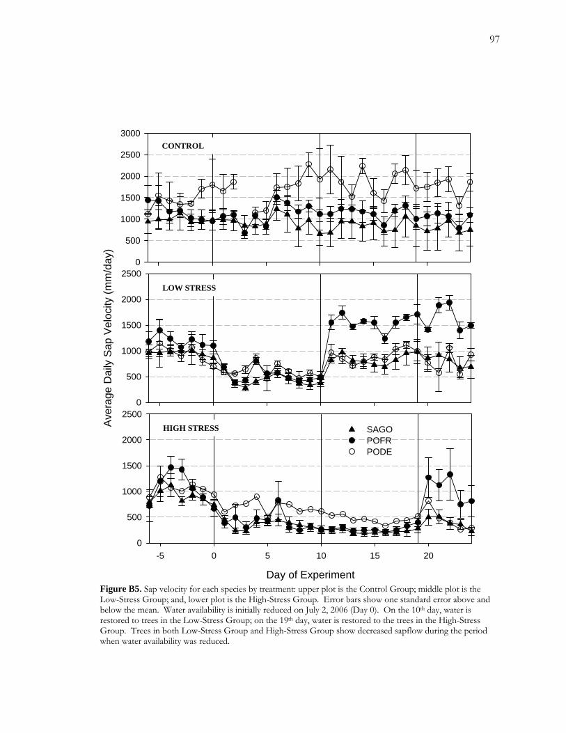
97
Figure B5. Sap velocity for each species by treatment: upper plot is the Control Group; middle plot is the Low-Stress Group; and, lower plot is the High-Stress Group. Error bars show one standard error above and below the mean. Water availability is initially reduced on July 2, 2006 (Day 0). On the 10th day, water is restored to trees in the Low-Stress Group; on the 19th day, water is restored to the trees in the High-Stress Group. Trees in both Low-Stress Group and High-Stress Group show decreased sapflow during the period when water availability was reduced.
Ave
rage
Dai
ly S
ap V
eloc
ity (m
m/d
ay)
0
500
1000
1500
2000
2500
Day of Experiment
-5 0 5 10 15 200
500
1000
1500
2000
2500
SAGOPOFRPODE
0
500
1000
1500
2000
2500
3000CONTROL
LOW STRESS
HIGH STRESS
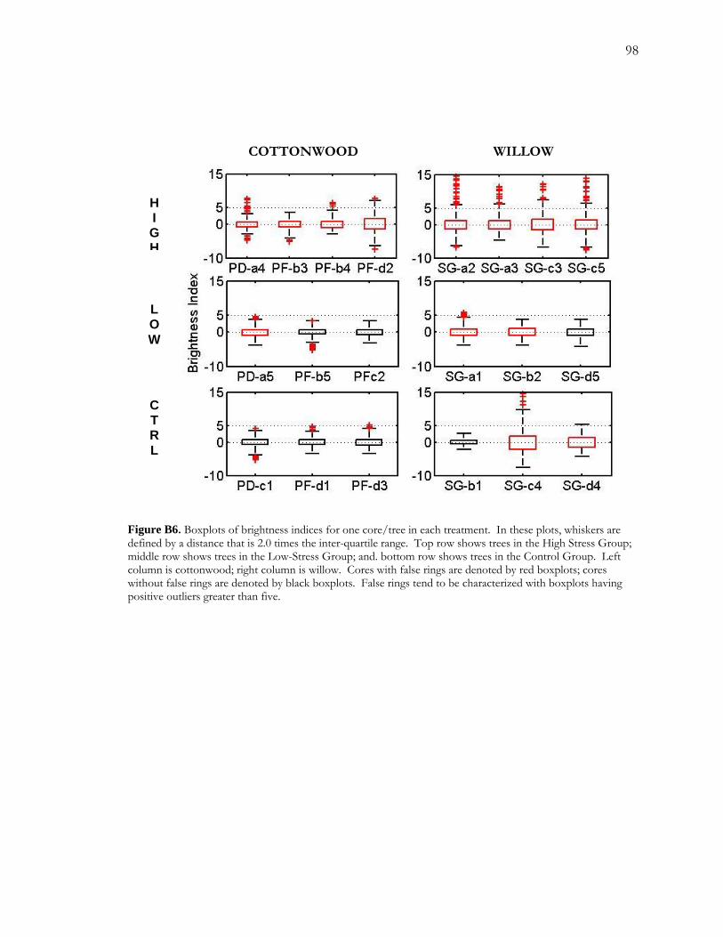
98
COTTONWOOD WILLOW
H I G H
L O W
C T R L
Figure B6. Boxplots of brightness indices for one core/tree in each treatment. In these plots, whiskers are defined by a distance that is 2.0 times the inter-quartile range. Top row shows trees in the High Stress Group; middle row shows trees in the Low-Stress Group; and. bottom row shows trees in the Control Group. Left column is cottonwood; right column is willow. Cores with false rings are denoted by red boxplots; cores without false rings are denoted by black boxplots. False rings tend to be characterized with boxplots having positive outliers greater than five.
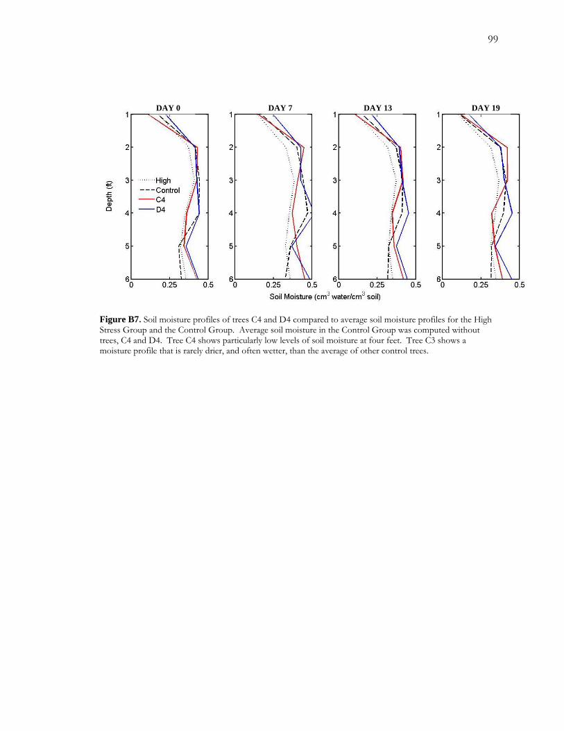
99
DAY 0 DAY 7 DAY 13 DAY 19
Figure B7. Soil moisture profiles of trees C4 and D4 compared to average soil moisture profiles for the High Stress Group and the Control Group. Average soil moisture in the Control Group was computed without trees, C4 and D4. Tree C4 shows particularly low levels of soil moisture at four feet. Tree C3 shows a moisture profile that is rarely drier, and often wetter, than the average of other control trees.

100
Day of Experiment
-5 0 5 10 15 20
Aver
age
Dal
iy
Sap
Vel
ocity
(mm
/day
)
0
500
1000
1500
2000
d4
c4
Figure B8. Average daily sap velocity for Control Group outliers, C4 (circles) and D4 (triangles). C4 shows a significant decrease in sap velocity beginning around Day 7 of the experiment and continuing past the end of the recording period. D4 does not show any apparent decrease in sap velocity.
101
B.9 Figure Captions
Figure B1. Configuration of cottonwood-willow experimental grove. Each corner is a 2x2
matrix of either willow or cottonwood. The center column (3) has alternating cottonwood
and willow. PODE is P. deltoides; POFR is P. fremontii; and SAGO is S. gooddingii. The bases
of each tree were separated by 4 m. Trees in the Control Group are designated by a white
cell; trees in the High-Stress Group are designated by a gray cell; and trees in the Low-Stress
Group are designated by a hatched cell.
Figure B2. Identifying false rings with image analysis. Brightness profiles were constructed
by averaging grayscale values in each column of the image. Same false ring is shown in both
top and bottom images. Growth is from left to right (white arrow). False ring (orange
arrow) is marked by a peak in brightness values. Detrending (black line) emphasizes positive
values associated with the false ring.
Figure B3. Soil moisture profiles for each of the three treatments over the course of the
experiment (from left to right): Control, Low Stress, High Stress. Profiles are averages over
all group members (all three species) for each treatment. Water availability decreases down
the soil profile to 4-5 ft in both low- and high-stress treatments.
Figure B4. Minimum average soil moisture recorded at each depth for each treatment. Apart
from soil moisture at a depth of one foot, minimum average soil moisture does not decrease
below 0.3 cm3 water/ cm3 soil. Soil moisture at one foot is likely underestimated due to its
proximity to the surface.
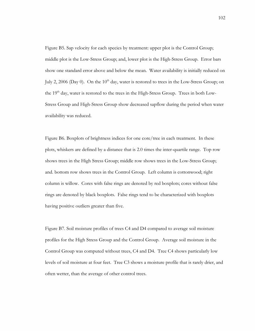
102
Figure B5. Sap velocity for each species by treatment: upper plot is the Control Group;
middle plot is the Low-Stress Group; and, lower plot is the High-Stress Group. Error bars
show one standard error above and below the mean. Water availability is initially reduced on
July 2, 2006 (Day 0). On the 10th day, water is restored to trees in the Low-Stress Group; on
the 19th day, water is restored to the trees in the High-Stress Group. Trees in both Low-
Stress Group and High-Stress Group show decreased sapflow during the period when water
availability was reduced.
Figure B6. Boxplots of brightness indices for one core/tree in each treatment. In these
plots, whiskers are defined by a distance that is 2.0 times the inter-quartile range. Top row
shows trees in the High Stress Group; middle row shows trees in the Low-Stress Group;
and. bottom row shows trees in the Control Group. Left column is cottonwood; right
column is willow. Cores with false rings are denoted by red boxplots; cores without false
rings are denoted by black boxplots. False rings tend to be characterized with boxplots
having positive outliers greater than five.
Figure B7. Soil moisture profiles of trees C4 and D4 compared to average soil moisture
profiles for the High Stress Group and the Control Group. Average soil moisture in the
Control Group was computed without trees, C4 and D4. Tree C4 shows particularly low
levels of soil moisture at four feet. Tree C3 shows a moisture profile that is rarely drier, and
often wetter, than the average of other control trees.

103
Figure B8. Average daily sap velocity for Control Group outliers, C4 (circles) and D4
(triangles). C4 shows a significant decrease in sap velocity beginning around Day 7 of the
experiment and continuing past the end of the recording period. D4 does not show any
apparent decrease in sap velocity.

104
APPENDIX C: FALSE RINGS IN COTTONWOOD (POPULUS FREMONTII): TREE-RING EVIDENCE FOR AN INTENSIFICATION OF DROUGHT IN A
SEMIARID RIVER ECOSYSTEM
Kiyomi A. Morino, David M. Meko, and Katie K. Hirschboeck

105
C1. Abstract
Drought has always been an integral component of riparian ecosystem function in semiarid
regions. Drought regimes, however, are shifting towards even drier conditions due to
climate change and increases in human water demand. It can be difficult to evaluate the
extent and impact of drier conditions on semiarid riparian ecosystems due to the paucity of
instrumental data. Here, we employ tree-rings to identify temporal shifts in drought across a
riparian landscape. Specifically, we use false-rings to characterize changes in the frequency
and intensity of seasonal drought along an approximately 10 km stretch of the San Pedro
River in southeastern Arizona. Based on the analysis of three sites positioned along a
hydrological gradient, we identified an apparent shift to drier conditions ca. 1980.
Hydrological drivers of false-ring formation appeared to vary with position along a
hydrological gradient based on streamflow permanence. No model was fit to false-ring data
from our wettest site, where streamflow was perennial. The other two sites were located
along reaches with intermittent streamflow. In the drier intermittent site, false-ring
formation appeared to be mediated by variability in recharge; whereas, in the wetter
intermittent site, false-ring formation appeared to be mediated by variability in drought
length. Sources of drought are likely related to near-stream pumping for agricultural
purposes, as well as increases in vegetation cover over the last half century.
C.2 Introduction
There are many definitions of drought but within each, it is inferred that water availability is
low relative to some previous level. Drought becomes consequential when system function
is reduced but need not always be perceived as detrimental. Some systems have developed
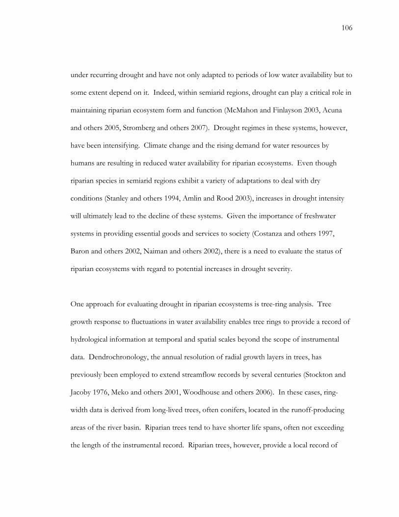
106
under recurring drought and have not only adapted to periods of low water availability but to
some extent depend on it. Indeed, within semiarid regions, drought can play a critical role in
maintaining riparian ecosystem form and function (McMahon and Finlayson 2003, Acuna
and others 2005, Stromberg and others 2007). Drought regimes in these systems, however,
have been intensifying. Climate change and the rising demand for water resources by
humans are resulting in reduced water availability for riparian ecosystems. Even though
riparian species in semiarid regions exhibit a variety of adaptations to deal with dry
conditions (Stanley and others 1994, Amlin and Rood 2003), increases in drought intensity
will ultimately lead to the decline of these systems. Given the importance of freshwater
systems in providing essential goods and services to society (Costanza and others 1997,
Baron and others 2002, Naiman and others 2002), there is a need to evaluate the status of
riparian ecosystems with regard to potential increases in drought severity.
One approach for evaluating drought in riparian ecosystems is tree-ring analysis. Tree
growth response to fluctuations in water availability enables tree rings to provide a record of
hydrological information at temporal and spatial scales beyond the scope of instrumental
data. Dendrochronology, the annual resolution of radial growth layers in trees, has
previously been employed to extend streamflow records by several centuries (Stockton and
Jacoby 1976, Meko and others 2001, Woodhouse and others 2006). In these cases, ring-
width data is derived from long-lived trees, often conifers, located in the runoff-producing
areas of the river basin. Riparian trees tend to have shorter life spans, often not exceeding
the length of the instrumental record. Riparian trees, however, provide a local record of
107
growth response to fluctuations in water availability. Thus, they can be extremely useful for
elucidating spatial patterns of water availability.
Riparian dendrochronology has been previously used to document the spatial variability of
responses to decreases in water availability due to dams (Reily and Johnson 1982, Dudek and
others 1998), diversions (Stromberg and Patten 1990), downcutting events (Scott and others
2000), and fluctuations in streamflow (Stromberg and Patten 1990, Robertson 1992,
Stromberg and Patten 1996, Dudek and others 1998, Leffler and Evans 1999). In most
cases, the relationship between tree growth and water availability is resolved on an annual
basis using either ring-width measurements or isotope data. In semi-arid regions, however,
intra-annual drought episodes can be a driving force in ecosystem structure and function.
Fluctuations of water availability at an intra-annual scale have been more difficult to
characterize using riparian tree rings. In one study, isotope analysis was conducted on sub-
divided tree rings (representing early, middle and late growth periods during each growing
season) and compared to various climatic and hydrological variables but none represented
water availability during seasonal drought (Potts and Williams 2004).
False rings, an intra-annual ring boundary, might provide a means to reconstruct seasonal
drought. The formation of false rings has been observed, as well as experimentally induced,
in many tree species, including both conifers and angiosperms (Larson 1963, Glerum 1970,
Barnett 1976, Villalba and Veblen 1996, Priya and Bhat 1998, Wimmer and others 2000,
Cherubini and others 2003, Masiokas and Villalba 2004). False rings have been identified in
cottonwood (Stromberg 1998, Leffler and Evans 1999) and have recently been described by
108
Morino and others (In review). They are usually associated with the occurrence of an
intense but relatively short period of dry conditions within the growing season. In order for
a false ring to form, the nature of the drought must be such that growth is temporarily
interrupted and resumes when moisture levels increase.
In riparian trees species, drought is largely determined by the decline of groundwater levels.
Water becomes limiting when groundwater levels decrease to elevations near, and below, the
maximum rooting depth for riparian trees. Prolonged exposure to low groundwater levels
leads to false-ring formation (Morino and others In review). A subsequent increase of
groundwater level to the rooting zone of the tree marks the end of drought and radial
growth resumes. The formation of a false ring indicates that a certain level of drought stress
has occurred. In effect, the false ring is a record of a stress “event.” As in other event-based
tree-ring studies (for example, fire history studies, e.g., Baisan and Swetnam (1990) or flood
reconstruction studies, e.g., St. George and Nielson (2003)), the proportion, or frequency of
trees, recording an event can be interpreted as a proxy for event magnitude.
The San Pedro River in south-eastern Arizona provides an ideal setting to employ the use of
cottonwood false rings to reconstruct local patterns of seasonal drought. In this river basin,
the occurrence of seasonal drought is bracketed by two periods of relatively high water
availability. In the spring, relatively high water levels reflect winter precipitation and
negligible rates of evapotranspiration during the dormant season. The progression of spring
is marked by increasingly warmer and drier conditions. Streamflow steadily decreases until it
reaches a minimum in June. The summer rainy season, in July and August, recharges

109
depleted water levels throughout the basin. In this study, our goal is twofold. We will first
characterize spatial and temporal patterns of false-ring occurrence. Then, we will use
statistical models to identify potential drivers of observed patterns.
C.3 Methods and Materials
C.3.1 Study Area
The study area is located on the San Pedro River in southeastern Arizona (Figure C1). The
San Pedro River is a low-gradient alluvial river that flows northward from its headwaters in
Mexico to its confluence with the Gila River in Arizona, USA. Our study sites were located
within the San Pedro Riparian National Conservation Area (SPRNCA). Established in 1988,
the SPRNCA covers a 50 km stretch of the river that supports a narrow ribbon of
cottonwood-willow (Populus-Salix) riparian forest. The largest urban areas in the basin and
adjacent to the SPRNCA are the city of Sierra Vista and the military post of Fort Huachuca.
The US portion of the upper basin (i.e., the Sierra Vista sub-watershed) is home to
approximately 66,000 people. Groundwater is a primary source of water for the human
population in the basin and it is also essential for the maintenance of the perennial flow and
riparian ecosystem within the SPRNCA. Some groundwater modeling studies show that
groundwater pumping has already reduced water availability in the San Pedro River
floodplain (Pool and Dickinson 2007).
C.3.2 Climate
The climate in the upper basin along the river is semiarid with a mean annual total
precipitation of around 350 mm and a mean annual average temperature of 17.5 °C (Figure
110
C2). Precipitation is typically concentrated in two parts of the year. The summer season,
spanning roughly July to September generates around 60% of annual total precipitation. The
winter season, spanning roughly December through March, accounts for much of the
remaining portion of the annual total. Perhaps the most predictable part of the annual cycle
is the dry fore-summer or pre-monsoon season from around April to July. May and June are
particularly dry, averaging 5.3 and 12.7 mm, respectively. June is also one of the hottest
months of the year averaging 25.7 °C.
C.3.3 Hydrology
The San Pedro River is an “interrupted perennial stream,” meaning that there are alternating
reaches of perennial and intermittent streamflow (Leenhouts and others 2006). Flow is
largely governed by the characteristics of the floodplain aquifer. Perennial flow generally
occurs where the volume and carrying capacity of the floodplain aquifer is low relative to
volume of discharged groundwater; reaches where this occurs are called gaining reaches.
Conversely, intermittent reaches tend to occur where the volume and carrying capacity of
the floodplain aquifer is high relative to volume of discharged groundwater; reaches where
this occurs are called losing reaches. Using isotopic analyses of surface and groundwater,
Baillie et al (2007) presented compelling evidence that streamflow in gaining reaches is
dominated by basin groundwater whereas streamflow in losing reaches is dominated by
summer floodwater recharge.
There are three primary flood seasons that influence streamflow in the San Pedro River
Basin (Hirschboeck In Press). July and August are the most active months of the year for
111
flooding, generating about 70% of annual maximum flood peaks between 1950 and 1985.
Storms and floods during this time of the year are generated by intense summer convective
rainfall. September and October, or fall, floods tend to be generated by convective rainfall,
and occasionally, by tropical storms. Winter floods are primarily generated by Pacific frontal
storms and account for only 10% of the annual maximum flood peaks in the San Pedro
River Basin. In contrast to summer floods, these floods tend to be less flashy but because
they last longer, can contribute similar, if not larger, flow volumes compared to summer
floods.
The longest-term streamflow gage on the San Pedro River is located at Charleston (Figure
C1). The record begins in 1904 but it was not until 1942 that the station was relocated to its
present site (Mac Nish and others In Press). Due to the geologic configuration of the reach
above the gage, a relatively large proportion of groundwater discharges into the stream
channel. Recent isotope studies estimate that basin groundwater currently constitutes about
half (45 ± 19%) of summer baseflow at the Charleston gaging station (Baillie et al 2007).
Analysis of streamflow data from the Charleston gage indicate that annual streamflow
decreased by 66% between 1913 and 2002 (Thomas and Pool 2006). Seasonal patterns of
streamflow indicate the largest decreases in summer (July – August) streamflow, at about
85%; whereas, winter (November – March) streamflow has only decreased about 13%.
C.3.4 Study Sites
We sampled Fremont cottonwood (Populus fremontii) in three sites along a hydrological
gradient (Figure C1). The first site, Below Charleston Gage (BCG) is located approximately
112
2.0 km downstream from the Charleston gage in a reach with perennial streamflow. The
second site, Charleston Mesquite (CHM) is located on an intermittent reach and is situated
approximately 4.5 km downstream of the Charleston gage. The third site, Fairbank (FRB) is
also located on an intermittent reach and is situated approximately 11 km downstream from
the Charleston gage. During the drier parts of the year, flow decreases from BCG to CHM
to FRB (Leenhouts and others 2006).
C.3.4 Sampling and Sample Preparation
At each site, we aimed to sample at least 20 trees. We focused on trees greater than 25 cm in
diameter. Sites contained multiple cohorts, identified by similar diameters and spatial
distribution, either in linear or clustered groups. At least five trees from each cohort were
cored two to three times at heights ranging between 0.4 and 1.8 m.
Cores were transported back to the lab, air-dried, then glued into wooden core mounts.
Cores were surfaced using only a razor blade. We did not use sandpaper as we observed it
to “smear” some of the finer anatomical features of the cottonwood tree ring. False rings
were identified according to Morino and others (In review). False rings tended to have: 1) a
less clear ring boundary, manifesting as a duller and/or less sharp boundary; 2) a lower
number of vessel elements in contact with the boundary feature; and/or 3) an apparent
lower density of vessel elements following the false ring. The expression of false rings was
variable around the circumference of the tree. If a false ring was observed on any one core
for a single tree during a particular year, that year was denoted as a false-ring year.
C.3.5 Data Analysis
113
C.3.5.1 Response Variable
In this study, the presence/absence of a false ring was the primary variable of interest.
Sample size over the period of record in each of the three sites increased over time (Figure
C3). To make comparisons both within and between sites, these data were converted to the
proportion of trees recording a false ring for a given year (Pi). The period of analysis within
each site was defined as that range of time when the number of trees in the sample set was at
least 5. Using logistic regression, the resultant chronologies of false-ring occurrence for each
site were compared to a set of potential explanatory variables.
C.3.5.2 Potential Explanatory Variables
In total, we compared false-ring data to six hydrological variables. We used streamflow data
(from the Charleston streamflow gage; USGS gage # 09471000) as a proxy for groundwater
data due to the paucity of groundwater data and the strong surface-groundwater connections
generally observed in semiarid floodplains. We limited our use of hydrological data to the
period after 1942 when the gage was re-located to its present location. We identified three
hydrological seasons based on flood occurrence: previous summer (July and August),
previous fall (September and October) and winter (previous November through March). We
also summarized data on an annual basis (previous July through June). These four variables
represent mechanisms for the provision of water at the onset and beginning of the growing
season. We found that log-transformed data provided the required linear relationship with
the response variable; therefore, mean daily streamflow was log-transformed and averaged
over the period defined by each of the four hydrological periods.

114
Seasonal drought was quantified by summing the number of days below a specified
streamflow threshold (Q<0.15 cms) during May, June and July. We theorized that the
duration of low-flow at Charleston would be related to formation of false rings in
cottonwood by indicating the period of time that streamside trees might be exposed to
drought stress prior to the onset of the summer rains. Recovery from drought was not
specifically represented in our models but is implicit in our seasonal drought variable: the
end of the observed low flow period is determined by the onset of the summer rainy season.
The sixth and final hydrological variable we compared to false-ring data was a residual mass
curve of annual streamflow. Hydrological series exhibit stronger and smoother cyclic
activity with increasing storage (Klemes 2000). Thus, a streamflow series will show higher
levels of cyclic behaviour than a precipitation series; the same applies when a groundwater
and streamflow series are compared. The physical process of storage can be represented
mathematically by summation (Salas 1992, Klemes 2000). The residual mass curve is a
running total of departures from the mean of a series and represents a storage function for
that series. In this study, we derived the residual mass curve of annual streamflow to
represent the storage dynamics of floodplain groundwater.
In addition to using hydrological variables to explain false-ring occurrence on the San Pedro
River, we also explored the role of spring temperature. Warmer springtime (average January,
February and March) temperatures since at least 1950 have been documented throughout
the western United States (Barnett and others 2008). One of the potential implications of an
earlier onset of growth for riparian vegetation is that the period of water use prior to the
115
summer rainy season is extended. Thus, plants may deplete limited water resources earlier in
the growing season thereby entering into seasonal drought earlier. A lengthened drought
would likely increase the potential for false-ring formation. Our spring temperature variable
was computed by taking the average minimum temperature for March and April.
Temperature data are from Tombstone climate station (Western Regional Climate Center
station #028619, elevation 1405 m) over the period, 1899 to 2004.
C.3.5.3 Logistic Regression Analysis
Logistic regression is a type of General Linear Model where the response variable is
measured in proportions and has a binomial distribution. The response variable is related to
a linear combination of explanatory variables using a logit (log of the odds) link. Goodness-
of-fit for a logistic regression model is evaluated using ‘deviance,’ a statistic analogous to the
sum of the squared error (SSE) in regular linear regression. In a well-fit model, the ratio of
deviance to degrees of freedom, called the dispersion coefficient, will be around unity
(Collett 2003). Ratios much larger than unity indicate overdispersion.
Logistic regression models were developed in MATLAB (Version 7.3.0, The Mathworks,
Inc., Natick, MA) using a stepwise procedure (Collett 2003). As a first filter of potential
explanatory variables, a model was fit to each variable. Variables with significant regression
coefficients (p<.10) were retained and grouped to create a full model. Full models were
reduced to final models by eliminating, one at a time, variables without significant regression
coefficients (p<.05). Correlation amongst potential explanatory variables, called
multicolinearity, can make it difficult to evaluate both the influence and significance of
116
individual variables. To avoid multicolinearity, only explanatory variables without significant
inter-correlations were grouped. High levels of correlation amongst explanatory variables
(Table C1) resulted in the formation of multiple full models for each site, where groups of 2-
4 variables were each developed into a final model. Two final models were selected for
each site based on the lowest dispersion coefficients.
C.4 Results
C.4.1 False-ring Chronologies
The longest false-ring chronology was BCG and began in 1936 (Figure C3). Hydrological
data, however, limited the period of analysis in BCG to 1942 to 2005. False-ring
chronologies for CHM and FRB were analyzed over periods of 1967 to 2004 and 1953 to
2005, respectively. BCG exhibited the lowest and FRB exhibited the highest median false-
ring proportions among the three sites, 0.08 and 0.35, respectively. CHM had the highest
maximum proportion of false rings at 0.89 in 1996 and 1997. For “strong” false-ring years
(when at least 50% of trees exhibit a false ring), the earliest event occurred in the early 1960’s
at FRB, while in BCG, the first strong false-ring year was not recorded until 2001.
In all three sites, the proportion of trees showing false rings (P) over time appears to suggest
elements of quasi-periodic behaviour. BCG shows two prominent peaks ca. 1970 and ca.
2000, and perhaps one in ca. 1980. The strongest representation of periodicity occurs in
FRB, where false-ring occurrence peaks roughly every seven years. In CHM, the early part
of the analysis period (1967 to ca. 1980) indicates relatively low levels of false-ring
occurrence. Beginning ca. 1980, however, P at CHM rapidly increases and begins to exhibit a
117
quasi-periodic character similar to FRB. Since 1980, there are four synchronous pulses of
false-ring formation in CHM and FRB. The last two pulses (ca. 1996 and ca. 2003) exhibit at
least three strong false-ring years with maximum P peaking around 90% (Figure C4).
Underlying the quasi-periodic character of P is a trend of increasing false-ring occurrence
over time in two of the three sites. The trend line in P for BCG appears to be highly
influenced by the low rate of false-ring occurrence at the beginning of the record and the
peak year of false-ring occurrence in 2001 at the end of the record (Figure C4). In fact, at
BCG false-ring frequency was on average higher in the 1970s compared to ca. 2000. For
CHM and FRB, false-ring frequency increases at a rate of 17.5% and 5% per decade,
respectively. After ca. 1980, there is a difference in the manner of false-ring frequency
increase for each site. In CHM, the increase in false-ring frequency is primarily manifested
as an increase in false-ring occurrence during episodic false-ring maxima (Figure C4). In
FRB, large fluctuations in false-ring frequency, ranging between about 10% and 75%,
characterize the false-ring record prior to ca. 1980. After ca. 1980, maximum false-ring
occurrence increases only slightly. A more substantial increase appears in the record of
minimum false-ring occurrence, yielding in the last decade a range in false-ring frequency
between about 25% and 80%.
C.4.2 Logistic Regression Models
C.4.2.1 False-ring Chronologies and Explanatory Variables
There was strong evidence suggesting a significant relationship between hydrological
variables and false-ring chronologies for two of three sites in all but one case. CHM and
118
FRB were significantly correlated to each of the seasonal streamflow variables and the
annual streamflow variable but not the mass curve for annual streamflow (Figure C5). BCG
showed very low correlations with all variables. Correlations between logit-transformed P
and potential explanatory variables indicated a weak relationship between spring temperature
and false-ring formation (Figure C5).
C.4.2.2 Final Models
Logistic regression models were developed for only two of three sites. In BCG, no
explanatory variable was found to have a significant regression coefficient. For CHM and
FRB, seven and four models were tested, respectively, but only the two models with the
lowest dispersion coefficient are reported here. All four models exhibited high levels of
overdispersion but the lower dispersion coefficient for the FRB models indicated relatively
better fits (Table C2). Models including seasonal streamflow variables performed relatively
poorly for both FRB and CHM (data not shown). In contrast, annual streamflow variables,
ANN (mean annual streamflow) and MASS (mass curve of annual streamflow), contributed
to the best fit models for each site. Also prominent is the variable representing seasonal
drought (DRY). In all cases, annual streamflow variables showed negative relationships with
P; whereas, seasonal drought showed a positive relationship.
The best model for FRB included only annual streamflow (ANN; Table C2). High
frequency (year to year) fluctuations are captured relatively well with model FRB-I, as is the
general increase in false-ring frequency after ca. 1980 (Figure C6). The mass curve of mean
annual streamflow (MASS), on its own showed a very poor fit to the data, but when

119
combined with seasonal drought, provided a reasonable model for P (Table C2, FRB-II). In
model FRB-II, high-frequency fluctuations are tracked only moderately well. In the early
1980s and 1990s, actual and predicted peak false-ring proportions tend to be offset by a year,
both preceding and post-dating the actual peak (Figure C6).
The best model for CHM included DRY and MASS (Table C2, CHM-I). High-frequency
variability is tracked moderately well, and, as was observed in model FRB-II, peak P’s in the
early 1990s are offset. Both CHM-I and CHM-II contain the variable, DRY, indicating it is
a key factor in modeling P at CHM. DRY appears to be important for capturing the
somewhat abrupt shift from low P before ca. 1980 to high but variable P after ca. 1980
(Figure C7). For comparison, we also present results from a model fit with ANN (Figure
C7). In contrast to models CHM-I and CHM-II, this model tracks high-frequency
fluctuations after ca. 1980 very well. Prior to ca. 1980, model goodness-of-fit is extremely
poor.
C.5 Discussion
Analyses of cottonwood tree rings at three sites along the San Pedro River indicate an
increasing intensity of seasonal drought over approximately the last five decades at one site
(FRB) and over the last two decades at another site (CHM). The extent and manner of
drought regime intensification varied along the hydrological gradient. Evidence of the
intensification of the drought regime at BCG, located along a reach with perennial flow, is
weak. In CHM and FRB, however, increases in false-ring frequency over the period of
120
analysis ranged between 5 and 17.5% per decade. Moreover, patterns of false-ring
occurrence suggest a regime shift ca. 1980 to drier conditions.
The shift to drier conditions ca. 1980 is expressed differently in each of the intermittent sites.
Both sites have false-ring records where false-ring occurrence alternates between maxima
and minima, suggesting a quasi-periodic behaviour of drought. In CHM, however, this
apparent periodicity begins to manifest only after ca. 1980. The high but variable occurrence
of false rings after ca. 1980 in combination with the relatively low frequency of false rings
prior to ca. 1980 produces a step-like pattern of change in false-ring occurrence. In contrast,
in FRB, there is quasi-periodicity in false-ring expression throughout the period of analysis.
Beginning ca. 1980, however, the percentage of trees producing false rings during episodes of
false-ring minima begins to increase. The intensification of the drought regime ca. 1980 is
not only indicated by the respective increases in false-ring frequencies in each of the
intermittent sites, but is also underscored by the synchronization of the high phases of false-
ring occurrence between the two sites.
We used logistic regression to identify potential factors underlying the observed false-ring
frequency patterns and thereby gain insight regarding the potential hydrological drivers of
drought on the San Pedro River. One of the challenges in modeling riparian tree growth is
the paucity of groundwater data. In natural settings, many riparian tree species respond
primarily to fluctuations in groundwater. Even cottonwood, which uses soil moisture when
it is available (Snyder and Williams 2000), becomes dependent on shallow groundwater
during seasonal drought, when groundwater is the most reliable and abundant source of
121
water. Indeed, we suspect that the quasi-periodic behavior of false-ring occurrence may
reflect groundwater dynamics as they affect fluctuations in water availability to riparian trees.
The appearance of cyclic behavior has been previously noted in hydrological time series
where storage processes are operating, such as in floodplain aquifers (Klemeš 2000).
In the absence of groundwater data, there are two approaches that have been used for
estimating the impact of water availability on tree growth. The first is to use simulated
groundwater data and compare it to tree-ring data. For example, Antonic and others (2001)
generated groundwater data from a mathematical model using the finite element method
then compared these data to basal area increments of floodplain oak (Q. robur L.) trees.
Another approach is to use streamflow data as a proxy for floodplain water table levels.
Along river reaches where the hydrological connection between surface and groundwater
levels are strong and water availability is limiting, as it can be in semiarid regions, streamflow
has proven to be an effective predictor of tree growth (eg., Stromberg and Patten 1996). In
this study, we used surface water variables but we also explored the use of a derived variable,
the residual mass curve of annual streamflow, to theoretically capture potentially important
groundwater dynamics (Klemeš 2000) that may influence riparian tree growth.
For BCG, a perennial site, no model could be fit to false-ring data, indicating that
streamflow at the Charleston gage was not representative of local water table fluctuations.
Subsurface geologic configurations can be highly complex over relatively short distances,
leading to high variability in water holding and transport characteristics within portions of
the floodplain aquifer. For example, Horton and others (2003) attributed inconsistencies

122
between plant water relations measurements and nearby groundwater monitoring wells to
high variability of substrate composition and structure.
For CHM and FRB, the intermittent sites, neither flood season variables (previous summer,
pSUM; previous fall, pFALL; and winter, WIN) nor springtime minimum temperature
entered into any of the final models, suggesting that observed changes in seasonal
streamflow on the San Pedro River (Thomas and Pool 2006) and an earlier onset of the
growing season (Barnett and others 2008) do not appear to be related to the observed
increase in drought frequency and magnitude. The three factors entering into the best-
performing final models included: log-transformed annual streamflow (ANN), the residual
mass curve of log-transformed annual streamflow (MASS), and the number of low-flow days
in May, June and July (DRY).
Despite statistically significant regression coefficients, goodness-of-fit for final models was
poor. However, relatively lower dispersion coefficients for FRB models, compared to CHM
models, suggest that streamflow at Charleston may be a better indicator of local water
availability at FRB than at CHM. Alternatively, differences in model goodness-of-fit may be
related to differences in tree response to drought at the two sites. Prior to ca. 1980, the
proportion of trees with false rings at CHM was relatively low, suggesting that water
availability was not limiting. Riparian trees establishing under conditions of unlimiting water
supply are likely to be more impacted by declines in the water table elevation than trees
establishing and developing under conditions of a limiting water supply (Albertson and
Weaver 1945, Shafroth and others 2000). In other words, the occurrence of drought at a site
123
where there had previously been none might elicit a greater response from trees than would
be predicted based on changes in water availability alone.
Even though model goodness-of-fit was low for CHM and FRB, final models provided
insight into potential hydrological factors influencing false-ring formation in cottonwood.
For instance, there is an interesting contrast in the single-variable models for CHM and
FRB. In the wetter site, CHM, length of the low-flow period (DRY) was found to be
significant; in the drier site, FRB, average level of annual streamflow prior to the onset of
seasonal drought (ANN; Table C2) was found to be significant. These two variables
represent different processes influencing groundwater fluctuations. The length of the low-
flow period (DRY) is constructed from streamflow levels during a period of the year when
runoff is minimal and discharge processes, for example, transpiration and groundwater
pumping, dominate. As a result, both streamflow and groundwater levels decrease. In
contrast, the annual streamflow variable, ANN, represents recharge processes leading to
increases in streamflow and groundwater levels. ANN was constructed to capture the major
flood seasons of the San Pedro River basin. If we hypothesize that there exists a critical
depth to groundwater (Dc), where if exceeded for a long enough period of time drought
stress occurs in streamside trees, then on this stretch of the San Pedro River false-ring
formation in trees from a wetter site appears to be more related to factors influencing the
water table decline, or discharge; whereas false-ring formation in trees from drier sites
appears to be more related to factors influencing water table increase, or recharge.
124
One of the findings of this research is an apparent increase in drought, beginning ca. 1980.
The three explanatory variables in our final models all indicate a hydrological shift in the
1980s (Figure C8). The most striking change can be observed in the residual mass curve for
annual streamflow. The steep decline beginning in the mid-1980s reflects how apparently
small declines in annual streamflow might be manifested as larger reductions in groundwater
storage. Models including the mass curve of annual flow appear to perform slightly better in
the last decade compared to models using annual streamflow as an explanatory variable for
false-ring occurrence. The shift in low flow ca. 1980 is also apparent when the distribution
of low-flow days in May, June and July is plotted over the period of analysis (Figure C9).
Since 1980, there have been many more occurrences of low flow beginning in early May;
moreover, since the mid-1990s, there have been instances of low flow beginning in April.
The duration of the low-flow period has also been extended on the back end. After ca. 1980,
low-flow periods are more likely to extend into late July.
Decreases in streamflow and a shift towards drier conditions have previously been
documented for the San Pedro River. Most recently, Thomas and Pool (2006) have
conducted extensive hydrological analyses and have described changes in the hydrological
regime at the Charleston stream gage. They found significant decreases in annual and
seasonal (except winter) streamflow between 1913 and 2002. Other hydrological decreases
included spring (April-June) and summer (July-August) low flow, decreasing by 42 and 67%,
respectively. Of all the decreases noted, however, only Fall (September-October) and July
streamflow show possible inflection points of increasing rates of decline ca. 1980 (Thomas
and Pool 2006, Figures 1&13).
125
The primary causes of streamflow decline on the San Pedro River have widely been
recognized as some combination of groundwater pumping and vegetation change (Lite and
Stromberg 2005, Thomas and Pool 2006). The drought history revealed by false-ring
chronologies highlights some intriguing associations between periods of low water
availability, as it affects streamside trees, and temporal patterns of groundwater pumping and
vegetation change. In the San Pedro River basin, groundwater serves as a primary water
source for agricultural, industrial and municipal purposes. The impact of groundwater
pumping on streamflow is related in part to the proximity of pumping activities to the
floodplain aquifer. Agricultural activities within the San Pedro River basin are generally
located in or near the floodplain and thus would be expected to have an immediate impact
on streamflow levels. Increases in groundwater extraction for agricultural purposes show
two periods of increase since ca. 1950 (Thomas and Pool 2006). The first occurred in the
mid-1960s; the second began in the early 1970s, peaked by the late 1970s and lasted until the
mid-1980s. The former overlaps closely with an early period of extended seasonal drought
observed in this study (Figures C8&C9). The timing and duration of the latter period of
high agricultural activity, however, fit less well with the shift to drier conditions ca. 1980.
Two additional, or alternative, factors may account for increased levels of seasonal drought
since 1980. First, Mexican mining activities peaked in the late 1990s (Thomas and Pool
2006). Cananea is a large copper mine located in the headwaters of the San Pedro River.
And second, between 1973 and 1986 there was an approximately 500% increase in mesquite
cover (Prosopis velutina) in the Upper San Pedro watershed (Kepner and others 2000).
Mesquite trees establish on the upper terraces of the floodplain. The deeper roots of a
126
mesquite tree could reduce streamflow by intercepting groundwater flowing into the stream
and/or by depleting groundwater levels in the floodplain aquifer. It is also possible that
recent decreases in streamflow on the San Pedro are due to decreases in the movement of
groundwater from the regional to the floodplain aquifer due to groundwater pumping for
municipal and industrial purposes (see Thomas and Pool 2006, Table 25).
C.6 Summary and Conclusions
In this study, false rings in cottonwood were used to highlight changes in the hydrological
regime. False-ring chronologies indicate that drought severity has been increasing along
some segments of the San Pedro River over the last 40 to 50 years. In addition to the
upward trend, drought severity at all three sites shows a pattern of quasi-periodicity with a
possible shift to drier conditions ca. 1980. Possible hydrological drivers of this shift include
groundwater pumping activities on or near the floodplain and changes in vegetation during
the last half of the twentieth century. The hydrological factors influencing false-ring
occurrence appear to depend on relative water availability. For drier sites, recharge appears
to be important; for wetter sites, length of drought appears to be important.
There are two related advantages of using tree-ring data to evaluate riparian ecosystems.
First, it is possible to reconstruct the hydrological regime during an earlier period. In this
study, for example, false-ring data suggest that prior to ca. 1980 water availability was not
limiting in CHM but was highly variable in FRB, suggesting that dry conditions have
episodically prevailed along some portions of the San Pedro River over the last half century.
And second, false rings provide information of water availability at a spatial scale that is
127
rarely afforded by instrumental data. Evidence from this study indicates that CHM and FRB
have been impacted by decreases in water availability whereas BCG has not. Being able to
identify which areas might be more susceptible to drought could facilitate a more efficient
realization of management actions.
One of the challenges for resources manager is to identify variables that are indicative of the
state of the ecosystem. Overstory riparian trees regulate many ecosystem processes in
semiarid regions; therefore, monitoring this functional group could be a source of important
information. This study has demonstrated that tree-ring analyses enable the detection of low
to moderately severe changes in hydrological regimes on riparian ecosystems prior to their
ecological expression. The effect of gradual increases in drought intensity will first be
manifested in tree growth. Increasing intensity will result in tree death and ultimately
changes in community composition. Having knowledge of the progression and stage of
drought, as well as the variability of ecosystem response and susceptibility over space, can
contribute to the development of management plans. For this reason, we believe that false-
ring analysis can be used to augment and compliment current efforts aimed at the
conservation of riparian ecosystems in semiarid regions.
C.7 Acknowledgements
This work was supported by a Technology and Research Initiative Fund (TRIF) Grant
awarded to Edward P. Glenn. Mike Burton and Devin Petry provided invaluable field
assistance.
128
C.8 Works Cited
Acuna V, Munoz I, Giorgi A, Omella M, Sabater F, Sabater S (2005) Drought and postdrought recovery cycles in an intermittent Mediterranean stream: structural and functional aspects. Journal of the North American Benthological Society 24:919-933
Albertson FW, Weaver JE (1945) Injury and death or recovery of trees in prairie climate.
Ecological Monographs 15:393-433 Amlin NM, Rood SB (2003) Drought stress and recovery of riparian cottonwoods due to
water table alteration along Willow Creek, Alberta. Trees-Structure and Function 17:351-358
Antonic O, Hatic D, Krian J, Bukovec D (2001) Modelling groundwater regime acceptable
for the forest survival after the building of the hydro-electric power plant. Ecological Modelling 138:277-288
Baillie MN, Hogan JF, Ekwurzel B, Wahi AK, Eastoe CJ (2007) Quantifying water sources
to a semiarid riparian ecosystem, San Pedro River, Arizona. Journal of Geophysical Research-Biogeosciences 112:S02
Baisan CH, Swetnam TW (1990) Fire History on a Desert Mountain-Range - Rincon
Mountain Wilderness, Arizona, USA. Canadian Journal of Forest Research-Revue Canadienne De Recherche Forestiere 20:1559-1569
Barnett JR (1976) Rings of collapsed cells in Pinus radiata stemwood from lysimeter-grown
trees subjected to drought. New Zealand Journal of Forestry Science 6:461-465 Barnett TP, Pierce DW, Hidalgo HG, Bonfils C, Santer BD, Das T, Bala G, Wood AW,
Nozawa T, Mirin AA, Cayan DR, Dettinger MD (2008) Human-induced changes in the hydrology of the western United States. Science 319:1080-1083
Baron JS, Poff NL, Angermeier PL, Dahm CN, Gleick PH, Hairston NG, Jackson RB,
Johnston CA, Richter BD, Steinman AD (2002) Meeting ecological and societal needs for freshwater. Ecological Applications 12:1247-1260

129
Cherubini P, Gartner BL, Tognetti R, Braker OU, Schoch W, Innes JL (2003) Identification, measurement and interpretation of tree rings in woody species from mediterranean climates. Biological Reviews 78:119-148
Collett D (2003) Modeling Binary Data, Chapman & Hall / CRC, Boca Raton Costanza R, dArge R, deGroot R, Farber S, Grasso M, Hannon B, Limburg K, Naeem S,
Oneill RV, Paruelo J, Raskin RG, Sutton P, vandenBelt M (1997) The value of the world's ecosystem services and natural capital. Nature 387:253-260
Dudek DM, McClenahen JR, Mitsch WJ (1998) Tree growth responses of Populus deltoides
and Juglans nigra to streamflow and climate in a bottomland hardwood forest in central Ohio. American Midland Naturalist 140:233-244
Glerum C (1970) Drought ring formation in conifers. Forest Science 16:246-248 Hirschboeck KK (In Press) Flood flows of the San Pedro River. In: Stromberg JC, Tellman
B (eds) Ecology and Conservation of the San Pedro River. University of Arizona Press, Tucson
Horton JL, Hart SC, Kolb TE (2003) Physiological condition and water source use of
Sonoran Desert riparian trees at the Bill Williams River, Arizona, USA. Isotopes in Environmental and Health Studies 39:69-82
Kepner WG, Watts CJ, Edmonds CM, Maingi JK, Marsh SE, Luna G (2000) Landscape
approach for detecting and evaluating change in a semiarid environment. Environmental Monitoring and Assessment 64:179-195
Klemes V (2000) Common Sense and Other Heresies, Canadian Water Resources
Association, Waterloo Larson PR (1963) The indirect effect of drought on tracheid diameter in red pine. Forest
Science 9:52-62

130
Leenhouts JM, Stromberg J, Scott RL (2006) Hydrologic requirements of and consumptive use by riparian vegetation along the San Pedro River, Arizona. U.S. Geological Survey Scientific Investigations Report 2005-5163
Leffler AJ, Evans AS (1999) Variation in carbon isotope composition among years in the
riparian tree Populus fremontii. Oecologia 119:311-319 Lite SJ, Stromberg JC (2005) Surface water and ground-water thresholds for maintaining
Populus-Salix forests, San Pedro River, Arizona. Biological Conservation 125:153-167 Mac Nish R, Baird K, Maddock T (In Press) Groundwater hydrology of the San Pedro
Basin. In: Stromberg JC, Tellman B (eds) Ecology and Conservation of the San Pedro River. University of Arizona Press, Tucson
Masiokas M, Villalba R (2004) Climatic significance of intra-annual bands in the wood of
Nothofagus pumilio in southern Patagonia. Trees-Structure and Function 18:696-704 McMahon TA, Finlayson BL (2003) Droughts and anti-droughts: the low flow hydrology of
Australian rivers. Freshwater Biology 48:1147-1160 Meko DM, Therrell MD, Baisan CH, Hughes MK (2001) Sacramento River flow
reconstructed to AD 869 from tree rings. Journal of the American Water Resources Association 37:1029-1039
Morino KA, Scott RL, Glenn E, Meko DM (In review) Tree-growth response to zero-flow
events: Can tree rings be used to reconstruct streamflow intermittency? Environmental Management submitted
Naiman RJ, Bunn SE, Nilsson C, Petts GE, Pinay G, Thompson LC (2002) Legitimizing
fluvial ecosystems as users of water: An overview. Environmental Management 30:455-467
Pool DR, Dickinson JE (2007) Ground-water flow model of the Sierra Vista Subwatershed
and Sonoran portions of the Upper San Pedro Basin, southeastern Arizona, United States, and northern Sonora, Mexico. U.S. Geological Survey Scientific Investigations Report 2006-5228
131
Potts DL, Williams DG (2004) Response of tree ring holocellulose delta C-13 to moisture availability in Populus fremontii at perennial and intermittent stream reaches. Western North American Naturalist 64:27-37
Priya PB, Bhat KM (1998) False ring formation in teak (Tectona grandis Lf) and the influence
of environmental factors. Forest Ecology and Management 108:215-222 Reily PW, Johnson WC (1982) The effects of altered hydrologic regime on tree growth along
the Missouri River in North-Dakota. Canadian Journal of Botany-Revue Canadienne De Botanique 60:2410-2423
Robertson PA (1992) Factors affecting tree growth on 3 lowland sites in southern Illinois.
American Midland Naturalist 128:218-236 Salas JD (1992) Analysis and modeling of hydrologic time series. In: Maidment DR (ed)
Handbook of Hydrology. McGraw-Hill Inc. , New York Scott ML, Lines GC, Auble GT (2000) Channel incision and patterns of cottonwood stress
and mortality along the Mojave River, California. Journal of Arid Environments 44:399-414
Shafroth PB, Stromberg JC, Patten DT (2000) Woody riparian vegetation response to
different alluvial water table regimes. Western North American Naturalist 60:66-76 Snyder KA, Williams DG (2000) Water sources used by riparian trees varies among stream
types on the San Pedro River, Arizona. Agricultural and Forest Meteorology 105:227-240
St George S, Nielsen E (2003) Palaeoflood records for the Red River, Manitoba, Canada,
derived from anatomical tree-ring signatures. Holocene 13:547-555 Stanley EH, Buschman DL, Boulton AJ, Grimm NB, Fisher SG (1994) Invertebrate
resistance and resilience to intermittency in a desert stream. American Midland Naturalist 131:288-300

132
Stockton CW, Jacoby GC (1976) Long-term surface water supply and streamflow levels in the Upper Colorado River basin, University of California, Los Angeles
Stromberg J (1998) Dynamics of Fremont cottonwood (Populus fremontii) and saltcedar
(Tamarix chinensis) populations along the San Pedro River, Arizona. Journal of Arid Environments 40:133-155
Stromberg JC, Beauchamp VB, Dixon MD, Lite SJ, Paradzick C (2007) Importance of low-
flow and high-flow characteristics to restoration of riparian vegetation along rivers in and south-western United States. Freshwater Biology 52:651-679
Stromberg JC, Patten DT (1990) Riparian vegetation instream flow requirements - a case-
study from a diverted stream in the eastern Sierra-Nevada, California, USA. Environmental Management 14:185-194
Stromberg JC, Patten DT (1996) Instream flow and cottonwood growth in the eastern Sierra
Nevada of California, USA. Regulated Rivers-Research & Management 12:1-12 Thomas BE, Pool DR (2006) Trends in streamflow of the San Pedro River, southeastern
Arizona, and regional trends in precipitation and streamflow in southeastern Arizona and southwestern New Mexico. USGS Professional Paper 1712
Villalba R, Veblen TT (1996) A tree-ring record of dry spring-wet summer events in the
forest-steppe ecotone, northern Patagonia, Argentina In: Dean JS, Meko DM, Swetnam TW (eds) Tree Rings, Environment, and Humanity. Radiocarbon, Tucson, AZ, p 107-116
Wimmer R, Strumia G, Holawe F (2000) Use of false rings in Austrian pine to reconstruct
early growing season precipitation. Canadian Journal of Forest Research-Revue Canadienne De Recherche Forestiere 30:1691-1697
Woodhouse CA, Gray ST, Meko DM (2006) Updated streamflow reconstructions for the
Upper Colorado River Basin. Water Resources Research 42
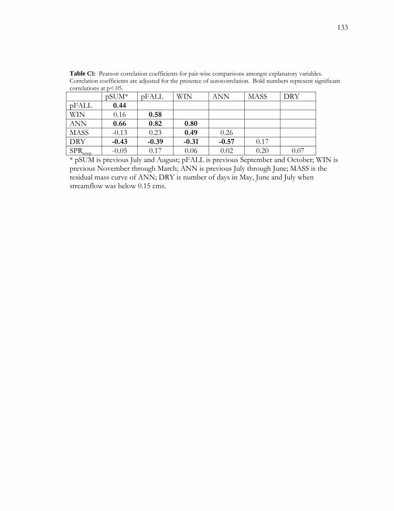
133
Table C1: Pearson correlation coefficients for pair-wise comparisons amongst explanatory variables. Correlation coefficients are adjusted for the presence of autocorrelation. Bold numbers represent significant correlations at p<.05. pSUM* pFALL WIN ANN MASS DRY pFALL 0.44 WIN 0.16 0.58 ANN 0.66 0.82 0.80 MASS -0.13 0.23 0.49 0.26 DRY -0.43 -0.39 0.17 -0.31 -0.57 SPRtemp -0.05 0.17 0.06 0.02 0.20 0.07 * pSUM is previous July and August; pFALL is previous September and October; WIN is previous November through March; ANN is previous July through June; MASS is the residual mass curve of ANN; DRY is number of days in May, June and July when streamflow was below 0.15 cms.
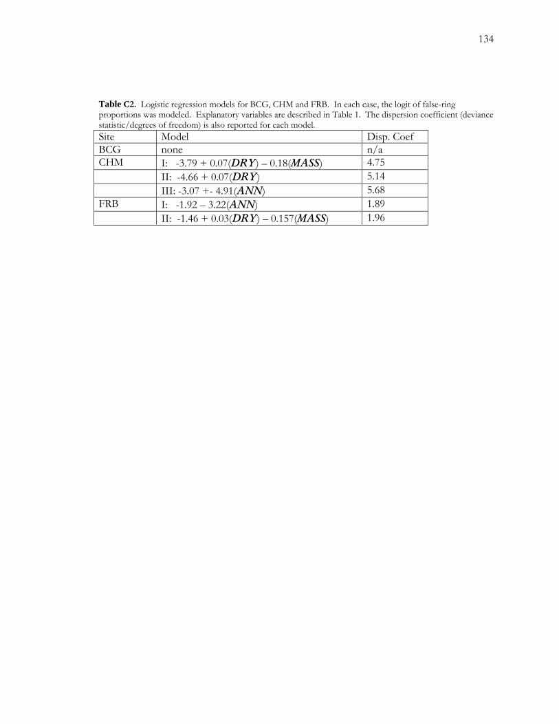
134
Table C2. Logistic regression models for BCG, CHM and FRB. In each case, the logit of false-ring proportions was modeled. Explanatory variables are described in Table 1. The dispersion coefficient (deviance statistic/degrees of freedom) is also reported for each model. Site Model Disp. Coef BCG none n/a CHM I: -3.79 + 0.07(DRY) – 0.18(MASS) 4.75 II: -4.66 + 0.07(DRY) 5.14 5.68 III: -3.07 +- 4.91(ANN) FRB 1.89 I: -1.92 – 3.22(ANN) 1.96 II: -1.46 + 0.03(DRY) – 0.157(MASS)
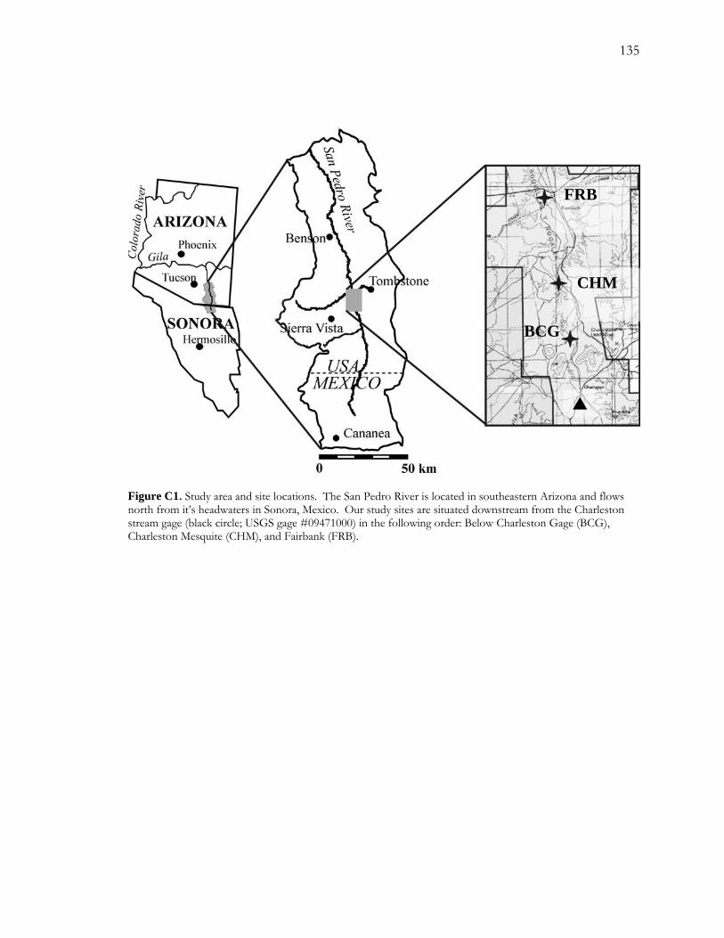
135
FRB
CHM
BCG
Figure C1. Study area and site locations. The San Pedro River is located in southeastern Arizona and flows north from it’s headwaters in Sonora, Mexico. Our study sites are situated downstream from the Charleston stream gage (black circle; USGS gage #09471000) in the following order: Below Charleston Gage (BCG), Charleston Mesquite (CHM), and Fairbank (FRB).
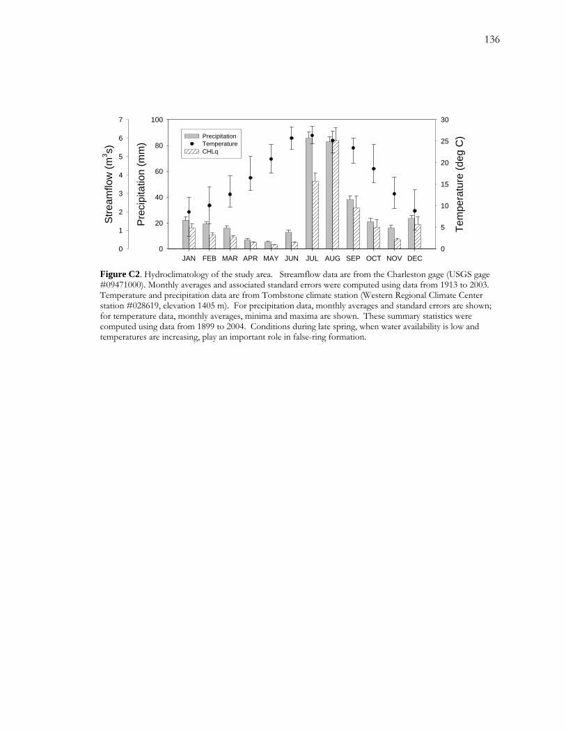
136
JAN FEB MAR APR MAY JUN JUL AUG SEP OCT NOV DEC
Pre
cipi
tatio
n (m
m)
0
20
40
60
80
100
Tem
pera
ture
(deg
C)
0
5
10
15
20
25
30S
tream
flow
(m3 s)
0
1
2
3
4
5
6
7
PrecipitationTemperatureCHLq
Figure C2. Hydroclimatology of the study area. Streamflow data are from the Charleston gage (USGS gage #09471000). Monthly averages and associated standard errors were computed using data from 1913 to 2003. Temperature and precipitation data are from Tombstone climate station (Western Regional Climate Center station #028619, elevation 1405 m). For precipitation data, monthly averages and standard errors are shown; for temperature data, monthly averages, minima and maxima are shown. These summary statistics were computed using data from 1899 to 2004. Conditions during late spring, when water availability is low and temperatures are increasing, play an important role in false-ring formation.
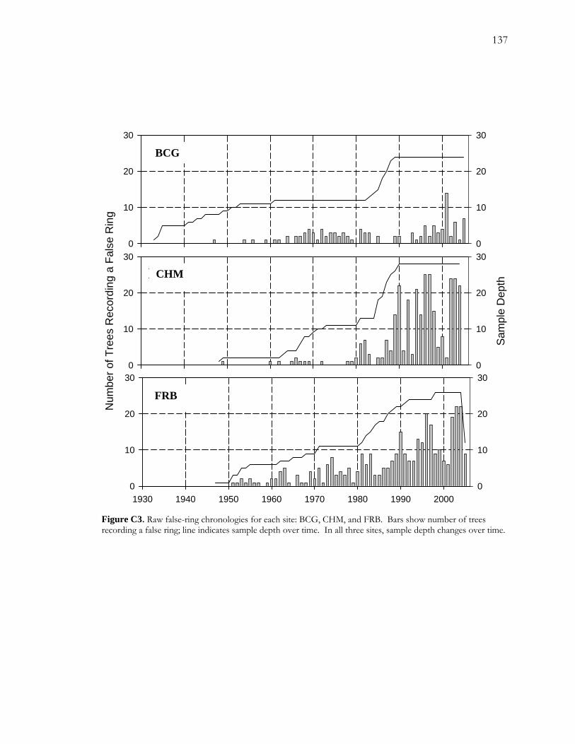
137
0
10
20
30
0
10
20
30
Num
ber o
f Tre
es R
ecor
ding
a F
alse
Rin
g
0
10
20
30
Sam
ple
Dep
th
0
10
20
30
1930 1940 1950 1960 1970 1980 1990 20000
10
20
30
0
10
20
30
A.
C.
B.
BCG
CHM
FRB
Figure C3. Raw false-ring chronologies for each site: BCG, CHM, and FRB. Bars show number of trees recording a false ring; line indicates sample depth over time. In all three sites, sample depth changes over time.
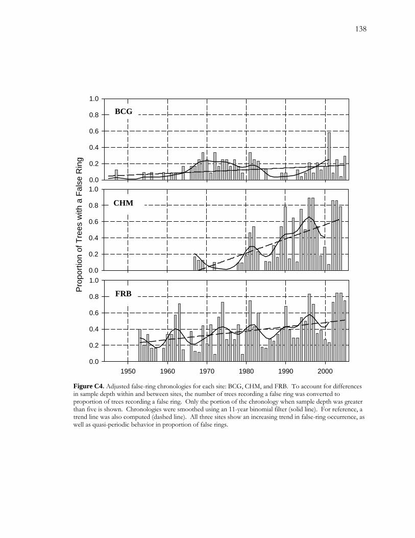
138
0.0
0.2
0.4
0.6
0.8
1.0
0.0
0.2
0.4
0.6
0.8
1.0
1950 1960 1970 1980 1990 2000
Prop
ortio
n of
Tre
es w
ith a
Fal
se R
ing
0.0
0.2
0.4
0.6
0.8
1.0
BCG
CHM
FRB
Figure C4. Adjusted false-ring chronologies for each site: BCG, CHM, and FRB. To account for differences in sample depth within and between sites, the number of trees recording a false ring was converted to proportion of trees recording a false ring. Only the portion of the chronology when sample depth was greater than five is shown. Chronologies were smoothed using an 11-year binomial filter (solid line). For reference, a trend line was also computed (dashed line). All three sites show an increasing trend in false-ring occurrence, as well as quasi-periodic behavior in proportion of false rings.
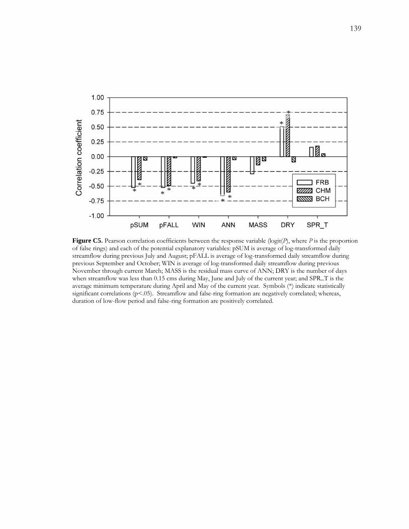
139
**
** **** **
Figure C5. Pearson correlation coefficients between the response variable (logit(P), where P is the proportion of false rings) and each of the potential explanatory variables: pSUM is average of log-transformed daily streamflow during previous July and August; pFALL is average of log-transformed daily streamflow during previous September and October; WIN is average of log-transformed daily streamflow during previous November through current March; MASS is the residual mass curve of ANN; DRY is the number of days when streamflow was less than 0.15 cms during May, June and July of the current year; and SPR_T is the average minimum temperature during April and May of the current year. Symbols (*) indicate statistically significant correlations (p<.05). Streamflow and false-ring formation are negatively correlated; whereas, duration of low-flow period and false-ring formation are positively correlated.
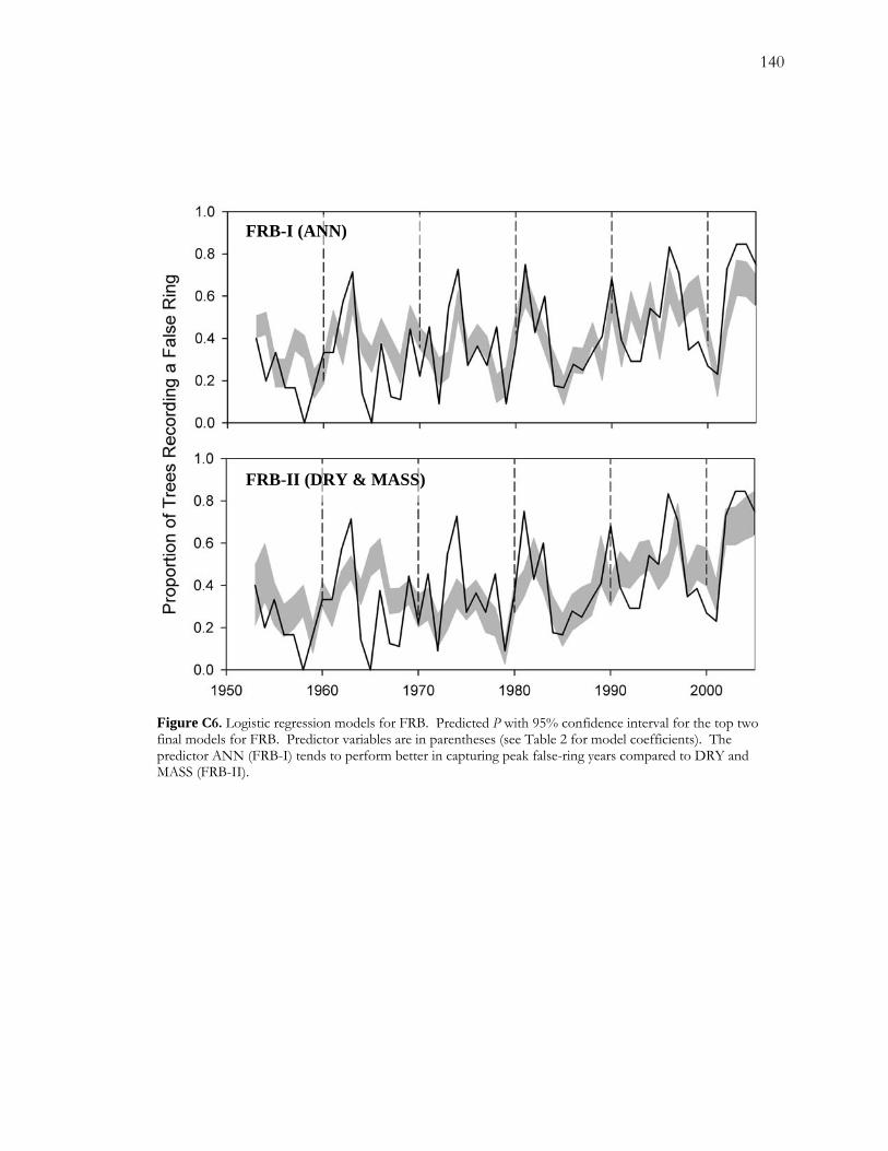
140
FRB-I (ANN)
FRB-II (DRY & MASS)
Figure C6. Logistic regression models for FRB. Predicted P with 95% confidence interval for the top two final models for FRB. Predictor variables are in parentheses (see Table 2 for model coefficients). The predictor ANN (FRB-I) tends to perform better in capturing peak false-ring years compared to DRY and MASS (FRB-II).
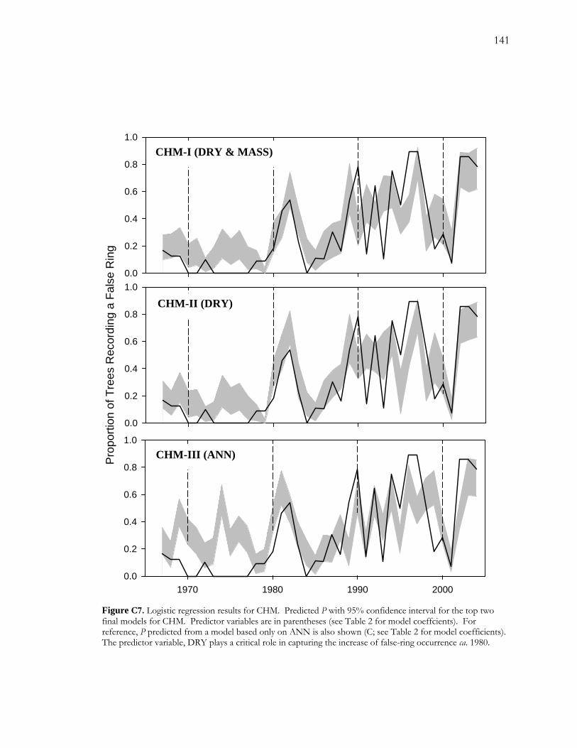
141
1970 1980 1990 20000.0
0.2
0.4
0.6
0.8
1.0
0.0
0.2
0.4
0.6
0.8
1.0
Pro
porti
on o
f Tre
es R
ecor
ding
a F
alse
Rin
g
0.0
0.2
0.4
0.6
0.8
1.0
CHM-I (DRY & MASS)
CHM-II (DRY)
CHM-III (ANN)
Figure C7. Logistic regression results for CHM. Predicted P with 95% confidence interval for the top two final models for CHM. Predictor variables are in parentheses (see Table 2 for model coeffcients). For reference, P predicted from a model based only on ANN is also shown (C; see Table 2 for model coefficients). The predictor variable, DRY plays a critical role in capturing the increase of false-ring occurrence ca. 1980.
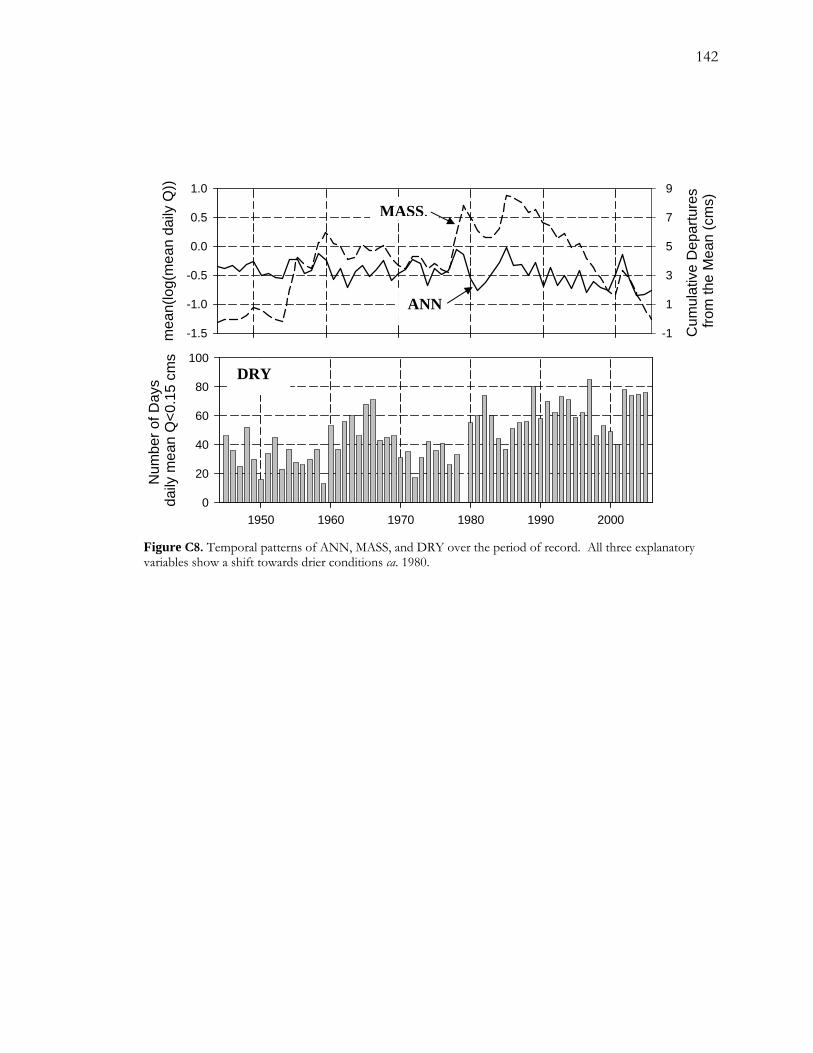
142
-1.5
-1.0
-0.5
0.0
0.5
1.0
-1
1
3
5
7
9m
ean(
log(
mea
n da
ily Q
))
Cum
ulat
ive
Dep
artu
res
from
the
Mea
n (c
ms)MASS.
ANN
0
20
40
60
80
100
Num
ber o
f Day
s da
ily m
ean
Q<0
.15
cms
DRY
1950 1960 1970 1980 1990 2000
Figure C8. Temporal patterns of ANN, MASS, and DRY over the period of record. All three explanatory variables show a shift towards drier conditions ca. 1980.
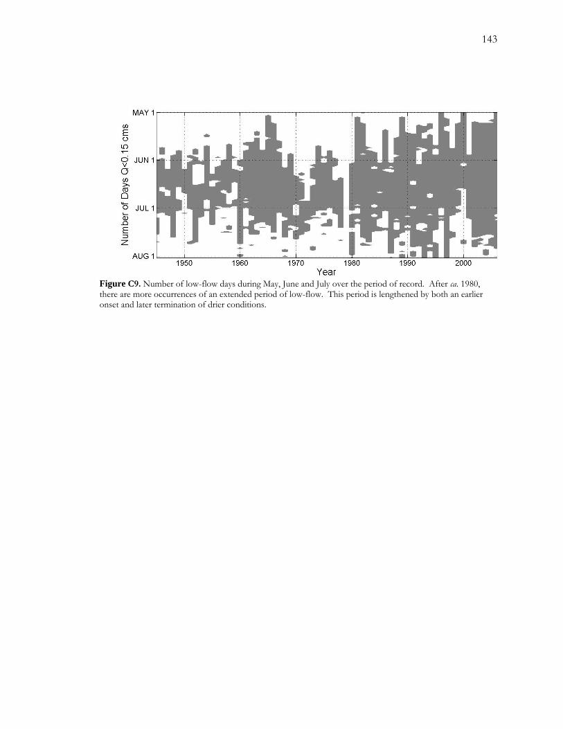
143
Figure C9. Number of low-flow days during May, June and July over the period of record. After ca. 1980, there are more occurrences of an extended period of low-flow. This period is lengthened by both an earlier onset and later termination of drier conditions.
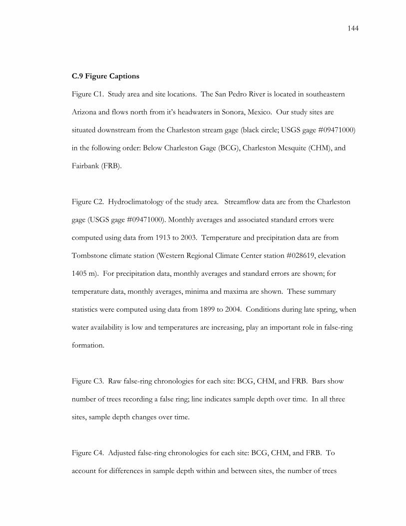
144
C.9 Figure Captions
Figure C1. Study area and site locations. The San Pedro River is located in southeastern
Arizona and flows north from it’s headwaters in Sonora, Mexico. Our study sites are
situated downstream from the Charleston stream gage (black circle; USGS gage #09471000)
in the following order: Below Charleston Gage (BCG), Charleston Mesquite (CHM), and
Fairbank (FRB).
Figure C2. Hydroclimatology of the study area. Streamflow data are from the Charleston
gage (USGS gage #09471000). Monthly averages and associated standard errors were
computed using data from 1913 to 2003. Temperature and precipitation data are from
Tombstone climate station (Western Regional Climate Center station #028619, elevation
1405 m). For precipitation data, monthly averages and standard errors are shown; for
temperature data, monthly averages, minima and maxima are shown. These summary
statistics were computed using data from 1899 to 2004. Conditions during late spring, when
water availability is low and temperatures are increasing, play an important role in false-ring
formation.
Figure C3. Raw false-ring chronologies for each site: BCG, CHM, and FRB. Bars show
number of trees recording a false ring; line indicates sample depth over time. In all three
sites, sample depth changes over time.
Figure C4. Adjusted false-ring chronologies for each site: BCG, CHM, and FRB. To
account for differences in sample depth within and between sites, the number of trees
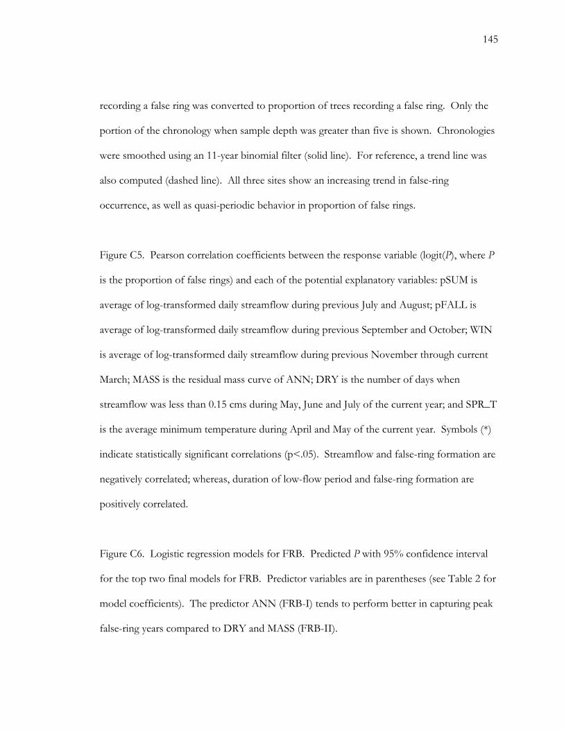
145
recording a false ring was converted to proportion of trees recording a false ring. Only the
portion of the chronology when sample depth was greater than five is shown. Chronologies
were smoothed using an 11-year binomial filter (solid line). For reference, a trend line was
also computed (dashed line). All three sites show an increasing trend in false-ring
occurrence, as well as quasi-periodic behavior in proportion of false rings.
Figure C5. Pearson correlation coefficients between the response variable (logit(P), where P
is the proportion of false rings) and each of the potential explanatory variables: pSUM is
average of log-transformed daily streamflow during previous July and August; pFALL is
average of log-transformed daily streamflow during previous September and October; WIN
is average of log-transformed daily streamflow during previous November through current
March; MASS is the residual mass curve of ANN; DRY is the number of days when
streamflow was less than 0.15 cms during May, June and July of the current year; and SPR_T
is the average minimum temperature during April and May of the current year. Symbols (*)
indicate statistically significant correlations (p<.05). Streamflow and false-ring formation are
negatively correlated; whereas, duration of low-flow period and false-ring formation are
positively correlated.
Figure C6. Logistic regression models for FRB. Predicted P with 95% confidence interval
for the top two final models for FRB. Predictor variables are in parentheses (see Table 2 for
model coefficients). The predictor ANN (FRB-I) tends to perform better in capturing peak
false-ring years compared to DRY and MASS (FRB-II).
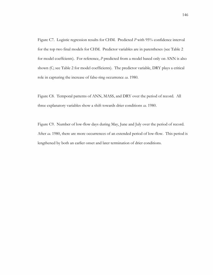
146
Figure C7. Logistic regression results for CHM. Predicted P with 95% confidence interval
for the top two final models for CHM. Predictor variables are in parentheses (see Table 2
for model coeffcients). For reference, P predicted from a model based only on ANN is also
shown (C; see Table 2 for model coefficients). The predictor variable, DRY plays a critical
role in capturing the increase of false-ring occurrence ca. 1980.
Figure C8. Temporal patterns of ANN, MASS, and DRY over the period of record. All
three explanatory variables show a shift towards drier conditions ca. 1980.
Figure C9. Number of low-flow days during May, June and July over the period of record.
After ca. 1980, there are more occurrences of an extended period of low-flow. This period is
lengthened by both an earlier onset and later termination of drier conditions.