Using IRT DIF Methods to Evaluate the Validity of Score Gains

CSE Technical Report 660

Daniel M. Koretz

CRESST/Harvard Graduate School of Education

Daniel F. McCaffrey RAND

September 2005

National Center for Research on Evaluation, Standards, and Student Testing (CRESST) Center for the Study of Evaluation (CSE)

Graduate School of Education & Information Studies University of California, Los Angeles

GSE&IS Bldg., Box 951522 Los Angeles, CA 90095-1522

(310) 206-1532

Project 1.1 Comparative Analyses of Current Assessment and Accountability Systems; Strand 3: The Validation of Gains Daniel Koretz, Project Director, CRESST/Harvard Graduate School of Education Copyright © 2005 The Regents of the University of California The work reported herein was supported under the Educational Research and Development Centers Program, PR/Award Number R305B960002, as administered by the Institute of Education Sciences, U.S. Department of Education. The findings and opinions expressed in this report do not reflect the positions or policies of the National Center for Education Research, the Institute of Education Sciences, or the U.S. Department of Education.

USING IRT DIF METHODS TO EVALUATE

THE VALIDITY OF SCORE GAINS

Daniel M. Koretz, CRESST/Harvard Graduate School of Education

Daniel F. McCaffrey, CRESST/RAND

Abstract

Given current high-stakes uses of tests, one of the most pressing and difficult problems confronting the field of measurement is to develop better methods for distinguishing between meaningful gains in performance and score inflation. This study explores the potential usefulness of adapting differential item functioning (DIF) techniques for this purpose. We distinguish between reactive and nonreactive changes in DIF over time and relate these to the framework for validating scores under high-stakes conditions offered by Koretz, McCaffrey, and Hamilton (2001). We contrast score-anchored and item-anchored approaches to DIF in terms of their potential for this purpose. We explored changes in the distribution of DIF in the NAEP eighth-grade mathematics assessment between 1990 and 2000 in five low-gain and five high-gain states, in each case treating all other participating states as the reference group. We used the score-anchored method of DIF analysis implemented in BILOG-MG (Bock & Zimowski, 2003b), which allows only item difficulties to vary across groups. This exploration indicated that the approach has potential but confronts several substantial difficulties. Further exploration using data from high-stakes testing programs is recommended.

One of the most pressing and difficult problems confronting the field of measurement today is to develop more powerful methods for distinguishing meaningful cohort-to-cohort gains in performance from score inflation. Score inflation is defined here simply as increases in scores not accompanied by commensurate increases in the aspects of achievement about which score-based inferences are drawn. Studies of a number of high-stakes testing programs have shown that the inflation can be very large when educators are held accountable for scores. In some cases, observed gains on high-stakes tests have been several times as large as gains on other measures, while in other cases, gains on high-stakes tests have been accompanied by no improvement whatever on other measures (e.g., Jacob, 2002; Klein, Hamilton, McCaffrey, & Stecher, 2000; Koretz & Barron, 1998; Koretz, Linn, Dunbar, & Shepard, 1991). The current pervasiveness of high-stakes uses of tests raises the prospect of widespread score inflation that could mislead policymakers and the public about the condition of education. Moreover, to the

1

extent that score inflation is non-uniform, inferences about the relative effectiveness of schools and the impact of educational interventions may be fundamentally incorrect. The result may be inappropriate application of rewards and sanctions and a misdirection of innovation.

Most empirical studies of the validity of gains in scores on high-stakes (or focal) tests have examined the degree to which these gains generalize to other (audit) measures, such as the National Assessment of Educational Progress (NAEP), that have not been the explicit focus of test preparation (e.g., Klein et al., 2000; Koretz & Barron, 1998; Koretz et al., 1991). However, this approach is informative only when there is a very large disparity in trends on the two tests (Koretz, 2002). The degree to which generalizability is to be expected depends on the specific inferences users base on scores and the consistency of both measures with those inferences. Because systematic information about these considerations is rarely available, modest differences in trends are difficult to interpret.

Accordingly, Koretz, McCaffrey, and Hamilton (2001) argued that to evaluate the validity of gains in scores on high-stakes tests more precisely, one would need to identify the specific sources of gains in scores and compare these to the inferences based on score gains. The validity of an inference about gains then depends on the degree of concordance between the specific patterns of gains shown by the elements included in the test and the patterns of gains assumed by the inference. Applying this framework requires identifying the elements that make large contributions to gains in scores.

This study explores the potential utility of differential item functioning (DIF) methods for identifying the sources of score gains between cohorts of students from the same educational unit (state, school district, or school). Specifically, we explore one class of IRT-based DIF methods. The methods are tested using state-level NAEP data in eighth grade mathematics from 1990 through 2000. The report discusses within- and between-state distributions of DIF, but the arguments would pertain to any unit of analysis within which score inflation might occur and sufficient data exist for conducting the analyses.

The report is divided into several sections. The first sections reconceptualize score inflation in terms of DIF, introduce the concepts of reactive and non-reactive DIF, and link these to the IRT methods chosen for this study. The middle sections

2

describe some technical details of the methods used in this study and present the principal findings. The final section discusses implications for future research.

A Model of Validity Under High-Stakes Conditions

Koretz, McCaffrey, and Hamilton (2001) consider the inferences that can be derived from aggregate cohort-to-cohort gains over time in standardized test scores. They conceptualize the validity of inferences about gains under high-stakes conditions (VIHS) in terms of performance elements. This term refers to all of the aspects of performance that underlie both performance on a test and inferences based on it. Some of these performance elements are substantive and contribute either explicitly or tacitly to the definition of the construct or domain about which inferences are drawn. Others are nonsubstantive. For example, the use of particular item formats may be nonsubstantive and therefore can introduce construct-irrelevant variability in performance.

Although evaluation of tests traditionally focuses on the cross-sectional correlations among items, VIHS depends also on the potential for performance on elements to vary independently over time. As Koretz et al. (2001) point out, performance elements that are correlated in cross-section may nonetheless change independently over time. For example, in a typical secondary-school mathematics test, performance in algebra and geometry will typically be highly collinear. Nonetheless, if schools increased instruction in algebra by requiring it for all students but made no changes to instruction in geometry, performance in algebra would be expected to change independently of performance in geometry over time. A concrete example of the importance of this fact is found in a study of score gains in Kentucky by Koretz and Barron (1998). The authors compared school-level performance on the ACT and the state’s high school accountability test. Over a period of 3 years, means on the two tests among students who took both diverged by roughly 0.7 standard deviation, but the school- and student-level correlations between mathematics scores on the state test and the ACT remained stable.

Both a test and inferences based on scores assign weights—that is, varying degrees of importance to the various performance elements they comprise. Koretz et al. (2001) defined the “effective test weight” of a performance element as the sensitivity of the test score to changes in performance on that element. Specifically, where the score θ is any function of the vector of performance elements , π

3

(1) ( )fθ = π

the effective weight of element iw iπ is:

(2) ii

w θπ∂

=∂

.

They note that these weights can depend on many factors, some of which can be unintended by test developers and are therefore not necessarily the same as suggested by test specifications. Similarly, users of tests assign “inference weights” to performance elements in drawing inferences about student achievement, although these weights are usually poorly formed and partially tacit. The composite of elements with substantial inference weights was labeled the “target of inference” by Koretz et al. (2001). Because the items included on tests are usually very limited samples from large domains, elements that are important for an inference may be given little or even no weight in a test. Such elements are called “implicit” performance elements by Koretz et al. (2001).

From this perspective, the validity of gains can be seen in terms of the concordance between changes on tested elements and changes on elements with large inference weights. Increases in scores will stem from changes in performance on certain elements—in particular, those with particularly large gains, particularly large weights, or both. Users will draw inferences about a partially overlapping set of elements, necessarily if implicitly assigning weights to them. Inflation occurs when increases in performance on the elements emphasized by the test become unrepresentative of the domain in the sense that they do not warrant inferences about commensurate changes in the set of elements with large inference weights. The latter set is likely to include some implicit elements.

Inflation can then arise from either of two general mechanisms. One mechanism is biases in the estimates of individual iπ -- that is, overestimates of the increase in performance on specific elements. A wide variety of responses to high stakes can cause these biases (see Koretz et al., 2001, for a taxonomy of methods of test preparation). For example, it can arise from simple cheating or from instruction that emphasizes test-taking tricks. In addition, it can arise from the responses that Koretz et al. (2001) label “coaching,” of which they distinguish two types:

Substantive coaching refers to an instructional emphasis on narrow aspects of substantive performance elements to comport with the style or emphasis of test items….Non-

substantive coaching refers to forms of test preparation that focus instruction on elements

4

of the test that are largely or entirely unrelated to the definition of the domain the test is intended to represent. (Koretz, McCaffrey, & Hamilton, 2001, pp. 20-21)

The second mechanism by which scores become inflated need not entail any bias in estimates of individual iπ but generates bias when the iπ are aggregated into

scores. One such process was labeled “reallocation” by Koretz et al. (2001). Educators can reallocate instructional resources from elements with low test weights to elements with larger test weights. If the deemphasized elements have substantial inference weights, this reallocation creates inflation when the performance elements are aggregated into a test score. It is for this reason that implicit elements are potentially much more problematic for the validity of VIHS than for the validity of cross-sectional score-based inferences under lower stakes conditions. High stakes can create incentives to deemphasize material not emphasized by the test.

Thus, score inflation can be seen as an issue of the dimensionality of changes in scores. Scores become inflated when increases in performance along dimensions well measured by the test do not imply commensurate increases along dimensions less well measured but still important for inferences. Because changes in performance dimensions can be uncorrelated even when cross-sectional correlations among them are high, change scores can be multidimensional even if the test is effectively unidimensional according to conventional tests of dimensionality. Conventional tests of the dimensionality of scores (e.g., scree tests) are cross-sectional. They do not evaluate the degree to which changes in performance are multidimensional and therefore cannot rule out inflation. To identify score inflation we need to develop methods for identifying multidimensionality in changes in scores. Differential Item Functioning (DIF) may provide such a method.

Differential Item Functioning

DIF analysis is one way of exploring dimensionality in cross-sectional data, and this report explores the usefulness of extending it to the analysis of change under high-stakes conditions. DIF refers to group differences in the statistical functioning of an item among individuals who have been matched on an index of the proficiency the test is intended to measure. DIF is most often used to explore possible item bias. For that purpose, comparisons are made between a subgroup that is a focus of concern, called the focal group, and a subgroup for whom the test is assumed to be acceptable, called the reference group. Items that show sufficient DIF are typically candidates for deletion. However, cross-sectional DIF analysis can be applied to a

5

much wider range of problems. DIF analysis can be applied to group differences without assumptions about the adequacy of measurement in reference groups, and can be used to create between-group adjustments in scores rather than as a basis for screening items for deletion. For example, King, Murray, Salomon, and Tandon (2004) used DIF methods to generate adjustment factors to increase the cross-national comparability of responses to survey questions about disabilities.

The existence of DIF need not imply item bias, but it does indicate that the test at issue is multidimensional. If a test were truly unidimensional, a single overall proficiency scale would account for all systematic variations in performance, and one would find only random differences within groups matched in terms of proficiency. Of course, no broad test of achievement is truly unidimensional; the question for most purposes is the degree to which a test violates this assumption. Cross-sectional DIF analysis evaluates the extent of one type of possible deviation from cross-sectional unidimensionality. DIF arises when there is at least one dimension of proficiency other than the primary dimension measured by the test that is distributed differently in two groups and causes individuals in those groups with similar proficiency to perform differentially on specific items.

The study reported here represents an effort to extend the logic and method of DIF to the evaluation of score inflation. It is an exploration of the extent to which a specific type of multidimensional model is needed to address changes in performance under high-stakes conditions. This extension is not straightforward. Because score inflation is only one of many sources that could produce a change in DIF over time, it is necessary to compare changes in DIF in at least two settings that differ in the propensity for the behavioral changes that can cause inflation. This is described below.

Over the past several decades, a wide variety of methods have been devised for exploring DIF (see, for example, Camilli & Shepard, 1994; Holland & Wainer, 1993). The most common approaches are the Mantel-Haenszel chi-square, logistic-regression methods, and methods based on IRT models. A substantial literature compares these approaches (e.g., Angoff, 1993; Zwick, 1990), but for our purposes, the differences among them are not of primary importance, as they are conceptually and in some instances mathematically similar. We have chosen to use IRT-based methods for several reasons, including the convenience of the theta metric, the ability over the longer term to examine DIF affecting item discrimination as well as

6

item difficulty, and the ability to perform item-anchored as well as score-anchored analyses, as described below.

Score-Anchored and Item-Anchored Approaches to DIF

More important for our purposes is the conceptual difference between what we call score-anchored and item-anchored approaches to DIF. Score-anchored analyses use some variant of the test score as the criterion for matching individuals across groups—for example, a total number-right score, a score obtained by deleting the particular item under investigation, or a theta estimate based on the entire test. The large majority of DIF analyses in the measurement literature are score-anchored, and many discussions of DIF take this as a given and do not address item-anchored approaches. The assumption underlying score-anchored approaches is that the particular score used as the matching criterion has the same meaning across the groups being compared. Many observers (e.g., Angoff, 1993) have pointed out that there is an inherent logical inconsistency in the score-anchored approach. At different points in the analysis, any given item is used both as the target of DIF analysis and as part of the matching criterion for testing for DIF in other items. Items are treated as acceptable when they are used for matching but as questionable when they are the focus of investigation.

The alternative approach we call item-anchored. In this approach, certain items are selected on some basis to be DIF-free, that is, to function similarly across groups. The basis for this selection could be design, theory, empirical data, or a combination of the three. Rather than using a total score to match individuals, these DIF-free items are used as an anchor. The item-anchored approach was used, for example, by King et al. (1994), who designed vignettes specifically to be free of cross-national differences in response patterns and adjusted responses to survey items based on responses to these vignettes, using a Rasch DIF approach.

Although the score- and item-anchored DIF approaches differ in concept, they actually anchor two ends of a continuum, and many DIF analyses fall in between. In response to the logical inconsistency inherent in the score-anchored approach, some investigators use an iterative score-anchored approach in which items that exhibit DIF are gradually eliminated from the score used for matching. This results in a “purified” matching criterion. One could see this iterative process as a modification of the score-anchored approach, but one could also see it as an entirely ad hoc, empirical procedure for identifying the items to be used in an item-anchored

7

approach. In practice, this purification procedure usually bears more resemblance to the score-anchored approach. The percentage of items eliminated is often small, leaving the majority of items in the purified matching criterion. In contrast, the item-anchored approach can be carried out with only a small number of items used as anchors. For example, Wang and Yeh (2003) found in a simulation study that increasing the number of anchor items from 4 to 10 provided only modest reductions in the frequency of Type I error and very small increases in power. Moreover, the purified-DIF approach employs typically estimation methods used with score-based methods, whereas purely item-anchored analyses often employ different estimation methods, as explained below.

The distinction between score- and item-anchored approaches was placed in an IRT context by Thissen, Steinberg, and Wainer (1993), albeit with a different terminology. Thissen et al. (1993) labeled as “IRT-D2” a score-anchored IRT method that is implemented in the DIF and DRIFT procedures in BIMAIN and BILOG (see also Bock and Zimowski, 2003a, 2003b). In this approach, two calibration runs are compared: one that pools the two groups in question into a single group, and a second calibration that treats the two groups as distinct. In the latter, the asymptotes and guessing parameters are held constant across groups, but the difficulty parameters are allowed to differ between them. However, the intent is to test only for interactions between item and group. Therefore, the group means of the item difficulty estimates are set to be equal. This is done by subtracting the mean difference in difficulties between the focal and reference group from the difficulty estimates for each item in the focal group. Thus, where f and r index the focal and reference groups, DIF for item i is:

(3) ( )ˆ ˆ ˆ ˆif if if ir f rDIF b b b bδ= = − − − .

The statistical significance of DIF across all items is tested by comparing the two calibrations using the standard likelihood ratio test.

It may not be immediately apparent why this procedure, which places a constraint on item parameters, is a score-anchored method. In any IRT model, b and

θ are on the same scale. In the calibration in which the b parameters are free to vary across groups, these scales are not initially the same in the two groups. (Indeed, they will be different by construction if the two groups differ in mean proficiency because the scaling procedure will set either the mean of bi or the mean of θ to zero in both groups.) Setting the mean bi to be equal is one means of linking the initially

8

arbitrary scales across the two groups; it places θ on the same scale in both groups but leaves the distribution of θ free to vary between the groups. The result is to treat differences in the theta distribution as meaningful differences in proficiency (Bock & Zimowski, 2003a, 2003b). That is, because the difficulty estimate for the average item is constrained to be constant between the groups, any difference in performance between groups on the average item must represent differences in proficiency. But now suppose that one item generates a different b in the two groups, even after the means of the bi estimates are adjusted to be equal. That means that the item is harder for individuals in one group than for individuals in the other group who have the same θ . Thus, individuals across groups have been matched on θ , and this anchor reflects all items, regardless of whether they demonstrate DIF.

Thissen et al. (1993) contrasted this with an item-anchored approach that they termed “general IRT-LR.” In this approach, some items are selected (by whatever criterion) to be treated as free of DIF. The two groups are calibrated together, holding the parameters of the DIF-free anchor items fixed and allowing the parameters of the other items to differ across the two groups (see also Thissen, 2003). This approach is readily generalized to tests of all three parameters in a 3-PL model.

The two approaches differ fundamentally in the assumptions they make in anchoring the scales in the two groups. The IRT-D2 method allows any item to display DIF and incorporates it into the matching criterion regardless by of holding constant across groups the mean difficulty of all items. It is thus is consistent with all DIF methods that condition on a total-score measure. Like all such score-anchored methods, it suffers from the logical inconsistency noted by Angoff (1993) and others. Moreover, this logical inconsistency has a practical consequence: if DIF is actually primarily in one direction, score-anchored methods will attenuate the magnitude of this DIF and generate spurious DIF in the opposite direction. This is a consequence of the fact that the interactions tested by the model sum to zero. For example, suppose true DIF, if accurately measured, favored the reference group on 10% of items on a given test and that all other items are in (unmeasured) fact DIF-free. The DIF showed by the 10% of items would depress the mean score of the focal group. Because the performance of focal group members would be conditioned on this downwardly biased mean, the estimated magnitude of DIF on the 10% would be attenuated, and other items with no true DIF would necessarily show spurious DIF favoring the focal group. Moreover, as explained below, score-anchored methods are not ideal for examining DIF caused by score inflation.

9

In contrast, item-anchored DIF approaches such as the general IRT-LR method require no assumption about mean differences in performance. They avoid the logical inconsistency inherent in score-anchored approaches, and for the same reason, they avoid the empirical problems that this inconsistency entails. In addition, if they were practical, they would circumvent the specific weaknesses of score-anchored methods for the investigation of score inflation. However, they do require either an assumption or empirical evidence that differences in performance on the specific items chosen as anchors are meaningful and are not a result of construct-irrelevant DIF. In many cases, there is no basis for such an assumption.

DIF and Score Inflation

This framework for describing validity under high-stakes conditions (VUHSC) and score inflation can be re-expressed readily in terms of DIF. Score inflation may occur when increases in performance are differential across the performance elements with substantial inference weights. More precisely, while not all increases that are differential across these elements will cause score inflation, all score inflation entails differential increases. These differential gains will create multidimensionality, which will appear as DIF if they are non-uniform across identifiable groups that can be compared. Consider both the mechanisms of score inflation noted earlier, and for this example ignore the spurious offsetting DIF that score-anchored methods create. If a group—say, a school or a state—inflates scores by means of activities that inflate estimates of an element 1π , the result will be positive DIF affecting items measuring 1π but no DIF affecting other items. If that same group creates inflation by reallocation, this would show up as positive DIF affecting items measuring any 1π that receives additional emphasis and negative DIF affecting items measuring any 1π that it deemphasized. Thus if we have two or more groups that might differ in their responses to testing, DIF analyses might be used to identify potential score inflation.

The difficulty in treating score inflation as DIF is a variant of a problem that affects most DIF analysis: the lack of an unambiguous basis for matching individuals to identify differential performance. If score inflation affects some elements and items more than others, we expect students in groups with and without inflation who are matched on “true” proficiency to perform differentially across performance elements and different items. “True” performance here refers to performance as measured by an instrument unaffected by inflation. Such an instrument would have

10

to include the elements relevant to the inference, assign them effective test weights consistent with inference weights, and be free of the biases in estimates of individual elements caused by coaching or cheating. Even though the measure could not be exhaustive, it would need to include implicit elements given large inference weights, if those elements were at risk of de-emphasis because of test preparation. Clearly, such an ideal matching criterion will not be available. The way in which students are matched using a proxy for this unavailable measure will determine our estimates of DIF.

Indeed, in most cases, there will be no external matching criterion available, and the analyst will have to make do with internal measures constructed from the test being analyzed. There are two primary alternatives for constructing an internal matching criterion. The first is score anchoring: matching individuals on some measure of overall performance on the test, generally using the effective weights in the operational test. The second is item anchoring: matching individuals on their performance on specific items chosen to be free of possible distortions from test preparation. In the context of periodic testing over time with partially new forms, two groups of items are obvious candidates for item-anchored DIF analysis: reused items that appeared in previous administrations and new items that are used for the first time on the test under study.

Matching on some function of total scores has the advantage of not requiring any assumptions about individual test items. Moreover, procedures for score-anchored DIF analysis are numerous and well known. However, score anchoring also has several important disadvantages. One, noted above, is that the matching criterion is contaminated by the DIF one is attempting to measure. As in many DIF analyses, there is the possibility that much or all of the test is biased for some reason and that score anchored methods therefore fail to show DIF. In the context of potential score inflation, this might occur if inflation were caused by reallocation away from implicit performance elements with sizable inference weights but low test weights. Another problem with this method is that because DIF must average zero, any substantive DIF in either direction must necessarily be offset by apparent DIF in the other direction on other items. Therefore, the absolute value of the DIF statistic for a given item is not directly interpretable, and one can only identify relative differences in performance.

If one could identify items free of inflation to serve as anchors, one might ameliorate these problems but not necessarily eliminate them. For example,

11

suppose one could identify items on which performance is free of distortion from coaching or cheating. Performance on these items would nonetheless be flawed as a matching criterion to the extent that inflation stems from reallocation away from elements with large inference weights that are not included in the test (and therefore not in the item anchor set). Moreover, it is not clear how feasible it will be to identify even items that are free of the effects of coaching and cheating.

A common approach to linking scales over time uses as anchors items that are kept secure and reused over time. One might similarly use these items as anchors in an item-anchored DIF approach. However, this does not seem tenable because the necessary assumption that the true difficulty of a linking item is constant is not warranted. (More precisely, the necessary assumption is that the relationship between the difficulty of these items and the latent proficiency is constant.) To the extent that the content and style of secure items is remembered, they can serve as the basis of inappropriate test preparation despite test security, and this will change the relationship between item difficulty and the latent proficiency. Koretz and Barron (1998) showed evidence suggestive of coaching on reused items and argued that this process, when used to link over time, would build score inflation into the scale. By the same token, coaching on reused items could obscure inflation-based DIF. Anchoring on reused items also is potentially problematic because the reused items cannot cover the entire range of performance elements with significant inference weights. Differences in performance on elements included in the test and in the inference space but excluded from the anchor items could appear as DIF. This DIF identifies multidimensionality but not necessarily score inflation.

Conversely, one might argue that new items should be free of any biases stemming from test preparation and that these could be used as anchors. However, this assumption may also prove untenable. Most tests show strong similarities in both content and style over time. In part, this is intentional when tests must be linked over time, but it may also be unintended. Therefore, the effects of inappropriate test preparation focused on reused items may generalize to varying degrees to new items, and therefore using new items as anchors might lead to an underestimate of inflation-related DIF.

Thus, in this application as in others, findings of DIF are relative to the matching criterion. Moreover, as explained below, changes in DIF stemming from score inflation may be confounded changes in DIF that result from other changes in the educational system, for example curriculum changes. What DIF will identify is

12

differential performance that can identify dimensions in the test. These will require additional investigation to be attributed to score inflation.

Because of the inherent limitations of score-anchored DIF methods, we expect that in the long run, item-anchored methods may be more useful in evaluating the validity of gains. Using this approach may require modifications to the design of testing programs to provide items specifically designed for anchoring, such as items that have high weights but that are by design different from earlier items in terms of irrelevant aspects of content, format, and style. However, at present, given both the lack of empirical information about the mechanics of score inflation and the items designed to be anchors, it appears that a score-anchored method may be more reasonable for initial explorations. Therefore, in the work reported here, we used the IRT-D2 method.

Reactive vs. Non-Reactive DIF

To use DIF methods to explore possible score inflation, we need to expand on the traditional IRT notion of variations in the estimated difficulty of any given item i,

. In common practice, three sources of variation in b are considered: model

specification (the choice of IRT model, the selection of an estimation method, and decisions about priors in the case of Bayesian methods), simple errors of estimation, and violations of the assumption of unidimensionality. Systematic differences between groups in b , holding constant

ib i

i θ , are a violation of the assumption of

unidimensionality and appear as DIF. Variations in other than those stemming

from DIF are treated as unsystematic error of estimation. ib

For our purposes, however, we have to distinguish between two types of systematic differences among groups: those caused by responses to testing and all others. The key to the validity of score gains is systematic differences stemming from responses to testing.

We use the term non-reactive DIF to refer to differences between groups in item difficulty (holding constant proficiency) that do not stem from reactions to testing. Non-reactive DIF can arise from item bias, curricular differences, or other factors that are not responses to the test in question. In large-scale educational assessments, non-reactive DIF is typically analyzed for gender, racial/ethnic subgroups, and sometimes language proficiency. It is occasionally analyzed for geographic subgroups, such as states or nations (e.g., King et al., 2004; O’Connor, 2000). Such

13

DIF is most often considered a nuisance to be minimized, if necessary by deletion of items. However, it can also provide insight into substantive differences in the performance of subgroups (e.g., Wolfe, 1997).

In contrast, reactive DIF refers to differences in item difficulty that arise specifically as a result of responses to testing. A certain class of items—say, items involving pictorial representations of algebraic equalities and inequalities, as used in recent forms of the Massachusetts assessment—may become easier relative to other

items in group that focus test preparation specifically on this type of item, either through coaching or reallocation. Similarly, reallocation can make other classes of items relatively harder, by means of reduced instructional emphasis.1

Distinguishing between reactive and non-reactive DIF requires only minor elaboration of the IRT-D2 model. Recall that this model explores interactions between group and item and that mean differences in performance between groups are absorbed in the distribution of θ rather than the distribution of b. In a conventional cross-sectional application of IRT-D2, the distribution of the estimated item difficulties in the focal group f are recentered to have the same mean as the item difficulties estimated in the reference group:

(4) ( )* ˆ ˆ ˆ .• •= − −if if f rb b b b

DIF for item i, δ i , is then defined as:

(5) * ˆδ = −i ifb bir

and therefore 1 0δ =∑ iin

, that is, the mean DIF over items is by construction zero.

Note that while the sign of the DIF statistic is arbitrary, in this method, the DIF statistic is negative when the item is easier in the focal group. We follow that convention throughout this report.

Rearranging equations 4 and 5, one can express the estimated, unadjusted difficulty of item i in the focal group as the sum of its estimated difficulty in the reference group, the recentering adjustment, and DIF: 1These variations in relative item difficulty are often ignored in scaling and linking, although doing so may seriously bias inferences based on the resulting scale when the test preparation is inappropriate. For example, Koretz and Barron (1998) noted that common IRT equating methods based on the assumption that the true difficulty of items remains constant across forms will build score inflation into the scale when items become easier as a result of inappropriate test preparation.

14

(6) ( )ˆ ˆ ˆ ˆ .δ• •= + − +if ir f r ib b b b

However, δ i can be either reactive or non-reactive and can change over time.

Thus the unadjusted estimated difficulty can be expressed more completely as:

(7) ( )ˆ ˆ ˆ ˆif ir f r if ifb b b b ν γ• •= + − + + ,

where ifν is non-reactive DIF on item i and itγ is reactive DIF. These two sources of

DIF cannot be distinguished with a single year of data. However, we expect that with multiple years of data we might be able distinguish the two sources of DIF because they should behave differently over time. With multiple years of data the model for estimated item difficulty parameters is

(8) ( )ˆ ˆ ˆ ˆ ν γ• •= + − + +ift irt ft rt ift iftb b b b .

When an assessment is new, there has not yet been an opportunity for teachers and students to react to it, so all 1 0ifγ = . Thus, the first year of an assessment can

serve as a baseline, and the distribution of DIF apparent in that year is a combination of non-reactive DIF and estimation error. Reactive DIF will be apparent in changes in DIF over time, as teachers and students have opportunities to respond to the pressures of the test.

DIF may change over time for reasons unrelated to the test. That is, iftν may not

be constant over time, and changes in iftν would then be confounded with reactive

DIF. However, if the test is high stakes, it seems reasonable to assume that changes in DIF over time stem in substantial part from responses to it. Therefore, it appears to be a reasonable simplification to hold non-reactive DIF constant and to assume that changes in DIF over time represent reactive DIF. Moreover, for evaluating the validity of gains, it is not necessarily important to distinguish between reactive DIF and changes in non-reactive DIF. Any local gains on some items that do not generalize to others have the potential to undermine validity. (Here and throughout the report, we use “local” in the psychometric sense of performance specific to part of the test, not to geographically local patterns.)

Expected Patterns of DIF

Given this discussion, one method for potentially identifying score inflation is to use multiple years of data from two or more groups that might have responded differently over time to testing. For example, comparing school districts within a

15

state using multiple years of state tests or comparing different states using the National Assessment of Educational Progress (NAEP). If this approach were followed then what patterns might be expected in the distribution of DIF across items? The distribution of non-reactive DIF at baseline is not predictable. One can estimate the contribution of estimation error to the distribution of DIF, but the contribution of other factors, in particular variations in the curricular alignment of the test, is generally unknown. Therefore, neither the typical within-group, initial distribution of DIF across items nor the variability of these initial distributions across groups can be predicted. Similarly, non-reactive changes in DIF cannot be predicted a priori. For example, consider using NAEP data and states to identify inflation and suppose that the NAEP were to add a content area that had previously not been tested. Major changes of this sort have been made to mathematics assessments a number of times over the past several decades, for example the addition of estimation items and “data analysis and statistics” to many of them. Now suppose that some states had added these content areas to their instruction before the change in the test, while others had not. The result would be an initial increase in the variability of non-reactive DIF across states. Depending on the number of states in each group and the method used to detect DIF, this might show up as DIF favoring one group, disfavoring the other, or both. One can similarly imagine changes in the match between testing and curriculum that would reduce either the amount of non-reactive DIF or its variability across states.

This brings us to the crux of the dilemma alluded to earlier: score-anchored methods are weak tools for investigating the effects of score inflation. One can make only weak predictions about the impact of inflation on the distribution of DIF. Item anchored methods might provide a somewhat stronger tool, but we lack a firm basis for selecting item anchors.

One might expect inflation to increase the within-state variability of DIF, as it adds another source of variance. However, conditions might arise in which the effect could be the reverse. Specifically, variance will increase if the increased emphasis underlying inflation is distributed randomly across items. If teachers focused greater emphasis on items with negative DIF—that is, items on their students show relatively stronger performance, holding proficiency constant—the absolute value of this DIF would increase, and the variance of DIF would increase further. However, if teachers focused greater emphasis on items with positive DIF, those items would become relatively easier, reducing the absolute magnitude of DIF

16

on those items and, absent other changes, reducing the variance of DIF.2 Thus in theory, reactive changes in DIF could appear as a wide variety of changes in the distribution of DIF. In the case of many assessments, however, and particularly in the case of the NAEP, it is hard to see how teachers could discern DIF. To do so would require that they compare the relative performance of their students on a given item to their relative performance on others, taking into account the distortions caused by the percent-correct metric typically used to report item-level results to educators. This seems implausible. Recall also that when using a score-anchored method, the mean of the DIF statistic is always zero by construction, and a real change in DIF in any direction will be both attenuated and accompanied by offsetting changes in the other direction on other items. Therefore, it seems reasonable to expect that reactive DIF would increase the within-state variance of the distribution of the DIF statistic over time.

In contrast, more localized changes in DIF could appear as changes in the skewness of the distribution of the DIF statistic. For example, assume that teachers in a given state focus considerable effort on improving performance on knowledge and skills that are emphasized by a small number of previously used items and that similar items appear in newer forms, also in small number. Assume also that this instruction or coaching is effective but that its effects do not generalize a great deal to other items. The result would be to make these items relatively easier, making the signed value of their DIF statistics lower. Because the number of items is small, these changes would be offset by much smaller positive changes in the DIF statistic spread over a larger number of items.

Although these changes would likely make the signed value of DIF lower, the effect on the absolute value of skewness is less predictable. If the change in performance were sufficiently large, it could appear as an increase in left skew—that is, a negative change in skewness—as selected items become relatively much easier in that particular state. This would likely increase the absolute value of skew as well. In contrast, if teachers for some reason focused their efforts on items that were previously atypically hard in that state, the result could be to pull in right-hand outliers. This would again lower the signed value of skew, but it would also decrease its absolute magnitude. 2In statistical terms, the variability in DIF across items will depend the variance of νift, the variance of γift, and the correlation between them.

17

Test preparation may be evident in a difference in the distributions of the DIF statistics for new and reused items. As noted earlier, one cannot know a priori the extent to which the impact of coaching aimed at old, reused items will generalize to new but similar items. In the absence of this generalization or non-reactive changes in instruction that affect DIF, new items should appear relatively more difficult and reused items relatively easier in jurisdictions that focus test preparation specifically on old items. In a score-anchored approach, because the mean of all DIF statistics must be zero, this reactive DIF will affect the DIF distributions of both new and reused items, shifting new items to the right and old items to the left. To the extent that coaching focused on old items does generalize to new ones, this difference in DIF distributions will be attenuated.

Methods

We tested the proposed approach for exploring score inflation using state-level data from the National Assessment of Educational Progress (NAEP). We used Grade-8 mathematics scores from the 1990, 1992, 1996 and 2000 state administrations. We purposively chose the 10 states to be tested for DIF. These include the 5 states with largest increases in their NAEP scores between 1990 and 2000 (Indiana, North Carolina, Ohio, Texas, and West Virginia) and the five states with the smallest increases in their NAEP scores during this period (District of Columbia, Nebraska, New Mexico, North Dakota, and Wyoming).

Data from the NAEP have both advantages and disadvantages for testing these methods. They have the obvious disadvantage that until recently, teachers had little reason to prepare students specifically for the NAEP, so inflation from that source would likely be minimal. However, we reasoned that states with the highest gains might show local gains on portions of the item set such as one would see under conditions of score inflation. This might occur, for example, if a state worked to align its own tests with the NAEP, causing a spillover of test preparation aimed at the former. Moreover, the NAEP offers a major advantage relative to other available data. As we noted earlier, state-level DIF will be present to varying degrees for non-reactive reasons, and indeed DIF can change over time for non-reactive reasons, such as state-level curricular changes that are not a response to NAEP. Therefore, we wanted a set of comparisons that would provide some indication of the range of non-reactive DIF and non-reactive changes in DIF. NAEP is ideal for this purpose.

18

We carried out separate calibrations for each of the 10 target states for each of the 4 years, in each case treating the target state as the focal group and all other states participating in the state-level NAEP as a single reference group. This is a departure from the NAEP procedure, which scales all states participating in state NAEP together in single pooled calibration. The reference groups for each focal state were the same for all years other than 1996, when Ohio did not participate in state NAEP. All analyses were weighted. We used the NAEP “student weight overall” (ORIGWT), normalized so that the sum of weights for each state was 2500 (NAEP’s approximate sampling target). That is, for each student i in state j, our weight, NORMSTWTij, was:

(9) 2500 ORIGWT

NORMSTWTORIGWT

ijij

iji

=∑

The purpose of normalization was to give each state equal weight in each reference sample.

Data for the individual focal states were very sparse for estimation of 3-PL models. We responded to this problem in two ways. First, we imposed tight priors on guessing parameters, as described below. Second, we calibrated all items together in a single run. In contrast, NAEP calibrates items separately within subtests and creates its final scale as a weighted composite of the scales created within subtests. To explore the impact of calibrating items together rather than in subtests, we pooled 1996 data from nine of our sample states into a single sample to provide enough data to calibrate the subtests separately. We then calibrated these data twice, once with all subtests pooled and a second time with each subtest calibrated separately. The difficulty estimates from the two calibrations were nearly perfectly correlated (r = .997), with no outliers. Given that only difficulty estimates are pertinent to this study, this finding suggests that pooling across subtests did not affect our results.

All IRT estimation was conducted with BILOG-MG Version 3.0 software (Scientific Software International, 2003). BILOG-MG was selected to permit use of NAEP sample weights, to facilitate the use of the IRT-D2 approach (which is implemented by the DIF command in BILOG-MG), and to mirror NAEP estimation methods as closely as possible. The major cost of this decision was that polytomous items had to be excluded because BILOG-MG can only estimate binary response

19

models. (Constructed-response items scored 0,1 by NAEP were included.) The numbers of items included were 137, 193, 138, and 132 in 1990, 1992, 1996, and 2000 respectively. These numbers are slightly lower than the number of binary items reflected in NAEP reports because several items used by NAEP caused convergence problems in one or more states and were therefore deleted.3

Paralleling NAEP’s calibrations, we used a 2-parameter logistic model for all constructed response items and a 3-parameter logistic model for multiple choice items because the lower asymptotes of the empirical item characteristic curves of these items are typically well above zero.

The estimation method used was MMAP (marginal maximum a posteriori). Estimates equal the modes of the marginal posterior distributions of the item parameters given the observed responses and prior distributions for the parameters and theta distribution. The posterior integrates over theta to focus estimation during the calibration of the model only on the item parameters. Only the EM algorithm was used to determine the posterior modes. The Newton cycles that BILOG-MG normally runs after EM convergence would not run with these data and model specifications because of software limitations. To compensate, we established a very tight convergence criterion (0.00001) for the EM cycles and allowed up to 1,000 cycles to ensure convergence. This should provide parameter estimates very similar to those that would have been obtained with the addition of Newton cycles but less well estimated standard errors (R. Mislevy, personal communication, July 2004). The prior distribution for all difficulty parameters (b) was set as a normal distribution with mean zero and variance 2. The priors on the slopes were set as log normal with mean 0 and variance .5. These are both the BILOG-MG defaults. The prior for the asymptote is a beta distribution with parameters alpha=(50p + 1) and beta=[50(1-p) + 1], where p is equal to the reciprocal of the number of response levels.4 All estimates use the sample design weights created by NAEP. However, we conducted analyses for two states (Indiana and Texas) with and without the weights and found that weighting had a minimal impact on the final results. This is 3M52801, which was not administered in 1990, was dropped in all other years because of convergence problems. Two items that were administered only in 1992, were dropped: M032101P, which caused convergence problems in all of our states, and M055301N, which caused convergence problems in Nebraska and Indiana. M018901D, which was administered in all years, was dropped because it created convergence problems in the District of Columbia in 1992. 4For the constructed response items the zero asymptote was enforced by setting the prior for the asymptote to a point mass at a numerical zero.

20

the result one would expect if the IRT model fits reasonably well. That is, if the unidimensional model fits well and there is no sizable DIF affecting the groups used to define the design weights, the design weights should not substantially affect the results of the calibration.

We fitted an IRT-D2 model for each state and year that allowed the reference state and the focal group (all other states pooled) to have separate means and standard deviations for the theta distributions. The model constrained the slope and asymptote parameter estimates to be the same for the reference and focal groups. The difficulty parameters were free to vary between the groups. The difficulty estimates for the focal group were then recentered around the mean difficulty in the focal group. The outcome variable of interest, the DIF measure, is the difference between the item difficulty in the focal group and reference group, after the mean item difficulty in the focal group is set to equal that in the reference group.

By construction, the mean of this DIF statistic must equal zero in every calibration, regardless of the initial amount of baseline DIF, changes in DIF from score inflation, or changes non-reactive DIF over time. Thus, as discussed above, evidence of score inflation or changes in non-reactive DIF must come from aspects of the DIF distribution other than location, e.g., the variance in the DIF estimates across items or the shape of the distribution of DIF estimates.

Findings

Baseline, Non-reactive DIF

DIF in the baseline year of 1990 varied markedly across our 10 sample states. The standard deviation of the DIF statistic (SDDIF) varied from a low of 0.11 in Indiana to a high of 0.26 in the District of Columbia (Figure 1). Because NAEP had not been administered to state-representative samples before 1990, we assume that this is non-reactive DIF. As noted above, non-reactive DIF could stem from a variety of factors. However, it seems likely that a primary cause is variations across states in the alignment between curricula and the content of the assessment.

21

0.0 0.1 0.2 0.3SD of non-reactive baseline DIF

++ oo+

o++

o o

Figure 1. Baseline non-reactive SDDIF by state, 1990 (+ indicates a high-gain state and o indicates a low-gain state).

This non-reactive DIF is not the main effect of curricular match, which would appear in the overall level of scores: States with poor curricular match would on average score more poorly than they would have if their match had been stronger. Rather, this pattern represents between-state differences in the consistency of curricular match across the NAEP items. The alignment of performance with the dimensional mix of NAEP is more consistent across items, although not necessarily better, in states with small SDDIF, such as Indiana and Ohio, than in states with large SDDIF, such as the District of Columbia and North Dakota. In practical terms, the larger the SDDIF, the more sensitive state results would be to deliberate or unintentional changes in the weighting of performance elements in NAEP.

Changes in the Standard Deviation of DIF (SDDIF)

Although reactive DIF could in theory have a variety of effects on SDDIF, we hypothesized that in this situation, the most likely effect would be to increase SDDIF.

An unanticipated finding was that SDDIF increased in almost all of our sample states, both high- and low-gain (Tables 1 and 2). That is, state-by-item interactions increased. This change could have a number of different explanations. Changes in the dimensional mix of the NAEP assessment could contribute to this pattern. For example, as noted earlier, this might happen if NAEP added new material that was already taught in some states but not in others. Reactive DIF could contribute to the increase in SDDIF, even in low-gain states, as could divergent changes in curricula that were not made in response to the assessment.

22

Table 1 Changes in SDDIF in High-Gain States, 1990 to 2000 (in order of size of change on theta scale)

States Change in theta

Percent change

TX 0.130 71 IN 0.128 116a NC 0.091 56 OH 0.072 56 WV 0.010 5

Mean 0.086 61

a This large percent change results from two items with very large DIF statistics in 2000, -1.6 and -1.2. With those two outliers omitted, the percent change drops to 43%, and the mean percent change for the column drops to 46.

Table 2

Changes in SDDIF in Low-Gain States, 1990 to 2000 (in order of size of change on theta scale)

Low-gain states

Change in theta

Percent change

NM 0.158 88 DC 0.054 21 NE 0.046 29 WY 0.036 24 ND 0.027 12

Mean 0.064 35

On average, SDDIF did increase somewhat more in our five high-gain states than in the five low-gain states. However, there were two clear exceptions: one high-gain state (West Virginia) showed essentially no change in SDDIF, and one low-gain state (New Mexico) showed a large increase.

Over the entire decade, the increase in the standard deviation of the DIF statistic, SDDIF, in high-gain states ranged from essentially zero in West Virginia to 0.13 in Texas (Table 1). While these increases were modest in terms of the theta

23

scale, most were quite large relative to the baseline distributions of non-reactive DIF, as shown by the percent changes in Table 1. Texas, North Carolina, and Ohio all showed increases in SDDIF of more than 50% relative to their baseline distributions of non-reactive DIF. Indiana’s SDDIF more than doubled, but this was the result of two outlier items; with those deleted, the increase in SDDIF was 46 percent. The exception was West Virginia, which showed essentially no change in SDDIF. The change in the distribution of the DIF statistic in Texas, a high-gain state with a substantial increase in SDDIF, is shown in Figure 2.

-1.0 -0.5 0.0 0.5 1.0DIF

0

10

20

30

40

50

Cou

nt

-1.0 -0.5 0.0 0.5 1.0DIF

0

10

20

30

40

50

Cou

nt

Figure 2. Distributions of DIF in Texas, 1990 (solid line) and 2000 (dashed line), on theta scale (kernel smooth of histograms; 2 positive outliers in 2000 omitted).

The change in SDDIF was typically smaller in low-gain states (Table 2). Again, there was one clear exception: New Mexico, which showed an increase in SDDIF larger than that of all but one of the high-gain states. However, the increase was only roughly 25 percent in the District of Columbia, Nebraska, and Wyoming and smaller yet in North Dakota. Despite the smaller changes, in SDDIF, there were noticeable changes in the shape of the distribution of DIF in some cases, as in Wyoming (Figure 3).

24

-1.0 -0.5 0.0 0.5 1.0DIF

0

10

20

30

40

50

Cou

nt

-1.0 -0.5 0.0 0.5 1.0DIF

0

10

20

30

40

50

Cou

nt

Figure 3. Distributions of DIF in Wyoming, 1990 (solid line) and 2000 (dashed line), on theta scale (kernel smooth of histograms).

Skewness of DIF (SKEWDIF)

We noted earlier that local gains in performance could produce changes in the skew of the distribution of the DIF statistic. These might appear as changes in either the signed or absolute value of skewness of the DIF statistic (SKEWDIF). Particularly interesting would a decrease in the signed value of SKEWDIF arising from large localized gains on a relatively small number of items.

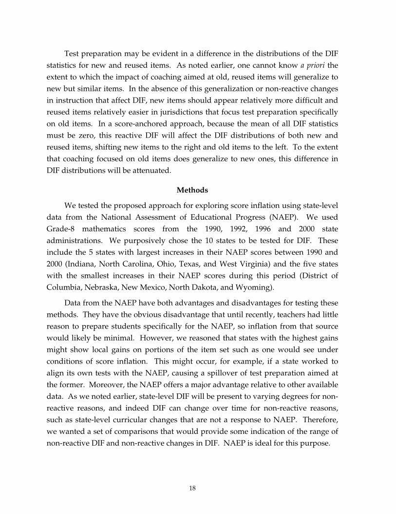
In practice, we found changes in SKEWDIF difficult to evaluate because skew was often influenced by a small number of outlier items. This was particularly true of Indiana, which showed a very large increase in the absolute value of SKEWDIF that stemmed in part from a three outliers in the year 2000 (Figure 4). Outliers had less extreme but appreciable effects in some other states as well. Nonetheless, given the exploratory purposes of this effort, it is worthwhile to explore the patterns show in our sample states.

25

1990 2000Year

-2

-1

0

1

DIF

Figure 4. Distributions of DIF in Indiana, 1990 and 2000 on theta scale.

No consistent change in the absolute magnitude of SKEWDIF was apparent in either group of states. Some states showed increases in the absolute amount of skew, while other showed decreases (Tables 3 and 4), and with the exception of Indiana, these changes were mostly modest.

Table 3

Changes in Absolute Magnitude of SKEWDIF in High-Gain States (in order of size of change)

WV -0.98 OH -0.54 NC 0.51 TX -0.01 IN 2.84

Mean 0.36

26

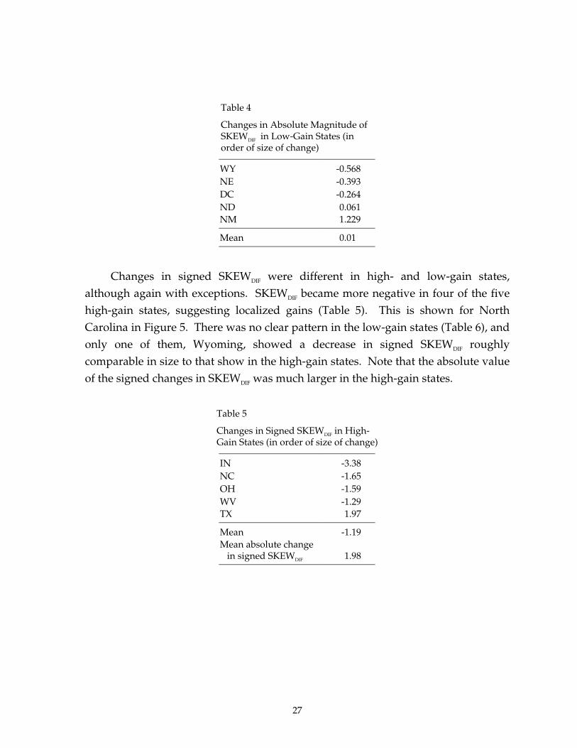
Table 4

Changes in Absolute Magnitude of SKEWDIF in Low-Gain States (in order of size of change)

WY -0.568 NE -0.393 DC -0.264 ND 0.061 NM 1.229

Mean 0.01

Changes in signed SKEWDIF were different in high- and low-gain states, although again with exceptions. SKEWDIF became more negative in four of the five high-gain states, suggesting localized gains (Table 5). This is shown for North Carolina in Figure 5. There was no clear pattern in the low-gain states (Table 6), and only one of them, Wyoming, showed a decrease in signed SKEWDIF roughly comparable in size to that show in the high-gain states. Note that the absolute value of the signed changes in SKEWDIF was much larger in the high-gain states.

Table 5

Changes in Signed SKEWDIF in High-Gain States (in order of size of change)

IN -3.38 NC -1.65 OH -1.59 WV -1.29 TX 1.97

Mean -1.19 Mean absolute change in signed SKEWDIF 1.98

27

-1.0 -0.5 0.0 0.5 1.0DIF

0

11

22

33

44

55

Cou

nt

-1.0 -0.5 0.0 0.5 1.0DIF

0

11

22

33

44

55

Cou

nt

Figure 5. Distributions of DIF in North Carolina, 1990 (solid line) and 2000 (dashed line), on theta scale (kernel smooths of histogram).

Table 6

Changes in Signed SKEWDIF in Low-Gain States (in order of size of change)

WY -1.23 NE -0.39 DC +0.59 ND +1.09 NM +1.51 Mean +0.31 Mean absolute change in signed SKEWDIF 0.96

Old and New Items

As noted earlier, test preparation focused on old test items could result in a difference in the DIF distributions of reused and new items. In a score-anchored method that constrains the overall mean DIF to be zero, this effect would appear in the locations of both DIF distributions: Old items would become relatively easier, and new items would be relatively harder. It will be attenuated to the extent that this preparation generalizes to similar new items, and it may be either attenuated or exacerbated by non-reactive changes in instruction.

28

To explore this, we used the results from our score-anchored DIF analysis, examining the distribution of the DIF statistic separately for new and reused items. For each focal state, the DIF distributions in the final year (2000) were examined for four groups of items: those used in all four assessments, those used in the three most recent, those used in the two most recent, and those used only in 2000. In addition, the DIF distributions in the 1992 and 1996 assessments were examined for items that were newly introduced in those years.

Despite the large number of comparisons (60 DIF distributions across the 10 states), very few of these distributions were centered at substantially non-zero values. Most of the means and medians were less than .05 in absolute value on the theta scale. There was some evidence of DIF affecting 1996 DIF distributions for items newly introduced in that year, but this DIF was apparently non-reactive, because it went in both directions and appeared in both low-and high-gain states.

The sole instance of DIF that conforms to the pattern one might find as a result of reactive DIF appeared in North Carolina (the state with the largest gains) in the 2000 assessment. It was the largest effect (that is, this DIF distribution was centered farther form zero than any other), but given that it appeared only in a single assessment in a single state, it would be risky to interpret it as evidence of reactive DIF. In 2000, the DIF distribution was shifted to the right (that is, new items were relatively harder) compared to all three sets of reused items. The distributions of 2000 DIF for the oldest items (used in all four assessments) and the items introduced in 2000 is shown in Figure 6. Note that the difference between the distributions stems from the smaller percentage of relatively easy items in the distribution of DIF in the newly introduced items.

Discussion

This study was exploratory in purpose, intended to develop an extension of DIF for analysis of cohort-to-cohort change and to probe the possible utility of this approach to the investigation of score inflation. Although the NAEP data used here were in some respects less than ideal for this purpose, the study does offer some suggestive results relevant to applications to data from higher-stakes state assessments.

29

-0.6 -0.3 0.0 0.3 0.6DIF in 2000

0

4

8C

ount

-0.6 -0.3 0.0 0.3 0.6DIF in 2000

0

4

8C

ount

Cou

nt

Figure 6. Distributions of in DIF in North Carolina, 2000, items used since 1990 (solid line) and items new in 2000 (dashed line), on theta scale (kernel smooths of histogram).

The findings suggest that variations in non-reactive DIF can be large. In this study, baseline SDDIF ranged from a low of .11 on the theta scale in Indiana to a high of .26 in the District of Columbia. Analyses of possible score inflation are likely to focus on differences among schools or districts within states rather than between states, and it is possible that between-group variations in curricular match may be smaller within states than between. Nonetheless, this finding suggests that it is important to examine baseline distributions of DIF empirically before estimating possibly reactive changes in DIF over time. Most extant evaluations of high-stakes testing have reconstructed data retrospectively (see, e.g., Klein et al., 2000; Koretz & Barron, 1998; Koretz et al., 1991), and the item-level data required for DIF analysis may be difficult to obtain years after administration.

The findings of this effort do not clearly indicate how fruitful comparisons of the DIF distributions of new and reused items will prove. The highest gain state, North Carolina, did yield one clear contrast between new and reused items, but neither other comparisons in North Carolina nor comparisons in other states showed sizable differences between the two. The dearth of substantial differences could reflect either of two factors. It may represent a lack of substantial test preparation

30

targeted specifically at previously used items in NAEP, or it may stem from generalization of the effects of such preparation to new but similar items. It would be valuable to test this approach next in the context of high-stakes testing programs in which preparation aimed at previously used items is widespread.

Two of the findings of this study suggest substantial obstacles to the application of these methods. The first is the finding of items that are outliers in the distribution of DIF. As a general rule, excluding outliers from analysis would seem to be the wrong response. First, the large DIF shown by these items may reflect precisely the types of preparation that are at issue. Second, the generally modest number of items in state testing programs would make the deletion of outliers analytically very costly. Addressing this problem will require qualitative analysis of the particular items involved.

The second discouraging result is the unanticipated finding that SDDIF increased appreciably in most of our 10 sampled states, including most of those that showed small gains in scores. In the case of NAEP, one can assume that low-gain states did not experience appreciable pressure to prepare students specifically for the NAEP, and thus low-gain states provide an indication of changes in non-reactive DIF. Therefore, this finding suggests that the assumption of reasonably stable non-reactive DIF is unwarranted. In the context of high-stakes testing programs, it is often the case that all or nearly all districts and schools face incentives to prepare specifically for the test, albeit to varying degrees, so no schools can provide a clear indication of non-reactive changes in DIF. Nonetheless, the contrast between high- and low-gain schools may be useful in this respect. One might assume that teachers in low-gain schools either responded less to the incentive to prepare specifically for the test or prepared less effectively, and therefore changes in DIF in low-gain schools may reflect less reactive DIF than changes in high-gain schools. For an example of comparisons of high- and low-gain schools without a formal DIF analysis, see Koretz and Barron (1998).

As a next step, these methods should be extended and further evaluated in the context of higher stakes testing programs. A logical next step would be to couple these methods with qualitative analysis of test items. This may help explain outlier items and distinguish between reactive and non-reactive DIF. For example, it would be informative to see whether items that show large negative DIF in settings with unusually high gains—that is, items that are relatively easy in those contexts—show recurrent patterns of content, presentation, or task demands. For examples of early

31

attempts to do this, see Koretz and Barron (1998), pp. 101-109. One could also classify items a priori in terms of characteristics relevant to potential inflation, such as similarity to previously used items, and separately examine the DIF distributions of those items. It would also be informative to examine the degree to which the same items show DIF consistently across small groups, such as schools, although this would require some methodological changes because of small counts.

32

References

Angoff, W. H. (1993). Perspectives on differential item functioning methodology. In P. W. Holland and H. Wainer (Eds.), Differential item functioning (pp. 3-24). Hillsdale, NJ: Lawrence Erlbaum Associates.

Bock, D., & Zimowski, M. (2003a). BILOG-MG examples. In M. du Toit (Ed.), IRT from SSI (pp. 634-691). Chicago: Scientific Software International.

Bock, D., & Zimowski, M. (2003b). Models in BILOG-MG. In M. du Toit (Ed.), IRT from SSI (pp. 530-543). Chicago: Scientific Software International.

Camilli, G., & Shepard, L. A. (1994). Methods for identifying biased rest items. Thousand Oaks, CA: Sage Publications.

Holland, P. W., & Wainer, H. (Eds.). (1993). Differential item functioning. Hillsdale, NJ: Lawrence Erlbaum Associates.

Jacob, B. (2002). Accountability, incentives and behavior: The impact of high-stakes testing in the Chicago Public Schools (Working Paper W8968). Cambridge, MA: National Bureau of Economic Research.

King, G., Murray, C. J. L., Salomon, J. A., & Tandon, A. (2004). Enhancing the validity and cross-cultural comparability of measurement in survey research. American Political Science Review, 98, 191-207.

Klein, S. P., Hamilton, L. S., McCaffrey, D. F., & Stecher, B. M. (2000). What do test scores in Texas tell us? (Issue Paper IP-202) Santa Monica, CA: RAND.

Koretz, D. (2002). Limitations in the use of achievement tests as measures of educators productivity. In E. Hanushek, J. Heckman, & D. Neal (Eds.), Designing incentives to promote human capital [Special issue]. The Journal of Human Resources, 37, pp. 752-777.

Koretz, D., & Barron, S. I. (1998). The validity of gains on the Kentucky Instructional Results Information System (KIRIS; MR-1014-EDU). Santa Monica, CA: RAND.

Koretz, D., Linn, R. L., Dunbar, S. B., & Shepard, L. A. (1991, April). The effects of high-stakes testing: Preliminary evidence about generalization across tests. In R. L. Linn (Chair), The effects of high stakes testing. Symposium presented at the annual meetings of the American Educational Research Association and the National Council on Measurement in Education, Chicago.

Koretz, D., McCaffrey, D., & Hamilton, L. (2001). Toward a framework for validating gains under high-stakes conditions. (CSE Technical Report No. 551). Los Angeles:

33

34

University of California, National Center for Research on Evaluation, Standards, and Student Testing (CRESST).

O’Connor, K. (2000). TIMSS field test. In M. O. Martin, K. D. Gregory, & S. E. Stemler, (Eds.), TIMSS 1999 technical report, (pp. 103-116). Chestnut Hill, MA: TIMSS International Study Center, Boston College.

Scientific Software International. (2003). BILOG-MG for Windows, Version 3.0.2327.2. Lincolnwood, IL: Author.

Thissen, D. (2003). MULTILOG examples. In M. du Toit (Ed.), IRT from SSI, Chapter 12. Chicago: Scientific Software International.

Thissen, D., Steinberg, L., & Wainer, H. (1993). Detection of differential item functioning using the parameters of item response models. In P. W. Holland & H. Wainer (Eds.), Differential item functioning (pp. 67-114). Hillsdale, NJ: Lawrence Erlbaum Associates.

Wang, W-C., & Yeh, Y-L. (2003). Effects of anchor item methods on differential item functioning detection with the likelihood ratio test. Applied Psychological Measurement, 27, 479-498.

Wolfe, R. G. (1997, March). Country-by-item interactions: Problems with content validity in Scaling. In Validity in cross-national assessments: Problems and pitfalls. Symposium presented at the annual meeting of the American Educational Research Association, Chicago.

Zwick, R. (1990). When do item response function and Mantel-Haenszel definitions of differential item functioning coincide? Journal of Educational Statistics, 15, 185-197.