i

Using Natural Language as Knowledge Representation

in an Intelligent Tutoring System

By

Sung-Young Jung

Bachelor, Korea Advanced Institute of Science and Technology, 1994

Master, Korea Advanced Institute of Science and Technology, 1996

Master, University of Pittsburgh, 2008

Submitted to the Graduate Faculty of

Intelligent Systems Program in partial fulfillment

of the requirements for the degree of

Doctor of Philosophy

University of Pittsburgh

2011

ii

UNIVERSITY OF PITTSBURGH

INTELLIGENT SYSTEMS PROGRAM

This dissertation was presented

by

Sung-Young Jung

It was defended on

August 29, 2011

and approved by

Kurt VanLehn, Professor, School of Computing, Info. and Decision Systems Eng., Arizona State University

Kevin D. Ashley, Professor, School of Law, University of Pittsburgh

Daqing He, Associate Professor, School of Information Sciences, University of Pittsburgh

Dissertation Director: Alan Lesgold, Professor, School of Education, University of Pittsburgh

iii

Copyright © by

Sung-Young Jung

2011

iv

Using Natural Language as Knowledge Representation

in an Intelligent Tutoring System

Sung-Young Jung, Ph.D.

University of Pittsburgh, 2011.

Knowledge used in an intelligent tutoring system to teach students is usually acquired from authors who

are experts in the domain. A problem is that they cannot directly add and update knowledge if they

don’t learn formal language used in the system. Using natural language to represent knowledge can

allow authors to update knowledge easily. This thesis presents a new approach to use unconstrained

natural language as knowledge representation for a physics tutoring system so that non-programmers

can add knowledge without learning a new knowledge representation. This approach allows domain

experts to add not only problem statements, but also background knowledge such as commonsense and

domain knowledge including principles in natural language. Rather than translating into a formal

language, natural language representation is directly used in inference so that domain experts can

understand the internal process, detect knowledge bugs, and revise the knowledgebase easily. In

authoring task studies with the new system based on this approach, it was shown that the size of added

knowledge was small enough for a domain expert to add, and converged to near zero as more problems

were added in one mental model test. After entering the no-new-knowledge state in the test, 5 out of

13 problems (38 percent) were automatically solved by the system without adding new knowledge.

v

TABLE OF CONTENTS

TABLE OF CONTENTS ..................................................................................................................................... v

PREFACE ...................................................................................................................................................... xii

1.0 INTRODUCTION ................................................................................................................................. 1

2.0 THE PREVIOUS ITS: PYRENEES ........................................................................................................... 3

2.1. FORMAL LANGUAGE REPRESENTATION OF PYRENEES ................................................................. 3

2.2. DIFFICULTIES IN AUTHORING IN FORMAL LANGUAGE ................................................................. 5

3.0. TYPES OF KNOWLEDGE IN THE THREE LEVELS IN PHYSICS ............................................................... 7

4.0. REPRESENTING KNOWLEDGE IN NATURAL LANGUAGE ................................................................... 8

4.1. REPRESENTING BACKGROUND KNOWLEDGE ............................................................................. 10

5.0. SYSTEM ARCHITECTURE OF NATURAL-K ......................................................................................... 12

6.0. TYPES OF KNOWLEDGE IN NATURAL-K ........................................................................................... 13

6.1. IMPLICATION RULES .................................................................................................................... 14

6.1.1. Default Rule ......................................................................................................................... 14

6.1.2. Negative condition, and Unknown condition ..................................................................... 15

6.1.3. Negation Rule ...................................................................................................................... 15

6.1.4. Principles ............................................................................................................................. 16

6.2. TRUTH RULES .............................................................................................................................. 16

6.2.1. Logic Rule ................................................................................................................................ 18

7.0. GENERALIZED REPRESENTATION .................................................................................................... 18

7.1. THE SHORTER, THE MORE GENERAL ........................................................................................... 19

7.2. USING SEMANTICALLY BINDING VARIABLES ............................................................................ 19

7.3. USING SEMANTICALLY BINDING PHRASE VARIABLES ............................................................. 20

8.0. REPRESENTING TIME ....................................................................................................................... 21

8.1. TIME INDEX: INTERNAL REPRESENTATION OF TIME ............................................................... 22

8.2. TIME VALUE ASSIGNMENT ........................................................................................................ 24

8.3. TIME PHRASE .............................................................................................................................. 25

9.0. REPRESENTING PHYSICS MENTAL MODELS .................................................................................... 27

9.1. A BASIC MENTAL MODEL ......................................................................................................... 28

9.2. MENTAL MODEL EXTENSION .................................................................................................... 29

vi

9.3. AN INFERENCE EXAMPLE ........................................................................................................... 32

10.0. INFERENCE .................................................................................................................................. 36

10.1. FORWARD AND BACKWARD CHAINING .................................................................................. 36

10.2. DEFAULT KNOWLEDGE INFERENCE ....................................................................................... 37

10.3. KNOWLEDGE SUBSUMPTION ................................................................................................. 38

10.4. INFERENCE WITH PHRASE VARIABLES .................................................................................. 39

10.5. INFERENCE WITH SYMBOLIC TIME INDEX ........................................................................... 40

11.0. NATURAL LANGUAGE AS KNOWLEDGE REPRESENTATION ..................................................... 40

11.1. USING UNCONSTRAINED NATURAL LANGUAGE .................................................................. 43

11.2. INTERNAL REPRESENTATION OF A SENTENCE ....................................................................... 45

11.3. AMBIGUITY .............................................................................................................................. 45

11.3.1. Syntactic Ambiguity............................................................................................................. 45

11.3.2. Semantic Ambiguity ............................................................................................................ 46

11.4. SYNTACTIC NORMALIZATION ................................................................................................. 47

11.4.1. Active vs. Passive Voice (does vs. is done) .......................................................................... 47

11.4.2. Relative Clause (A which B) ................................................................................................. 47

11.4.3. Conjunctive phrase (A and B) .............................................................................................. 48

11.4.4. Inserting a Normalization Link to Chart .............................................................................. 48

11.5. PRONOUN RESOLUTION......................................................................................................... 49

11.6. MATCHING TWO SENTENCES ................................................................................................ 50

12.0. STUIDES AND RESULTS ................................................................................................................ 51

12.1. GOALS AND EVALUATION PLAN .............................................................................................. 51

12.2. Knowledge Adding Task .......................................................................................................... 52

12.3. Rewording Task ....................................................................................................................... 57

12.4. The Number of Mental Models............................................................................................... 58

12.5. STUDIES WITH RECRUITED USERS ........................................................................................... 60

13. DISCUSSION ..................................................................................................................................... 65

13.1. CONVERGENCE OF THE AMOUNT OF KNOWLEDGE TO ADD ................................................. 66

13.2. A New Dimension of ITS Types................................................................................................ 68

13.3. Separating Knowledge from Computer Programming ........................................................... 68

13.4. THE ISSUE OF MENTAL MODELS .......................................................................................... 69

13.5. THE AMBIGUITY ISSUE........................................................................................................... 70

vii

13.6. THE OVER-GENERATION ISSUE ............................................................................................... 71

13.7. GENERATING HINTS AND EXPLANATIONS FOR TUTORING .................................................... 72

13.8. A NEW KIND OF INTELLIGENT TUTORING SYSTEMS ............................................................... 74

13.8.1. An ITS for Problem Understanding ..................................................................................... 74

13.8.2. A Teachable Agent .............................................................................................................. 75

13.8.3. Application to the Law Domain ........................................................................................... 76

13.9. FEASIBILITY ISSUES .................................................................................................................. 77

13.9.1. System-determined vs. User-determined Knowledge Space ............................................. 77

13.9.2. The Issue of Commonsense Knowledge ............................................................................. 79

13.9.3. The Issue of Paraphrases .................................................................................................... 80

13.10. WHAT IS NEW IN THE THESIS? ................................................................................................ 80

13.11. WHY HASN’T IT BEEN DONE BEFORE? .................................................................................... 82

13.12. FUTURE WORK ........................................................................................................................ 83

13.12.1. Rule generalization ......................................................................................................... 83

13.12.2. More Natural Representation ......................................................................................... 83

13.12.3. Where Can We Go Further? ............................................................................................ 84

CONCLUSIONS ............................................................................................................................................. 85

BIBLIOGRAPHY ............................................................................................................................................ 86

viii

LIST OF FIGURES

Figure 1: The problem statement of the Skateboarder problem ................................................................. 3

Figure 2: Predicates defining a principle, Projection. ................................................................................... 4

Figure 3: A statement of the Skateboarder problem represented in formal language ................................ 4

Figure 4: the generated equation for the skateboarder problem ................................................................ 5

Figure 5: (a) physics representation and (b) math of the skateboarder problem. ....................................... 7

Figure 6: formal and natural language representations of the skateboarder problem. .............................. 9

Figure 7: the projection principle represented in formal language and natural language........................... 9

Figure 8: background knowledge translating the input sentences into physics representations. ............. 11

Figure 9: The five types of knowledge represented in natural language, and their data flow during

problem solving........................................................................................................................................... 12

Figure 10: the system architecture of Natural-K ........................................................................................ 13

Figure 11: the basic form of an implication rule ......................................................................................... 14

Figure 12: examples of default rules ........................................................................................................... 14

Figure 13: An example for positive and negative facts, and positive, negative, and unknown conditions 15

Figure 14: an example of negation rule (A does not imply B). ................................................................... 15

Figure 15: the basic form of a principle ...................................................................................................... 16

Figure 16: the basic from of a truth rule ..................................................................................................... 16

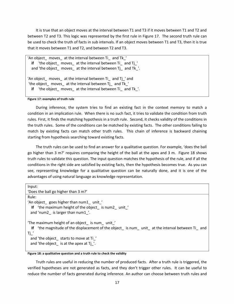
Figure 17: examples of truth rule ............................................................................................................... 17

Figure 18: a qualitative question and a truth rule to check the validity ..................................................... 17

Figure 19: examples of truth rule for logic and math ................................................................................. 18

Figure 20: an example sentence and a truth rule for math to calculate the actual direction (35+90

degrees) ...................................................................................................................................................... 18

Figure 21: generalizing by making shorter .................................................................................................. 19

Figure 22: predefined semantically binding variables ................................................................................ 20

Figure 23: example rules using semantically binding phrase variables ...................................................... 20

Figure 24: a fact with a time point .............................................................................................................. 21

Figure 25: Problem statement of throwing upward ................................................................................... 21

Figure 26: creating a new time point .......................................................................................................... 22

Figure 27: The form of time index and examples. ...................................................................................... 22

Figure 28: creating a new time interval ...................................................................................................... 23

Figure 29: generated facts with a time index assigned .............................................................................. 23

Figure 30: an example with two time intervals .......................................................................................... 23

Figure 31: Time index and time value assignment ..................................................................................... 24

Figure 32: The generated facts with a final time value assigned. ............................................................... 24

Figure 33: Time index and time value assignment when two time intervals are given. ............................ 24

Figure 34: a sentence with a conjunctive time phrase, and a rule to recognize it ..................................... 25

Figure 35: an example of to-infinite time phrase, and a rule to interpret ................................................. 25

Figure 36: an example of adjective time phrase (initial~, final~, whole~, total~), and rules to interpret .. 26

Figure 37: types of time phrases, and corresponding rules to interpret them .......................................... 26

ix

Figure 38: a mental model for projectile movement represented in formal language in Pyrenees .......... 27

Figure 39: the basic mental model for throwing upward ........................................................................... 28

Figure 40: a rule for starting movement ..................................................................................................... 28

Figure 41: a rule for movement at the interval and the final event ........................................................... 29

Figure 42: a rule for the event returning to the initial level of height ........................................................ 29

Figure 43: generated facts with a time index ............................................................................................. 29

Figure 44: generate facts with a time point ................................................................................................ 29

Figure 45: throwing upward on a high place .............................................................................................. 30

Figure 46: the background rule for throwing upward in a high place. ....................................................... 30

Figure 47: a logic rule to generate a mid time point. ................................................................................. 30

Figure 48: throwing upward and reaching the apex ................................................................................... 31

Figure 49: the mental model extension rule for reaching the apex ........................................................... 31

Figure 50: A ring thrown upward from the roof of a building .................................................................... 31

Figure 51: a background rule for the apex .................................................................................................. 31

Figure 52: two principles for the throwing-upward mental model. (a) Initial and final velocities (b)

displacement and initial velocity ................................................................................................................ 32

Figure 53: generated facts by the basic mental model .............................................................................. 32

Figure 54: generated facts by the extended mental model ....................................................................... 33

Figure 55: generated facts by the extended mental model for reaching the apex .................................... 33

Figure 56: background rules for the last two questions ............................................................................. 33

Figure 57: the two questioned translated in physics representation ......................................................... 33

Figure 58: the produced facts with time index attached ............................................................................ 34

Figure 59: generated facts at the end of the inference stage .................................................................... 35

Figure 60: generated equations .................................................................................................................. 35

Figure 61: the output of the equation solver ............................................................................................. 35

Figure 62: The final answers generated ...................................................................................................... 35

Figure 63: an example of default knowledge that can generate different results depending on application

order ........................................................................................................................................................... 38

Figure 64: over-generation example (an input sentence, two rules, and the two facts generated).......... 38

Figure 65: Subsumption relations drawn as directed graph ....................................................................... 39

Figure 66: an example of inference failure due to a time phrase .............................................................. 39

Figure 67: a background rule inferring projectile movement ..................................................................... 40

Figure 68: an example of syntactic ambiguity (prepositional attachment). (a) an input sentence (b) two

interpretations in formal language. ............................................................................................................ 42

Figure 69: Ambiguity resolution in the natural language representation (a) the input sentence followed

by another sentence (b) a background rule to infer that the airplane was on the hill (c) another example

of the input sentence followed by another sentence (d) a background rule to infer that the man was on

the hill. ........................................................................................................................................................ 42

Figure 70: Previous approaches to transform natural language to formal language ................................. 43

Figure 71: knowledge in unconstrained natural language ......................................................................... 44

Figure 72: accepting ungrammatical input. (a) an ungrammatical sentence (b) a rule to accept it. ......... 44

x

Figure 73: A chart containing all parse trees generated is used as internal representation of a sentence.

.................................................................................................................................................................... 46

Figure 74: Syntactic normalization of a passive form ................................................................................. 47

Figure 75: a relative clause and its variation .............................................................................................. 48

Figure 76: sentence normalization for relative clause ................................................................................ 48

Figure 77: Sentence normalization for conjunctive phrase. ....................................................................... 48

Figure 78: A normalization link in a least common ancestor (LCA)=’pushed’. (a) The LCA of ‘pushed’ and

‘man’ is ‘pushed’. So activate the link (b) the LCA of ‘pushed’ and ‘man’ is ‘was’. So inactivate the link.. 49

Figure 79: a background rule designating a physics object. ....................................................................... 49

Figure 80: (a) an example of a pronoun in which recency heuristics fails, (b) a background rule required

to resolve the pronoun ‘it’ .......................................................................................................................... 50

Figure 81: an example of background rule with a pronoun ‘it’ .................................................................. 50

Figure 82: the number of rules added for each physics problem in Pyrenees ........................................... 53

Figure 83: the number of rules added for each physics problem in Young&Freeman’s Textbook ............ 54

Figure 84: the number of background rules added for each physics problem in Throw-upward mental

model .......................................................................................................................................................... 55

Figure 85: reasons of the added rules for the problems in the throw-upward mental model (a) for a

mental model (b) for time phrases (c) for paraphrases (d) for questions. ................................................. 56

Figure 86: an example of rewording. (a) An original problem statement (b) a reworded statement (c) the

number of edits ((w) is a deletion, (w1->w2) is a modification, and the others are addition) .................. 58

Figure 87: The min-edit distance after the tenth problem (total 13 problems). ........................................ 58

Figure 88: the number of mental models in each of three chapters in Young and Freedman’s textbook. 59

Figure 89: An example of (a) a problem statement, (b) a reworded statement, and (c) added rules by the

subject4 ....................................................................................................................................................... 61

Figure 90: The min-edit distance for each of the recruited subjects .......................................................... 62

Figure 91: The number of rules added by each subject .............................................................................. 63

Figure 92: The min-edit distance, time spent, and the number of trials in average across the subjects. .. 63

Figure 93: The number of rules added, time spent, and the number of trials in average across subjects 64

Figure 94: Question1 ................................................................................................................................... 64

Figure 95: Question2 ................................................................................................................................... 65

Figure 96: Question3 ................................................................................................................................... 65

Figure 97: The main two factors determining convergence of the size of required knowledge. ............... 66

Figure 98: comparison of three types of tutoring systems and the size of knowledge to add. ................. 67

Figure 99: A new dimension of ITS types .................................................................................................... 68

Figure 100: Examples to deal with ambiguity: (a) an input sentence (b) an over-generated case due to

the prepositional attachment (c) removing the over-generated output by rewriting the rule to be more

specific (d) removing the over-generated output by copy-and-pasting the input sentence to the rule. .. 70

Figure 101: Inference log of the case1 of Figure 100 ................................................................................. 71

Figure 102: over-generation example ......................................................................................................... 71

Figure 103: the problem statement of Balloon Problem ............................................................................ 72

Figure 104: An example generating hits ..................................................................................................... 73

Figure 105: An example generating explanations ...................................................................................... 73

xi

Figure 106: inference steps of the Balloon problem. ................................................................................. 73

Figure 107: background knowledge for the balloon example .................................................................... 74

Figure 108: An example of an ITS helping a student how to understand the Balloon problem (Figure 103).

.................................................................................................................................................................... 75

Figure 109: the process of student’s adding the skateboarder problem to the system. ........................... 76

Figure 110: An example of an article (a) in a law book (b) in a form of rule .............................................. 76

Figure 111: An example of a bill of indictment ........................................................................................... 77

Figure 112: an example of background knowledge to interpret the bill of indictment ............................. 77

Figure 113: a generated fact ....................................................................................................................... 77

Figure 114: The final sentence generated .................................................................................................. 77

Figure 115: examples of paraphrase ........................................................................................................... 80

Figure 116: semantically binding variables with an underbar (upper) and without an underbar (lower) . 84

xii

PREFACE

This dissertation was possible by the full support of my advisor Dr. Kurt VanLehn who inspired me to go

deep into the core problem of artificial intelligence that was believed to be infeasible for a long time. It

required big ambition, courage, and adventurous spirit to break through the barriers in the land where

no one has ever set foot. During this research, I got convinced that artificial intelligence was around the

corner. I hope that this dissertation helps readers to share my experiences and to have courage to go

for the dream. I also want to thank Dr. Alan Lesgold, Dr. Kevin Ashley, and Dr. Daqing He for giving me

invaluable comments and advice.

1

1.0 INTRODUCTION An Intelligent Tutoring System (ITS) can teach students to learn and acquire domain knowledge provided

by the system, and the system needs to acquire such knowledge from authors who are domain experts

(Murray, 2003). Although one might be able to team a domain expert with a programmer for the initial

development of such a system, that approach is not sustainable. For example, high school teachers who

don’t know computer programming and a formal language may want to add new domain problems to

use in their class. Moreover, different teachers have different directions and preferences on class

materials, and would like an ITS to which they can add their own domain problems for their class.

During the authoring process, authors should be able to follow each step of the problem solving,

detect errors, and fix them by adding and updating knowledge. They may not be able to do such tasks if

the knowledge is represented in formal language. Although it is possible that the system generates

natural language explanations of its reasoning from the formal language, domain experts still cannot

edit the knowledge directly. This suggests developing a system using natural language to represent

knowledge so that non-programmers can easily develop and maintain ITS knowledge.

The thesis addresses mainly a goal to find a way to represent required background knowledge in

natural language so that the system can understand a problem statement and solve it like a student can

read and solve it. The other goal is to find a way to represent generalized knowledge in natural

language so that the size of knowledge which domain experts have to add decreases as more problems

are added, and converges to near zero. All the other knowledge that the ITS needs, e.g., in order to

solve problems and coach students during problem solving, is built into the ITS in a domain-general

fashion, so that authors need never examine it nor debug it. In short, the proposed system is intended

primarily for use by domain experts to add domain problems to an existing ITS. It can also be used to

add domain problems to an initially empty ITS, but that usage is secondary.

Some studies of applying natural language understanding to tutoring systems were performed

before. Novak developed a physics problem solving system, ISAAC, that reads a problem statement

written in natural language and solved the given problem (Novak Jr., 1977). ISAAC received natural

language input and transformed it into semantic frames which were a kind of formal representation. A

physics problem solver, MECHO (Bundy, Byrd, Luger, Mellish, & Palmer, 1979), also transformed a

problem statement into formal language.

These and other studies evaluated the potential of the idea adopting natural language as input

form of knowledge for problem statements. However, the advantage was limited because background

knowledge such as commonsense knowledge had to be encoded inside program routines. Only

computer programmers were able to update such knowledge. So, adding a new domain problem was

limited to cases where all required background knowledge was already encoded in the systems. If a

domain problem failed to be translated properly or the background knowledge was incomplete, then

the author had no easy way to fix or even understand the flaw. This suggests that authors must be able

to read and edit the background knowledge as well as the problem statements.

2

Acquiring knowledge from natural language is an old idea in the natural language processing area.

A common approach in this idea was to transform natural language into formal representations such as

logic forms (Jurafsky & Martin, 2000)(Brachman & Levesque, 2004) or semantic networks (Sowa,

1990)(Shastri, 1990). Using precise formal representations after transformation, the systems performed

inference to accomplish a goal. In modern work on knowledge capture and knowledge acquisition,

formal language was commonly used to represent knowledge in systems such as KANTOO(Nyberg,

Mitamura, & Betteridge, 2005), KAT (Moldovan, Girju, & Rus, 2000.), and WordNet2 (Harabagiu, Miller,

& Moldovan, 1999). In other systems, such as AURA (Chaudhri, John, Mishra, Pacheco, Porter, &

Spaulding, 2007) and SHAKEN (Clark, et al., 2001), domain experts transformed contents of science

textbook to graphical notations which is another form of formal language. The main problem of this

approach was that still only knowledge engineers and programmers could update the formal language

when update is needed, and knowledge required for transformation (such as templates) was implicitly

encoded in program code, thus also only programmers could update it.

Another direction comparable to this thesis is to use natural language to represent logic. There

have been several such studies. For instance, Natural Logic is an approach to recognize textual

entailment (MacCartney & Manning, 2008). Controlled Natural Language restricts natural language

syntax to use English as formal language (Fuchs, Kaljurand, & Kuhn, 2008). Logic-oriented studies mainly

focus on obtaining sound logical inferences rather than expediting knowledge acquisition. A problem in

this approach rises when some knowledge cannot be represented in given constraints. Then again, only

programmers can change the constraints.

A common issue in the previous studies was that using natural language in knowledge

representation requires a proper way to deal with commonsense knowledge. One of the problems

known in this approach is that there can be million different natural language expressions for the same

element of underlying knowledge and there is no easy way to recognize them. This is called the

paraphrasing problem. Textual entailment is an area dedicated to find a way for this problem. For

example, “the force applied to the object” textually entails “the force exerted to the object”. Using

enough background knowledge has been recognized as one of the most important factors in the textual

entailment (Iftene, 2009).

As the needs for commonsense knowledge increased in many AI systems, attempts to build

commonsense knowledge base started, such as Opencyc (OpenCyc Tutorial), Learner (Chklovski, 2003),

OpenMind (Speer, 2007), MindNet (Dolan & Richardson, 1996), and TextNet (Harabagiu & Moldovan,

1994). They try to build a universal commonsense knowledgebase represented in formal language.

However, it is unlikely that the complete set of universal commonsense knowledge can be built soon.

Such resources were not used in this thesis because what we need is a small set of knowledge required

to solve a given domain problem rather than the complete set of universal knowledge.

A dilemma of knowledge representation in natural language was that commonsense knowledge

was needed but it was not available. A basic approach for this issue is that commonsense knowledge

can be acquired in natural language from authors too. Because an ITS is task specific, it is hypothesized

that the amount of knowledge to add per a problem is feasibly small for an author to add in an ITS. The

3

validity of this hypothesis will be tested by authoring physics problems from textbooks in studies

(section 12.2).

This thesis presents a way to allow authors to add not only problem statements, but also

background knowledge including commonsense and domain knowledge. The main approach is to use

unconstrained natural language to represent knowledge so that authors can understand knowledge, add

knowledge, detect bugs, and fix them easily.

2.0 THE PREVIOUS ITS: PYRENEES The previous ITS, Pyrenees is presented here shortly to demonstrate the problems and difficulties clearly.

The new system Natural-K will be presented later, and it was driven from Pyrenees to overcome the

difficulties.

2.1. FORMAL LANGUAGE REPRESENTATION OF PYRENEES Pyrenees is a model-tracing tutoring system for equation-based problems. It teaches students both the

principles themselves and how to apply them to solve a problem efficiently. All of its pedagogical

knowledge is hardwired into it, so the author need only provide the domain knowledge. Although it has

been used with several task domains (including thermodynamics, statistics and microeconomics),

introductory mechanics is the target domain. Domain knowledge in Pyrenees includes a set of problems,

a set of principles and ontology. Problems are solved by finding a relevant set of equations then solving

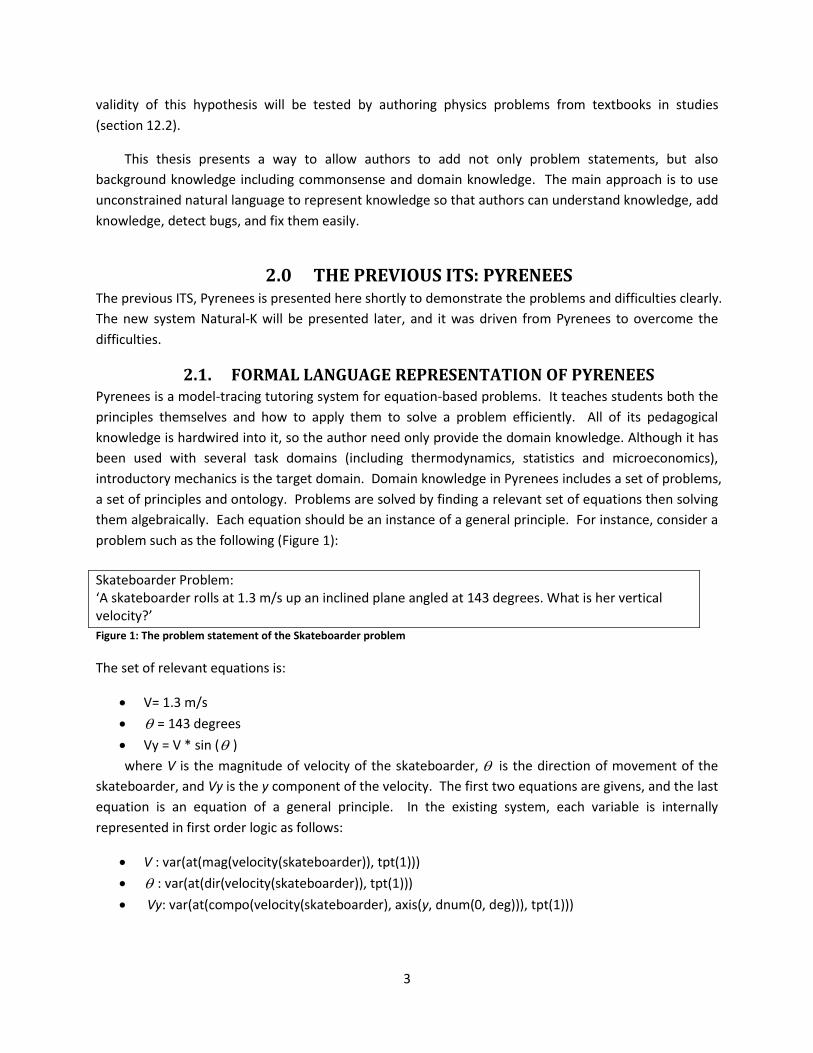
them algebraically. Each equation should be an instance of a general principle. For instance, consider a

problem such as the following (Figure 1):

Figure 1: The problem statement of the Skateboarder problem

The set of relevant equations is:

V= 1.3 m/s

= 143 degrees

Vy = V * sin ( )

where V is the magnitude of velocity of the skateboarder, is the direction of movement of the

skateboarder, and Vy is the y component of the velocity. The first two equations are givens, and the last

equation is an equation of a general principle. In the existing system, each variable is internally

represented in first order logic as follows:

V : var(at(mag(velocity(skateboarder)), tpt(1)))

: var(at(dir(velocity(skateboarder)), tpt(1)))

Vy: var(at(compo(velocity(skateboarder), axis(y, dnum(0, deg))), tpt(1)))

Skateboarder Problem: ‘A skateboarder rolls at 1.3 m/s up an inclined plane angled at 143 degrees. What is her vertical velocity?’

4

This says, for instance, that Vy is a variable (var) denoting the value at time point 1 (tpt(1)) of the

component (compo) along the y-axis of an unrotated coordinate system (axis(y,dnum(0,deg))) of the

velocity of the skateboarder.

There are three domain knowledge bases: ontology, principles, and problems. The ontology

describes the domain objects, properties and relationships, as well as how to translate

each formal term into English. For instance, the ontology would indicate that skateboarder is

an object, that at(mag(velocity(skateboarder)), tpt(1)) is a quantitative property, and that

var(at(mag(velocity(skateboarder)), tpt(1))) is an algebraic variable for that quantitative property.

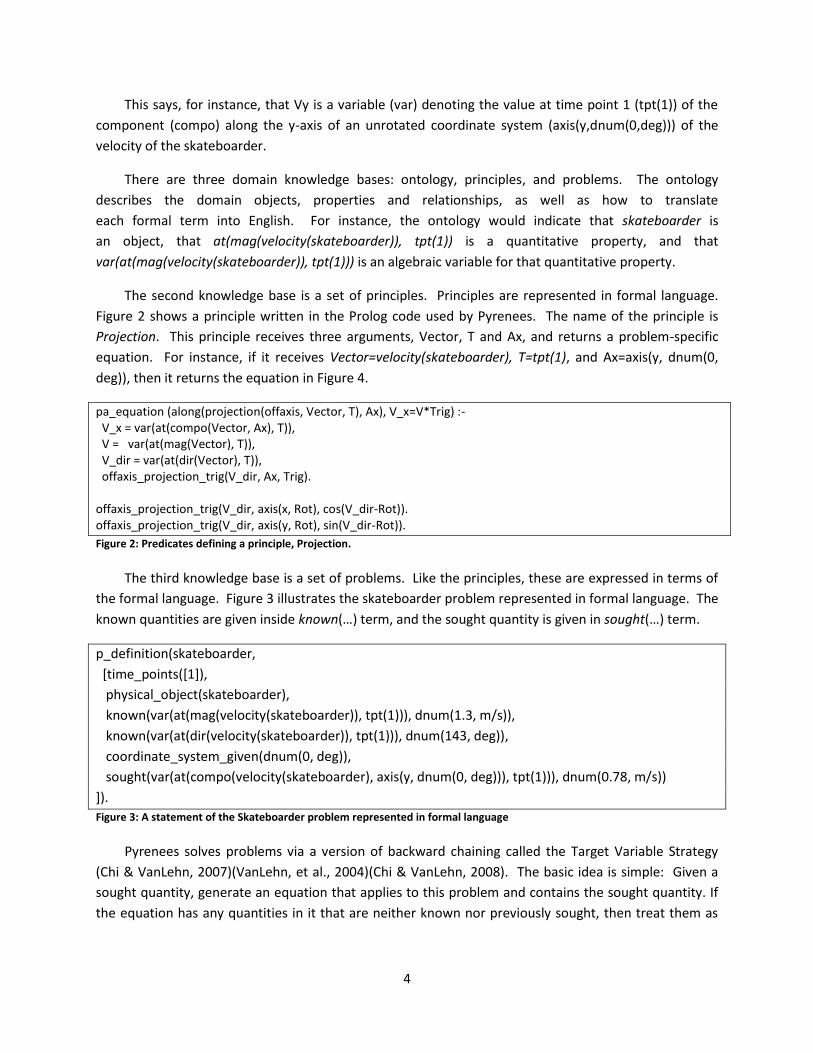
The second knowledge base is a set of principles. Principles are represented in formal language.

Figure 2 shows a principle written in the Prolog code used by Pyrenees. The name of the principle is

Projection. This principle receives three arguments, Vector, T and Ax, and returns a problem-specific

equation. For instance, if it receives Vector=velocity(skateboarder), T=tpt(1), and Ax=axis(y, dnum(0,

deg)), then it returns the equation in Figure 4.

pa_equation (along(projection(offaxis, Vector, T), Ax), V_x=V*Trig) :- V_x = var(at(compo(Vector, Ax), T)), V = var(at(mag(Vector), T)), V_dir = var(at(dir(Vector), T)), offaxis_projection_trig(V_dir, Ax, Trig). offaxis_projection_trig(V_dir, axis(x, Rot), cos(V_dir-Rot)). offaxis_projection_trig(V_dir, axis(y, Rot), sin(V_dir-Rot)). Figure 2: Predicates defining a principle, Projection.

The third knowledge base is a set of problems. Like the principles, these are expressed in terms of

the formal language. Figure 3 illustrates the skateboarder problem represented in formal language. The

known quantities are given inside known(…) term, and the sought quantity is given in sought(…) term.

p_definition(skateboarder,

[time_points([1]),

physical_object(skateboarder),

known(var(at(mag(velocity(skateboarder)), tpt(1))), dnum(1.3, m/s)),

known(var(at(dir(velocity(skateboarder)), tpt(1))), dnum(143, deg)),

coordinate_system_given(dnum(0, deg)),

sought(var(at(compo(velocity(skateboarder), axis(y, dnum(0, deg))), tpt(1))), dnum(0.78, m/s))

]).

Figure 3: A statement of the Skateboarder problem represented in formal language

Pyrenees solves problems via a version of backward chaining called the Target Variable Strategy

(Chi & VanLehn, 2007)(VanLehn, et al., 2004)(Chi & VanLehn, 2008). The basic idea is simple: Given a

sought quantity, generate an equation that applies to this problem and contains the sought quantity. If

the equation has any quantities in it that are neither known nor previously sought, then treat them as

5

sought and recur. When the Target Variable Strategy stops, it has generated a set of equations that are

guaranteed to be solvable.

In the case of the problem above, the Pyrenees would start with the variable

var(at(compo(velocity(skateboarder), axis(y, dnum(0, deg))), tpt(1))) as the sought quantity. It then

checks all its principles, and finds that the principle in Figure 2 has a term in its equation that unifies

with the variable. This unification binds Vector to velocity(skateboarder), T to tpt(1), and Ax to axis(y,

dnum(0, deg)) and creates the equation as Figure 4.

var(at(compo(velocity(skateboarder), axis(y, dnum(0, deg))), tpt(1))) = var(at(mag(velocity(skateboarder)), tpt(1))) * sin(var(at(dir(velocity(skateboarder)), tpt(1)))-0). Figure 4: the generated equation for the skateboarder problem

Pyrenees notes that the equation has two quantities in it. The first is

var(at(mag(velocity(skateboarder)), tpt(1))). It checks the problem statement, and discovers that this

quantity is known, so it does not need to recursively seek a value for it. It now consider the second

quantity in the equation, var(at(dir(velocity(skateboarder)), tpt(1))). That too is known, so Pyrenees is

done with this problem, having “written” just one equation.

The take-home message of this section is that even though the skateboarder problem (Figure 1) is

extremely simple, the formality of the knowledge used to represent and solve it would be a serious

impediment to an author who has neither the time, skills, or inclination to master it.

2.2. DIFFICULTIES IN AUTHORING IN FORMAL LANGUAGE The first obvious difficulty in authoring Pyrenees is in understandability. Let’s take a look at the sought

quantity again.

var(at(compo(velocity(skateboarder), axis(y, dnum(0, deg))), tpt(1)))

It is unrealistic to expect that domain experts can easily understand and write such quantities

represented in formal language. So, they cannot participate in authoring using this representation. Also,

it is difficult to read even for a knowledge engineer. The second difficulty in authoring is in parenthesis.

In a case where a knowledge engineer writes the quantity in formal language, the mis-matching

parenthesis is a frequent source of mistakes and errors. Syntax directed editors will balance the

parentheses, but they may not know the argument structure of the knowledge representation, which

makes mismatching parentheses hard to detect. The first line below is wrong and the second is correct,

but they are hard to tell apart:

var(at(compo(velocity(skateboarder), axis(y, dnum(0, deg)), tpt(1))))

var(at(compo(velocity(skateboarder), axis(y, dnum(0, deg))), tpt(1)))

Humans can understand and communicate without parenthesis using natural language. A natural

language sentence looks simpler and easier, and the chance of writing an error is much smaller without

parenthesis. Let’s look at the variable represented in natural language and compare it to the above

formal version to see how easily authors can understand.

6

“The vertical velocity of the skateboarder at T1”

The third difficulty is in the strict argument ordering of formal language. Each of arguments should

be given in predetermined order. An author should remember the order and the required set of

arguments for each quantity. Following are simplified examples for force. There can be different

argument orders and all of them except one are errors to the system. The author should remember the

right order of arguments for each quantity, and it is a big burden.

force(agent, object, applied) : correct

force(object, agent, applied) : incorrect

force(agent, applied, object) : incorrect

force(object, applied, agent) : incorrect

In the case of natural language representation, syntactic constraints using prepositions have a role

in determining arguments. It is naturally understood by authors, and the system also can accept them

without a big difficulty.

“The applied force exerted to the object by the agent”

“The force applied to the object by the agent”

“The force applied by the agent to object”

It is possible to display quantities in natural language from the formal language using a generation

module, but domain experts still cannot edit them directly.

In previous approaches, it was common to use natural language for authors and transform to

formal language for a system. However, transforming between natural and formal languages had many

problems such as lack of flexibility, extensibility, and difficulty in managing commonsense knowledge,

etc. Basically, the difficulties were from the situation that programmers had to change transformation

modules containing transformation knowledge whenever a new pattern of knowledge should be added.

The idea presented in this thesis is to use natural language directly without transforming to formal

language to avoid such difficulties.

Natural language representation is more easily learned than formal language, which lowers the

barriers for instructors and even students to add knowledge to the ITS. Besides understandability and

learnability, natural language allows the problem solver’s reasoning and its knowledge to be understood

more easily. This is important when the user must trust the system. Generating natural language

explanation from knowledgebase in formal language is a challenging problem (Swartout, Paris, & Moore,

1991 ) (Eugenio, Fossati, Yu, Haller, & Glass, 2005), but using natural language as knowledge

representation enables explanation generation without difficulty. This thesis presents a new approach

using natural language as knowledge representation avoiding the difficulties in using formal language:

understandability, learnability, and explanation generation.

7

3.0. TYPES OF KNOWLEDGE IN THE THREE LEVELS IN PHYSICS Three levels of knowledge representation are involved in physics problem solving, i.e. naïve

representation, physics representation, and math representation (Larkin J. , 1983). As an example, let’s

take a look at the skateboarder problem again (Figure 1). The problem statement is written in

unconstrained natural language which does not use the academic language of physics. This

representation of a problem is called the naïve representation.

To solve this physics problem, the naïve representation should be translated into a well-defined

representation that clarifies the given physics situation precisely. The concepts in physics implicitly given

in naïve representation (e.g. velocity, acceleration, force, etc.) should be mentioned explicitly. This

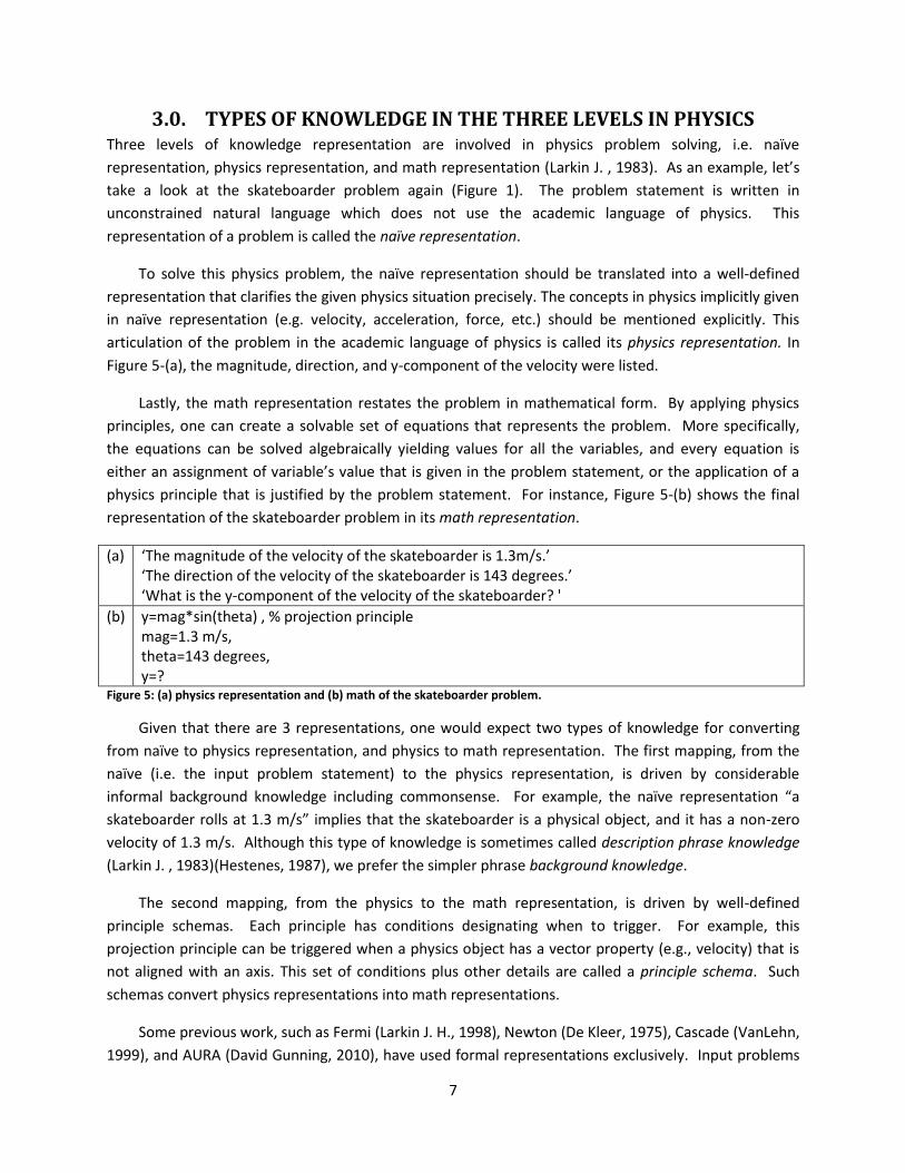
articulation of the problem in the academic language of physics is called its physics representation. In

Figure 5-(a), the magnitude, direction, and y-component of the velocity were listed.

Lastly, the math representation restates the problem in mathematical form. By applying physics

principles, one can create a solvable set of equations that represents the problem. More specifically,

the equations can be solved algebraically yielding values for all the variables, and every equation is

either an assignment of variable’s value that is given in the problem statement, or the application of a

physics principle that is justified by the problem statement. For instance, Figure 5-(b) shows the final

representation of the skateboarder problem in its math representation.

(a) ‘The magnitude of the velocity of the skateboarder is 1.3m/s.’ ‘The direction of the velocity of the skateboarder is 143 degrees.’ ‘What is the y-component of the velocity of the skateboarder? '

(b) y=mag*sin(theta) , % projection principle mag=1.3 m/s, theta=143 degrees, y=?

Figure 5: (a) physics representation and (b) math of the skateboarder problem.

Given that there are 3 representations, one would expect two types of knowledge for converting

from naïve to physics representation, and physics to math representation. The first mapping, from the

naïve (i.e. the input problem statement) to the physics representation, is driven by considerable

informal background knowledge including commonsense. For example, the naïve representation “a

skateboarder rolls at 1.3 m/s” implies that the skateboarder is a physical object, and it has a non-zero

velocity of 1.3 m/s. Although this type of knowledge is sometimes called description phrase knowledge

(Larkin J. , 1983)(Hestenes, 1987), we prefer the simpler phrase background knowledge.

The second mapping, from the physics to the math representation, is driven by well-defined

principle schemas. Each principle has conditions designating when to trigger. For example, this

projection principle can be triggered when a physics object has a vector property (e.g., velocity) that is

not aligned with an axis. This set of conditions plus other details are called a principle schema. Such

schemas convert physics representations into math representations.

Some previous work, such as Fermi (Larkin J. H., 1998), Newton (De Kleer, 1975), Cascade (VanLehn,

1999), and AURA (David Gunning, 2010), have used formal representations exclusively. Input problems

8

were manually translated into formal language versions of a naïve representation. Thus, a partial

formalization of “A skateboarder rolls up an inclined plane” would be physical_object(skateboarder),

surface(plane), supported_by(skateboarder, plane), etc. The physics representation, math

representation, background knowledge and principles schemas were all written in formal language.

Other previous works adopted a method to transform natural language into formal representations

(Mecho (Bundy, Byrd, Luger, Mellish, & Palmer, 1979), ISAAC (Novak Jr., 1977), and pSAT (Ritter,

1998)(Ritter, Anderson, Cytrynowicz, & Medvedeva, 1998)). Their systems were designed to translate

naïve representation in natural language into physics representation in formal language. In this

approach, background knowledge included both domain-specific knowledge (e.g., an inclined plane is a

surface) and natural language processing knowledge. This rather large, diverse knowledgebase was

encoded in program code, and only the system developers were able to change it. So, they still had the

same problem that only the system developers can change background knowledge and the other formal

representations.

The proposed approach in this thesis is to represent both types of knowledge (background

knowledge and principle schemas) in natural language, and to use natural language for the naïve and

the physics representations. The math representation of physics problems will continue to be written in

mathematical notation. In other words, because the naïve representation, background knowledge,

physics representation, and principle schema are all represented in natural language, everything an

author sees from the problem statement onward is in natural language until the very end, when the

mathematical representation is generated by instantiation of generic equations that are part of the

principle schemas. Because authors are assumed to already know math as well as English, they don’t

need to learn new languages or new representations in order to work with the system.

4.0. REPRESENTING KNOWLEDGE IN NATURAL LANGUAGE The problem statement needs to be interpreted so that it can trigger relevant principles. For the

principles to be triggered, the problem must be described in terms of proper scientific concepts such as

forces, accelerations and velocities. Let us define the physics representation more precisely to refer to

the representation that directly matches the principle schemas. Thus, the physics representation of a

problem must use proper scientific concepts such as forces, etc. In theory, the physics representation

could use complex syntax (e.g., relative clauses), pronouns and other constructs of natural language. As

long as a sentence can match rules triggering target principles, the system doesn’t care about the form

of sentences. In this way the system allows authors to write the physics representation in free natural

language. However, authors should write physics representations so that they can trigger relevant

principles with limited matching conditions, so authors will tend to employ a fairly limited range of

linguistic constructs for the physics representations

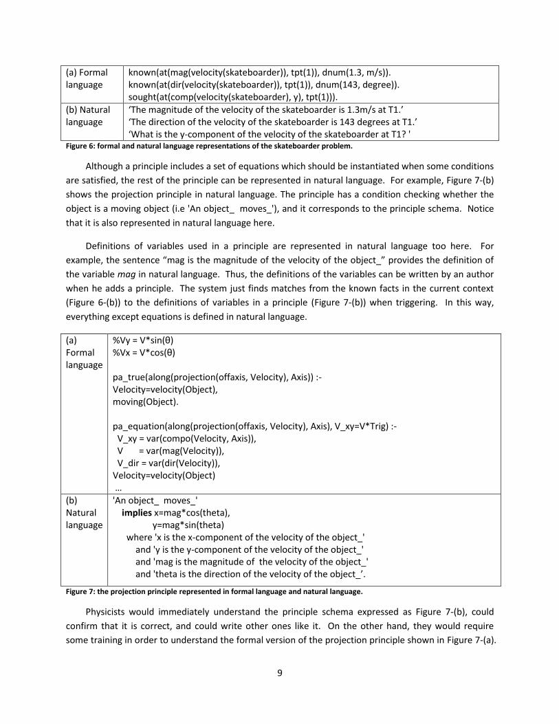
As an example, Figure 6 shows both a formal language and the corresponding natural language

version of the physics representation of the skateboarder problem. It seems plausible that an author

who is trying to debug the translation of a problem could more easily understand physics representation

written in natural language (Figure 6-(b)) rather than formal language (Figure 6-(a)).

9

(a) Formal language

known(at(mag(velocity(skateboarder)), tpt(1)), dnum(1.3, m/s)). known(at(dir(velocity(skateboarder)), tpt(1)), dnum(143, degree)). sought(at(comp(velocity(skateboarder), y), tpt(1))).

(b) Natural language

‘The magnitude of the velocity of the skateboarder is 1.3m/s at T1.’ ‘The direction of the velocity of the skateboarder is 143 degrees at T1.’ ‘What is the y-component of the velocity of the skateboarder at T1? '

Figure 6: formal and natural language representations of the skateboarder problem.

Although a principle includes a set of equations which should be instantiated when some conditions

are satisfied, the rest of the principle can be represented in natural language. For example, Figure 7-(b)

shows the projection principle in natural language. The principle has a condition checking whether the

object is a moving object (i.e 'An object_ moves_'), and it corresponds to the principle schema. Notice

that it is also represented in natural language here.

Definitions of variables used in a principle are represented in natural language too here. For

example, the sentence “mag is the magnitude of the velocity of the object_” provides the definition of

the variable mag in natural language. Thus, the definitions of the variables can be written by an author

when he adds a principle. The system just finds matches from the known facts in the current context

(Figure 6-(b)) to the definitions of variables in a principle (Figure 7-(b)) when triggering. In this way,

everything except equations is defined in natural language.

(a) Formal language

%Vy = V*sin(θ) %Vx = V*cos(θ) pa_true(along(projection(offaxis, Velocity), Axis)) :- Velocity=velocity(Object), moving(Object). pa_equation(along(projection(offaxis, Velocity), Axis), V_xy=V*Trig) :- V_xy = var(compo(Velocity, Axis)), V = var(mag(Velocity)), V_dir = var(dir(Velocity)), Velocity=velocity(Object) …

(b) Natural language

'An object_ moves_' implies x=mag*cos(theta), y=mag*sin(theta) where 'x is the x-component of the velocity of the object_' and 'y is the y-component of the velocity of the object_' and 'mag is the magnitude of the velocity of the object_' and 'theta is the direction of the velocity of the object_’.

Figure 7: the projection principle represented in formal language and natural language.

Physicists would immediately understand the principle schema expressed as Figure 7-(b), could

confirm that it is correct, and could write other ones like it. On the other hand, they would require

some training in order to understand the formal version of the projection principle shown in Figure 7-(a).

10

Even with training, because the formal language will always be relatively less familiar than the natural

language, physicist might overlook minor errors such as misordering of arguments. This formal version

of the principle was from a previous system written in Prolog, so physicists trying to use it would have to

learn the computer language, Prolog in this case. We hypothesize that physics instructors would find it

easier to write, check and debug the natural language versions.

These two figures represent the basic hypothesis. Although the domain mandates that the

conceptual content be translated from naïve to physics to math concepts, it is much easier for authors

to understand this translation if the content is written in natural language rather than a formal language.

4.1. REPRESENTING BACKGROUND KNOWLEDGE The preceding section may suggest that in order to add a new problem to the tutoring system, the

author could write a naïve representation to be read by students, and a physics representation in

natural language to be read by the tutoring system. The physics schemas in the tutoring system would

then translate the given physics representation into a math representation. If that translation failed,

then the author could debug the newly written physics representation and/or the principle schemas

since they are all written in natural language.

While feasible, the approach just sketched is far from optimal. Many researchers have noted

learners make most of their mistakes when translating the naïve representation to the physics

representation. For instance, learners often fail to notice when forces, accelerations, velocities,

displacements and other physics entities are present. Indeed, the background knowledge is often

considered the conceptual core of physics because the principle schemas are important, but not difficult

to learn. Thus, the tutoring system needs to tutor the students as they apply background knowledge.

This means that the tutoring system needs to have a representation of such knowledge. Of course,

some of the background knowledge is familiar (e.g., a skateboarder is a physical object) so it doesn’t

need tutoring.

This motivated developing an intelligent system that can automatically generate physics

representations from a naïve, natural language problem statement. In order to do so, the system should

have background knowledge connecting the problem statement (naïve representation) to the physics

representation. This knowledge includes the description phrase knowledge, and it can include linguistic

knowledge, commonsense knowledge, and domain knowledge from physics. The idea proposed here is

to represent background knowledge in natural language as inference rules, and to let authors add them.

11

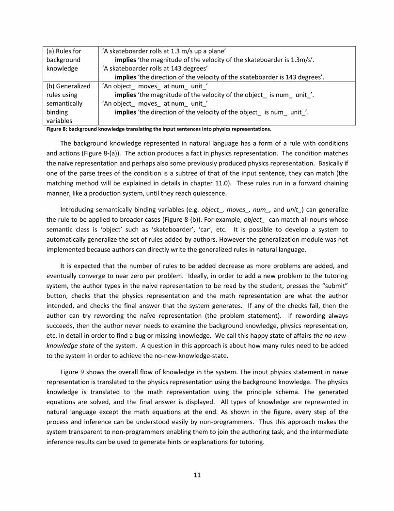
(a) Rules for background knowledge

‘A skateboarder rolls at 1.3 m/s up a plane’ implies ‘the magnitude of the velocity of the skateboarder is 1.3m/s’. ‘A skateboarder rolls at 143 degrees’ implies ‘the direction of the velocity of the skateboarder is 143 degrees’.

(b) Generalized rules using semantically binding variables

‘An object_ moves_ at num_ unit_’ implies ‘the magnitude of the velocity of the object_ is num_ unit_’. ‘An object_ moves_ at num_ unit_’ implies ‘the direction of the velocity of the object_ is num_ unit_’.

Figure 8: background knowledge translating the input sentences into physics representations.

The background knowledge represented in natural language has a form of a rule with conditions

and actions (Figure 8-(a)). The action produces a fact in physics representation. The condition matches

the naïve representation and perhaps also some previously produced physics representation. Basically if

one of the parse trees of the condition is a subtree of that of the input sentence, they can match (the

matching method will be explained in details in chapter 11.0). These rules run in a forward chaining

manner, like a production system, until they reach quiescence.

Introducing semantically binding variables (e.g. object_, moves_, num_, and unit_) can generalize

the rule to be applied to broader cases (Figure 8-(b)). For example, object_ can match all nouns whose

semantic class is ‘object’ such as ‘skateboarder’, ‘car’, etc. It is possible to develop a system to

automatically generalize the set of rules added by authors. However the generalization module was not

implemented because authors can directly write the generalized rules in natural language.

It is expected that the number of rules to be added decrease as more problems are added, and

eventually converge to near zero per problem. Ideally, in order to add a new problem to the tutoring

system, the author types in the naive representation to be read by the student, presses the “submit”

button, checks that the physics representation and the math representation are what the author

intended, and checks the final answer that the system generates. If any of the checks fail, then the

author can try rewording the naïve representation (the problem statement). If rewording always

succeeds, then the author never needs to examine the background knowledge, physics representation,

etc. in detail in order to find a bug or missing knowledge. We call this happy state of affairs the no-new-

knowledge state of the system. A question in this approach is about how many rules need to be added

to the system in order to achieve the no-new-knowledge-state.

Figure 9 shows the overall flow of knowledge in the system. The input physics statement in naïve

representation is translated to the physics representation using the background knowledge. The physics

knowledge is translated to the math representation using the principle schema. The generated

equations are solved, and the final answer is displayed. All types of knowledge are represented in

natural language except the math equations at the end. As shown in the figure, every step of the

process and inference can be understood easily by non-programmers. Thus this approach makes the

system transparent to non-programmers enabling them to join the authoring task, and the intermediate

inference results can be used to generate hints or explanations for tutoring.

12

Figure 9: The five types of knowledge represented in natural language, and their data flow during problem solving.

5.0. SYSTEM ARCHITECTURE OF NATURAL-K Although problems in the physics domain have several types of knowledge, Natural-K, the system

developed here, uses a little different but similar representation for them. Both background knowledge

and principle schema are represented in rules consisting of conditions and actions. Both naïve

representation and physics representation are represented in a natural language sentence. The three

levels of knowledge in physics are processed with one matching engine performing sentence to

sentence matching.

Figure 10 shows the system architecture of Natural-K. The system has mainly three parts - the

matching engine, the knowledgebase, and the context memory. The knowledgebase stores all the

background knowledge written in natural language. Knowledge in natural language is parsed and

Principle Schema:

Background

Knowledge:

‘The object_ moves_' implies y=mag*sin(theta)

where 'y is the y-component of the velocity of the object_'

and 'mag is the magnitude of the velocity of the object_'

and 'theta is the direction of the velocity of the object_’.

Naïve

Representation:

Physics

Representation:

Math

Representation:

y=mag*sin(theta) , mag=1.3 m/s, theta=143 degrees,

y=?

‘A skateboarder rolls at 1.3 m/s up a plane’ implies ‘the

magnitude of the velocity of the skateboarder is 1.3m/s’.

…

“A skateboarder rolls at 1.3 m/s up an inclined plane angled at

143 degrees. What is its vertical velocity?”

‘The magnitude of the velocity of the skateboarder is 1.3 m/s.’

‘The direction of the velocity of the skateboarder is 143 degrees.’

‘What is the y-component of the velocity of the skateboarder? '

y = 0.78 m/s

The y-component of the velocity of the skateboarder is 0.78 m/s

Answer:

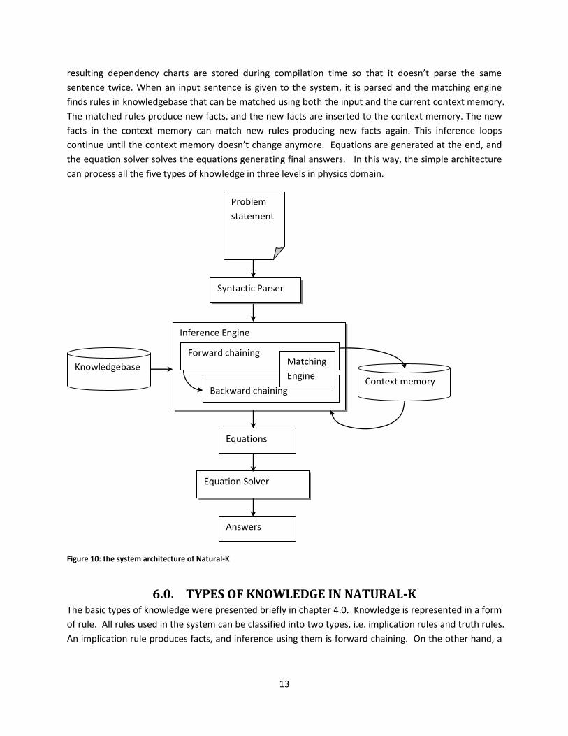
13

resulting dependency charts are stored during compilation time so that it doesn’t parse the same

sentence twice. When an input sentence is given to the system, it is parsed and the matching engine

finds rules in knowledgebase that can be matched using both the input and the current context memory.

The matched rules produce new facts, and the new facts are inserted to the context memory. The new

facts in the context memory can match new rules producing new facts again. This inference loops

continue until the context memory doesn’t change anymore. Equations are generated at the end, and

the equation solver solves the equations generating final answers. In this way, the simple architecture

can process all the five types of knowledge in three levels in physics domain.

Figure 10: the system architecture of Natural-K

6.0. TYPES OF KNOWLEDGE IN NATURAL-K The basic types of knowledge were presented briefly in chapter 4.0. Knowledge is represented in a form

of rule. All rules used in the system can be classified into two types, i.e. implication rules and truth rules.

An implication rule produces facts, and inference using them is forward chaining. On the other hand, a

Inference Engine

Backward chaining

Forward chaining Matching

Engine

Knowledgebase

Problem

statement

Syntactic Parser

Equations

Equation Solver

Answers

Context memory

14

truth rule only checks truth, and does not produce any fact. Inference using truth rules is backward

chaining.

Implication rules include default rules, negation rules, and principles. Truth rules include logic rules

and math rules. Their representation using natural language is presented in this chapter in detail.

6.1. IMPLICATION RULES A background rule has conditions in the left side and actions in the right side. Input sentences and

known facts match conditions. If all the conditions are satisfied, the actions in the right side are

generated as facts. The generated facts are used to trigger other rules. Multiple conditions (and actions)

are connected with ‘and’ connector. Each condition and action is a natural language sentence enclosed

with quotation marks (‘…’).

<condition 1> and <condition 2> and … <condition N> imply <action 1> and <action 2> … and <action N>. Figure 11: the basic form of an implication rule

6.1.1. Default Rule

Some facts are naturally assumed by default. When a physics problem describes a situation about a ball

thrown, it is assumed that the ball is thrown nearby the earth if there is no mention about a nearby

planet. Let’s call such knowledge default knowledge, and a rule for default knowledge a default rule. A

condition of the default rule has a tag unknown notifying that the condition is satisfied only when there

is no fact that can match.

‘The location is near a planet_’ unknown implies ‘the location is near the earth‘. 'The location is near the earth' and 'the magnitude of the gravitational acceleration on the earth is num_ unit_' unknown imply 'the magnitude of the gravitational acceleration on the earth is 9.8 m/s^2'. Figure 12: examples of default rules

One of the important properties of natural language is that background knowledge has a major role

in inference. A default rule also works as background knowledge, and it is triggered based on unknown

facts. Often only some of conditions are satisfied by default, and it is possible that the default rule has

both known and unknown conditions. Figure 12 shows two default rules. In the first one, the fact ‘the

location is near the earth’ is generated by default when there is no mention about a nearby planet. In

the second one, the fact about the gravitational acceleration 9.8 m/s^2 is generated when it is not

mentioned and the location is near the earth.

15

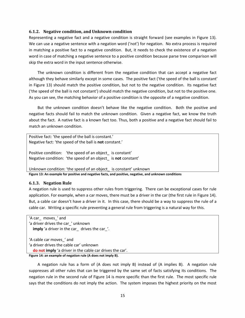
6.1.2. Negative condition, and Unknown condition

Representing a negative fact and a negative condition is straight forward (see examples in Figure 13).

We can use a negative sentence with a negation word (‘not’) for negation. No extra process is required

in matching a positive fact to a negative condition. But, it needs to check the existence of a negation

word in case of matching a negative sentence to a positive condition because parse tree comparison will

skip the extra word in the input sentence otherwise.

The unknown condition is different from the negative condition that can accept a negative fact

although they behave similarly except in some cases. The positive fact (‘the speed of the ball is constant’

in Figure 13) should match the positive condition, but not to the negative condition. Its negative fact

(‘the speed of the ball is not constant’) should match the negative condition, but not to the positive one.

As you can see, the matching behavior of a positive condition is the opposite of a negative condition.

But the unknown condition doesn’t behave like the negative condition. Both the positive and

negative facts should fail to match the unknown condition. Given a negative fact, we know the truth

about the fact. A native fact is a known fact too. Thus, both a positive and a negative fact should fail to

match an unknown condition.

Positive fact: ‘the speed of the ball is constant.’ Negative fact: ‘the speed of the ball is not constant.’ Positive condition: ‘the speed of an object_ is constant’ Negative condition: ‘the speed of an object_ is not constant’ Unknown condition: ‘the speed of an object_ is constant’ unknown Figure 13: An example for positive and negative facts, and positive, negative, and unknown conditions

6.1.3. Negation Rule

A negation rule is used to suppress other rules from triggering. There can be exceptional cases for rule

application. For example, when a car moves, there must be a driver in the car (the first rule in Figure 14).

But, a cable car doesn’t have a driver in it. In this case, there should be a way to suppress the rule of a

cable car. Writing a specific rule preventing a general rule from triggering is a natural way for this.

‘A car_ moves_' and ‘a driver drives the car_' unknown imply 'a driver in the car_ drives the car_‘. ‘A cable car moves_‘ and ‘a driver drives the cable car’ unknown do not imply ‘a driver in the cable car drives the car'. Figure 14: an example of negation rule (A does not imply B).

A negation rule has a form of (A does not imply B) instead of (A implies B). A negation rule

suppresses all other rules that can be triggered by the same set of facts satisfying its conditions. The

negation rule in the second rule of Figure 14 is more specific than the first rule. The most specific rule

says that the conditions do not imply the action. The system imposes the highest priority on the most

16

specific rule matched. Thus the more general rule (the first rule) is not triggered. The subsumption

relation between two rules is used to find the most specific rule, and it will be explained in the inference

section (chapter 10.3).

A negation rule can be used to deal with over-generation problems. It is enough to add a more

specific negation rule if a user finds a fact that is not supposed to be generated. He can check the

background rules generating the fact, and write a negation rule for the specific case to suppress it.

6.1.4. Principles

One of the significant ideas proposed in this thesis is that principles can be represented in natural

language too. As shown in Figure 7-(a), principles were encoded in program codes in the previous

approaches, and it was the reason why only programmers were able to update principles. By

representing principles in natural language, non-programmers are enabled to update principles too.

A principle rule is a kind of implication rule. The same matching module is used for principle rules

and other implication rules. The only difference is that the output of a principle rule is equations. The

basic form of a principle is almost the same as that of an implication rule (Figure 11) except the ‘where’

phrase at the end. The definitions of variables in the equations are given to the ‘where‘ phrase. An

example of a principle is given in Figure 7-(b).

<condition 1> and <condition 2> and … <condition N> imply <equations> where <variable definition 1> and <variable definition 2> … and <variable definition N>. Figure 15: the basic form of a principle

6.2. TRUTH RULES Input sentences trigger implication rules producing new facts. Implication rules are used for forward

chaining producing new facts. Truth rules work the opposite way. Truth Rules don’t produce anything

only checking truth of hypothesis. A truth rule has hypotheses in the left side and conditions in the right

side (Figure 16). If all the conditions are satisfied, then all the hypotheses become true.

<hypothesis 1> and < hypothesis 2> and … < hypothesis N> if <condition 1> and <condition 2> … and <condition N>. Figure 16: the basic from of a truth rule

17

It is true that an object moves at the interval between T1 and T3 if it moves between T1 and T2 and

between T2 and T3. This logic was represented by the first rule in Figure 17. The second truth rule can

be used to check the truth of facts in sub intervals. If an object moves between T1 and T3, then it is true

that it moves between T1 and T2, and between T2 and T3.

'An object_ moves_ at the interval between Ti_ and Tk_' if 'the object_ moves_ at the interval between Ti_ and Tj_' and 'the object_ moves_ at the interval between Tj_ and Tk_'. 'An object_ moves_ at the interval between Ti_ and Tj_' and 'the object_ moves_ at the interval between Tj_ and Tk_' if 'the object_ moves_ at the interval between Ti_ and Tk_'. Figure 17: examples of truth rule

During inference, the system tries to find an existing fact in the context memory to match a

condition in an implication rule. When there is no such fact, it tries to validate the condition from truth

rules. First, it finds the matching hypothesis in a truth rule. Second, it checks validity of the conditions in

the truth rules. Some of the conditions can be matched by existing facts. The other conditions failing to

match by existing facts can match other truth rules. This chain of inference is backward chaining

starting from hypothesis searching toward existing facts.

The truth rules can be used to find an answer for a qualitative question. For example, ‘does the ball

go higher than 3 m?’ requires comparing the height of the ball at the apex and 3 m. Figure 18 shows

truth rules to validate this question. The input question matches the hypothesis of the rule, and if all the

conditions in the right side are satisfied by existing facts, then the hypothesis becomes true. As you can

see, representing knowledge for a qualitative question can be naturally done, and it is one of the

advantages of using natural language as knowledge representation.

Input: ‘Does the ball go higher than 3 m?’

Rule: ‘An object_ goes higher than num1_ unit_’ If ‘the maximum height of the object_ is num2_ unit_’ and ‘num2_ is larger than num1_’. ‘The maximum height of an object_ is num_ unit_’ If ‘the magnitude of the displacement of the object_ is num_ unit_ at the interval between Ti_ and Tj_’ and ‘the object_ starts to move at Ti_’ and ‘the object_ is at the apex at Tj_’. Figure 18: a qualitative question and a truth rule to check the validity

Truth rules are useful in reducing the number of produced facts. After a truth rule is triggered, the

verified hypotheses are not generated as facts, and they don’t trigger other rules. It can be useful to

reduce the number of facts generated during inference. An author can choose between truth rules and

18

implication rules to represent knowledge though truth rules are mainly used for logic and math. It will

be explained in details later when explaining backward chaining (chapter 10.1).

6.2.1. Logic Rule Truth rules are used for simple logic and math processing. The condition (the right side) of a rule is logic

(or math) expression, and the system has a predefined module to process the logic expression. Figure

19 shows examples of logic and math rules. Note that the conditions in the right side of the rules are

not string. The first example is for numeric comparison of two numbers. The second one is for

summation of two numbers. Mid time point creation is also done by logic rules. The third example is

for mid time point creation. Even though the right side of the rule allows only predefined expressions,

corresponding natural language expression in the left side is not limited, and implication rules can be

added to accept paraphrases.

'num1_ is smaller than num2_' if num1_ < num2_. 'num3_ is num1_ + num2_' if num3_ = num1_ + num2_. ‘Tj_ is a time point between Ti_ and Tk_’ If Tj_= mid(Ti_, Tk_). Figure 19: examples of truth rule for logic and math

Let’s assume that the input “a swimmer reaches a place which is 35 deg west of north” is given

(Figure 20), and the system should infer that the actual direction of the swimmer is 35+90 degrees. The

condition ‘num2_ is num_ + 90’ is required in the truth rule to calculate it (the second condition of the

rule in Figure 20). The value 35 will match num_ in the first condition of the rule. The second condition

of the rule will match the hypothesis of the math rule (the second rule) in Figure 19. The value 90 will

match num2_ in the math rule. The math rule will assign 125 to num3_ after calculation, and this value

will be assigned to num2_ in the second condition of the rule in Figure 20. The condition is satisfied and

the action part of the rule will be generated as a fact (i.e. ‘the direction of the displacement of the

swimmer is 125 degrees’).

Input: 'A swimmer reaches a place which is 35 deg west of north.‘

Rule: ‘An object_ reaches_ a place_ which is num_ unitAngle_ west of north' and 'num2_ is num_ + 90' imply 'the direction of the displacement of the object_ is num2_ unitAngle_'. Figure 20: an example sentence and a truth rule for math to calculate the actual direction (35+90 degrees)

7.0. GENERALIZED REPRESENTATION Unrestricted natural language is allowed in conditions, actions, and hypotheses of a rule. As long as two

sentences match, the form of the sentences doesn’t matter. Theoretically ungrammatical sentences

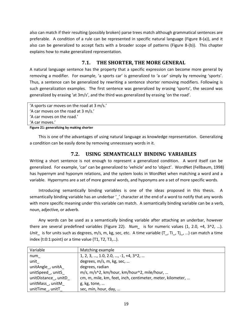
19

also can match if their resulting (possibly broken) parse trees match although grammatical sentences are

preferable. A condition of a rule can be represented in specific natural language (Figure 8-(a)), and it

also can be generalized to accept facts with a broader scope of patterns (Figure 8-(b)). This chapter

explains how to make generalized representation.

7.1. THE SHORTER, THE MORE GENERAL A natural language sentence has the property that a specific expression can become more general by

removing a modifier. For example, ‘a sports car’ is generalized to ‘a car’ simply by removing ‘sports’.

Thus, a sentence can be generalized by rewriting a sentence shorter removing modifiers. Following is

such generalization examples. The first sentence was generalized by erasing ‘sports’, the second was

generalized by erasing ‘at 3m/s’, and the third was generalized by erasing ‘on the road’.

‘A sports car moves on the road at 3 m/s.’ ‘A car moves on the road at 3 m/s.’ ‘A car moves on the road.’ ‘A car moves.’ Figure 21: generalizing by making shorter

This is one of the advantages of using natural language as knowledge representation. Generalizing

a condition can be easily done by removing unnecessary words in it.

7.2. USING SEMANTICALLY BINDING VARIABLES Writing a short sentence is not enough to represent a generalized condition. A word itself can be

generalized. For example, ‘car’ can be generalized to ‘vehicle’ and to ‘object’. WordNet (Fellbaum, 1998)

has hypernym and hyponym relations, and the system looks in WordNet when matching a word and a

variable. Hypernyms are a set of more general words, and hyponyms are a set of more specific words.

Introducing semantically binding variables is one of the ideas proposed in this thesis. A

semantically binding variable has an underbar ‘_’ character at the end of a word to notify that any words

with more specific meaning under this variable can match. A semantically binding variable can be a verb,

noun, adjective, or adverb.

Any words can be used as a semantically binding variable after attaching an underbar, however

there are several predefined variables (Figure 22). Num_ is for numeric values (1, 2.0, +4, 3^2, …).

Unit_ is for units such as degrees, m/s, m, kg, sec, etc. A time variable (T_, Ti_, Tj_, …) can match a time

index (t:0:1:point) or a time value (T1, T2, T3,…).

Variable Matching example

num_ unit_ unitAngle_, unitA_ unitSpeed_, unitS_ unitDistance_, unitD_ unitMass_, unitM_ unitTime_, unitT_

1, 2, 3, …, 1.0, 2.0, …, -1, +4, 3^2, … degrees, m/s, m, kg, sec, … degrees, radian m/s, m/s^2, km/hour, km/hour^2, mile/hour, … cm, m, mile, km, feet, inch, centimeter, meter, kilometer, … g, kg, tone, … sec, min, hour, day, …

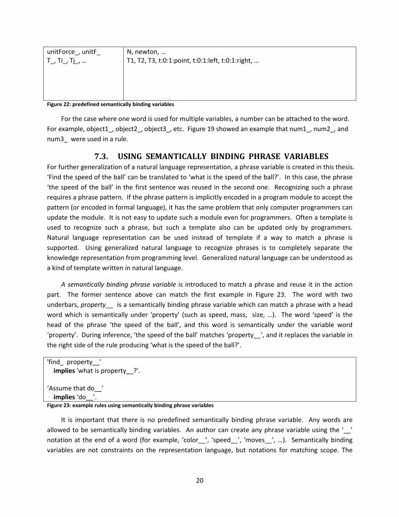
20

unitForce_, unitF_ T_, Ti_, Tj_, …

N, newton, … T1, T2, T3, t:0:1:point, t:0:1:left, t:0:1:right, …

Figure 22: predefined semantically binding variables

For the case where one word is used for multiple variables, a number can be attached to the word.

For example, object1_, object2_, object3_, etc. Figure 19 showed an example that num1_, num2_, and

num3_ were used in a rule.

7.3. USING SEMANTICALLY BINDING PHRASE VARIABLES For further generalization of a natural language representation, a phrase variable is created in this thesis.

‘Find the speed of the ball’ can be translated to ‘what is the speed of the ball?’. In this case, the phrase

‘the speed of the ball’ in the first sentence was reused in the second one. Recognizing such a phrase

requires a phrase pattern. If the phrase pattern is implicitly encoded in a program module to accept the

pattern (or encoded in formal language), it has the same problem that only computer programmers can

update the module. It is not easy to update such a module even for programmers. Often a template is

used to recognize such a phrase, but such a template also can be updated only by programmers.

Natural language representation can be used instead of template if a way to match a phrase is

supported. Using generalized natural language to recognize phrases is to completely separate the

knowledge representation from programming level. Generalized natural language can be understood as

a kind of template written in natural language.

A semantically binding phrase variable is introduced to match a phrase and reuse it in the action

part. The former sentence above can match the first example in Figure 23. The word with two

underbars, property__ is a semantically binding phrase variable which can match a phrase with a head

word which is semantically under ‘property’ (such as speed, mass, size, …). The word ‘speed’ is the

head of the phrase ‘the speed of the ball’, and this word is semantically under the variable word

‘property’. During inference, ‘the speed of the ball’ matches ‘property__’, and it replaces the variable in

the right side of the rule producing ‘what is the speed of the ball?’.

'find_ property__' implies 'what is property__?'. ‘Assume that do__’ implies ‘do__’. Figure 23: example rules using semantically binding phrase variables

It is important that there is no predefined semantically binding phrase variable. Any words are

allowed to be semantically binding variables. An author can create any phrase variable using the ‘__’

notation at the end of a word (for example, ‘color__’, ‘speed__’, ‘moves__’, …). Semantically binding

variables are not constraints on the representation language, but notations for matching scope. The

21

system looks in WordNet when matching a semantically binding variable and the head word of an input

phrase.

A phrase variable can match a clause too. An input ‘assume that the car moves in a constant speed’

can match the condition of the second rule in Figure 23. The head word of the clause is ‘moves’, and it

matches the phrase variable ‘do__’ which can match any active verb. Thus the clause ‘the car moves in

a constant speed’ matches ‘do__’, and the action of the rule becomes ‘the car moves in a constant

speed’.

A phrase variable has a significant role in time phrase processing such as ‘when …’ and ‘after …’. It

will be explained in the time phrase section (chapter 8.3) in detail.

8.0. REPRESENTING TIME English often does not represent time explicitly, but the physics representation must represent time

explicitly. So, some background rules are needed to handle this explication. The rule interpretation

mechanisms described so far were not enough for this, so additional mechanisms had to be invented,

and they will be described in this chapter. Basically, there should be a way to create a time point, a way

to refer to an existing time point in the natural language framework. The rules are quite general, so

once an initial author (such as a knowledge engineer) who understands these new mechanisms has

written the appropriate rules, a subsequent author (e.g. an instructor or student) doesn't need to write

any more time rules.

Physics events occurring in a physics world can be ordered in time sequence. An event can occur

before (or after) another event, or they can occur at the same time. For example, a human can naturally

understand that the event of a ball thrown upward is followed by the event of the ball hitting the

ground. This time relation is represented by time variables such as T1, T2, …, Tn in physics textbook.

The magnitude of the velocity of the ball is 16.0 m/s at T1 Figure 24: a fact with a time point

However, a problem statement (or native representation) usually doesn’t have any time point

because students are supposed to understand the problem and build a corresponding physics mental

model to solve. Thus, an event in a naïve representation should be translated to a physics

representation with a time point.

Throwing upward: ‘A ball is thrown vertically upward with a speed of 16.0 m/s. How long is the ball in the air?’

Figure 25: Problem statement of throwing upward

Also, there needs to be a representation to create a new time point. It is done by a new time

variable in the right side of a rule. If there is a new time variable in the right side, then a new time point

is assigned to the variable. A time variable for a time point starts with ‘T’ and ends with ‘_’ like a

semantically binding variable. In the first example of Figure 26, the time variable ‘T_’ doesn’t appear in

the left side of the rule, so a new time point is assigned to it. However, in the second example, the time

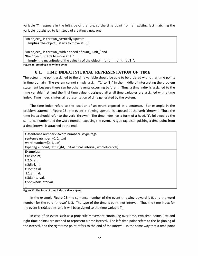
22

variable ‘T_’ appears in the left side of the rule, so the time point from an existing fact matching the

variable is assigned to it instead of creating a new one.

‘An object_ is thrown_ vertically upward’ Implies ‘the object_ starts to move at T_’. ‘An object_ is thrown_ with a speed of num_ unit_’ and ‘the object_ starts to move at T_’ Imply ‘the magnitude of the velocity of the object_ is num_ unit_ at T_’.

Figure 26: creating a new time point

8.1. TIME INDEX: INTERNAL REPRESENTATION OF TIME The actual time point assigned to the time variable should be able to be ordered with other time points

in time domain. The system cannot simply assign ‘T1’ to ‘T_’ in the middle of interpreting the problem

statement because there can be other events occurring before it. Thus, a time index is assigned to the

time variable first, and the final time value is assigned after all time variables are assigned with a time

index. Time index is internal representation of time generated by the system.

The time index refers to the location of an event exposed in a sentence. For example in the

problem statement Figure 25 , the event ‘throwing upward’ is exposed at the verb ‘thrown’. Thus, the

time index should refer to the verb ‘thrown’. The time index has a form of a head, ‘t’, followed by the

sentence number and the word number exposing the event. A type tag distinguishing a time point from

a time interval is attached at the end.

t:<sentence number>:<word number>:<type tag> sentence number={0, 1, …n} word number={0, 1, …n} type tag = {point, left, right, initial, final, interval, wholeInterval}

Examples: t:0:3:point, t:2:5:left, t:2:5:right, t:1:2:initial, t:1:2:final, t:3:3:interval, t:5:2:wholeInterval, …

Figure 27: The form of time index and examples.

In the example Figure 25, the sentence number of the event throwing upward is 0, and the word

number for the verb ‘thrown’ is 3. The type of the time is point, not interval. Thus the time index for

the event is t:0:3:point, and it will be assigned to the time variable T_.

In case of an event such as a projectile movement continuing over time, two time points (left and

right time points) are needed to represent a time interval. The left time point refers to the beginning of

the interval, and the right time point refers to the end of the interval. In the same way that a time point

23

is created, a time interval can be created by creating the two time points. The time variable for a left

time point is ‘Ti_’, and for a right time point is ‘Tj_’. In Figure 28, the two time variables were used only

in the right side of the rule, so a new time index is assigned to each time variable. If the problem

statement of throwing upward (Figure 25) matches this rule, t:0:3:left will be assigned to Ti_, and

t:0:3:right will be assigned to Tj_.

‘An object_ is thrown_’ Implies ‘the object_ moves at the interval between Ti_ and Tj_’. Figure 28: creating a new time interval

The resulting facts generated so far are as following:

‘the ball starts to move at t:0:3:point.’ ‘the magnitude of the velocity of the ball is 3 m/s at t:0:3:point.’ ‘the ball moves at the interval between t:0:3:left and t:0:3:right.’ Figure 29: generated facts with a time index assigned

This method creating a time index referring to a verb in a sentence allows to assign multiple time

points when more than one event is described in a problem statement. For example, there are two

physics events in Figure 30. The one is the ball’s throwing upward, and the other is the bug’s freefall.

The background rule in Figure 28 and a corresponding rule for freefall (not shown here) will match the

two input sentences creating two time intervals. One time index will be assigned to the point of the

verb ‘thrown’ in the first sentence, and another time index will be assigned to point of the verb ‘free-fall’

in the second sentence. In this way, the system can recognize that the first event occurs before the

second event.

A Startled Bug: ‘A ball was thrown straight upward at 3 m/s inside a building. The ball hits the ceiling one second later, and a startled bug on the ceiling starts to free-fall. How long does it take for the bug to hit the floor?’ Figure 30: an example with two time intervals

In most cases, a time index can be assigned to a generated fact when a background rule with a new

time variable is triggered. But, there are cases that a time index should be assigned based on a word in

a sentence. Some sentence expresses a type of time in an adjective. For example, ‘the initial velocity of

the ball is 3 m/s’ provides a value of the initial velocity, and the adjective ‘initial’ has a role to determine

the type of the time. In this case, a time index of initial type is assigned to the fact, and the final time

value for it is assigned after all time points are generated. In the similar way, a time index of ‘interval’

type is assigned to a fact describing an event with a time interval. It will be explained in details in the

chapter 8.3.

In many physics problems, it is required to represent an event occurring between two events. For

example, the event of an object reaching the apex of projectile occurs between the event throwing

upward and the event hitting the ground. The internal representation of time in the middle of two time

points is t:mid(Ti_, Tk_). It will be explained in mental model extension again (chapter 0).

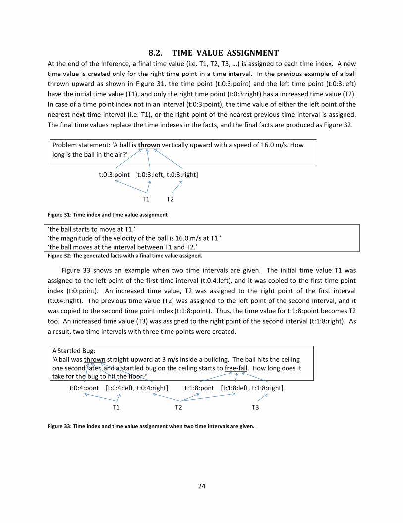
24

8.2. TIME VALUE ASSIGNMENT At the end of the inference, a final time value (i.e. T1, T2, T3, …) is assigned to each time index. A new

time value is created only for the right time point in a time interval. In the previous example of a ball

thrown upward as shown in Figure 31, the time point (t:0:3:point) and the left time point (t:0:3:left)

have the initial time value (T1), and only the right time point (t:0:3:right) has a increased time value (T2).

In case of a time point index not in an interval (t:0:3:point), the time value of either the left point of the

nearest next time interval (i.e. T1), or the right point of the nearest previous time interval is assigned.

The final time values replace the time indexes in the facts, and the final facts are produced as Figure 32.

Problem statement: 'A ball is thrown vertically upward with a speed of 16.0 m/s. How

long is the ball in the air?'

t:0:3:point [t:0:3:left, t:0:3:right]

T1 T2

Figure 31: Time index and time value assignment

‘the ball starts to move at T1.’ ‘the magnitude of the velocity of the ball is 16.0 m/s at T1.’ ‘the ball moves at the interval between T1 and T2.’ Figure 32: The generated facts with a final time value assigned.

Figure 33 shows an example when two time intervals are given. The initial time value T1 was

assigned to the left point of the first time interval (t:0:4:left), and it was copied to the first time point

index (t:0:point). An increased time value, T2 was assigned to the right point of the first interval

(t:0:4:right). The previous time value (T2) was assigned to the left point of the second interval, and it

was copied to the second time point index (t:1:8:point). Thus, the time value for t:1:8:point becomes T2

too. An increased time value (T3) was assigned to the right point of the second interval (t:1:8:right). As

a result, two time intervals with three time points were created.

A Startled Bug:‘A ball was thrown straight upward at 3 m/s inside a building. The ball hits the ceiling one second later, and a startled bug on the ceiling starts to free-fall. How long does it take for the bug to hit the floor?’

t:0:4:pont [t:0:4:left, t:0:4:right]

T1 T2

t:1:8:pont [t:1:8:left, t:1:8:right]

T3

Figure 33: Time index and time value assignment when two time intervals are given.

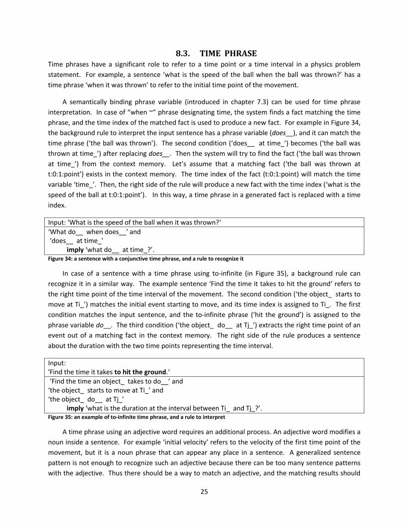
25

8.3. TIME PHRASE Time phrases have a significant role to refer to a time point or a time interval in a physics problem

statement. For example, a sentence ‘what is the speed of the ball when the ball was thrown?’ has a

time phrase ‘when it was thrown’ to refer to the initial time point of the movement.

A semantically binding phrase variable (introduced in chapter 7.3) can be used for time phrase

interpretation. In case of “when ~” phrase designating time, the system finds a fact matching the time

phrase, and the time index of the matched fact is used to produce a new fact. For example in Figure 34,

the background rule to interpret the input sentence has a phrase variable (does__), and it can match the

time phrase (‘the ball was thrown’). The second condition (‘does__ at time_’) becomes (‘the ball was

thrown at time_’) after replacing does__. Then the system will try to find the fact (‘the ball was thrown

at time_’) from the context memory. Let’s assume that a matching fact (‘the ball was thrown at

t:0:1:point’) exists in the context memory. The time index of the fact (t:0:1:point) will match the time

variable ‘time_’. Then, the right side of the rule will produce a new fact with the time index (‘what is the

speed of the ball at t:0:1:point’). In this way, a time phrase in a generated fact is replaced with a time

index.

Input: 'What is the speed of the ball when it was thrown?‘

‘What do__ when does__’ and ‘does__ at time_’

imply ‘what do__ at time_?’. Figure 34: a sentence with a conjunctive time phrase, and a rule to recognize it

In case of a sentence with a time phrase using to-infinite (in Figure 35), a background rule can

recognize it in a similar way. The example sentence ‘Find the time it takes to hit the ground‘ refers to

the right time point of the time interval of the movement. The second condition (‘the object_ starts to

move at Ti_’) matches the initial event starting to move, and its time index is assigned to Ti_. The first

condition matches the input sentence, and the to-infinite phrase (‘hit the ground’) is assigned to the

phrase variable do__. The third condition (‘the object_ do__ at Tj_’) extracts the right time point of an

event out of a matching fact in the context memory. The right side of the rule produces a sentence

about the duration with the two time points representing the time interval.

Input: 'Find the time it takes to hit the ground.‘

‘Find the time an object_ takes to do__’ and ‘the object_ starts to move at Ti_’ and ‘the object_ do__ at Tj_’

imply ‘what is the duration at the interval between Ti_ and Tj_?’. Figure 35: an example of to-infinite time phrase, and a rule to interpret

A time phrase using an adjective word requires an additional process. An adjective word modifies a

noun inside a sentence. For example ‘initial velocity’ refers to the velocity of the first time point of the

movement, but it is a noun phrase that can appear any place in a sentence. A generalized sentence

pattern is not enough to recognize such an adjective because there can be too many sentence patterns

with the adjective. Thus there should be a way to match an adjective, and the matching results should

26

be passed to the time value of the sentence. The first rule in Figure 36 accepts a sentence describing the

value of a vector. The phrase variable ‘vector__’ will match the adjective time phrase ‘the initial

velocity’. Then the system tries to find other rules that can match the phrase. The phrase will match the

second rule generating the initial time tag time(initial), and it will be passed up to the sentence assigning

initial time point (for example, t:0:6:initial). In this way, a part of an input sentence matching a phrase

variable can trigger other rules, and it is used to recognize adjective time phrase.

Input: ‘The initial velocity of the ball is 3 m/s.‘

‘vector__ is num_ unitS_’ implies ‘the magnitude of the vector__ is num_ unitS_’.

‘initial vector_’ implies time(initial).

Figure 36: an example of adjective time phrase (initial~, final~, whole~, total~), and rules to interpret

There are more types of time phrases using a preposition, and a relative clause. They can be

recognized using background rules as Figure 37. Also, quantities other than time can be represented

using a phrase. The magnitude of the displacement zero was represented using a prepositional phrase in

Figure 37-(3).

1. Relative clause Ex) 'What is the total time for which the ball remains in air?' Rule) ‘what is something_ for which do__?’ and ‘do__ at time_interval_’ implies ‘what is something_ at time_interval_?’.

2. Prepositional time Ex) 'What is the ball's speed at the end of 5 seconds?’

Rule) ‘What is the object_'s speed at the end of num_ unitT_?’and ‘the object_ starts to move at Ti_’ and ‘the duration is num_ unitT_ at the interval between Ti_ and Tj_’ imply ‘what is the speed of the object_ at Tj_?’. 3. Etc. other quantities can be referred using a phrase

Ex) ‘The ball is caught at the same height from which it was released.’ Rule) ‘An object_ does__ at the same height from which it was released’ and ‘the object_ returns to the initial level at T_’ implies ‘the object_ does__ at T_’. Figure 37: types of time phrases, and corresponding rules to interpret them

In this way, time was represented in a natural language framework. The introduced representation

using time variables (Ti_, Tj_, …) and time phrases (‘when does__’) are general enough to be reused so

that they don’t need to be added again once added.

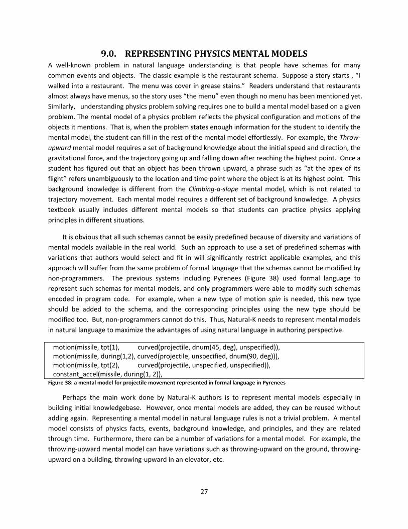
27

9.0. REPRESENTING PHYSICS MENTAL MODELS A well-known problem in natural language understanding is that people have schemas for many

common events and objects. The classic example is the restaurant schema. Suppose a story starts , “I

walked into a restaurant. The menu was cover in grease stains.” Readers understand that restaurants

almost always have menus, so the story uses “the menu” even though no menu has been mentioned yet.

Similarly, understanding physics problem solving requires one to build a mental model based on a given

problem. The mental model of a physics problem reflects the physical configuration and motions of the

objects it mentions. That is, when the problem states enough information for the student to identify the

mental model, the student can fill in the rest of the mental model effortlessly. For example, the Throw-

upward mental model requires a set of background knowledge about the initial speed and direction, the

gravitational force, and the trajectory going up and falling down after reaching the highest point. Once a

student has figured out that an object has been thrown upward, a phrase such as “at the apex of its

flight” refers unambiguously to the location and time point where the object is at its highest point. This

background knowledge is different from the Climbing-a-slope mental model, which is not related to

trajectory movement. Each mental model requires a different set of background knowledge. A physics

textbook usually includes different mental models so that students can practice physics applying

principles in different situations.

It is obvious that all such schemas cannot be easily predefined because of diversity and variations of

mental models available in the real world. Such an approach to use a set of predefined schemas with

variations that authors would select and fit in will significantly restrict applicable examples, and this

approach will suffer from the same problem of formal language that the schemas cannot be modified by

non-programmers. The previous systems including Pyrenees (Figure 38) used formal language to

represent such schemas for mental models, and only programmers were able to modify such schemas

encoded in program code. For example, when a new type of motion spin is needed, this new type

should be added to the schema, and the corresponding principles using the new type should be

modified too. But, non-programmers cannot do this. Thus, Natural-K needs to represent mental models

in natural language to maximize the advantages of using natural language in authoring perspective.

motion(missile, tpt(1), curved(projectile, dnum(45, deg), unspecified)), motion(missile, during(1,2), curved(projectile, unspecified, dnum(90, deg))), motion(missile, tpt(2), curved(projectile, unspecified, unspecified)), constant_accel(missile, during(1, 2)), Figure 38: a mental model for projectile movement represented in formal language in Pyrenees

Perhaps the main work done by Natural-K authors is to represent mental models especially in

building initial knowledgebase. However, once mental models are added, they can be reused without

adding again. Representing a mental model in natural language rules is not a trivial problem. A mental

model consists of physics facts, events, background knowledge, and principles, and they are related

through time. Furthermore, there can be a number of variations for a mental model. For example, the

throwing-upward mental model can have variations such as throwing-upward on the ground, throwing-

upward on a building, throwing-upward in an elevator, etc.

28

As an illustration of the kind of work that a Natural-K author must do, this chapter discusses a

physics mental model and its various extensions. The throwing-upward mental model will be used

through this chapter. As discussed later, many mental models have been represented in Natural-K.

Doing this authoring required no new representational mechanisms beyond those presented already,

namely: rules, principles, semantically binding words and time phrases, and temporal reasoning.

9.1. A BASIC MENTAL MODEL A basic mental model has basic knowledge for physics events. In case of an object thrown upward, this

event can be modeled by the starting movement, the ending movement, and the movement between

the two events as shown in Figure 39.

Ti Tj

'the object_ starts to move straight up at Ti_.‘ 'the object_ hits the ground at Tj_.‘

Figure 39: the basic mental model for throwing upward

The starting movement of an object at a time point is represented by ‘the object_ starts to move

straight up at T_’. This is a natural language sentence with semantically binding variables (object_, and

T_). This representation is given to a right side of a background rule to produce an event of the starting

movement. This rule should be triggered when a problem statement includes a sentence matching ‘an

object_ is thrown_ upward_’, and this representation is given to the condition of the rule. The variable

T_ appears only at the right side of the rule, so a time index referring to a time point will be created (for

example, t:0:3:point).

'An object_ is thrown_ upward_‘ implies 'the object_ starts to move straight up at T_‘. Figure 40: a rule for starting movement

The second rule describes the movement of the object at a time interval, and the ending movement.

The movement of the object in the time interval is represented by ‘the object_ moves at the interval

between Ti_ and Tj_’. The ending of the movement is represented by ‘the object_ hits the ground at

Tj_’. This rule will be triggered when the problem statement includes a sentence matching ‘an object_

is thrown_’ given to the condition of this rule. The time variables (Ti_, and Tj_) only appear at the right

part of the rules, thus a new time index for each of them will be created (for example, t:0:3:left and

t:0:3:right).

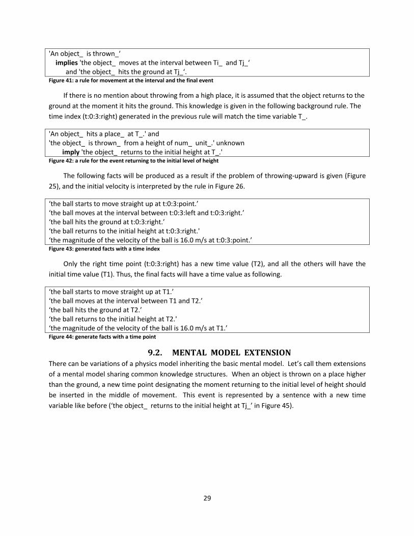
29

'An object_ is thrown_‘ implies 'the object_ moves at the interval between Ti_ and Tj_‘ and 'the object_ hits the ground at Tj_‘. Figure 41: a rule for movement at the interval and the final event

If there is no mention about throwing from a high place, it is assumed that the object returns to the

ground at the moment it hits the ground. This knowledge is given in the following background rule. The

time index (t:0:3:right) generated in the previous rule will match the time variable T_.

'An object_ hits a place_ at T_.' and 'the object_ is thrown_ from a height of num_ unit_.' unknown imply 'the object_ returns to the initial height at T_.' Figure 42: a rule for the event returning to the initial level of height

The following facts will be produced as a result if the problem of throwing-upward is given (Figure

25), and the initial velocity is interpreted by the rule in Figure 26.

‘the ball starts to move straight up at t:0:3:point.’ ‘the ball moves at the interval between t:0:3:left and t:0:3:right.’ ‘the ball hits the ground at t:0:3:right.’ ‘the ball returns to the initial height at t:0:3:right.' ‘the magnitude of the velocity of the ball is 16.0 m/s at t:0:3:point.’ Figure 43: generated facts with a time index

Only the right time point (t:0:3:right) has a new time value (T2), and all the others will have the

initial time value (T1). Thus, the final facts will have a time value as following.

‘the ball starts to move straight up at T1.’ ‘the ball moves at the interval between T1 and T2.’ ‘the ball hits the ground at T2.’ ‘the ball returns to the initial height at T2.' ‘the magnitude of the velocity of the ball is 16.0 m/s at T1.’ Figure 44: generate facts with a time point

9.2. MENTAL MODEL EXTENSION There can be variations of a physics model inheriting the basic mental model. Let’s call them extensions

of a mental model sharing common knowledge structures. When an object is thrown on a place higher

than the ground, a new time point designating the moment returning to the initial level of height should

be inserted in the middle of movement. This event is represented by a sentence with a new time

variable like before (‘the object_ returns to the initial height at Tj_’ in Figure 45).

30

Mental Model Extension –Throwing in a High Place

'An object_ was thrown_ upward_ from roof_ of a place2_, num1_ unitDist_ above a place_.' and

'the object_ starts to move at Ti_.' and

'the object_ hits the place_ at Tk_.' and

'Tj_ is a time point between Ti_ and Tk_.'

imply 'the object_ moves at the interval between Ti_ and Tj_.'

and 'the object_ returns to the level from which the object_ started to move at Tj_.‘

and 'the object_ moves straight down accelerating at the interval between Tj_ and Tk_.‘

Ti

Tk

Tj'the object_ starts to move straight up at Ti_.‘

'the object_ hits the ground at Tk_.‘

'the object_ returns to the initial height at Tj_.'

Figure 45: throwing upward on a high place

A background rule of the extended mental model produces facts about the event of the first half of

the movement (the first action in the right side of rule in Figure 46), the event about the returning to the

initial level of height (the second action), and the object movement down to the ground (the third

action). The given initial height is assigned to the displacement of the last half of the movement (the

fourth action). The initial time (Ti_) and the final time(Tk_) are given from facts generated by the basic

mental model.

'An object_ was thrown_ upward_ from roof_ of a place2_, num1_ unitDist_ above a place_' and 'the object_ starts to move at Ti_' and 'the object_ hits the place_ at Tk_' and 'Tj_ is a time point between Ti_ and Tk_' imply ‘the object_ moves at the interval between Ti_ and Tj_’ and ‘the object_ returns to the initial height at Tj_‘ and ‘the object_ moves straight down accelerating at the interval between Tj_ and Tk_‘ and ‘the magnitude of the displacement of the object_ is num_ unitDist_ at the interval between Tj_ and Tk_’ . Figure 46: the background rule for throwing upward in a high place.

A new time point should be created to the new variable for Tj_ designating the moment returning

to the initial height. But it cannot be created by simply introducing a new time variable in the right side

of the rule as done before. This time point has a constraint that it is between the starting point and the

ending point. This constraint is represented by ‘Tj_ is a time point between Ti_ and Tk_’, and it is given

to the condition of the rule. This condition matches a logic rule of a corresponding logic process (Figure

47). The logic rule has the internal representation for a time point in the right side (t:mid(Ti_, Tk_)), and

it is assigned to Tj_ when matched. The condition of the logic rule is represented in natural language.

‘Tj_ is a time point between Ti_ and Tk_.' if 'Tj_' = t:mid('Ti_', 'Tk_') Figure 47: a logic rule to generate a mid time point.

There can be further mental model extension from the previous extension. If a physics problem

asks about a quantity of an object related to the apex of the projectile movement, an event in the apex

with a new time point should be created. The event reaching the apex of the projectile movement is

represented by ‘the object_ is at the apex at Tj_’ (Figure 48).

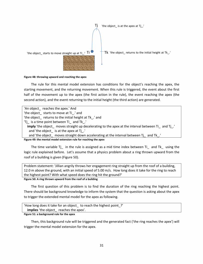
31

Mental Model Extension –Reaching the Apex

‘An object_ reaches the apex.' and

'the object_ starts to move at Ti_.' and

'the object_ returns to the level from which the object_ started to move at Tk_.' and

'Tj_ is a time point between Ti_ and Tk_.'

imply 'the object_ moves straight up decelerating to the apex at the interval between Ti_ and Tj_.'

and 'the object_ is at the apex at Tj_.'

and 'the object_ moves straight down accelerating at the interval between Tj_ and Tk_.'

Ti

Tj

Tk'the object_ starts to move straight up at Ti_.‘

'the object_ is at the apex at Tj_.‘

'the object_ returns to the initial height at Tk_.'

Figure 48: throwing upward and reaching the apex

The rule for this mental model extension has conditions for the object’s reaching the apex, the

starting movement, and the returning movement. When this rule is triggered, the event about the first

half of the movement up to the apex (the first action in the rule), the event reaching the apex (the

second action), and the event returning to the initial height (the third action) are generated.

‘An object_ reaches the apex.' And 'the object_ starts to move at Ti_.' and 'the object_ returns to the initial height at Tk_.' and 'Tj_ is a time point between Ti_ and Tk_.' imply 'the object_ moves straight up decelerating to the apex at the interval between Ti_ and Tj_.' and 'the object_ is at the apex at Tj_.' and 'the object_ moves straight down accelerating at the interval between Tj_ and Tk_.' Figure 49: the mental model extension rule for reaching the apex

The time variable Tj_ in the rule is assigned as a mid time index between Ti_ and Tk_ using the

logic rule explained before. Let’s assume that a physics problem about a ring thrown upward from the

roof of a building is given (Figure 50).

Problem statement: 'Jillian angrily throws her engagement ring straight up from the roof of a building, 12.0 m above the ground, with an initial speed of 5.00 m/s. How long does it take for the ring to reach the highest point? With what speed does the ring hit the ground?' Figure 50: A ring thrown upward from the roof of a building

The first question of this problem is to find the duration of the ring reaching the highest point.

There should be background knowledge to inform the system that the question is asking about the apex

to trigger the extended mental model for the apex as following.

‘How long does it take for an object_ to reach the highest point_?’ implies ‘the object_ reaches the apex’. Figure 51: a background rule for the apex

Then, this background rule will be triggered and the generated fact (‘the ring reaches the apex’) will

trigger the mental model extension for the apex.

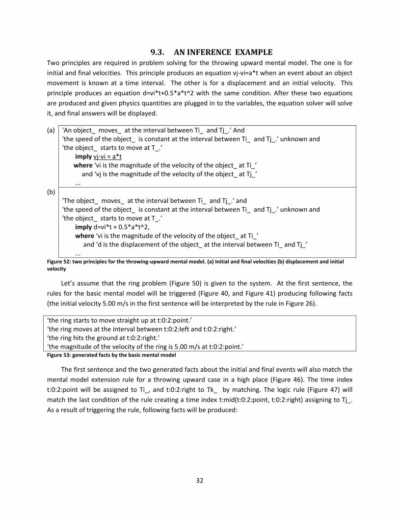
32

9.3. AN INFERENCE EXAMPLE Two principles are required in problem solving for the throwing upward mental model. The one is for

initial and final velocities. This principle produces an equation vj-vi=a*t when an event about an object

movement is known at a time interval. The other is for a displacement and an initial velocity. This

principle produces an equation d=vi*t+0.5*a*t^2 with the same condition. After these two equations

are produced and given physics quantities are plugged in to the variables, the equation solver will solve

it, and final answers will be displayed.

(a) 'An object_ moves_ at the interval between Ti_ and Tj_.' And 'the speed of the object_ is constant at the interval between Ti_ and Tj_.' unknown and 'the object_ starts to move at T_.‘ imply vj-vi = a*t where ‘vi is the magnitude of the velocity of the object_ at Ti_’ and ‘vj is the magnitude of the velocity of the object_ at Tj_’ ...

(b) 'The object_ moves_ at the interval between Ti_ and Tj_.' and 'the speed of the object_ is constant at the interval between Ti_ and Tj_.' unknown and 'the object_ starts to move at T_.‘ imply d=vi*t + 0.5*a*t^2, where ‘vi is the magnitude of the velocity of the object_ at Ti_’ and ‘d is the displacement of the object_ at the interval between Ti_ and Tj_’ ...

Figure 52: two principles for the throwing-upward mental model. (a) Initial and final velocities (b) displacement and initial velocity

Let’s assume that the ring problem (Figure 50) is given to the system. At the first sentence, the

rules for the basic mental model will be triggered (Figure 40, and Figure 41) producing following facts

(the initial velocity 5.00 m/s in the first sentence will be interpreted by the rule in Figure 26).

‘the ring starts to move straight up at t:0:2:point.’ ‘the ring moves at the interval between t:0:2:left and t:0:2:right.’ ‘the ring hits the ground at t:0:2:right.’ ‘the magnitude of the velocity of the ring is 5.00 m/s at t:0:2:point.’ Figure 53: generated facts by the basic mental model

The first sentence and the two generated facts about the initial and final events will also match the

mental model extension rule for a throwing upward case in a high place (Figure 46). The time index

t:0:2:point will be assigned to Ti_, and t:0:2:right to Tk_ by matching. The logic rule (Figure 47) will

match the last condition of the rule creating a time index t:mid(t:0:2:point, t:0:2:right) assigning to Tj_.

As a result of triggering the rule, following facts will be produced:

33

‘The ring moves at the interval between t:0:2:point and t:mid(t:0:2:point, t:0:2:right)' 'The ring returns to the initial height at t:mid(t:0:2:point, t:0:2:right)‘ ‘The ring moves straight down accelerating at the interval between t:mid(t:0:2:point, t:0:2:right) and t:0:2:right’ ‘the magnitude of the displacement of the ring is 12.0 m at the interval between t:mid(t:0:2:point, t:0:right) and t:0:2:right’ Figure 54: generated facts by the extended mental model

The first question sentence asking about the duration to the highest point will be interpreted

producing the fact that the ring reaches the apex by the rule in Figure 51. It will trigger the mental

model extension rule for the apex (Figure 49). Tj_ will be assigned with a new mid time point for the

apex between the initial time point (t:0:2:point) and the returning time point (t:mid(t:0:2:point,

t:0:2:right)), i.e. Tj_ becomes t:mid(t:0:2:point, t:mid(t:0:2:point, t:0:2:right)). The resulting facts

produced are as following:

‘The ring moves straight up decelerating to the apex at the interval between t:0:2:point and t:mid(t:0:2:point, t:mid(t:0:2:point, t:0:2:right))’ 'The ring is at the apex at t:mid(t:0:2:point, t:mid(t:0:2:point, t:0:2:right)).’ 'The ring moves straight down accelerating at the interval between t:mid(t:0:2:point, t:mid(t:0:2:point, t:0:2:right)) and t:mid(t:0:2:point, t:0:2:right)’ Figure 55: generated facts by the extended mental model for reaching the apex

The last two questions will be interpreted by the following background rules.

‘How long does it take for the object_ to reach a place_?’ and ‘the object_ starts to move at Ti_’ and ‘the object_ reaches the place_ at Tj_’ Imply ‘what is the displacement of the object_ at the interval between Ti_ and Tj_?’. With what speed does the object_ hit a place_?' and ‘the object_ hits a place_ at T_’ Imply ‘what is the magnitude of the velocity of the object_ at T_?’. Figure 56: background rules for the last two questions

Then, the two questions will be translated in physics representation that can match principles.

‘what is the displacement of the ring at the interval between t:0:2:point and t:mid(t:0:2:point, t:mid(t:0:2:point, t:0:2:right))?’ ‘what is the magnitude of the velocity of the ring at t:0:2:right?’ Figure 57: the two questioned translated in physics representation

34

t:0:2:point

t:mid(t:0:2:point, t:mid(t:0:2:point, t:0:2:right))

t:mid(t:0:2:point, t:0:2:right)‘

‘the ring starts to move straight up’

'the ring is at the apex‘

'The ring returns to the initial height‘

‘the ring moves at the interval.’

‘the ring hits the ground’

t:0:2:right

‘the magnitude of the velocity of the ringis 5.00 m/s.’

‘The ring moves at the interval '

‘The ring moves straight down accelerating’

‘The ring moves straight down accelerating‘

‘The ring moves straight up decelerating to the apex.‘what is the displacement of the ring?

‘The ring moves straight down accelerating ‘

‘what is the magnitude of the velocity of the ring?’

Figure 58: the produced facts with time index attached

Figure 58 depicts the produced facts with a time index attached on the trajectory of the object.

After the final time values are assigned, the final set of facts produced will be generated as Figure 59.

Additional facts such as direction of a vector and default facts about gravity can be driven from the

known facts, and they were added at the end of the set.

‘the ring starts to move straight up at T1.’ ‘the ring moves at the interval between T1 and T4.’ ‘the ring hits the ground at T4.’ ‘the magnitude of the velocity of the ring is 5.00 m/s at T1.’ ‘The ring moves at the interval between T1 and T3' 'The ring returns to the initial height at T3 ‘ ‘The ring moves straight down accelerating at the interval between T3 and T4’ ‘the magnitude of the displacement of the ring is 12.0 m at the interval between T3 and T4’ ‘The ring moves straight up decelerating to the apex at the interval between T1 and T2’ ‘The ring is at the apex at T2.’ ‘The ring moves straight down accelerating at the interval between T2 and T3’ ‘what is the displacement of the ring at the interval between T1 and T2?’ ‘what is the magnitude of the velocity of the ring at T4?’ ‘the direction of the velocity of the ring at T1 is 90 degrees.’ ‘the direction of the velocity of the ring at the interval between T1 and T2 is 90 degrees.’ ‘the direction of the velocity of the ring at the interval between T2 and T4 is 270 degrees.’ ‘the direction of the displacement of the ring at the interval between T1 and T2 is 90 degrees.’ ‘the direction of the displacement of the ring at the interval between T2 and t4 is 270 degrees.’

35

‘the magnitude of the velocity of the ring is 0 m/s at T2.’ ‘the magnitude of the displacement of the ring is 0 m at the interval between T1 and T3.’ ‘the magnitude of the displacement of the ring is 12.0 m at the interval between T1 and T4.’ ‘the location is near the earth.’ ‘the magnitude of gravitational acceleration on the earth is 9.8 m/s.’ ‘the magnitude of the acceleration of the ring is 9.8 m/s.’ ‘the direction of the acceleration of the ring is 90 degrees.’ Figure 59: generated facts at the end of the inference stage

This set of facts will trigger relevant principles in Figure 52. The given values (5.00 m/s, 12.0 m) are

assigned to the variables in the principles, and the following equations will be produced as a result.

Additional equations for time such as (Tik=Tij+Tik) and displacement (Dik=Dij+Dik) were not shown for

simplicity.

% for vj-vi = a*t (0 m/s)-(5.00 m/s) = -(9.8 m/s^2)*t12 (-5.00 m/s) – (0 m/s) =-(9.8 m/s^2)*t23 v4-(-5.00 m/s)=-(9.8 m/s^2)*t34 (-5.00 m/s)-(5.0 m/s)=-(9.8 m/s^2)*t13 v4-(5.00 m/s)=-(9.8m/s^2)*t14 % for d=vi*t + 0.5*a*t^2 d12=(5.00 m/s)*t12+0.5*(-9.8 m/s^2)*t12^2 d23=(0 m/s)*t23+0.5*(-9.8 m/s^2)*t23^2 (12 m)=(5.00 m/s)*t34+0.5*(-9.8 m/s^2)*t34^2 (0 m)= (5.00 m/s)*t13+0.5*(-9.8 m/s^2)*t13^2 (12 m)= (5.00 m/s)*t14+0.5*(-9.8 m/s^2)*t14^2 Figure 60: generated equations

Now the system calls the equation solver passing the set of equations to get final answers.

t12= (3.2 sec) v4= (8.00 m/s) Figure 61: the output of the equation solver

The final answer will be displayed with the natural language definition of the quantities asked in the

problem statement.

Answers: The duration at the interval between T1 and T2 is 3.2 sec. The magnitude of the velocity of the ring at T4 is 8.00 m/s. Figure 62: The final answers generated

The actual principles and variables are a little more complicated than the examples presented here.

For example, depending on the directions of an initial vector and a final vector, the sign of velocity in the

equations should change. However, they are not difficult to implement and they were not explained

here for simplicity.

36

This chapter has illustrated the complexity of a functional, extensible mental model. It is high, but

not overwhelming. Construction of an initial version of most mental model probably would need to be

done by an expert author e.g., a knowledge engineer rather than novice authors. However, extensions

to the mental model can be done by experienced authors. Building and extending mental models is one

of the main works required of Natural-K authors.

10.0. INFERENCE This chapter discusses the inference processes used by Natural-K which are done using knowledge

represented in natural language. The output of each step of inference is natural language, and it has an

advantage that the intermediate inference results can be read by anyone. It makes authoring tasks

easier allowing non-programmers to add and modify the knowledgebase. Also, the intermediate

inference results can be used to provide hints and explanations to a student being tutored.

The inference process includes three stages. In the first stage, inference is done only with non-

default knowledge. In the second stage, both default and non-default rules are used for inference. In

the third stage, additional inference for rules with a phrase variable is done.

10.1. FORWARD AND BACKWARD CHAINING Forward chaining is the basic method of inference used in the system, and backward chaining is

triggered in the middle of forward chaining in limited situations.

A physics problem statement is given to the system as input. The input triggers rules generating

facts inserting to the context memory. The generated facts trigger rules, and new facts are generated.

This process is repeated until no new fact is generated. Starting from given data (the problem

statement), the system finds all implied facts. It is called data-driven reasoning.

However, forward chaining has a problem generating too many facts not used in finding solutions.

This problem gets worse when the physics mental model has multiple time intervals. The number of

generated facts can grow fast as the number of time intervals increases. In case of four time points (T1,

T2, T3, and T4), there are six time intervals (i.e. T12, T23, T34, T13, T24, and T14). If facts for all the

intervals are produced, the size of facts becomes six times bigger. In case of six time points, there are 15

time intervals. In general, there are total n(n-1)/2 intervals when the biggest time point is Tn. The time

complexity of inference is O(N(r)*N(f)^N(c)), where N(r) is the number of rules, N(f) is the number of

facts, and N(c) is the average number of conditions per a rule. Not all the facts in the all the intervals are

needed in problem solving. Most of them are not used in problem solving just wasting computation

time if generated.

A truth rule checks validity of hypotheses not producing any new fact. Thus using them properly

can save computational time. The first example in Figure 17 is a truth rule used to reduce generated

facts due to sub time intervals. If it is added as an implication rule, facts in all combinations of time

intervals will be generated, and they will trigger other rules generating all other facts in the all intervals.

Most of the generated facts in the sub intervals will not be used in problem solving ending up wasting

37

computation time. The facts about object movements in required time intervals were already

generated when a mental model was created (Figure 41, Figure 46, and Figure 49). There is no need to

generate all facts in combination of sub time intervals if not required. Thus, adding the knowledge as a

truth rule (Figure 17) can save time not generating facts in all combinations of time intervals. Note that

a truth rule doesn’t trigger implication rules, and the system checks truth only using existing facts and

truth rules. Basically an author can determine which chaining (forward or backward) to apply for each

rule. Implication rules are for forward chaining, and truth rules are for backward chaining.

Backward chaining is triggered only when forward chaining reaches a dead end. When a condition

of an implication rule fails to find a matching fact from the context memory, the condition works as a

hypothesis, and the system tries to find a truth rule matched by the hypothesis. If there is no truth rule

matching, the rule fails to trigger. If a matching truth rule found, the system tries to validate the

conditions of the truth rule. The truth rule has conditions in the right side (as shown in Figure 16), and

they can be satisfied by existing facts. The conditions failing to find a satisfying fact will behave as

hypotheses and they will trigger other matching truth rules. It repeats until all hypotheses are satisfied

or there is no matching truth rule. This inference starts from a hypothesis and trigger other rules with

the hypothesis until all hypothesis are validated. This kind of inference is goal-driven reasoning.

Backward chaining was not applied from the input statement but triggered in the middle of forward

chaining because there is no way that the system can know the final goal (i.e. the sought quantities of a

problem) until the questions in the problem statement are interpreted. The problem statement is

interpreted line by line while reading it, and underlying implications are generated using forward

chaining first. It is a natural way for performing inferences while reading text.

10.2. DEFAULT KNOWLEDGE INFERENCE Evaluating the unknown conditions should not be done until the first inference stage using non-default

knowledge is completed. It is because it is possible that new facts satisfying the conditions can be

generated by other rules during the inference. Non-default rules are applied first for inference

generating facts, and default rules are applied next.

During compile time, rules are classified to default or non-default knowledge based on the type of

each condition. Inference in the first stage is done without default knowledge. Inference in the second

stage is done both with default and non-default knowledge.

Inference with default knowledge can generate unexpected results. Let’s assume that an unknown

fact A implies B, and the unknown fact B implies C. If the first rule is applied first, only B will be

generated. But if the second rule is applied first, both B and C will be generated. Figure 63 shows such

an example. The first rule is triggered when there is no mention about the location near a planet. It is

assumed that the location is near the earth if not mentioned about it. The second rule generates the

fact about zero gravity when the location is not near a planet and it is in space. If the first rule is applied

first, the fact about the location near the earth will be generated, and the second rule will fail due to the

first condition of it. If the second rule is applied first, the fact about zero gravity (‘objects have zero

gravity’) will be generated too.

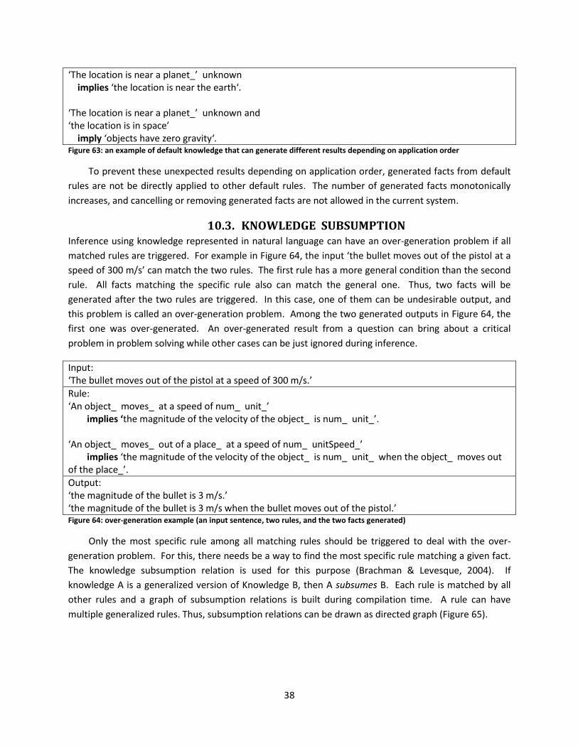
38

‘The location is near a planet_’ unknown implies ‘the location is near the earth‘. ‘The location is near a planet_’ unknown and ‘the location is in space’ imply ‘objects have zero gravity‘. Figure 63: an example of default knowledge that can generate different results depending on application order

To prevent these unexpected results depending on application order, generated facts from default

rules are not be directly applied to other default rules. The number of generated facts monotonically

increases, and cancelling or removing generated facts are not allowed in the current system.

10.3. KNOWLEDGE SUBSUMPTION Inference using knowledge represented in natural language can have an over-generation problem if all

matched rules are triggered. For example in Figure 64, the input ‘the bullet moves out of the pistol at a

speed of 300 m/s’ can match the two rules. The first rule has a more general condition than the second

rule. All facts matching the specific rule also can match the general one. Thus, two facts will be

generated after the two rules are triggered. In this case, one of them can be undesirable output, and

this problem is called an over-generation problem. Among the two generated outputs in Figure 64, the

first one was over-generated. An over-generated result from a question can bring about a critical

problem in problem solving while other cases can be just ignored during inference.

Input: ‘The bullet moves out of the pistol at a speed of 300 m/s.’

Rule: ‘An object_ moves_ at a speed of num_ unit_’ implies ‘the magnitude of the velocity of the object_ is num_ unit_’. ‘An object_ moves_ out of a place_ at a speed of num_ unitSpeed_’ implies ‘the magnitude of the velocity of the object_ is num_ unit_ when the object_ moves out of the place_’.

Output: ‘the magnitude of the bullet is 3 m/s.’ ‘the magnitude of the bullet is 3 m/s when the bullet moves out of the pistol.’ Figure 64: over-generation example (an input sentence, two rules, and the two facts generated)

Only the most specific rule among all matching rules should be triggered to deal with the over-

generation problem. For this, there needs be a way to find the most specific rule matching a given fact.

The knowledge subsumption relation is used for this purpose (Brachman & Levesque, 2004). If

knowledge A is a generalized version of Knowledge B, then A subsumes B. Each rule is matched by all

other rules and a graph of subsumption relations is built during compilation time. A rule can have

multiple generalized rules. Thus, subsumption relations can be drawn as directed graph (Figure 65).

39

Figure 65: Subsumption relations drawn as directed graph

During inference, a terminal node (i.e. the most specific rule in the tree) is selected and applied for

matching test. If it fails to match, then it goes up to the parent (i.e. the next specific rule) and tests

again. It is repeated until a matching rule is found. If there is no matching rule when it reaches the root

node, it moves to the next terminal node. The subsumption relations are compiled whenever the

knowledgebase is updated, and they don’t have to be compiled again until the next update. In this way,

the inference process avoids possible over-generations by applying only the most specific rule.

Subsumption relations are also used in a negation rule to suppress an undesired rule from

triggering (explained in chapter 6.1.3).

10.4. INFERENCE WITH PHRASE VARIABLES Rules with a phrase variable require special care for inference. Let’s assume that the current

knowledgebase is empty. In Figure 66, the time phrase ‘the ball returns to the initial height’ matches

the phrase variable does__, and the second condition is replaced with ‘the ball returns to the initial

height at time_’. But, it will fail to find a matching fact in the empty knowledgebase.

Input: 'What is the speed of the ball when the ball returns to the initial height?‘

‘What is the speed of an object_ when does__’ and ‘does__ at time_’

imply ‘what is the speed of an object_ at time_?’.

Context memory after default knowledge inference: {‘the ball returns to the initial height of the ball at t:0:1:left.’, …} Figure 66: an example of inference failure due to a time phrase

As shown in Figure 42, the fact about the event returning to the initial height is an action of a

default rule with an unknown condition, and this rule is applied during the default knowledge inference

stage. Let’s assume that the system finished the default knowledge inference stage producing the fact

about the event returning to the initial height (‘the ball returns to the initial height of the movement at

t:0:1:left.’). This fact will match the second condition of the rule in Figure 66, and it will become ‘the ball

returns to the initial height of the movement at t:0:1:left’. The first condition will be replaced with

‘what is the speed of the ball when the ball returns to the initial height of the movement’. But, the rule

Rule A

Rule C

Rule D

Rule B

Rule E

Rule F

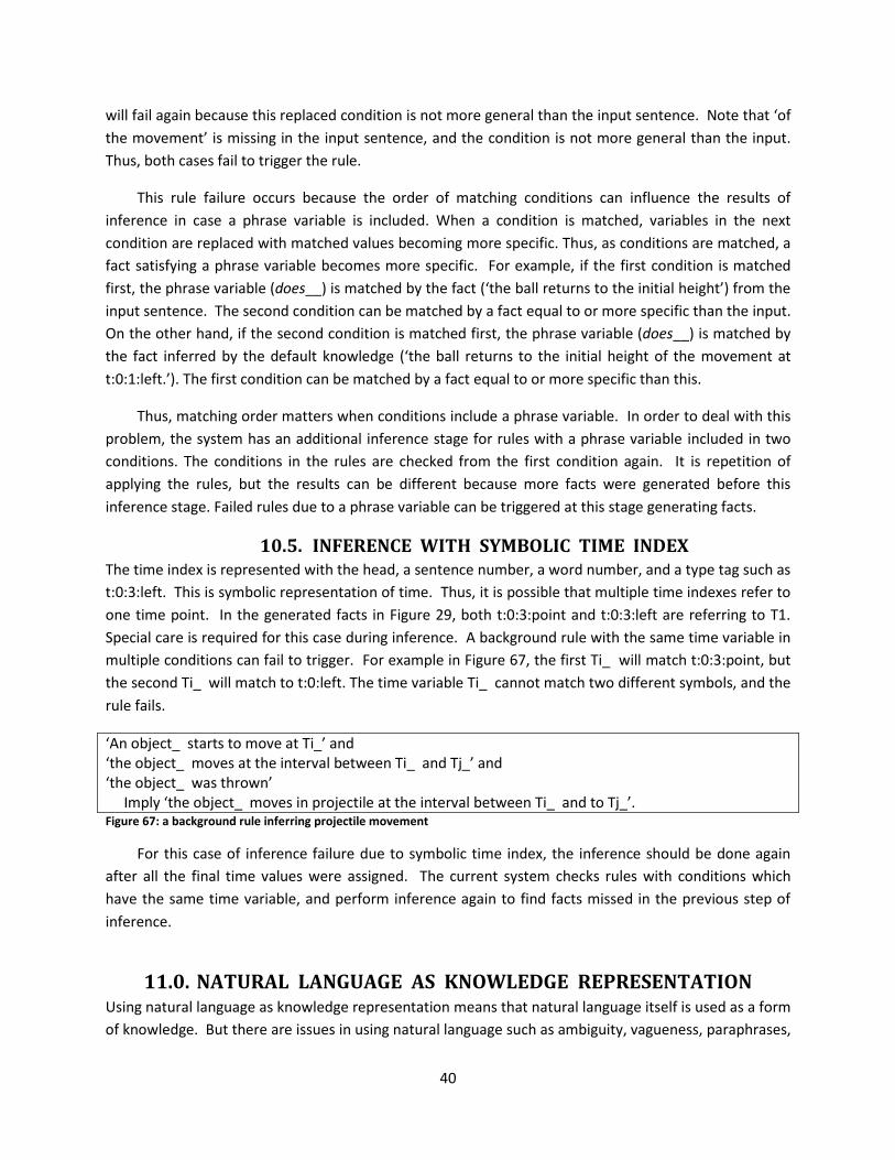
40

will fail again because this replaced condition is not more general than the input sentence. Note that ‘of

the movement’ is missing in the input sentence, and the condition is not more general than the input.

Thus, both cases fail to trigger the rule.

This rule failure occurs because the order of matching conditions can influence the results of

inference in case a phrase variable is included. When a condition is matched, variables in the next

condition are replaced with matched values becoming more specific. Thus, as conditions are matched, a

fact satisfying a phrase variable becomes more specific. For example, if the first condition is matched

first, the phrase variable (does__) is matched by the fact (‘the ball returns to the initial height’) from the

input sentence. The second condition can be matched by a fact equal to or more specific than the input.

On the other hand, if the second condition is matched first, the phrase variable (does__) is matched by

the fact inferred by the default knowledge (‘the ball returns to the initial height of the movement at

t:0:1:left.’). The first condition can be matched by a fact equal to or more specific than this.

Thus, matching order matters when conditions include a phrase variable. In order to deal with this

problem, the system has an additional inference stage for rules with a phrase variable included in two

conditions. The conditions in the rules are checked from the first condition again. It is repetition of

applying the rules, but the results can be different because more facts were generated before this

inference stage. Failed rules due to a phrase variable can be triggered at this stage generating facts.

10.5. INFERENCE WITH SYMBOLIC TIME INDEX The time index is represented with the head, a sentence number, a word number, and a type tag such as

t:0:3:left. This is symbolic representation of time. Thus, it is possible that multiple time indexes refer to

one time point. In the generated facts in Figure 29, both t:0:3:point and t:0:3:left are referring to T1.

Special care is required for this case during inference. A background rule with the same time variable in

multiple conditions can fail to trigger. For example in Figure 67, the first Ti_ will match t:0:3:point, but

the second Ti_ will match to t:0:left. The time variable Ti_ cannot match two different symbols, and the

rule fails.

‘An object_ starts to move at Ti_’ and ‘the object_ moves at the interval between Ti_ and Tj_’ and ‘the object_ was thrown’ Imply ‘the object_ moves in projectile at the interval between Ti_ and to Tj_’. Figure 67: a background rule inferring projectile movement

For this case of inference failure due to symbolic time index, the inference should be done again

after all the final time values were assigned. The current system checks rules with conditions which

have the same time variable, and perform inference again to find facts missed in the previous step of

inference.

11.0. NATURAL LANGUAGE AS KNOWLEDGE REPRESENTATION Using natural language as knowledge representation means that natural language itself is used as a form

of knowledge. But there are issues in using natural language such as ambiguity, vagueness, paraphrases,

41

etc. To be used in a computer system, it was generally believed that knowledge representation needs to

have properties such as verifiability, unambiguousness, standard (or canonical) form, inference with

variables, and expressiveness (Jurafsky & Martin, 2000).

Formal language such as predicate-argument structure satisfies the properties, and it is used in AI

systems in general. Formal language was regarded as representation of the deep meaning of natural

language, and natural language was regarded as surface level representation. Due to the problems in

using natural language, constrained natural language without ambiguity and vagueness was used in

previous studies (Fuchs, Kaljurand, & Kuhn, 2008). Basically constrained natural language is a kind of

formal language. Other studies using natural language as knowledge representation also focused on

formality (Iwanska & Shaprio, 2000) and applied to logic-related applications such as Boolean algebra

and logic reasoning(Shapiro, 2000).

Another approach is to transform natural language into formal language (Novak Jr., 1977) (Bundy,

Byrd, Luger, Mellish, & Palmer, 1979) (Ritter, 1998). The transformation approach has a problem that

principles were still written in computer program codes and they couldn’t be written by authors who

were not good at computer programming. Also transformation requires knowledge to translate natural

language to formal language, and such transformation knowledge was encoded in computer program

codes too. For example, templates were used to recognize natural language patterns and transform to

formal language, but only programmers were able to update such templates. It was one of the reasons

why this approach faced increasing difficulties as the size of the target world grows. The approach using

natural language representation is different from the transformation approach in the point that natural

language itself is used as knowledge representation and inference is done in natural language.

The knowledge representation presented in this thesis uses unconstrained free natural language

allowing ambiguity, vagueness, paraphrases, etc. Knowledge represented in natural language can be

verified using matching to existing facts. The proposed semantically binding variables enable inference

with variables. Expressiveness is not an issue because free natural language was allowed to represent

knowledge. These properties fulfill the requirements of knowledge representation to be used in a

computer system.

But the issue of ambiguity and paraphrases (i.e. no standard form) in natural language

representation should be addressed. In knowledge acquisition perspective, knowledge added in natural

language directly by humans has ambiguity and paraphrases. Thus, it is inevitable to allow ambiguity

and paraphrases in knowledge representation to unify knowledge used by humans and knowledge used

by computer systems.

Figure 68 shows examples of syntactic ambiguity. The prepositional phrase ‘on the hill’ can be

attached to ‘an airplane’ or ‘saw’. Depending on the attachment of the prepositional phrase, the

meaning of the sentence can be interpreted in different ways. If it is attached to ‘an airplane’, the

airplane was on the hill. If it is attached to ‘saw’, the man was on the hill. The two different

interpretations can be represented in formal language as saw(man, on(airplane, hill)) and saw(man,

42

airplane, on(hill)) respectively (Figure 68-(b)). Ambiguity resolution means choosing one out of the

different representations in formal language.

(a) A man saw an airplane on the hill.

(b) saw(man, on(airplane, hill)). saw(man, airplane, on(hill)).

Figure 68: an example of syntactic ambiguity (prepositional attachment). (a) an input sentence (b) two interpretations in formal language.

In case of natural language representation, ambiguity is not resolved by choosing an unambiguous

representation. The input sentence itself (Figure 68-(a)) is an ambiguous representation including the

two interpretations. In many cases, the ambiguity doesn’t have to be resolved. However, there can be

a situation that requires one to resolve the ambiguity. For example, it can be required to infer whether

the man was on the hill, or the airplane was on the hill in some physics problem. In Figure 69-(a), the

second sentence implies that the airplane was on the hill. Thus, the additional knowledge in the second

sentence provides information to resolve the ambiguity. The corresponding background rule uses the

two sentences to infer that the airplane was on the hill (in Figure 69-(b)). In the example Figure 69-(c),

the second sentence provides information about the airplane flying in the sky, and it can be inferred that

the man was on the hill. The corresponding background rule to infer it is shown in Figure 69-(d). In this

way, an inference rule using additional conditions can be used to resolve ambiguity. Notice that the

input sentence still has ambiguity and it was not replaced with an unambiguous representation like

formal language. In this way, inference with additional knowledge can have a role of ambiguity

resolution, and the issue of ambiguousness is a matter of inference in the natural language

representation.

(a) A man saw an airplane on the hill. The airplane crashed on the hill a long time ago.

(b) ‘An agent_ saw an object_ on a place_’ and ‘the object_ crashed on the place_ a long time ago’ Imply ‘the object_ is on the place_’.

(c) A man saw an airplane on the hill. The airplane was flying in the sky.

(d) ‘An agent_ saw an object_ on a place_’ and ‘The object_ was flying_’ Imply ‘the agent_ was on the place_’.

Figure 69: Ambiguity resolution in the natural language representation (a) the input sentence followed by another sentence (b) a background rule to infer that the airplane was on the hill (c) another example of the input sentence followed by another sentence (d) a background rule to infer that the man was on the hill.

The issues of vagueness and paraphrases are also just matter of inference in the natural language

representation. If the representation is vague, then there should be additional knowledge to perform

correct inference. If there are many paraphrases, then there should be background knowledge to

recognize the paraphrases. Generalized natural language representation using semantically binding

variables can recognize some extent of paraphrases. However in authoring perspective, adding

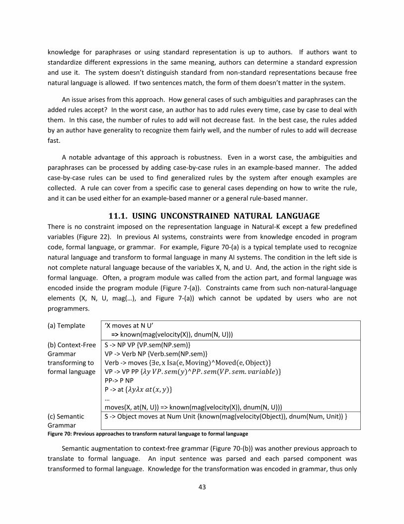
43

knowledge for paraphrases or using standard representation is up to authors. If authors want to

standardize different expressions in the same meaning, authors can determine a standard expression

and use it. The system doesn’t distinguish standard from non-standard representations because free

natural language is allowed. If two sentences match, the form of them doesn’t matter in the system.

An issue arises from this approach. How general cases of such ambiguities and paraphrases can the

added rules accept? In the worst case, an author has to add rules every time, case by case to deal with

them. In this case, the number of rules to add will not decrease fast. In the best case, the rules added

by an author have generality to recognize them fairly well, and the number of rules to add will decrease

fast.

A notable advantage of this approach is robustness. Even in a worst case, the ambiguities and

paraphrases can be processed by adding case-by-case rules in an example-based manner. The added

case-by-case rules can be used to find generalized rules by the system after enough examples are

collected. A rule can cover from a specific case to general cases depending on how to write the rule,

and it can be used either for an example-based manner or a general rule-based manner.

11.1. USING UNCONSTRAINED NATURAL LANGUAGE There is no constraint imposed on the representation language in Natural-K except a few predefined

variables (Figure 22). In previous AI systems, constraints were from knowledge encoded in program

code, formal language, or grammar. For example, Figure 70-(a) is a typical template used to recognize

natural language and transform to formal language in many AI systems. The condition in the left side is

not complete natural language because of the variables X, N, and U. And, the action in the right side is

formal language. Often, a program module was called from the action part, and formal language was

encoded inside the program module (Figure 7-(a)). Constraints came from such non-natural-language

elements (X, N, U, mag(…), and Figure 7-(a)) which cannot be updated by users who are not

programmers.

(a) Template ‘X moves at N U’ => known(mag(velocity(X)), dnum(N, U)))

(b) Context-Free Grammar transforming to formal language

S -> NP VP {VP.sem(NP.sem)} VP -> Verb NP {Verb.sem(NP.sem)} Verb -> moves { VP -> VP PP { PP-> P NP P -> at … moves(X, at(N, U)) => known(mag(velocity(X)), dnum(N, U)))

(c) Semantic Grammar

S -> Object moves at Num Unit {known(mag(velocity(Object)), dnum(Num, Unit)) }

Figure 70: Previous approaches to transform natural language to formal language

Semantic augmentation to context-free grammar (Figure 70-(b)) was another previous approach to

translate to formal language. An input sentence was parsed and each parsed component was

transformed to formal language. Knowledge for the transformation was encoded in grammar, thus only

44

programmers could update such knowledge. Semantic grammar (Figure 70-(c)) had more readable form

of grammar, but the knowledge required to transformation was still encoded in grammar and only

programmers could update it.

‘Constraints’ imposed on representation language is another name for knowledge modifiable only

by programmers. Unmodifiable knowledge works as constraints. Knowledge encoded in program code,

formal language, and grammar ends up being constraints to users. Even though the previous systems

were not intentionally designed to have constraints, their representation language was practically

constrained because users couldn’t modify the systems when it failed to accept an input. Thus,

designing a representation language for such knowledge to be modifiable by non-programmer was

essential for an unconstrained representation language. Adopting natural language to replace such

unmodifiable knowledge was tried for this purpose in this thesis.

Now, let’s compare to the representation in Natural-K using unconstrained natural language in a

form of rule. Both conditions and actions in a rule are represented in natural language, and they can be

updated by non-programmers. It is possible because no knowledge is encoded in program code,

grammar, or formal language:

‘An object_ moves_ at num_ unit_‘ implies ‘the magnitude of the velocity of the object_ is num_ unit_’ Figure 71: knowledge in unconstrained natural language

Even an ungrammatical sentence can be accepted if there is a rule with a condition of the same

sentence. For example, a random character sequence was given as an input in Figure 72-(a). The string

is not even English. However, let’s assume that this string can have a meaning of ‘nice to meet you’ in

an endangered language. An English parser will produce broken parse trees at the input, but it will

match the condition of the rule in Figure 72-(b) because the parser will generate exactly the same parse

trees though both are broken. Thus, the rule will be triggered generating the meaning of the string,

‘nice to meet you’. In previous transformation approaches, an input language was practically

constrained because users couldn’t modify a system to accept a given input if fails. In this unconstrained

language approach, if an input is not accepted, a user adds knowledge to make it accepted. So, there is

no constraint now.

(a) ‘uga uga uchacha’

(b) ‘uga uga uchacha’ implies ‘it is nice to meet you’.

Figure 72: accepting ungrammatical input. (a) an ungrammatical sentence (b) a rule to accept it.

Adopting this approach in principles (Figure 7-(b)) made all levels of knowledge representation

completely separated from program code. Instead of calling pre-encoded program modules, the rules

generate facts triggering other rules until the final outputs are generated. Inference is based on

matching facts and rules. No knowledge is encoded inside program code. Therefore, all levels of

background knowledge can be added by non-programmers in unconstrained natural language.

45

11.2. INTERNAL REPRESENTATION OF A SENTENCE Basically, for matching a specific sentence to a general sentence, Natural-K needs an internal

representation of a sentence. The internal representation should be able to include ambiguities of a

sentence, and it does not necessarily represent the deep meaning of a sentence. Resolving ambiguities

is done during inference using background knowledge. Although inference should be used to resolve

many cases of ambiguity and vagueness, a general mechanism can be used for certain fairly regular

syntactic variations. Paraphrases created due to syntactic variations such as passive and active voice can

be normalized in the internal representation.

11.3. AMBIGUITY Ambiguity of natural language includes syntactic ambiguity and semantic ambiguity. Both ambiguities

can be represented in the internal representation of a sentence. This section explains the internal

representation for the two types of ambiguity.

11.3.1. Syntactic Ambiguity

One of the problems in language analysis is that the current status of parsing accuracy is not good

enough for many practical applications in spite of recent advances. The system uses a general purpose

dependency parser developed for this research. The number of generated parse trees depends on the

grammar rules that have been given. Too many parse trees can be generated by the parser when loose

parsing rules are applied, while a correct parse tree is often not generated when strict parsing rules are

applied. This section discusses some common syntactic problems and the ways to handle them.

The ambiguity due to prepositional attachment shown in Figure 69 is at the syntax level. The parse

tree when the prepositional phrase (‘on the hill’) is attached to the noun (‘airplane) is shown in the right

top of Figure 73. The other parse tree when the prepositional phrase is attached to the verb (‘saw’) is

shown in the right bottom of the figure. The internal representation of the sentence is the union of the

two parse trees. Thus, a parse chart containing all possible trees is used as internal representation of a

sentence (in the left part of Figure 73). A chart parser generates a chart including all parsing candidates,

and output of the chart parser is used as the internal representation of the sentence.

46

A dependency chart can include multiple ambiguous parse treesThe dependency chart is only used for internal process in the system.

A man saw an airplane on the hill.

A man

(comp)

saw

(prep)

an airplane on

(dt)

hill.

(subject)

(dt)

(n)

(dt)

the

A man

(comp)

saw

(prep)

an airplane on

(dt)

hill.

(subject)

(dt)

(n)

(dt)

the

A man

(comp)

saw

(prep)

an airplane on

(dt)

hill.

(subject)

(dt)

(n)

(dt)

the

(prep)

A dependency chart

Dependency Trees

Figure 73: A chart containing all parse trees generated is used as internal representation of a sentence.

Suppose that both the input sentence (Figure 68-(a)) and the first condition of the background rule

(Figure 69-(b) and Figure 69-(d)) have prepositional attachment ambiguity. Then both parse trees of the

input sentence can match the both parse trees of the condition of the rule. In this example, it doesn’t

matter whether the preposition ‘on’ is attached to ‘saw’ or ‘airplane’ because they have the same

ambiguities. Let’s suppose another case that both the input sentence and a condition of rule are

ambiguous, but they share only one parse tree. This is a loose case of matching. That is, the system

regards two sentences as matched if one of parse trees from each side is matched.

The internal representation using parse chart is used only to see whether two sentences match or

not, and it is not used for other purposes in general such as information extraction. The main purpose

of parsing is to extend the matching scope of sentences from general to specific sentences (“a man saw

it” vs. “a young man saw it”) and syntactic variations (passive vs. active).

11.3.2. Semantic Ambiguity

Another linguistic ambiguity is from semantics. For example, the word ‘saw’ includes multiple senses:

1. The past tense of ‘see’

2. A toothed device for cutting

3. …

Among the available senses, no. 1 is the closest meaning of ‘saw’ in the statement in the previous

examples (Figure 68). The system looks up word senses only for a variable word (attached by ‘_’).

Matching fails immediately if two word roots are not identical and both are non-variable words. When

one of words is a variable, the variable word should be a hypernym (with a broader meaning) of the

other one. Each variable word should have word senses for this reason. A domain expert is not

47

expected to be able to assign word sense because it is not an easy task due to the fine-grained senses of

WordNet.

The system looks up WordNet and assigns word senses to a variable word after parsing.

Information about a sentence form and related senses is used, however basically word sense

disambiguation is not applied, and all senses are assigned to a variable word. During matching, if one of

the senses for each word matches, then the two words are regarded as matched. Word roots are used

in matching to avoid the variations of tense, number, and gender. Articles (‘a’, ‘an’, ‘the’) and

punctuation were ignored in matching.

11.4. SYNTACTIC NORMALIZATION There are a million different ways to say something in natural language. Syntactic variations are part of

such variations. Normalizing syntactic variations including active vs. passive voice, relative phrases,

conjunctive forms were implemented.

11.4.1. Active vs. Passive Voice (does vs. is done)

A passive form of English can be rewritten in an active form without significantly changing the meaning.

The passive form of a sentence should be able to match the active form of it or vice versa. A parse tree

of a sentence doesn’t match directly to that of the corresponding passive sentence. Normalization is

applied to convert them to be in the same form. In order to normalize a passive form to an active form,

normalization links were inserted into the parse chart. Figure 74 shows two normalization links inserted,

pushed-(object)->crate and pushed-(subject)->man. For sentence matching, the system compares two

sentences using normalization links if available. In this way, a passive sentence can match the

corresponding active sentence after the normalization process.

“A crate was pushed by a man.”

A crate

(pp)

was

(prep)

pushed by

(dt)

man.

(Subject)

(dt)

(n)

a

A dependency chart

A crate

(pp)

was

(prep)

pushed by

(dt)

man.

(Subject)

(dt)

(n)

a

A normalized dependency chart

(Subject)

(object)

(normalization link)

Figure 74: Syntactic normalization of a passive form

11.4.2. Relative Clause (A which B)

There are multiple forms of a relative clause conveying the same meaning. In the example of Figure 75-

(a), the relative clause ‘who pushed a crate’ was rewritten as ‘pushing a crate’. In Figure 75-(b), the

relative clause ‘which a man pushed’ was rewritten without ‘which’.

(a) ‘A man who pushed a crate’ ‘A man pushing a crate’

48

(b) ‘A crate which a man pushed’ ‘A crate a man pushed’

Figure 75: a relative clause and its variation

A normalization link is inserted to a relative clause to maintain the same syntactic structure. Now, the

normalized parse tree in Figure 76 can match its variations.

A man

(v)

who

(object)

pushed crate.

(relative)

(dt)

(dt)

a

A normalized dependency chart

(subject)

(normalization links)

Figure 76: sentence normalization for relative clause

11.4.3. Conjunctive phrase (A and B)

Special care is needed for conjunctive phrases because they can bring about many syntactic ambiguities.

In order to reduce such ambiguities, only the last conjunct (i.e. the last word connected to ‘and’) is

connected to the head during parsing. For example, when “A man pushed a crate and a desk” is parsed,

pushed-(object)->desk is included in the parse tree, but not pushed-(object)->crate. Although this

reduces the number of parse trees, it raises a problem that it cannot be directly understood that ‘a crate’

is an object of the verb ‘pushed’ too because there is no direct link between them. So, a normalization

link is inserted between the verb and the other conjuncts, as in Figure 77. As a result, the parse chart

can be understood as both “A man pushed a crate” and “A man pushed a desk”.

A man

(v)

(object)

pushed desk

(dt)(dt)

a

A normalized dependency chart

(object)

(normalization links)

crate

(dt)

a and

(left_conj) (conj)

Figure 77: Sentence normalization for conjunctive phrase.

11.4.4. Inserting a Normalization Link to Chart

Although a normalization link can be simply inserted into a parse tree, it is risky to insert it into a parse

chart. A chart is union of multiple parse trees, so inserting a link between two nodes can affect other

parse trees. In the case of Figure 78, there are two parse trees where “by a man” is attached to either

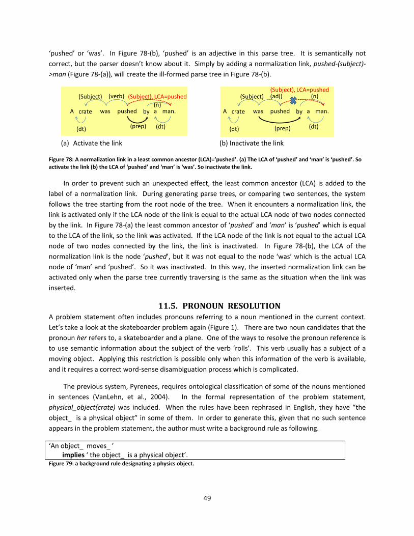
49

‘pushed’ or ‘was’. In Figure 78-(b), ‘pushed’ is an adjective in this parse tree. It is semantically not

correct, but the parser doesn’t know about it. Simply by adding a normalization link, pushed-(subject)-

>man (Figure 78-(a)), will create the ill-formed parse tree in Figure 78-(b).

A crate

(verb)

was

(prep)

pushed by

(dt)

man.

(Subject)

(dt)

(n)a

(Subject), LCA=pushed

A crate

(comp)

was

(prep)

pushed by

(dt)

man.

(Subject)

(dt)

(n)a

(Subject), LCA=pushed

A crate

(pp)

was

(prep)

pushed by

(dt)

man.

(Subject)

(dt)

(n)

a

(Subject)

A crate

(adj)

was

(prep)

pushed by

(dt)

man.

(Subject)

(dt)

(n)

a

(Subject), LCA=pushed

(a) Activate the link (b) Inactivate the link

Figure 78: A normalization link in a least common ancestor (LCA)=’pushed’. (a) The LCA of ‘pushed’ and ‘man’ is ‘pushed’. So activate the link (b) the LCA of ‘pushed’ and ‘man’ is ‘was’. So inactivate the link.

In order to prevent such an unexpected effect, the least common ancestor (LCA) is added to the

label of a normalization link. During generating parse trees, or comparing two sentences, the system

follows the tree starting from the root node of the tree. When it encounters a normalization link, the

link is activated only if the LCA node of the link is equal to the actual LCA node of two nodes connected

by the link. In Figure 78-(a) the least common ancestor of ‘pushed’ and ‘man’ is ‘pushed’ which is equal

to the LCA of the link, so the link was activated. If the LCA node of the link is not equal to the actual LCA

node of two nodes connected by the link, the link is inactivated. In Figure 78-(b), the LCA of the

normalization link is the node ‘pushed’, but it was not equal to the node ‘was’ which is the actual LCA

node of ‘man’ and ‘pushed’. So it was inactivated. In this way, the inserted normalization link can be

activated only when the parse tree currently traversing is the same as the situation when the link was

inserted.

11.5. PRONOUN RESOLUTION A problem statement often includes pronouns referring to a noun mentioned in the current context.

Let’s take a look at the skateboarder problem again (Figure 1). There are two noun candidates that the

pronoun her refers to, a skateboarder and a plane. One of the ways to resolve the pronoun reference is

to use semantic information about the subject of the verb ‘rolls’. This verb usually has a subject of a

moving object. Applying this restriction is possible only when this information of the verb is available,

and it requires a correct word-sense disambiguation process which is complicated.

The previous system, Pyrenees, requires ontological classification of some of the nouns mentioned

in sentences (VanLehn, et al., 2004). In the formal representation of the problem statement,

physical_object(crate) was included. When the rules have been rephrased in English, they have “the

object_ is a physical object” in some of them. In order to generate this, given that no such sentence

appears in the problem statement, the author must write a background rule as following.

‘An object_ moves_ ’ implies ‘ the object_ is a physical object’. Figure 79: a background rule designating a physics object.

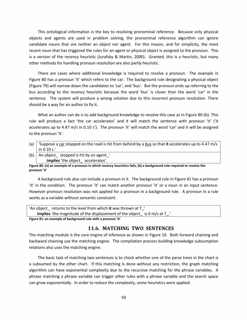
50

This ontological information is the key to resolving pronominal reference. Because only physical

objects and agents are used in problem solving, the pronominal reference algorithm can ignore

candidate nouns that are neither an object nor agent. For this reason, and for simplicity, the most

recent noun that has triggered the rules for an agent or physical object is assigned to the pronoun. This

is a version of the recency heuristic (Jurafsky & Martin, 2000). Granted, this is a heuristic, but many

other methods for handling pronoun resolution are also partly heuristic.

There are cases where additional knowledge is required to resolve a pronoun. The example in

Figure 80 has a pronoun ‘it’ which refers to the car. The background rule designating a physical object

(Figure 79) will narrow down the candidates to ‘car’, and ‘bus’. But the pronoun ends up referring to the

bus according to the recency heuristic because the word ‘bus’ is closer than the word ‘car’ in the

sentence. The system will produce a wrong solution due to this incorrect pronoun resolution. There

should be a way for an author to fix it.

What an author can do is to add background knowledge to resolve this case as in Figure 80-(b). This

rule will produce a fact ‘the car accelerates’ and it will match the sentence with pronoun ‘it’ (‘it

accelerates up to 4.47 m/s in 0.10 s’). The pronoun ‘it’ will match the word ‘car’ and it will be assigned

to the pronoun ‘it’.

(a) 'Suppose a car stopped on the road is hit from behind by a bus so that it accelerates up to 4.47 m/s in 0.10 s.'

(b) An object_ stopped is hit by an agent_' implies 'the object_ accelerates'.

Figure 80: (a) an example of a pronoun in which recency heuristics fails, (b) a background rule required to resolve the pronoun ‘it’

A background rule also can include a pronoun in it. The background rule in Figure 81 has a pronoun

‘it’ in the condition. The pronoun ‘it’ can match another pronoun ‘it’ or a noun in an input sentence.

However pronoun resolution was not applied for a pronoun in a background rule. A pronoun in a rule

works as a variable without semantic constraint.

‘An object_ returns to the level from which it was thrown at T_’ implies ‘the magnitude of the displacement of the object_ is 0 m/s at T_.’ Figure 81: an example of background rule with a pronoun ‘it’

11.6. MATCHING TWO SENTENCES The matching module is the core engine of inference as shown in Figure 10. Both forward chaining and

backward chaining use the matching engine. The compilation process building knowledge subsumption

relations also uses the matching engine.

The basic task of matching two sentences is to check whether one of the parse trees in the chart is

a subsumed by the other chart. If this matching is done without any restriction, the graph matching

algorithm can have exponential complexity due to the recursive matching for the phrase variables. A

phrase matching a phrase variable can trigger other rules with a phrase variable and the search space

can grow exponentially. In order to reduce the complexity, some heuristics were applied.

51

The first heuristic is that the matching always starts from the root nodes of both sentences’ parse

trees. The main verb of a sentence becomes the head in a dependency parse tree. Normally, the head

verb becomes the root of the parse tree. So matching normally starts with the main verbs of two

sentences.

The second is that, the same phrase variable is not allowed to be applied twice. For example, once

a rule ‘if__ does__’ was applied, this rule is not applied again inside the phrase. Nested if-phrases are

not allowed.

12.0. STUIDES AND RESULTS

12.1. GOALS AND EVALUATION PLAN There are mainly two goals of the studies here. The one is to see whether the expressive power of the

natural language representation is good enough to represent physics problems. The physics problems

from Pyrenees and physics textbooks were added to Natural-K in order to test its expressive power, and

the result was shown in the knowledge adding task in section 12.2. The other goal is to see the

generality of the representation. If the generalized representation cannot cover broad ranges of

knowledge patterns, specific knowledge has to be added every time. It is expected that the number of

added rules will converge to near zero as more problems are added if the generalized representation

works well.

In the ideal state of authoring task, most physics problems would be understood and solved

correctly. If the system doesn’t understand or misunderstands a problem, and thus generates

unexpected results, the user can rephrase the input statement until the problem is correctly solved.

However, it might take several attempts at rewording the problem before the reworded problem is

interpreted correctly, but it should not be allowed to replace the whole problem statement without

limit. Thus, determining if the system is in the no-new-knowledge state requires stating a criterion that

bounds the min-edit distance at rewording. Min-edit distance is defined by the sum of the number of

additions, deletions, and modifications of words. If 90% of problems are solved with less than 15 edits,

then it can be said that the system is virtually in the no-new-knowledge state.

This criterion would need to be tested separately for each mental model, such as the throw-upward

mental model, and it would need to be tested with authors who are not familiar with the internal

workings of the system. This would be a difficult to test on a large set of problems. Thus, more feasible

tests were applied. First, the problems were added until the author got five physics problems correctly

solved without a new rule. Presumably, the number of problems added required to reach the “real” no-

new-knowledge state would be a (linear?) function of this number, e.g., twice as many. This was done

within the throw-upward mental model. Rewording was not allowed during this test except for: (1)

changing units e.g., feet and miles to meters; (2) dividing a long sentence connected with “and”

conjunctions into separate sentences; and (3) deleting formatting such as numbering the parts (a), (b),…

in a multi-part problem. This test was shown in Figure 84 in section 12.2

52

Second, it was estimated how many mental models were found in a typical physics chapter. As

mentioned earlier, each mental model requires a different set of knowledge to correctly interpret a

given problem, and a chapter of a physics textbook usually includes problems in different mental models.

It could also be that the same mental models appear in multiple chapters (e.g., a Throw-upward model

might appear in both the kinematics chapter and the dynamics chapter), which would also save writing

some rules. The number of mental models per chapter of three chapters was assessed. This estimation

was shown in section 12.4.

Lastly, four authors who are not involved in this project were recruited so that we can see whether

their performance is similar to the system developer when the system has reached the no-new-

knowledge state. In particular, if the number of added rules added by the system developer converges

to near zero, can the non-developer authors do so as well? If the system developer can add a problem

by rewording it, can the non-developer authors do so as well? Thus, a set of problems in the throw-

upward mental model were used for measuring convergence. For the mental model, the adding of

physics problems continued until at least ten problems were found in textbooks that require only

rewording in order to be translated. Both the system developer and the recruited authors’ min-edit

distance were counted. This test was shown in section 12.3 and 12.5.

12.2. Knowledge Adding Task The expressiveness of knowledge representation was assessed by the knowledge adding task. Three

test sets of physics problems were added. The first includes 37 problems in Pyrenees in three physics

domains (kinematics, statics, and dynamics). The second comprises 32 problems in kinematics from a

physics textbook (Young & Freedman, 2004). The last includes 23 problems in throw-upward mental

models from several textbooks. Questions asking a qualitative answer, using a figure or table,

continuation of a previous question, derivation or introducing equations, and comparing two events

requiring multiple mental models were not included in the previous system, Pyrenees, and they were

not included in this test too.

1. 37 problems in Pyrenees (Kinematics (19 problems), Statics(9), and Dynamics(9))

2. 32 problems in Chapter 2 of Young&Freedman’s textbook (Kinematics)(Young & Freedman, 2004)

3. 23 problems in throw-upward mental model (Young & Freedman, 2004)(Serway, Vuille, & Faughn,

2009)(Amstutz, 2001)(Crowell, 2000)(Fogiel, 1976 )(Kumar, 2008)(Blatt, 1989)(Ewen, Nelson, &

Schurter, 1996)

The three sets of physics problems were successfully added to the system by the system developer,

and the system was able to solve them all correctly after updating and debugging the knowledgebase. A

total of 92 problems, and 562 background rules (including 42 logic rules, and 45 principle rules) were

added. The successfully added physics problems from three different physics domains (Kinematics,

Statics, and Dynamics) show that the representation power is not limited in one domain. The physics

problems from the textbook (the second set) were also added and solved correctly. It shows that the

proposed natural language representation has enough representation power to solve problems from

textbook.

53

This knowledge adding task was done by the system developer because it took long time with

intensive efforts to build the initial knowledgebase. This task requires repeated knowledge debugging

and regression tests after update. The recruited users spent only 4 to 9 hours for their participation,

and it was too short for the knowledge adding task for the whole three test sets. In the real

environment, the initial knowledgebase will be built by the system developer, and domain experts will

participate in after the initial knowledgebase is built.

Now the remaining issue is about how fast the system converges to the no-new-knowledge-state.

The convergence graph presented next (Figure 82) shows the number of principles and background rules

added. The 37 Pyrenees problems were added starting from an empty knowledgebase. An average of

10.3 rules were added per a problem. This suggests that the number of required rules is small enough

that an author can feasibly add them. Building from the knowledgebase of the Pyrenees’ problems, the

32 Young and Freedman’s textbook problems were added next. An average of 4.5 rules were added per

a problem gently converging down (Figure 83; note the change in y-axis scale). It supports the initial

hypothesis that the amount of knowledge to add per problem in an ITS is small enough for an author to

add.

Figure 82: the number of rules added for each physics problem in Pyrenees

0

5

10

15

20

25

30 principle rules added

background rules

54

Figure 83: the number of rules added for each physics problem in Young&Freeman’s Textbook

However, the convergence was not as fast as initially expected. Analysis of the added rules

suggested that the slow convergence was due to the fragmentation of background knowledge into a

number of mental models.

Thus, to see the generality of representation power, the 23 physics problems in a single mental

model (throw-upward) were added. They were added to the knowledge base attained at then end of

Figure 74, where the last of the Young & Freeman problems was added. Figure 84 shows the number of

added rules for each problem. Among the knowledge used in this mental model, the rules added in the

previous sets were counted at the first usage, and most of them were counted in the first problem

(exp2_7_pp60). As the figure shows, it converged faster, and five of the problems were automatically

solved without adding a new rule. It shows that the number of rules that authors must add converges

faster to near zero given that all the problems are in the same mental model. This suggests that the

number of automatically solved problems without adding a new rule will increase as more problems are

added.

0

1

2

3

4

5

6

7

8

9 principle rules added

background rules added

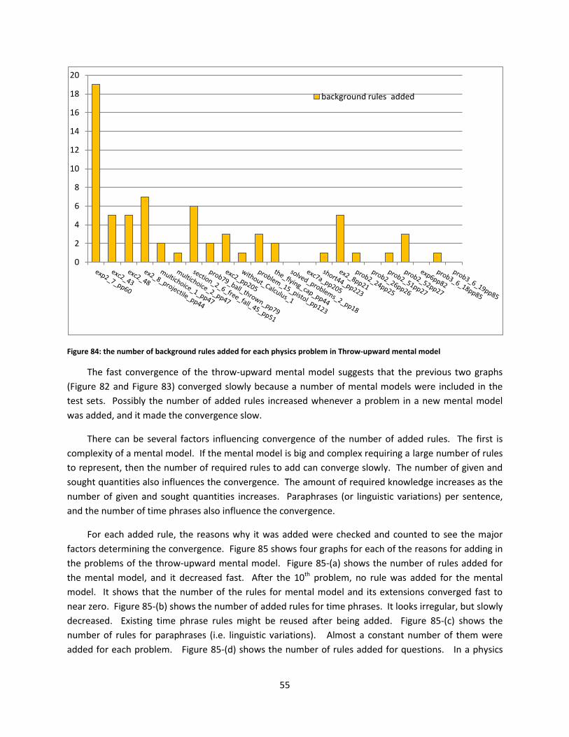
55

Figure 84: the number of background rules added for each physics problem in Throw-upward mental model

The fast convergence of the throw-upward mental model suggests that the previous two graphs

(Figure 82 and Figure 83) converged slowly because a number of mental models were included in the

test sets. Possibly the number of added rules increased whenever a problem in a new mental model

was added, and it made the convergence slow.

There can be several factors influencing convergence of the number of added rules. The first is

complexity of a mental model. If the mental model is big and complex requiring a large number of rules

to represent, then the number of required rules to add can converge slowly. The number of given and

sought quantities also influences the convergence. The amount of required knowledge increases as the

number of given and sought quantities increases. Paraphrases (or linguistic variations) per sentence,

and the number of time phrases also influence the convergence.

For each added rule, the reasons why it was added were checked and counted to see the major

factors determining the convergence. Figure 85 shows four graphs for each of the reasons for adding in

the problems of the throw-upward mental model. Figure 85-(a) shows the number of rules added for

the mental model, and it decreased fast. After the 10th problem, no rule was added for the mental

model. It shows that the number of the rules for mental model and its extensions converged fast to

near zero. Figure 85-(b) shows the number of added rules for time phrases. It looks irregular, but slowly

decreased. Existing time phrase rules might be reused after being added. Figure 85-(c) shows the

number of rules for paraphrases (i.e. linguistic variations). Almost a constant number of them were

added for each problem. Figure 85-(d) shows the number of rules added for questions. In a physics

0

2

4

6

8

10

12

14

16

18

20

background rules added

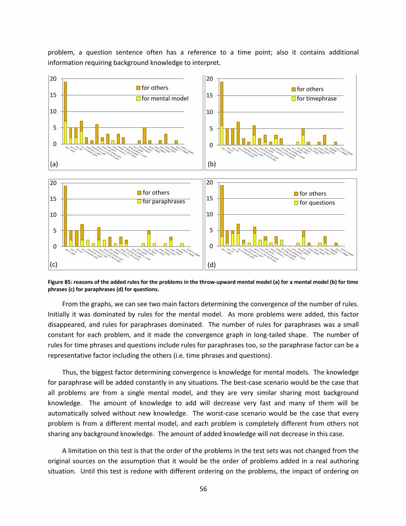
56

problem, a question sentence often has a reference to a time point; also it contains additional

information requiring background knowledge to interpret.

Figure 85: reasons of the added rules for the problems in the throw-upward mental model (a) for a mental model (b) for time phrases (c) for paraphrases (d) for questions.

From the graphs, we can see two main factors determining the convergence of the number of rules.

Initially it was dominated by rules for the mental model. As more problems were added, this factor

disappeared, and rules for paraphrases dominated. The number of rules for paraphrases was a small

constant for each problem, and it made the convergence graph in long-tailed shape. The number of

rules for time phrases and questions include rules for paraphrases too, so the paraphrase factor can be a

representative factor including the others (i.e. time phrases and questions).

Thus, the biggest factor determining convergence is knowledge for mental models. The knowledge

for paraphrase will be added constantly in any situations. The best-case scenario would be the case that

all problems are from a single mental model, and they are very similar sharing most background

knowledge. The amount of knowledge to add will decrease very fast and many of them will be

automatically solved without new knowledge. The worst-case scenario would be the case that every

problem is from a different mental model, and each problem is completely different from others not

sharing any background knowledge. The amount of added knowledge will not decrease in this case.

A limitation on this test is that the order of the problems in the test sets was not changed from the

original sources on the assumption that it would be the order of problems added in a real authoring

situation. Until this test is redone with different ordering on the problems, the impact of ordering on

0

5

10

15

20

for others

for mental model

0

5

10

15

20

for others

for timephrase

0

5

10

15

20

for others

for paraphrases

0

5

10

15

20

for others

for questions

(a) (b)

(c) (d)

57

convergence can only be estimated. Nonetheless, the order of the problems would probably not

significantly affect the result in a single mental model. This is because the problems share the same

domain knowledge for the mental model which is the biggest factor determining the convergence. The

knowledge for the mental model has to be added first regardless of problem order. The order of

difficulty of problems in a single mental may have minor influence on the graph due to this reason.

In case of problems with multiple mental models, the order of difficulty of problems also would not

have influence outside a mental model because the share of domain knowledge among different mental

models is limited. For example, the mental model for projectile movement doesn’t share knowledge

with the mental model for straight movement on the ground. A possible influence of ordering can be in

mental model extensions. If problems of an extended mental model are added first, knowledge for its

basic mental is added together and it can result in a little faster convergence inside the mental model.

However, many mental models have various extensions, and knowledge for the extensions is not shared

except inherited mental models. Also in a textbook, it is usual that easy problems in a basic mental

model come first, and difficult problems in extended mental models come later. The order of the

problems in the test set followed this usual order of textbook to reflect the real situation of authoring.

12.3. Rewording Task Theoretically, the system with an empty knowledgebase can be given to non-programmers, and they

can start to build the knowledgebase. However, in practical situations, the initial knowledge building

tasks should be done by a system developer or knowledge engineers. In particular, the developer

creates the initial versions of the background knowledge. The developer also defines the set of natural

language definitions for the physics representation. This phase has to be done by the system developer

because extensive debugging is needed. When the developer has created an operational version of the

knowledgebase that suffices for, say, dozens of problems per physics chapter, then adding new

problems should require adding only a small set of new background rules and principles. This can be

done by domain experts with modest knowledge engineering skills. Eventually, the system reaches the

desired no-new-knowledge-state, wherein domain experts without programming skill can add most

problems without adding any new knowledge to the system.

The number of rules added for the mental model (Figure 85-(a)) decreased fast, and they were not

added after the tenth problem. Rules for a mental model include time variables creating a new time

index (Figure 26, Figure 28, Figure 40, Figure 41, etc.), and they cannot be added by simply rewording a

problem statement. This suggests that the problems after the tenth problem (total 13 problems) could

be added only by rewording. In order to test the no-new-knowledge-state, a rewording task was done.

In rewording task, words in a problem statement are modified, deleted, or new words are added so

that the sentence can match the condition of a relevant rule. Figure 86-(a) is the problem statement of

from the test sets. The background rule to be triggered is in Figure 46, but it was not triggered because

the input sentence didn’t match the condition of the rule. So, the problem statement had to be

reworded. Figure 86-(b) is the reworded statement (underlines were added only for readers of this

thesis). Figure 86-(c) shows that two words (‘tall’, and ‘with’) were deleted, two words (‘does’->’is’, and

‘strike’->’hits’) were modified, and nine words were added. The min-edits distance was 13.

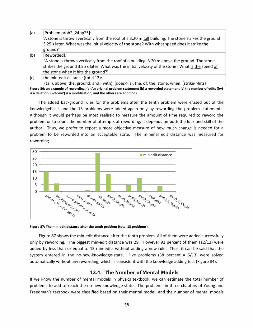
58

(a) [Problem prob2_24pp25]: 'A stone is thrown vertically from the roof of a 3.20 m tall building. The stone strikes the ground 3.25 s later. What was the initial velocity of the stone? With what speed does it strike the ground?'

(b) [Reworded]: 'A stone is thrown vertically from the roof of a building, 3.20 m above the ground. The stone strikes the ground 3.25 s later. What was the initial velocity of the stone? What is the speed of the stone when it hits the ground?'

(c) the min-edit distance (total 13): (tall), above, the, ground, and, (with), (does->is), the, of, the, stone, when, (strike->hits)

Figure 86: an example of rewording. (a) An original problem statement (b) a reworded statement (c) the number of edits ((w) is a deletion, (w1->w2) is a modification, and the others are addition)

The added background rules for the problems after the tenth problem were erased out of the

knowledgebase, and the 13 problems were added again only by rewording the problem statements.

Although it would perhaps be most realistic to measure the amount of time required to reword the

problem or to count the number of attempts at rewording, it depends on both the luck and skill of the

author. Thus, we prefer to report a more objective measure of how much change is needed for a

problem to be reworded into an acceptable state. The minimal edit distance was measured for

rewording.

Figure 87: The min-edit distance after the tenth problem (total 13 problems).

Figure 87 shows the min-edit distance after the tenth problem. All of them were added successfully

only by rewording. The biggest min-edit distance was 29. However 92 percent of them (12/13) were

added by less than or equal to 15 min-edits without adding a new rule. Thus, it can be said that the

system entered in the no-new-knowledge-state. Five problems (38 percent = 5/13) were solved

automatically without any rewording, which is consistent with the knowledge adding test (Figure 84).

12.4. The Number of Mental Models If we know the number of mental models in physics textbook, we can estimate the total number of

problems to add to reach the no-new-knowledge state. The problems in three chapters of Young and

Freedman’s textbook were classified based on their mental model, and the number of mental models

0

5

10

15

20

25

30 min edit distance

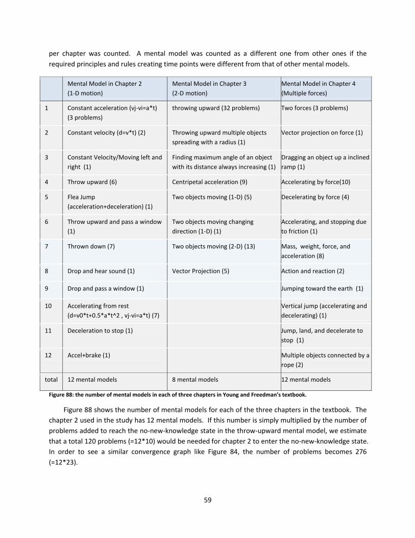
59

per chapter was counted. A mental model was counted as a different one from other ones if the

required principles and rules creating time points were different from that of other mental models.

Mental Model in Chapter 2

(1-D motion)

Mental Model in Chapter 3

(2-D motion)

Mental Model in Chapter 4

(Multiple forces)

1 Constant acceleration (vj-vi=a*t)

(3 problems)

throwing upward (32 problems) Two forces (3 problems)

2 Constant velocity (d=v*t) (2) Throwing upward multiple objects

spreading with a radius (1)

Vector projection on force (1)

3 Constant Velocity/Moving left and

right (1)

Finding maximum angle of an object

with its distance always increasing (1)

Dragging an object up a inclined

ramp (1)

4 Throw upward (6) Centripetal acceleration (9) Accelerating by force(10)

5 Flea Jump

(acceleration+deceleration) (1)

Two objects moving (1-D) (5) Decelerating by force (4)

6 Throw upward and pass a window

(1)

Two objects moving changing

direction (1-D) (1)

Accelerating, and stopping due

to friction (1)

7 Thrown down (7) Two objects moving (2-D) (13) Mass, weight, force, and

acceleration (8)

8 Drop and hear sound (1) Vector Projection (5) Action and reaction (2)

9 Drop and pass a window (1) Jumping toward the earth (1)

10 Accelerating from rest

(d=v0*t+0.5*a*t^2 , vj-vi=a*t) (7)

Vertical jump (accelerating and

decelerating) (1)

11 Deceleration to stop (1) Jump, land, and decelerate to

stop (1)

12 Accel+brake (1) Multiple objects connected by a

rope (2)

total 12 mental models 8 mental models 12 mental models

Figure 88: the number of mental models in each of three chapters in Young and Freedman’s textbook.

Figure 88 shows the number of mental models for each of the three chapters in the textbook. The

chapter 2 used in the study has 12 mental models. If this number is simply multiplied by the number of

problems added to reach the no-new-knowledge state in the throw-upward mental model, we estimate

that a total 120 problems (=12*10) would be needed for chapter 2 to enter the no-new-knowledge state.

In order to see a similar convergence graph like Figure 84, the number of problems becomes 276

(=12*23).

60

However, it is a very rough estimation close to the worst case because 7 out of the 12 mental

models have only one problem, and only three mental models (throwing-upward, throwing-downward,

and accelerating-from-rest) have more than three problems. The three major mental models cover 62

percent of the problems (=(6+7+7)/32) in the chapter. If estimated in the same way before, they can

reach the no-new-knowledge state after adding 30 (=3*10) problems, and 15 problems (3*5) can be

solved without a new rule if 39 (=3*13) more problems are added. The major three mental models are

more complex than others because they include multiple time intervals with model extensions requiring

additional knowledge, and there can be sharable knowledge between the mental models. But, these

factors were not considered in the estimation suggesting that the actual number of required rules is

smaller than the numbers presented in this paragraph.

The problems in chapter 3 and chapter 4 have similar distribution. Chapter 3 has eight mental

models, but two mental models have 67 percent of problems (=(32+13)/67). Chapter 4 has twelve

mental models, but two mental models have 53 percent of problems (=(10+8)/34). If the proportion of

the problems in the throwing-upward mental model can be applied to the other mental models, the 67

percent problems of chapter 3 can reach the no-new-knowledge state after adding 20 problems (=2*10),

and 10 problems (2*5) can be solved without a new rule if 26 problems (=2*13) are added more. In the

same way, the 53 percent of chapter 4 can reach the no-new-knowledge state after adding 20 problems

(=2*10), and 10 problems (=2*5) can be solved without a new rule if adding 26 problems more (2*13).

12.5. STUDIES WITH RECRUITED USERS The previous studies were done by the system developer. The system developer has deep

understanding about the system and the knowledge representation. There is a possibility that users

who are not involved in the system development can show different behaviors. One of the purposes of

using natural language representation is to develop a system for which users don’t have to learn a new

knowledge representation. Practically speaking, the system can be given to users after the initial

knowledgebase is built by a system developer. Thus, the physics problems in the no-knowledge-state

(Figure 87) were used to test whether the users can do the same authoring task done by the system

developer.

Four people who took a college physics class were recruited for the study. The subjects had never

seen or used the system before the studies, and the idea of using a natural language representation was

explained in the beginning of the studies. The studies included three sessions, i.e. demo session,

training session, and test session. In the demo session, the system execution solving the skateboarder

problems (Figure 9) was shown to the subjects, and the basic mechanism of inference using the

background knowledge and principles were explained briefly. For the training session, three physics

problems created to help subjects to understand the authoring task were used to train them. The

system developer showed the subjects how to add, debug, and update knowledge using the first training

problem, and the subjects just watched how he was doing. Next, the subjects added the second training

problem with help of the system developer. The subjects added the third training problem with help of

the system developer too, but it was skipped with short explanations if they were already good at the

second problem.

61

In the test session, the subjects were asked to add the 13 physics problems used in the rewording

study (the problems in Figure 87). First, they were asked to add all 13 problems by rewording. After

that, they were asked to roll back to the original problem and add rules instead of rewording.

Figure 89-(a) is one of the physics problems from the test set. Figure 89-(b) is the statement

reworded by one of the recruited users. The added, deleted, or modified words were underlined only

for readers of this thesis. At the first execution, the system failed in solving the problem. So, he had to

figure out what was wrong. It is not trivial because there are many possible reasons of a failure. In the

first line of the statement, he had to find a relevant rule to be triggered in the knowledgebase. This was

not an easy task because there were already hundreds rules in the knowledgebase. The given problem

must have a mental model throwing upward in a high place. He searched using several keywords such

as ‘roof’, ‘building’, and ‘above’ to find a relevant rule for the mental model. The relevant rule to be

triggered was shown in Figure 46. He compared the first condition of the rule and the first line of input,

and replaced the word ‘vertically’ with ‘upward’. In this way, he repeated rewording any suspicious

phrases in the problem statement until a solution by the system was correct. After the problem was

solved correctly, he was asked to roll back to the original problem, and he added rules instead of

rewording as shown in Figure 89-(c). He added specific rules because it was easier than adding

generalized rules. The system will be able to generalize them after enough number of specific rules is

collected. This approach helps to minimize the burdens of authors to check regression of previously

added knowledge.

(a) [Problem ex2_8pp21]: 'A stone is thrown vertically from the roof of a building 50.0 m above the ground. The stone strikes the ground 5.00 s after it is thrown. With what speed was it thrown? What was the maximum height it attained? With what speed did it strike the ground?'

(b) [Reworded]: 'A stone is thrown straight upward from the roof of a building, 50.0 m above the ground.' 'The duration is 5.00 s when the stone is in the air.' 'What is the initial speed of the stone?' 'How high does it go?' 'What is the speed of the stone when it hits the ground?'

(c) [Added Rules]: 'A stone is thrown vertically from the roof of a building 50.0 m above the ground.' implies 'A stone is thrown straight upward from the roof of a building, 50.0 m above the ground'. 'The stone strikes the ground 5.00 s after it is thrown. ' implies 'The duration is 5.00 s when the stone is in the air.'. 'With what speed was it thrown?' implies 'What is the initial speed of the stone?'. 'what was the maximum height it attained?' implies 'How high does it go?'. 'with what speed did it strike the ground?' implies 'What is the speed of the stone when it hits the ground?'.

Figure 89: An example of (a) a problem statement, (b) a reworded statement, and (c) added rules by the subject4

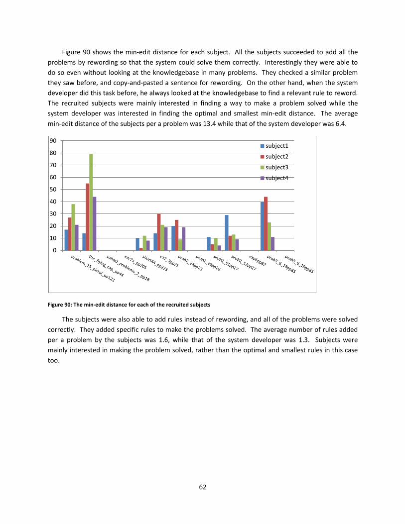
62

Figure 90 shows the min-edit distance for each subject. All the subjects succeeded to add all the

problems by rewording so that the system could solve them correctly. Interestingly they were able to

do so even without looking at the knowledgebase in many problems. They checked a similar problem

they saw before, and copy-and-pasted a sentence for rewording. On the other hand, when the system

developer did this task before, he always looked at the knowledgebase to find a relevant rule to reword.

The recruited subjects were mainly interested in finding a way to make a problem solved while the

system developer was interested in finding the optimal and smallest min-edit distance. The average

min-edit distance of the subjects per a problem was 13.4 while that of the system developer was 6.4.

Figure 90: The min-edit distance for each of the recruited subjects

The subjects were also able to add rules instead of rewording, and all of the problems were solved

correctly. They added specific rules to make the problems solved. The average number of rules added

per a problem by the subjects was 1.6, while that of the system developer was 1.3. Subjects were

mainly interested in making the problem solved, rather than the optimal and smallest rules in this case

too.

0

10

20

30

40

50

60

70

80

90 subject1

subject2

subject3

subject4

63

Figure 91: The number of rules added by each subject

The average min-edit distance, time spent, and the number of trials for rewording for each problem

was shown in Figure 92. The time spent at the problems solved without a new rule was not zero

because of the first execution time before rewording was included. The subjects executed the system to

solve a given problem to see whether it was solved without a new rule, and they reworded it only when

it was not correctly solved. The number of trials is the count of the execution command of the system

minus 1, and the minus 1 was to exclude the first execution before rewording. The average number of

trials was 1.2, and the biggest number of trials was four. The execution time to solve a problem was

about 4 to 7 minutes. It took 4 to 46 minutes in average across the subjects to complete the rewording

task for a problem starting from reading a problem statement.

Figure 92: The min-edit distance, time spent, and the number of trials in average across the subjects.

0

1

2

3

4

5

6 subject1

subject2

subject3

subject4

0

10

20

30

40

50

60 min edit distance

Time for rewording (minutes)

number of trials for rewording

64

The authoring task adding rules instead of rewording was easier because the subjects already did it

by rewordings. Most of the time, this task could be done by copying the original and reworded

sentences and pasting into a rule. When a problem was solved without a new rule in the rewording task,

this task was skipped resulting in zero time spent. All subjects were able to do this task in one or two

trials, and the biggest number of trials was three.

Figure 93: The number of rules added, time spent, and the number of trials in average across subjects

All the subjects were able to do the authoring tasks both by rewording and by adding rules like the

system developer did. Except for the facts that the time spent, the number of added rules, and the

number of trials of the subjects were larger than that of the system developer, they were able to do the

authoring tasks with the knowledge represented in natural language.

At the end of the final session, the subjects were asked to answer three questions. The first

question was about the most difficult thing they faced during the authoring tasks. All the subjects

expressed difficulties in figuring out why a problem was not solved and what to do next. This is a

common difficulty of authoring with a sizable knowledgebase. They didn’t point out any difficulty

related to the system or methods proposed in this thesis at this question.

Question 1: What was the most difficult thing while you were doing the authoring tasks?

Subject Answer to Question1:

1 Knowing what to do when I encountered a problem. (A user manual might help.)

2 When a problem was not solved, it was difficult to figure out why.

3 Finding relevant rules in the KB.

4 Knowing which phrases is going to be accepted Figure 94: Question1

The second question was about usability of the system by non-programmer users. Three of the

subjects answered that the system could be used by non-programmers. They said that they were able

to do the authoring task using previously authored examples, and they did it using only natural language.

0

2

4

6

8

10

12

14

16 the number of rules added

time to add rules (minutes)

trials for adding rules

65

One of the four subjects said maybe. He was concerned that it could be difficult to recover when a user

got stuck. When a knowledgebase is large and complex, a user can gets stuck in the middle of debugging

knowledge. However, this concern was not about the methodology of the proposed idea using natural

language as knowledge representation, but a concern about difficulty of authoring task itself.

Question 2: Now, you finished your authoring task. Did you get impression that any users who don't know computer programming can use the system?

Subject Answer to Question2

1 Yes. (Previous examples were important to figure out how to use. So, if more good examples are available, it will be easier to use)

2 Yes. (I was able to author problems only using natural language.)

3 Yes.

4 Maybe. (When it gets stuck, it can be difficult to recover) Figure 95: Question2

The third question was about a suggestion for improvement for the system. One subject said that

using multiple windows was confusing, and suggested integrating into a single window interface.

Another suggested a tool to help search matchable rules in the knowledgebase. He pointed out a

difficulty in finding relevant rules that can be alleviated by such a tool. The others suggested improving

the execution speed.

Question 3: Do you have suggestions to improve or change the system?

Subject Answer to Question3

1 Integrate multiple windows into a single window interface.

2 A tool to help search matchable rules in KB.

3 Faster execution speed

4 Faster execution speed Figure 96: Question3

In summary, all the four recruited subjects were able to add the problems either by rewording or

adding knowledge. They agreed that the system could be used by non-programmers, and the difficulties

they faced using the system were not specifically related to the approach using the proposed natural

language representation.

13. DISCUSSION The experimental results showed that physics problems in three different areas (kinematics, statics,

dynamics) were successfully represented in natural language, and the system solved them correctly.

Note that problems in statics are mainly about forces acting on an object. The required principles and

domain knowledge in statics are different from that in kinematics which mainly dealing with velocity and

acceleration of a moving object. This suggests that the natural language representation has enough

expressive power and is not restricted to one domain. Basically, if knowledge in domain problems can

be represented in natural language, this approach can be applied.

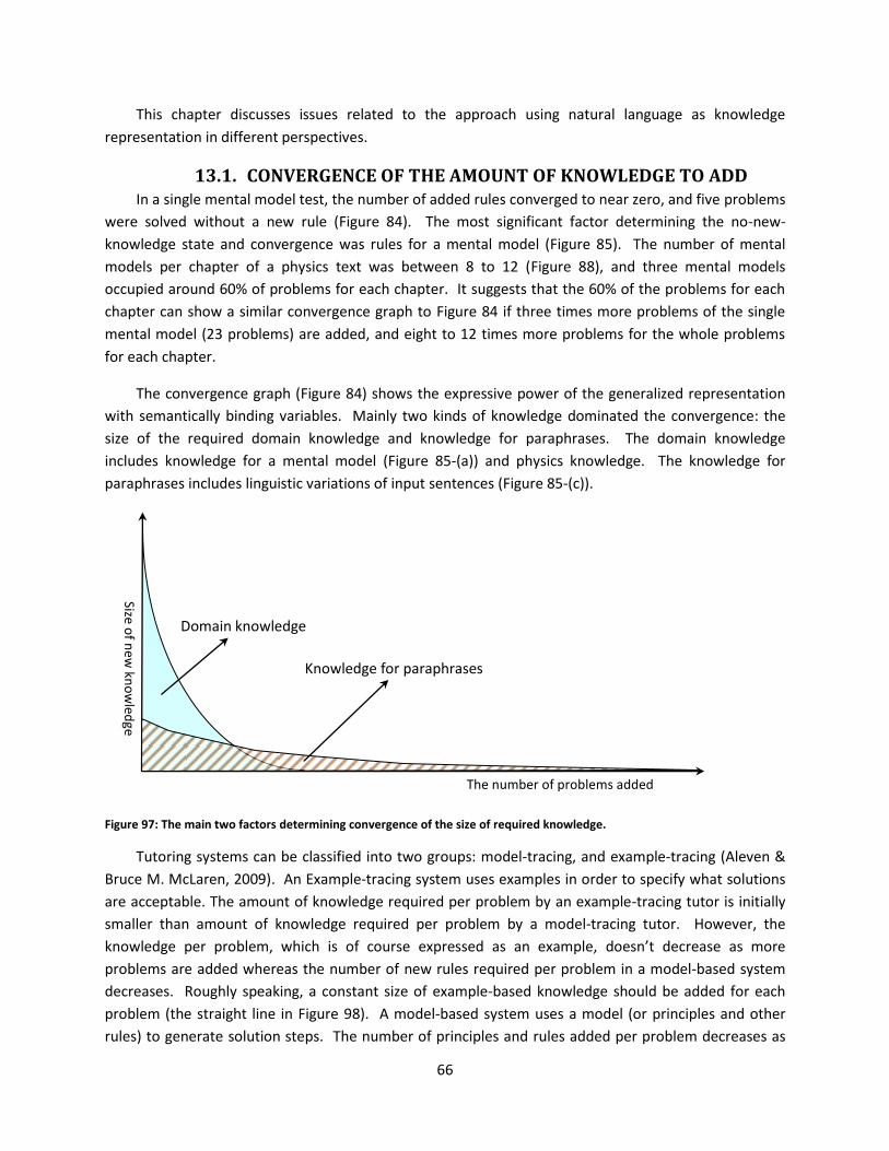
66

This chapter discusses issues related to the approach using natural language as knowledge

representation in different perspectives.

13.1. CONVERGENCE OF THE AMOUNT OF KNOWLEDGE TO ADD In a single mental model test, the number of added rules converged to near zero, and five problems

were solved without a new rule (Figure 84). The most significant factor determining the no-new-

knowledge state and convergence was rules for a mental model (Figure 85). The number of mental

models per chapter of a physics text was between 8 to 12 (Figure 88), and three mental models

occupied around 60% of problems for each chapter. It suggests that the 60% of the problems for each

chapter can show a similar convergence graph to Figure 84 if three times more problems of the single

mental model (23 problems) are added, and eight to 12 times more problems for the whole problems

for each chapter.

The convergence graph (Figure 84) shows the expressive power of the generalized representation

with semantically binding variables. Mainly two kinds of knowledge dominated the convergence: the

size of the required domain knowledge and knowledge for paraphrases. The domain knowledge

includes knowledge for a mental model (Figure 85-(a)) and physics knowledge. The knowledge for

paraphrases includes linguistic variations of input sentences (Figure 85-(c)).

Figure 97: The main two factors determining convergence of the size of required knowledge.

Tutoring systems can be classified into two groups: model-tracing, and example-tracing (Aleven &

Bruce M. McLaren, 2009). An Example-tracing system uses examples in order to specify what solutions

are acceptable. The amount of knowledge required per problem by an example-tracing tutor is initially

smaller than amount of knowledge required per problem by a model-tracing tutor. However, the

knowledge per problem, which is of course expressed as an example, doesn’t decrease as more

problems are added whereas the number of new rules required per problem in a model-based system

decreases. Roughly speaking, a constant size of example-based knowledge should be added for each

problem (the straight line in Figure 98). A model-based system uses a model (or principles and other

rules) to generate solution steps. The number of principles and rules added per problem decreases as

Knowledge for paraphrases

Domain knowledge

The number of problems added

Size of n

ew

kno

wled

ge

67

more problems are added. If the model-tracing tutor uses a formal representation, then the amount of

knowledge per problem never reaches zero because the problem statements themselves must be

expressed in a formal knowledge representation. The Formal representations in Figure 6-(a) translating

the problem statement are such an example to be added for every problem. The middle curve in Figure

98 depicts the size of knowledge for model-tracing systems using formal language. Thus, for both

example-based and model-based tutoring systems, the size of required new knowledge added per

problem never converges to zero.

In contrast, the size of the required new knowledge to add per problem in Natural-K can converge

to zero. An ITS can be built on Natural-K, and it can be a model-based system although it can be used

like an example-based system if only specific knowledge is used without a principle. The information

given in a problem statement (given and sought quantities, etc.) is interpreted by background

knowledge. The background knowledge in generalized representation using semantically binding

variables recognizes general patterns of sentences. Initially more new knowledge can be required than

model-based systems using formal language, but the size of the required new knowledge can converge

to zero as the number of added problems increases. The lowest curve in Figure 98 depicts the amount

of knowledge for the approach using natural language representation. The amount of knowledge to add

in a single mental model in Figure 84 showed a similar convergence, and it is expected that the overall

convergence in a domain will show such a convergence graph.

Figure 98: comparison of three types of tutoring systems and the size of knowledge to add.

Therefore, after the initial knowledgebase is built by knowledge engineers, domain experts can add

problems by adding a small size of knowledge. The natural language based approach has two

advantages in authoring perspectives. The one is that users can understand knowledge directly without

learning new representation such as formal language or programming language. The other is that the

size of new knowledge to add can converge to zero.

Model-based using formal language

Example-based

Natural language

based

The number of problems added

Am

ou

nt o

f new

kno

wled

ge

68

13.2. A New Dimension of ITS Types An ITS can be built on Natural-K. Natural-K acquires a new type of knowledge to read problems

statements. Background knowledge to interpret naïve representation mapping to physics

representation was not used in previous ITSs. This knowledge can be used to generate explanations and

hints. This type of knowledge is important in tutoring, especially in understanding a given problem

before applying and solving. Understanding a problem includes tasks to find mapping from a given

problem statement to a proper mental model and relevant principles. As shown in section 13.7, an

object released out of a moving vehicle has an initial velocity that is the same to the vehicle’s. This

knowledge is important for understanding the problem, but it was largely ignored in previous systems

because this type of knowledge was not encoded when manually translating to formal language, and

because it was difficult to generate hints and explanations from formal language even if encoded. Thus,

a new kind of tutoring system can be built on it strengthening understanding parts.

The previous types of ITSs (example-based and model-based) were classified based on the types of

knowledge they used to tutor students. The behaviors of the two types of ITSs in a tutoring mode can

be exactly the same even if they use different types of knowledge (examples vs. models). But, their

behaviors in authoring are fundamentally different. As shown in Figure 98, the amount of knowledge to

add in each of the three types of tutors (example-based, model-based, and NL(Natural Language)-based)

distinguishes them. The distinctive characteristics of a NL-based tutor come from the fact that it has

background knowledge to understand problem statements.

However, classifying all ITSs into the three classes (example-based, model-based, and NL-based) is

inappropriate. Both examples-based and model-based tutors also can use a natural language

representation. A new classification is appropriate such as FL(Formal language)-based vs. NL-based

tutors. It means that the NL vs. FL is a new dimension orthogonal to the example vs. model dimension.

A new classification I propose is a two dimensional classification for ITSs as following.

FL-based NL-based

Model-based Pyrenees, Fermi, Newton, CASCADE, AURA

ITS based on Natural-K

Example-based CTAT Figure 99: A new dimension of ITS types

An ITS based on Natural-K will be a NL-model-based one. If a NL-based ITS uses only background

knowledge without a principle and a mental model, it will belong to a NL-example-based one. The

behaviors of model-based and example-based systems in a tutoring mode are not fundamentally

different because they are based on the same kind of knowledge. But, a NL-based ITS has a new kind of

knowledge mapping a problem statement to principles which is important in problem understanding

rather than problem solving. Thus, a NL-based ITS can have strength in generating explanations and

hints. It will be discussed in section 13.7.

13.3. Separating Knowledge from Computer Programming The biggest breakthrough made in this thesis is that the knowledge level was completely separated from

computer programming level. In previous approaches using formal language or transformation

69

approach, parts of knowledge were still encoded in program codes because they should trigger

principles with conditions encoded in programming code (Figure 7-(a)). The parts of knowledge plugged

into the conditions were predefined because the program code cannot be changed easily. A definition

of a quantity and variable was encoded in programming code too, and they were used in conditions of a

principle. In case of transformation approach (Novak Jr., 1977) (Bundy, Byrd, Luger, Mellish, & Palmer,

1979), knowledge required for transformation was encoded in programming code too. For example,

transformation modules were designated in grammar, and called during parsing. In case of a template-

based transformation approach, predefined templates were used to recognize sentence patterns; the

condition part of template is a sentence pattern using predefined terms, and the action part is formal

language or program code to be triggered. The approach using constrained natural language (Fuchs,

Kaljurand, & Kuhn, 2008) also used predefined (or constrained) forms of input because the knowledge

has to be plugged in program code to trigger program modules (or principles) at the end.

Thus, principles and their conditions encoded in programming code were the reasons for using

restricted or constrained knowledge representation in previous studies. By representing principles and

their conditions in natural language, it became possible to use free natural language for knowledge

representation, thus completely separating the knowledge level from the programming level. Therefore,

it became possible for authors to use free natural language without learning how to represent

knowledge formally. Note that that generalized natural language representation is readable both by

humans and computers.

There is virtually no predefined form of physics quantities such as velocity and acceleration in the

proposed natural language representation. Only time, numbers and units in generalized representation

were predefined (as shown in Figure 22). The other quantities gain their meaning from the principles in

natural language (Figure 7-(b)). When domain experts add principles, they add definitions of quantities

in natural language.

13.4. THE ISSUE OF MENTAL MODELS One of the major factors determining the convergence is the complexity of a mental model. A way to

represent a time point and a time interval was introduced. Also a way to represent extension of a

mental model was introduced to reuse a basic mental model. However, there are still extensiveness

issues. For example, throwing-downward was modeled as a mental model different from throwing-

upward. However, theoretically throwing-downward can be part of throwing-upward mental model

because an object thrown upward usually goes down after passing the apex of the movement. But

there are some cases that thrown-downward is not part of a thrown-upward mental model. For example,

a satellite launched usually doesn’t fall down. A stone thrown upward doesn’t fall down if caught in the

middle. There is a similar extensiveness issue between 1-dimensional movement and 2-dimensional

movement. Theoretically all mental models in 1-dimensional movement are part of a mental model in

2-dimensional movement. But practically speaking, different principles are used for each of them often.

The power of the extensiveness of representation influences the domain knowledge factor of the

convergence graph in Figure 97. The current representation for a mental model and its extension was

good enough to see fast convergence as shown in Figure 85-(a). However, if a unified way to represent

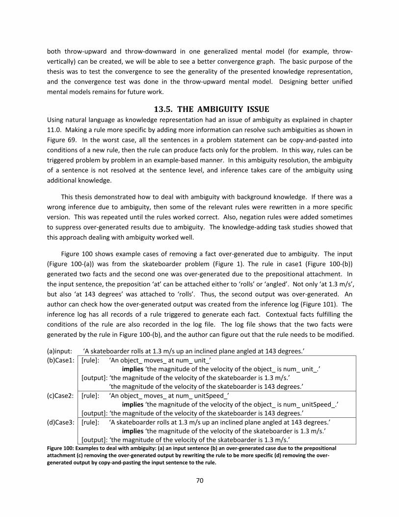
70

both throw-upward and throw-downward in one generalized mental model (for example, throw-

vertically) can be created, we will be able to see a better convergence graph. The basic purpose of the

thesis was to test the convergence to see the generality of the presented knowledge representation,

and the convergence test was done in the throw-upward mental model. Designing better unified

mental models remains for future work.

13.5. THE AMBIGUITY ISSUE Using natural language as knowledge representation had an issue of ambiguity as explained in chapter

11.0. Making a rule more specific by adding more information can resolve such ambiguities as shown in

Figure 69. In the worst case, all the sentences in a problem statement can be copy-and-pasted into

conditions of a new rule, then the rule can produce facts only for the problem. In this way, rules can be

triggered problem by problem in an example-based manner. In this ambiguity resolution, the ambiguity

of a sentence is not resolved at the sentence level, and inference takes care of the ambiguity using

additional knowledge.

This thesis demonstrated how to deal with ambiguity with background knowledge. If there was a

wrong inference due to ambiguity, then some of the relevant rules were rewritten in a more specific

version. This was repeated until the rules worked correct. Also, negation rules were added sometimes

to suppress over-generated results due to ambiguity. The knowledge-adding task studies showed that

this approach dealing with ambiguity worked well.

Figure 100 shows example cases of removing a fact over-generated due to ambiguity. The input

(Figure 100-(a)) was from the skateboarder problem (Figure 1). The rule in case1 (Figure 100-(b))

generated two facts and the second one was over-generated due to the prepositional attachment. In

the input sentence, the preposition ‘at’ can be attached either to ‘rolls’ or ‘angled’. Not only ‘at 1.3 m/s’,

but also ‘at 143 degrees’ was attached to ‘rolls’. Thus, the second output was over-generated. An

author can check how the over-generated output was created from the inference log (Figure 101). The

inference log has all records of a rule triggered to generate each fact. Contextual facts fulfilling the

conditions of the rule are also recorded in the log file. The log file shows that the two facts were

generated by the rule in Figure 100-(b), and the author can figure out that the rule needs to be modified.

(a)input: ‘A skateboarder rolls at 1.3 m/s up an inclined plane angled at 143 degrees.’

(b)Case1: [rule]: ‘An object_ moves_ at num_ unit_’ implies ‘the magnitude of the velocity of the object_ is num_ unit_.’ [output]: ‘the magnitude of the velocity of the skateboarder is 1.3 m/s.’ ‘the magnitude of the velocity of the skateboarder is 143 degrees.’

(c)Case2: [rule]: ‘An object_ moves_ at num_ unitSpeed_’ implies ‘the magnitude of the velocity of the object_ is num_ unitSpeed_.’ [output]: ‘the magnitude of the velocity of the skateboarder is 143 degrees.’

(d)Case3: [rule]: ‘A skateboarder rolls at 1.3 m/s up an inclined plane angled at 143 degrees.’ implies ‘the magnitude of the velocity of the skateboarder is 1.3 m/s.’ [output]: ‘the magnitude of the velocity of the skateboarder is 1.3 m/s.’

Figure 100: Examples to deal with ambiguity: (a) an input sentence (b) an over-generated case due to the prepositional attachment (c) removing the over-generated output by rewriting the rule to be more specific (d) removing the over-generated output by copy-and-pasting the input sentence to the rule.

71

What an author can do now is to rewrite the rule to be more specific so that the rule can be

triggered in a more specific condition. The variable ‘unit_’ was rewritten to ‘unitSpeed_’ in case2 of

Figure 100-(c), and the over-generated output disappeared. What if the over-generated result is still

generated even after all efforts and trials? Even in this worst case, there is still a way to do. Copy-and-

pasting the input sentence to the condition of the rule (case3 of Figure 100-(d)) will make the rule match

the input in only one way as string match. A rule can be rewritten to be used in an example-based

manner in this way. It will sacrifice the generality and reusability of the rule. However it is a good

advantage that there is always a way to remove ambiguities, and there is always a way to make the

system accept an input.

[Inference log]: implied: ‘the magnitude of the velocity of the skateboarder is 1.3 m/s.’ rule: ‘An object_ moves_ at num_ unit_’ implies ‘the magnitude of the velocity of the object_ is num_ unit_.’ ^<--(implied)— ‘A skateboarder rolls at 1.3 m/s up an inclined plane angled at 143 degrees.’ implied: ‘the magnitude of the velocity of the skateboarder is 143 degrees.’ rule: ‘An object_ moves_ at num_ unit_’ implies ‘the magnitude of the velocity of the object_ is num_ unit_.’ ^<--(implied)— ‘A skateboarder rolls at 1.3 m/s up an inclined plane angled at 143 degrees.’ … Figure 101: Inference log of the case1 of Figure 100

13.6. THE OVER-GENERATION ISSUE One of the concerns raised by using both generalized and specific knowledge was that multiple rules can

be triggered by a fact. Authors usually enter a specific version of knowledge, and the system can

generalize knowledge, or authors can enter generalized knowledge directly. In such cases, multiple rules

can be triggered. Knowledge subsumption was introduced to find the most specific rule to trigger

(chapter 10.3) , and it fixed most over-generated ouputs. However there are still possible cases of over-

generation. It is possible that an input sentence can trigger two rules and they cannot be arranged

based on subsumption relations even when only one of them should be triggered.

Input: ‘what is the vertical velocity of the ball?’

Rules: ‘what is vector__?’ implies ‘what is the magnitude of vector__?’ ‘what is the vertical vector__?’ implies ‘what is the y-component of the vector__?’

Output: ‘what is the magnitude of the vertical velocity of the ball?’ (x) ‘what is the y-component of the velocity of the ball?’ (o) Figure 102: over-generation example

In Figure 102, the input ‘what is the vertical velocity of the ball?’ will trigger the two rules. The

condition of the second rule is more specific, but a subsumption relation is not found in them because of

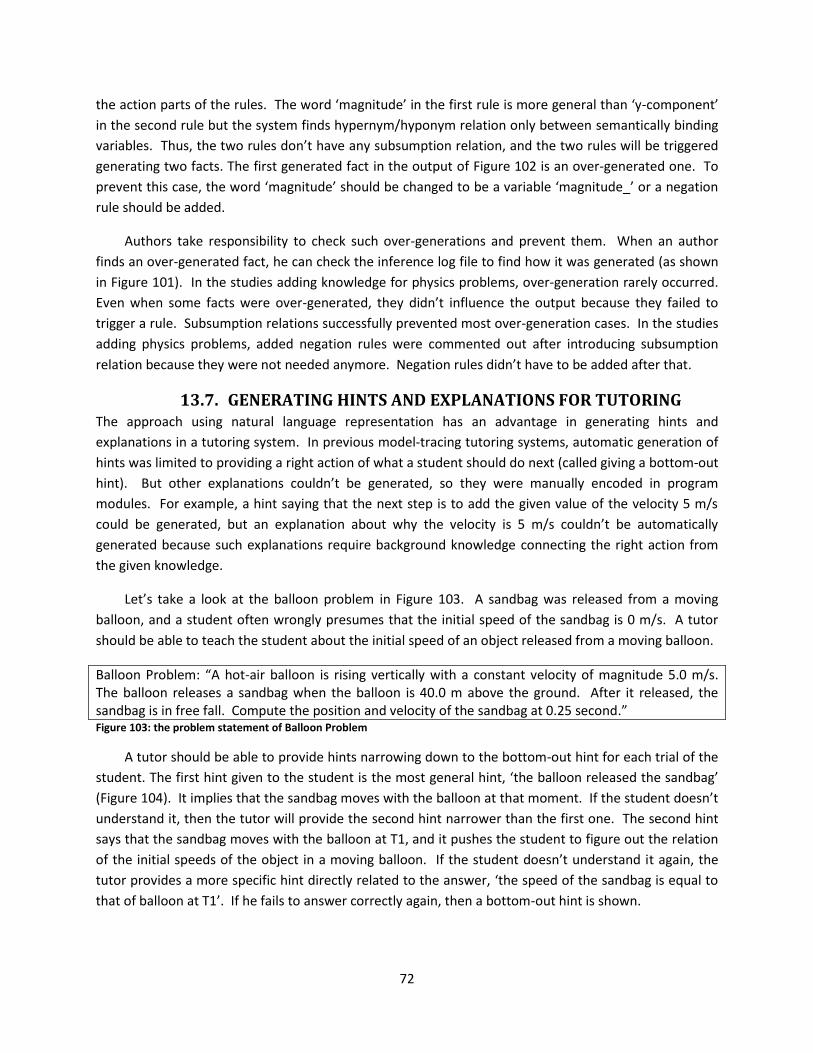
72

the action parts of the rules. The word ‘magnitude’ in the first rule is more general than ‘y-component’

in the second rule but the system finds hypernym/hyponym relation only between semantically binding

variables. Thus, the two rules don’t have any subsumption relation, and the two rules will be triggered

generating two facts. The first generated fact in the output of Figure 102 is an over-generated one. To

prevent this case, the word ‘magnitude’ should be changed to be a variable ‘magnitude_’ or a negation

rule should be added.

Authors take responsibility to check such over-generations and prevent them. When an author

finds an over-generated fact, he can check the inference log file to find how it was generated (as shown

in Figure 101). In the studies adding knowledge for physics problems, over-generation rarely occurred.

Even when some facts were over-generated, they didn’t influence the output because they failed to

trigger a rule. Subsumption relations successfully prevented most over-generation cases. In the studies

adding physics problems, added negation rules were commented out after introducing subsumption

relation because they were not needed anymore. Negation rules didn’t have to be added after that.

13.7. GENERATING HINTS AND EXPLANATIONS FOR TUTORING The approach using natural language representation has an advantage in generating hints and

explanations in a tutoring system. In previous model-tracing tutoring systems, automatic generation of

hints was limited to providing a right action of what a student should do next (called giving a bottom-out

hint). But other explanations couldn’t be generated, so they were manually encoded in program

modules. For example, a hint saying that the next step is to add the given value of the velocity 5 m/s

could be generated, but an explanation about why the velocity is 5 m/s couldn’t be automatically

generated because such explanations require background knowledge connecting the right action from

the given knowledge.

Let’s take a look at the balloon problem in Figure 103. A sandbag was released from a moving

balloon, and a student often wrongly presumes that the initial speed of the sandbag is 0 m/s. A tutor

should be able to teach the student about the initial speed of an object released from a moving balloon.

Balloon Problem: “A hot-air balloon is rising vertically with a constant velocity of magnitude 5.0 m/s. The balloon releases a sandbag when the balloon is 40.0 m above the ground. After it released, the sandbag is in free fall. Compute the position and velocity of the sandbag at 0.25 second.” Figure 103: the problem statement of Balloon Problem

A tutor should be able to provide hints narrowing down to the bottom-out hint for each trial of the

student. The first hint given to the student is the most general hint, ‘the balloon released the sandbag’

(Figure 104). It implies that the sandbag moves with the balloon at that moment. If the student doesn’t

understand it, then the tutor will provide the second hint narrower than the first one. The second hint

says that the sandbag moves with the balloon at T1, and it pushes the student to figure out the relation

of the initial speeds of the object in a moving balloon. If the student doesn’t understand it again, the

tutor provides a more specific hint directly related to the answer, ‘the speed of the sandbag is equal to

that of balloon at T1’. If he fails to answer correctly again, then a bottom-out hint is shown.

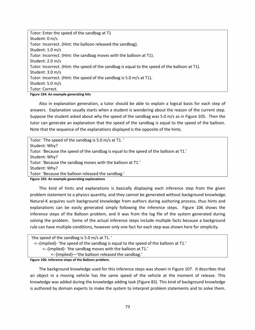
73

Tutor: Enter the speed of the sandbag at T1 Student: 0 m/s Tutor: Incorrect. (Hint: the balloon released the sandbag). Student: 1.0 m/s Tutor: Incorrect. (Hint: the sandbag moves with the balloon at T1). Student: 2.0 m/s Tutor: Incorrect. (Hint: the speed of the sandbag is equal to the speed of the balloon at T1). Student: 3.0 m/s Tutor: Incorrect. (Hint: the speed of the sandbag is 5.0 m/s at T1). Student: 5.0 m/s Tutor: Correct. Figure 104: An example generating hits

Also in explanation generation, a tutor should be able to explain a logical basis for each step of

answers. Explanation usually starts when a student is wondering about the reason of the current step.

Suppose the student asked about why the speed of the sandbag was 5.0 m/s as in Figure 105. Then the

tutor can generate an explanation that the speed of the sandbag is equal to the speed of the balloon.

Note that the sequence of the explanations displayed is the opposite of the hints.

Tutor: ‘The speed of the sandbag is 5.0 m/s at T1. ’ Student: Why? Tutor: ‘Because the speed of the sandbag is equal to the speed of the balloon at T1.’ Student: Why? Tutor: ‘Because the sandbag moves with the balloon at T1.’ Student: Why? Tutor: ‘Because the balloon released the sandbag.’ Figure 105: An example generating explanations

This kind of hints and explanations is basically displaying each inference step from the given

problem statement to a physics quantity, and they cannot be generated without background knowledge.

Natural-K acquires such background knowledge from authors during authoring process, thus hints and

explanations can be easily generated simply following the inference steps. Figure 106 shows the

inference steps of the Balloon problem, and it was from the log file of the system generated during

solving the problem. Some of the actual inference steps include multiple facts because a background

rule can have multiple conditions, however only one fact for each step was shown here for simplicity.

‘the speed of the sandbag is 5.0 m/s at T1. ’ <--(implied)- ‘the speed of the sandbag is equal to the speed of the balloon at T1.’ <--(implied)- ‘the sandbag moves with the balloon at T1.’ <--(implied)—‘the balloon released the sandbag.’ Figure 106: inference steps of the Balloon problem.

The background knowledge used for this inference steps was shown in Figure 107. It describes that

an object in a moving vehicle has the same speed of the vehicle at the moment of release. This

knowledge was added during the knowledge adding task (Figure 83). This kind of background knowledge

is authored by domain experts to make the system to interpret problem statements and to solve them.

74

Thus, the background knowledge for problem solving can be used to generate hints and explanations,

and no extra process is needed to acquire such knowledge for generating hints and explanations.

‘A vehicle_ moves_ vertically with a velocity of magnitude num_ unit_’ and implies ‘the vehicle_ moves_ vertically at T_’ and ‘the speed of the vehicle_ is num_ unit_ at T_’. ‘A vehicle_ releases an object_’ and ‘the vehicle_ moves at T_’ imply ‘the object_ moves with the vehicle_ at T_’. ‘An object_ moves with an vehicle_ at T_’ and implies ‘the speed of the object_ is equal to the speed of the vehicle_ at T_’. ‘The speed of an object_ is equal to the speed of a vehicle_ at T_’ and ‘the speed of the vehicle_ is num_ unit_ at T_’ imply ‘the speed of the vehicle_ is num_ unit_ at T_’. Figure 107: background knowledge for the balloon example

A similar approach is often used in the expert systems field, where a user asks an expert system to

explain its reasoning (Swartout, Paris, & Moore, 1991 ) (Eugenio, Fossati, Yu, Haller, & Glass, 2005),

although generating explanations is still limited without such background knowledge. After the system

has isolated the reasoning that led up to the assertion being questions, that formal chain of reasoning is

converted into natural language. This is a challenging natural language generation problem that is

obviated by having the reasoning itself represented in natural language.

13.8. A NEW KIND OF INTELLIGENT TUTORING SYSTEMS The tutoring systems in this section are suggestion of a novel kind of tutoring systems which were not

built or tested.

13.8.1. An ITS for Problem Understanding

As mention before, using unconstrained natural language as knowledge representation enabled Natural-

K to acquire knowledge connecting input sentences and principles which is missing in current physics

tutors. As shown in section 13.7, this kind of knowledge is required in understanding a problem before

actual problem solving procedure. For example in the Balloon Problem (Figure 103), a student reads the

statement line by line and tries to find a mapping to a relevant mental model. This student behavior is

about understanding the problem. The knowledge about the initial velocity in a moving vehicle (in

Figure 107) is part of the knowledge for understanding the problem before starting to solve it. This type

of knowledge was not used before for tutoring. Previous physics tutors had to mainly focus on the

tutoring assigning known values to variables and applying principles rather than tutoring how to

understand the problem.

Thus, using the new type of knowledge, a new kind of ITS can be designed mainly focusing on

tutoring problem understanding. For example, in the Balloon Problem, instead of using for hints and

explanations, the background knowledge can be treated as part of solution path the student should

75

follow. As shown in Figure 108, the inference steps in Figure 106 is part of a solution that the student

should answer. A shortcut can be used to jump inference steps in case the student already understands

everything. For example, he can directly enter the speed of the sandbag at the first question. The

remaining part of tutoring can be same to the previous physics tutoring. Extra modules are needed to

recognize the student input in natural language.

Tutor: What can you infer from the first sentence of the problem statement? Student: hm, I don’t know. Tutor: You can infer the speed of the sandbag at T1 Student: The speed of the sandbag is equal to the speed of the balloon at T1. Tutor: Good, then? Student: The speed of the sandbag is 5.0 m/s. Tutor: Great. Figure 108: An example of an ITS helping a student how to understand the Balloon problem (Figure 103).

13.8.2. A Teachable Agent

Instead of instructors, students can add problems to an ITS If the authoring task is easy enough for

students can do. Knowledge is represented in natural language, so there is no big theoretical barrier for

this. This section suggests a simplified version using graphical user interface.

Figure 109 shows how a student can add the skateboarder problem (Figure 1) to the system.

Before start, he reads the problem statement to understand the given problem. First, he draws an

object. Second, he enters the object name. Third, he draws a vector. Fourth, he enters the magnitude

of the velocity in natural language. Fifth, he enters the direction of the velocity in natural language.

Sixth, he enters a question. Seventh, he enters principles in natural language. Eighth, the system solves

it displaying an answer.

76

skateboarder

The magnitude of the velocity of the skateboarder is 3 m/s

The direction of the velocity of the skateboarder is 30 degrees

What is the y-component of the velocity of the skateboarder?

x=mag*cos(theta)y=mag*sin(theta)where mag is the magnitude of the vector of an object

and theta is the direction of the vector of the objectand x is the x-component of the vector of the objectand y is the y-component of the vector of the object.

1

2

3

4

5

6

7

8 the y-component of the velocity of the skateboarder is 1.5 m/s

Figure 109: the process of student’s adding the skateboarder problem to the system.

If the solution by the system is not correct, the student has to figure out what is wrong, and to fix it.

He needs to repeats this task until the system can solve the problem correctly. It is a process that the

student teaches the system, and he can learn by teaching the system. The system can be switched to a

tutoring mode, and the added problem can be used to teach other students after polishing. Then, it can

be called learning by authoring.

13.8.3. Application to the Law Domain

All levels of knowledge were separated from program code, and knowledge was represented in

unconstrained natural language. Thus, this approach can be applied to any other domains where

knowledge can be represented in natural language. For example in the law domain, articles listed in a

law book (Figure 110-(a)) can be authored as rules in natural language as Figure 110-(b):

(a) ‘If a defendant murdered a victim, then he should receive imprisonment for life.‘

(b) ‘A defendant murdered a victim’ implies ‘he should receive imprisonment for life‘

Figure 110: An example of an article (a) in a law book (b) in a form of rule

A bill of indictment in the law domain corresponds to a problem statement in physics:

“The name of the defendant is Mr. John Gold. The defendant shot at the victim July 24 in the victim’s house.

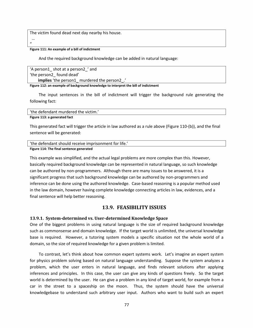
77

The victim found dead next day nearby his house. …

“ Figure 111: An example of a bill of indictment

And the required background knowledge can be added in natural language:

‘A person1_ shot at a person2_’ and ‘the person2_ found dead’ implies ‘the person1_ murdered the person2_.’ Figure 112: an example of background knowledge to interpret the bill of indictment

The input sentences in the bill of indictment will trigger the background rule generating the

following fact:

‘the defendant murdered the victim.’ Figure 113: a generated fact

This generated fact will trigger the article in law authored as a rule above (Figure 110-(b)), and the final

sentence will be generated:

‘the defendant should receive imprisonment for life.’ Figure 114: The final sentence generated

This example was simplified, and the actual legal problems are more complex than this. However,

basically required background knowledge can be represented in natural language, so such knowledge

can be authored by non-programmers. Although there are many issues to be answered, it is a

significant progress that such background knowledge can be authored by non-programmers and

inference can be done using the authored knowledge. Case-based reasoning is a popular method used

in the law domain, however having complete knowledge connecting articles in law, evidences, and a

final sentence will help better reasoning.

13.9. FEASIBILITY ISSUES

13.9.1. System-determined vs. User-determined Knowledge Space

One of the biggest problems in using natural language is the size of required background knowledge

such as commonsense and domain knowledge. If the target world is unlimited, the universal knowledge

base is required. However, a tutoring system models a specific situation not the whole world of a

domain, so the size of required knowledge for a given problem is limited.

To contrast, let’s think about how common expert systems work. Let’s imagine an expert system

for physics problem solving based on natural language understanding. Suppose the system analyzes a

problem, which the user enters in natural language, and finds relevant solutions after applying

inferences and principles. In this case, the user can give any kinds of questions freely. So the target

world is determined by the user. He can give a problem in any kind of target world, for example from a

car in the street to a spaceship on the moon. Thus, the system should have the universal

knowledgebase to understand such arbitrary user input. Authors who want to build such an expert

78

system should add almost an infinite amount of world knowledge to make the system ready to

understand any natural language input. This is one of the reasons why the idea of applying natural

language understanding was not successful in general AI domains.

Now, let’s think about a tutoring system to see the difference. Let’s assume that you are building a

tutoring system for a physics domain. Now, the system gives a physics problem, and a student should

solve it. Thus, the student experiences only the predefined situation in the problem given by the system.

It makes the size of the required background knowledge limited. It is enough to add domain problems

one by one in the authoring task. Moreover, the student is not supposed to do anything other than

solving the given problems. The given physics problem determines the system behaviors (or the

solution path), and the system determines the correct student behaviors. Student behaviors outside the

solution path can easily be treated as wrong or simply ignored. Thus, the required knowledge is

determined by the solution path which is generated by the given physics problem. The size of the

knowledge is proportional to the number of relevant principles and their variables. The number of

relevant principles is also limited so that the student can solve a given problem in a short amount of

time. These restrictions together make the target world of the systems small enough to apply natural

language understanding for authoring task. These restrictions are from the characteristics of a tutoring

system.

It is worth clarifying what types of AI applications have a similar property like tutoring systems.

Let’s categorize all AI applications into two types. The first is applications in which the expected user

behaviors are determined by a system. The applications in this type have a system-determined

knowledge space. In applications in this type, the size of the background knowledge is usually small

enough to be added by authors. For example, game programming has such a property. The way of

playing the game, assigning scores, surviving and death conditions are all determined by the game

program. Game players are supposed to get scores playing the game following a predetermined survival

path. Note that a tutoring system has similar aspects to a game program providing high scores to

students who are good at solving problems. If the applications are generalized further, programming in

natural language can be regarded as the ultimate application in this type. Basically, programming is a

kind of authoring task to write fixed algorithms usually running without user input. Thus, a programmer

doesn’t have to worry about adding knowledge for user input in this case.

The second type of applications has the property that the expected system behaviors are

determined by a user. Question answering systems such as the web search service, and a

conversational agent have such a property. A system in this type is supposed to respond to a question

asked by a user. Expected answers are determined based on what a user asked. The size of required

background knowledge is almost unlimited because the system doesn’t know what the user will ask.

The set of questions asked by users can change drastically depending on users. The applications in this

type have a user-determined knowledge space. A conversational agent which can pass the Turing test

showing dialogue ability undistinguishable from humans can be the ultimate application in this type.

79

13.9.2. The Issue of Commonsense Knowledge

It was generally believed that a computer system couldn’t do human-like inference because a computer

didn’t have commonsense knowledge. Several attempts were made to build commonsense

knowledgebase (OpenCyc Tutorial) (Chklovski, 2003) (Speer, 2007) (Dolan & Richardson, 1996)

(Harabagiu & Moldovan, 1994) but it is unlikely to see the complete and universal commonsense

knowledgebase containing all human knowledge in the near future. Such approaches to build universal

knowledgebase treated commonsense knowledgebase as a dictionary that can be built once and

updated with small maintenance costs.

There are issues in such dictionary-based approaches of commonsense knowledge. Firstly, the

scope of commonsense knowledge is not clear. For example, gravity acting on an object near a planet,

and buoyancy acting on an object in water belong to commonsense to many people, but not necessarily

to everyone. Still there are many people who don’t know about the concept of buoyancy, so it is not

clear whether this knowledge should be in the commonsense knowledgebase. There are many other

concepts such as electric forces, quantum forces, and there is no clear criteria to determine exactly what

knowledge should be in the commonsense knowledgebase. Most knowledge from the commonsense

knowledgebase currently being built is not required in physics solving task, and most required

knowledge in physics domain is not found in the commonsense knowledgebase.

Secondly, a commonsense knowledge base builder doesn’t know exactly what knowledge is

required in a specific task in many different domains. For example in the skateboarder problem (Figure

1), it is obvious for humans that the velocity of the skateboarder is 1.3 m/s, and humans even may not

realize underlying knowledge working on the recognition process. The knowledgebase builder may not

know that the background knowledge shown in Figure 8 is required in physics solving. The required

background knowledge is dependent on task, and the same background knowledge may not be required

in other tasks. The background knowledge not belonging to commonsense still needs be added

individually depending on tasks and domains.

Lastly, commonsense knowledge was represented in formal language. Thus, only trained users,

preferably with a programming background, can build such knowledge. Using graph representation

(Gunning & Chaudhri, 2010) (Chaudhri, John, Mishra, Pacheco, Porter, & Spaulding, 2007)(Clark, et al.,

2001) is basically not different from using formal language in that users have to be educated to learn the

graph representation. Moreover, the transformation method has to be used if natural language input is

given, and it ends up encountering the issue that only programmers can update the transformation

knowledge.

In the ultimate solution, commonsense knowledge acquisition should be done in a similar way to

how a human acquires knowledge. Basically, a human acquires knowledge in natural language. Natural-

K acquires knowledge in natural language too in a similar way. As explained in the previous section, a

tutoring system is the type of application with a system-determined knowledge space. Thus, the size of

required knowledge to add is small enough to be added by an author. The graphs from the studies

showed that the average number of rules was 10.3 at the first set (Figure 82), 4.5 at the second set

(Figure 83), and it converged to near zero at the third set (Figure 84).

80

13.9.3. The Issue of Paraphrases

One of the problems in the natural language representation is that there can be a large number of

different expressions for a sentence. When knowledge is represented in natural language, there can be

millions of different expressions for it. A system should recognize them as different expressions with the

same meaning. It is unreasonable to expect that authors can add them all. This is called the paraphrase

problem. Following is an example of different expressions with the same meaning.

“An old plane takes off.” “There is an old plane that takes off.” “A old plane starts to fly.” “It is known that an old plane takes off” …

Figure 115: examples of paraphrase

However, an ITS only needs to understand the sentences that appear in a problem statement. If a

particular sentence is not understood, the author can add a rule for the paraphrase or reword it. This

was evaluated in the authoring test, described earlier.

However, the system was designed to generalize knowledge to extend the scope of acceptable

input patterns. As more knowledge is added, and as the system has more generalized knowledge, the

system will be able to recognize increasingly more different expressions. Initially an author should add

all required knowledge, but the amount of knowledge to be added will decrease as he adds more

knowledge converging to zero ultimately (Figure 97). At the study of knowledge adding task in a throw-

upward mental model, the number of added rules converged fast (Figure 84).

The paraphrase problem can rise seriously in the second type of applications with user-determined

knowledge space. For example, if the system is supposed to answer physics questions asked by a user,

the system should have the complete and universal knowledgebase to understand all paraphrases

thrown by the user. Without such a universal knowledgebase, recognizing paraphrases becomes a

serious issue in this type of applications.

13.10. WHAT IS NEW IN THE THESIS? The goal of this thesis was to build an authoring system allowing authors to add not only physics

problems, but also background knowledge in natural language. Prior to this thesis, it was not known

whether using natural language rules and principles would work. The thesis concentrated on developing

methods for authoring background knowledge, including principles. Many new ideas and approaches

were proposed in this thesis, however only the main ideas are listed as follows.

The first idea introduced here is background rules represented in natural language (Figure 8-(a)).

Implication rules and truth rules were introduced, and they have natural language in left and right sides

(i.e. conditions, actions, and hypotheses). Natural language is used both for conditions and actions in

the rules. This idea enables non-programmers to read and write background knowledge easily. Without

this idea, inference would have to be done in formal language and the problem statements would need

transformation into formal language. Transformation approach was a common way in previous studies,

81

but required background knowledge had to be encoded in program codes that can be updated only by

computer programmers.

The second idea is to let authors to add background knowledge. Recently several attempts are

being made to build the universal commonsense knowledge base. However, building such knowledge

base may not be completed soon (if “completion” even makes sense for them), so this approach was not

adopted. It seems more natural for a system to acquire background knowledge from authors in natural

language.

The third idea is to represent principles in natural language. In previous studies, principles had to

be encoded in computer program codes, and it became the reason why knowledge was not completely

separated from program codes. By representing principles in natural language, all types of knowledge

were separated from program codes. It made the inference process transparent as shown in Figure 9,

and it made possible for non-programmers to read and understand the intermediate inference steps

directly.

The fourth idea is the generalized natural language representation using semantically binding

variables (Figure 8-(b), and Chapter 7.0). The generalized representation was used to accept broad

range of input patterns, and it is readable for non-programmers because it is still natural language.

Semantically binding phrase variables were introduced to maximize the idea of generalized natural

language representation.

The fifth idea is to use unconstrained natural language as knowledge representation. The core

mechanism used in inference is simply matching two sentences from input and a rule. The system

doesn’t have any predefined sentence patterns, templates, or transformation knowledge encoded in

program code or grammar except a few variables (Figure 22). It simply matches an input sentence and a

condition from a rule, and both are in natural language. Thus, there is no need to impose constraints on

natural language, and there is no place where non-programmers cannot update domain knowledge.

Representing background knowledge in a form of rule, and using semantically binding variables for

generalized representation made it possible to use unconstrained natural language as knowledge

representation. Even an ungrammatical sentence can be accepted if a condition of a rule has the same

sentence to the input although not desirable in this application.

The sixth idea is default knowledge represented in natural language. Some knowledge is given by

default if not mentioned in a given problem. Such knowledge was represented in the same framework

of natural language representation.

The seventh idea is representation of time using time variables. Before this thesis began, such

problems with handling time were not anticipated, and quite a lot of efforts had to be made for them.

Discovering and solving the problem of explicating time is one of the contributions of the thesis.

Symbolic representation of time was used to designate the location on a problem statement. Time of an

event was indexed pointing to a verb in a sentence. Time indexes were sorted to arrange events in the

time domain. Using a phrase variable to recognize time phrase (Figure 34) was introduced.

82

The eighth idea is mental model extensions. Some physics mental model share a basic mental

model. The idea of mental model extension was introduced to reuse an existing basic mental model.

13.11. WHY HASN’T IT BEEN DONE BEFORE? Using natural language for knowledge acquisition and to represent knowledge was an old dream in the

Artificial Intelligence area. Some attempts were made going toward this direction. In the ITS and

problem solving area, such attempts were done until 1970s (Bobrow, 1964) (Novak Jr., 1977) (Bundy,

Byrd, Luger, Mellish, & Palmer, 1979), but the area has been inactive since then.

The biggest problem was background knowledge. The idea of using natural language doesn’t work

without commonsense knowledge. Because a commonsense knowledgebase was not available, the

previous studies were limited in transforming restricted input patterns, and they were not able to go

further. This bottleneck was common in the AI area.

After the recognition of the bottleneck, new attempts started to build commonsense

knowledgebase after 1990s (Chklovski, 2003) (Speer, 2007) (Dolan & Richardson, 1996) (Harabagiu &

Moldovan, 1994). But their goal was to build the universal commonsense knowledge that can be used in

general AI problems such as question answering. A problem of this approach is that most applications

will not work until they build the complete commonsense knowledgebase and this goal is still distant.

Even a human doesn’t have such universal commonsense knowledge. Human commonsense is different

from a person to person, from a nation to nation, and from a culture to culture. A human keeps learning

new background knowledge and updating his commonsense knowledge. Project Halo used graphical

notation to represent domain knowledge and authors were asked to add knowledge (Gunning &

Chaudhri, 2010). However the graphical representation is still formal language that authors should be

trained to use it. Also it is inevitable to adopt the transformation approach to receive natural language

input if such formal representation (or graphical representation) is used.

It became the motivation of this thesis to find a way to acquire background knowledge including

commonsense from humans. But such a goal was not attainable until realizing the new idea

representing knowledge in unconstrained free natural language. A bunch of new ideas and new

approaches had to be created to make this breakthrough, such as representing various types of

knowledge (implication rules, truth rules, default knowledge, principles, etc.) in natural language, and

generalized representation using the semantically binding variables. Representing principles in natural

language completely separated the knowledge level from the programming level, and it made possible

to use unconstrained natural language as knowledge representation.

Another reason why it hasn’t been done before is due to the difference of tutoring systems from

other AI systems that a user determines expected system behaviors. Even if all the ideas work fine,

there is still a problem in such type of AI applications with user-determined knowledge space. Many AI

systems generally work responding to the user. A user asks a question, then the AI systems try to find

answers responding properly. The correct system behaviors and required knowledge space are

determined by what the user asks. When the AI system cannot constrain what the user will say, then

the required background knowledge becomes almost unlimited. The previous AI applications mainly

83

were from question-answering systems and human-computer interactions with user-determined

knowledge space.

On the other hand, a tutoring system leads the interaction and thus determines correct behaviors

of the student. An ITS gives a problem, then a student should solve it. The system knows how the

student should respond, and it focuses on generating correct solutions and comparing them to student

responses. The size of background knowledge is determined by the system and directly by the given

problem. Thus, the related amount of background knowledge is limited on the problem. Authoring task

using natural language is feasible in this type of applications with system-determined knowledge space.

Due to this interesting property, this approach representing knowledge in natural language and

acquiring from humans couldn’t be done in other AI domains.

13.12. FUTURE WORK

13.12.1. Rule generalization

The rule generalization process was not implemented yet because the generalized rules were

represented in natural language and an author was able to add them directly. Instead of expecting

authors to add generalized rules, authors can add the most specific rules, and the system in the future

can create generalized rules based on what authors added.

If authors have to add generalized knowledge, they take responsibility of regression test of the

knowledgebase. In the regression test, they have to check all previous problems whenever they modify

the knowledgebase. The system can inform authors if there is a change of output of the previous

problems. However, authors have to maintain the knowledgebase so that all previous problems to be

solved correctly. This is a painful task for authors. By letting authors add the most specific examples,

the system takes responsibility for regression testing the knowledgebase. The system should be able to

produce generalized rules not influencing previously solved problems.

Rule generalization can be done in two ways. One way is to make a sentence shorter removing

words to make more specific. It is a property of natural language that a longer sentence usually has a

more specific meaning. By making a sentence shorter, the meaning can be generalized. The other way

is to replace a word with a semantically binding variable with a broader meaning. A condition of a rule

can be generalized by replacing a word with its hypernym word. The system can create generalized

rules covering multiple specific rules added by authors in this way.

13.12.2. More Natural Representation

The proposed semantically binding variables have an underbar at the right side. Is it possible to use

them without an underbar to make it a perfect natural language sentence? Yes, it is possible. But there

are examples with complications in matching and assignment. Figure 116 shows such an example with

an underbar (upper) and without an underbar (lower). But, the representation without an underbar

doesn’t designate exactly which ones are variables, so all the words are possible variables. The right

side of the first example, it is clear that only the first object_ is a variable. But in the right side of the

second example, it is not easy to know which one is a variable among the two words object (i.e. ‘the

object’ and ‘a physics object’). It makes the matching algorithm and the rule generalization process

84

complicated. During matching process it will increase computational costs too. It is an issue how to

design an efficient matching algorithm. It remains as future work.

‘An agent_ moves_ an object_’ implies ‘the object_ is a physical object’.

‘‘An agent moves an object’ implies ‘the object is a physical object’.

Figure 116: semantically binding variables with an underbar (upper) and without an underbar (lower)

13.12.3. Where Can We Go Further?

For the first time, knowledge represented in unconstrained natural language was used from the input

through the whole inference process. The knowledge level was completely separated from the

programming level, and knowledge was freed from restrictions imposed by programming code. Where

can we go further with this breakthrough? What is the ultimate place to go along with this direction?

In intelligent tutoring systems, a tutoring system with an empty knowledgebase can be given to a

student. The student can teach the empty tutor by adding knowledge, and he learns problem solving

during authoring the system. It is similar to a learning-by-teaching approach (Schwartz, et al.,

2009)(Chen, Liao, & Chan, 2010). In the current learning-by-teaching approach, the applicable domain

was limited because it was not imaginable for students to add knowledge in formal language to the

system. Only fixed and predefined simple forms of knowledge were used for teaching such as Boolean

relations.

In the natural language based approach, students can teach the system by adding knowledge in

natural language. They can check the intermediate inference done by the system, and fix knowledge if

necessary. Through this authoring task, students can acquire deep understanding of problem solving. It

can be called learning-by-authoring approach in a point that the students can teach the system up to the

level where the system can teach other students. The level of expertise the student can acquire is

higher, and the required level of understanding is deeper than learning-by-teaching. Ideally speaking,

the system with an empty knowledgebase can be distributed to students, and students can learn by

authoring the system adding knowledge. Some excellent students will be able to build a nice

knowledgebase, and it can be used to teach other students after polishing up by a teacher. In this way,

the tutoring system can be distributed in many domains with empty knowledgebase in an ultimate stage.

In the natural language understanding area, Natural-K corresponds to the realization of language

understanding using knowledge represented in natural language. In previous studies, natural language

was regarded as understood when it was interpreted in formal language. In the approach using natural

language representation, natural language was regarded as understood when it was properly

interpreted in knowledge represented in natural language and the knowledge was correctly used to

perform tasks. By applying the idea of learning-by-authoring, it is possible to build an intelligent agent

or a humanoid robot performing tasks defined by a user who is not a programmer. For example, a user

can teach the agent to filter out spam mails by adding knowledge about detecting spam mails in natural

language. In case of a humanoid robot application, a human can teach a robot a new task such as

cleaning up a dinner table in natural language telling how to clean and when to clean it.

85

In general in the artificial intelligence area, if we go further in this direction with the idea of using

natural language to represent knowledge, we will meet one of the old AI problems, programming in

natural language. Natural-K is not far from there. Most concepts required in basic computer

programming were already introduced in Natural-K. The problem statement is a kind of program code

interpreted line by line. A background rule is a kind of function with conditions, and the problem

statement will trigger it. Semantically binding variables in the conditions are arguments passing by a

function call. The action part of the rule is a kind of program code inside a function. Each line of the

actions is interpreted triggering other rules like each line of a function code can trigger other function.

The context memory is a kind of global memory. The issues about how to implement loops, conditionals,

and local variables remain to go toward programming in natural language.

CONCLUSIONS Using natural language as knowledge representation is a significant shift of idea in knowledge

representation in that the computer system can perform human-like-inference using the same type of

knowledge readable both to humans and computers.

The main idea in this thesis was to use unconstrained natural language to represent knowledge in

an ITS so that the system can understand a problem statement directly, and non-programmers can add

required knowledge. In the authoring task studies, the physics problems in kinematics, statics, and

dynamics problems were added and solved successfully. The problems in one mental model (throw-

upward) showed that the system entered the no-new-knowledge state fast and the number of added

rules converged to near zero. The recruited subjects were able to add the problems in the no-new-

knowledge state either by rewording or adding knowledge. The studies showed that the number of

required new rules was small enough for an author to add, and that the generalized representation was

effective in reusing existing knowledge helping fast convergence.

This result suggests that the system can be given to domain experts after an initial knowledgebase

was built by knowledge engineers. The system entered the no-new-knowledge state after ten problems

in the throw-update mental model. More than one third of the problems in the state were solved

automatically without adding a new rule. It is expected that increasingly more problems can be solved

as more problems are added.

The basic idea of using natural language as knowledge representation may have other applications

besides ITS authoring. A tutoring system has an interesting property that the expected student

behaviors are determined by the system not by a user, and the size of required knowledge is limited. It

suggests that the natural language approach can be applied to other AI application where expected user

behaviors are determined by a system rather than users.

The presented system acquires knowledge from humans in natural language, and performs

inference in natural language similarly to the way a human does. It is a significant breakthrough going

toward the traditional idea of AI, i.e. human-like inference. It will pave a way to go to learning-by-

authoring in ITS, and further toward programming in natural language.

86

BIBLIOGRAPHY Aleven, V., & Bruce M. McLaren, J. S. (2009). A New Paradigm for Intelligent Tutoring Systems: Example-

Tracing Tutors. (J. Lester, Ed.) International Jounal of Artificial Intelligence in Eudcation , 19, 105-164.

Amstutz, D. (2001). General Physics: Pearls of Wisdom. Jones & Bartlett Learning.

Blatt, F. J. (1989). Principles of Physics (third edition ed.). Allyn and Bacon.

Bobrow, D. G. (1964). Natural Language Input for a Computer Problem Solving System. Ph. D. Thesis,

Massachusetts Institute of Technology, Cambridge, MA, USA .

Brachman, R. J., & Levesque, H. J. (2004). Knowledge Representation and Reasoning. Morgan Kaufmann.

Bundy, A., Byrd, L., Luger, G., Mellish, C., & Palmer, M. (1979). Solving mechanics problems using meta-

level inference. 6th International Joint Conference on Artificial Intelligence (pp. pp. 1017-1027). Tokyo:

William Kaufmann.

Chaudhri, V. K., John, B. E., Mishra, S., Pacheco, J., Porter, B., & Spaulding, A. (2007). Enabling experts to

build knowledge bases from science textbooks. International Conference On Knowledge Capture, (pp.

pp.159 - 166).

Chen, Z.-H., Liao, C., & Chan, T.-W. (2010). Learning by Pet-training Competition: Alleviating Negative

Influences of Direction Competition by Training Pets to Compete in Game-Based Environments. 10th

IEEE International Conference on Advanced Learning Technologies, (pp. 411 - 413 ). Sousse, Tunesia.

Chi, M., & VanLehn, K. (2008). Eliminating the Gap between the High and Low Students through Meta-

Cognitive Strategy Instruction. 9th International Conference of Intelligent Tutoring Systems (pp. pp 603-

613). Amsterdam: IOS Press.

Chi, M., & VanLehn, K. (2007). The impact of explicit strategy instruction on problem-solving behaviros

across intelligent tutoring systems. Proceedings of the 29th Annual Conference of the Cognitive Science

Society, (pp. pp. 167-172). NJ: Erlbaum.

Chklovski, T. (2003). Learner: a system for acquiring commonsense knowledge by analogy., (p.

Knowledge Capture).

Clark, P., Thompson, J., Barker, K., Porter, B., Chaudhri, V., Rodriguez, A., et al. (2001). Knowledge entry

as the graphical assembly of components. International Conference On Knowledge Capture, (pp. pp. 22-

29).

Crowell, B. (2000). Newtonian Physics. Light and Matter.

David Gunning, V. K. (2010). Project Halo Update - Progress Toward Digital Aristotle. AI Magazine , 31 (3),

33-58.

87

De Kleer, J. (1975). Qualitative and quantitative knowledge in classical mechanics. MIT AI Laboratory,

Cambridge, MA.

Dolan, W. B., & Richardson, S. D. (1996). Not for its own sake: knowledge as a byproduct of natural

language processing. AAAI Technical Report FS-96-04. AAAI.

Eugenio, B. D., Fossati, D., Yu, D., Haller, S., & Glass, M. (2005). Natural Language Generation for

Intelligent Tutoring Systems: a case study. the 12th International Conference on Artificial Intelligence in

Education. Amsterdam, Netherlands.

Ewen, D., Nelson, R. J., & Schurter, N. (1996). Physics for career education (fifth edition ed.). Prentice-

Hall.

Fellbaum, C. (1998). WordNet: An Electronic Lexical Database. Cambridge, MA: MIT Press.

Fogiel, M. (1976 ). The physics problem solver. (J. J. Molitoris, Ed.) Research and Education Association.

Fuchs, N. E., Kaljurand, K., & Kuhn, T. (2008). Attempto Controlled English for Knowledge Representation.

Reasoning Web, 4th Intern'l Summer School, (pp. pp. 104-124).

Gunning, D., & Chaudhri, V. K. (2010). Project Halo Update - Progress Toward Digital Aristotle. (D. Leake,

Ed.) AI magazine , 31, 33-58.

Harabagiu, S. M., & Moldovan, D. I. (1994). TextNet - A Text-based Intelligent System. AAAI Technical

Report FS-96-04. AAAI.

Harabagiu, S. M., Miller, G. A., & Moldovan, D. I. (1999). WordNet 2 - A Morphologically and

Semantically Enhanced Resource. SIGLEX.

Hestenes, D. (1987). Toward a modeling theory of physics instruction. American Journal of Physics , 55

(5), 440-454.

Iftene, A. (2009). Textual Entailment. Iaşi, Romania: PhD Thesis, Computer Science, University of Iasi.

Iwanska, L. M., & Shaprio, S. C. (2000). Formal, Computational, Representations and Inference Methods

Based on Natural Language. In L. M. Iwanska, & S. C. Shapiro (Eds.), Natural Language Processing and

Knowledge Representation: Language for Knowledge and Knowledge for Language (pp. 3-175). Menlo

Park, CA; Cambridge, MA: AAAI Press; MIT Press.

Jung, S.-Y., & Kurt VanLehn. (2008). Bi-directional Search for Bugs: A Tool for Accelerating Knowledge

Acquisition for Equation-Based Tutoring Systems. Intelligent Tutoring Systems (ITS 2008), (pp. pp. 758-

762). Montreal, Canada.

Jurafsky, D., & Martin, J. H. (2000). Speech and Language Processing. Prentice Hall.

Kumar, N. (2008). Comprehensive Physics XI. Laxmi Publications.

88

Larkin, J. H. (1998). FERMI: A Flexible Expert Reasoner with Multi-Domain Inferencing. Cognitive Science ,

12, 102-138.

Larkin, J. (1983). The role of problem representation in physics. (D. Gentner, & A. Stevens, Eds.) Mahwah,

NJ: Lawrence Erlbaum Associates.

MacCartney, B., & Manning, C. D. (2008). Modeling semantic containment and exclusion in natural

language inference. The 22nd International Conference on Computational Linguistics. Manchester, UK.

McCarthy, J. (1958). Programs with common sense. Symposium on Mechanization of Thought Processes.

Teddington, England: National Physical Laboratory.

Moldovan, D., Girju, R., & Rus, V. (2000.). Domain-specific knowledge acquisition from text. Proceedings

of the sixth conference on Applied natural language processing, (pp. pp. 268-275). Seattle, Washington.

Murray, T. (2003). An Overview of Intelligent Tutoring System Authoring Tools: Updated analysis of the

state of the art. In T. Murray, B. S., & S. Ainsworth (Eds.), Authoring Tools for Advanced Technology

Learning Environments. (pp. pp. 493-546). Dordrecht: Kluwer Academic Publishers.

Novak Jr., G. S. (1977). Representations of Knowledge in a Program for Solving Physics Problems. 5th

International Joint Conference on Artificial Intelligence (pp. 286-291). Cambridge, MA: William Kaufmann.

Nyberg, E., Mitamura, T., & Betteridge, J. (2005). Capturing knowledge from domain text with controlled

language. International Conference On Knowledge Capture, (pp. pp. 213 - 214).

OpenCyc Tutorial. (n.d.). Retrieved from Opencyc.org: http://www.cyc.com/cyc/opencyc/overview

Pearson. (2009). MasteringPHYSICS. Retrieved 2009, from http://www.masteringphysics.com/

Ritter, S. (1998). The Authoring Assistant. 4th The International Conference On Intelligent Tutoring

Systems (pp. pp. 126-135). Springer-Verlag London, UK.

Ritter, S., Anderson, J., Cytrynowicz, M., & Medvedeva, O. (1998). Authoring Content in the PAT Algebra

Tutor. Journal of Interactive Media in Education , 9, pp. 1-30.

Schwartz, D., Chase, C., Wagster, J., Okita, S., Roscoe, R., Chin, D., et al. (2009). Interactive

Metacognition: Monitoring and Regulating a Teachable Agent. In D. Hacker, J. Dunlosky, & A. Graesser,

Handbook of Metacognition in Edu. St. Louis: Washington University.

Serway, R. A., Vuille, C., & Faughn, J. S. (2009). College Physics (Vol. 10). Brooks/Cole Cengage Learning.

Shapiro, S. C. (2000). SNePS: A Logic for Natural Language Understanding and Commonsense Reasoning.

In L. M. Iwanska, & S. C. Shapiro (Eds.), Natural Language Processing and Knowledge Representation:

Language for Knowledge and Knowledge for Language (pp. 175-195). Menlo Park, CA; Cambridge, MA:

AAAI Press/MIT Press.

89

Shastri, L. (1990). Why Semantic Networks? In J. Sowa (Ed.), Principles of Semantic Networks:

Explorations in the Representation of Knowledge. Morgan Kaufmann.

Sowa, J. F. (1990). Current Issues in Semantic Networks. In J. Sowa (Ed.), Principles of Semantic Networks:

Explorations in the Representation of Knowledge. Morgan Kaufmann.

Speer, R. (2007). Open Mind Commons: An Inqui-sitive Approach to Learning Common Sense. Workshop

on Commonsense and Intelligent User Interfaces. Honolulu, Hawaii.

Swartout, W., Paris, C., & Moore, J. (1991 ). Explanations in Knowledge Systems: Design for Explainable

Expert Systems. IEEE Expert: Intelligent Systems and Their Applications , 58-64.

VanLehn, K. (1999). Rule-Learning Events in the Acqusition of a Complex Skill: An Evaluation of Cascade.

The journal of the learning , 8 (1), 71-125.

VanLehn, K., Bhembe, D., Chi, M., Lynch, C., Schulze, K., Shelby, R., et al. (2004). Implicit Versus Explicit

Learning of Strategies in a Non-procedural Cognitive Skill. In J. C. Lester, R. M. Vicari, & F. Paraguaca (Ed.),

7th International Conference of Intelligent Tutoring Systems, 3220, pp. pp. 521-530. Berlin: Springer-

Verlag Berlin & Heidelberg GmbH & Co. K.

Winograd, T. (1971). Procedures as a Representation for Data In a Computer Program For Understanding

Natural Language. Ph.D. Dissertation, Massachusetts Institute of Technology .

Young, H. D., & Freedman, R. A. (2004). University Physics (11th ed.). Addison Wesley.