Using Securities Market Informationfor Supervisory Monitoring

John Krainer and Jose A. Lopez

Federal Reserve Bank of San FranciscoEconomic Research Department

101 Market StreetSan Francisco, CA 94105

Draft date: August 15, 2003

Abstract: Bank supervisors in the United States conduct comprehensive on-site inspections ofbank holding companies and assign them a supervisory rating meant to summarize their overallcondition. We develop an empirical forecasting model of these ratings that combines accountingand financial market data. We find that securities market variables, such as stock returns andchanges in bond yield spreads, improve the model’s in-sample fit. Both equity and debt marketvariables are useful for explaining upgrades and downgrades. We conclude that stock and bondmarket investors possess different, but complementary information about bank holding companycondition. However, in out-of-sample forecasting, we find that the forecast accuracy of themodel with both equity and debt variables is little different from the accuracy of a model basedon accounting and lagged supervisory information alone.

Acknowledgments: The views expressed here are those of the authors and not necessarily those of the FederalReserve Bank of San Francisco or the Federal Reserve System. We thank Rob Bliss for generously sharing his bankholding company debt database with us. We thank Fred Furlong, Reint Gropp, and seminar participants at the Bankof England, the Basel Committee’s Research Task Force on Banking Supervision, and the Chicago Conference onBank Competition and Structure for helpful suggestions. We thank Judy Peng, Ryan Stever, and Chishen Wei forresearch assistance.

Using Securities Market Informationfor Supervisory Monitoring

Draft date: August 15, 2003

Abstract: Bank supervisors in the United States conduct comprehensive on-site inspections ofbank holding companies and assign them a supervisory rating meant to summarize their overallcondition. We develop an empirical forecasting model of these ratings that combines accountingand financial market data. We find that securities market variables, such as stock returns andchanges in bond yield spreads, improve the model’s in-sample fit. Both equity and debt marketvariables are useful for explaining upgrades and downgrades. We conclude that stock and bondmarket investors possess different, but complementary information about bank holding companycondition. However, in out-of-sample forecasting, we find that the forecast accuracy of themodel with both equity and debt variables is little different from the accuracy of a model basedon accounting and lagged supervisory information alone.

1

I. Introduction

Concerns about the real economic damage associated with bank runs have led

policymakers in the United States to provide the banking sector with a safety net. In exchange

for this safety net, the typical bank or bank holding company (BHC) is subject to much more

regulatory oversight than firms in other sectors. The most comprehensive form of banking

supervision in the United States is the on-site inspection, where a team of supervisors goes to an

institution and assesses its financial condition after analyzing its operations in detail. Supervisors

also conduct limited and targeted inspections that focus on specific operational issues, such as

information systems.

Between on-site inspections, supervisors conduct what is referred to as off-site

monitoring, which largely consists of analyzing data on the institution in question. This type of

monitoring is becoming increasingly important as it is recognized that the condition of the

modern-day BHC can deteriorate quite rapidly. Indeed, an important part of off-site monitoring

in the U.S. is the use of empirical models to forecast supervisory ratings for banks.

The aim of this paper is to investigate the effectiveness of a class of off-site monitoring

models in predicting changes in bank holding company (BHC) condition, as measured by the

BHC’s supervisory rating. We ask whether financial market data can play a useful role as

explanatory variables in these models. Finally, we seek to learn which financial market variables

appear to be most useful for predicting ratings changes, and under what conditions.

Financial market prices should, in an ideal world, tell supervisors all they need to know

about BHC condition and the likelihood of failure. In practice, however, there are a number of

real-world frictions that make our question worthy of empirical research. First, perceptions of

possible government support for a struggling BHC, and the safety net in general (e.g., the deposit

insurance fund in the United States), reduce the incentive of investors to monitor, thus affecting

the sensitivity of security prices to changes in BHC asset value. Second, banks specialize in

solving problems of asymmetric information. The very nature of this business may make the

loans they hold as assets difficult for outside investors to value. This problem, like the first,

would tend to make security prices less sensitive to changes in asset value. Finally, supervisors

have access to information that BHCs are not normally required to disclose to investors, raising

1 Examples of research in this area include Bliss and Flannery (2001), Evanoff and Wall (2000), Flanneryand Sorescu (1996), Hancock and Kwast (2000) as well as Kwast et.al. (1999). See also Gilbert, Meyer andVaughan (2001) for use of alternative fixed-income instruments.

2 This is surprising since the private sector has largely embraced the use of equity market information forestimating company default probabilities, a task thought to be ideal for the bond market.

2

the question of whether financial market prices can tell supervisors anything that they do not

already know.

To date, much of the literature on this subject has focused on the information content in

subordinated debt prices, primarily because the concerns of debt holders are thought to be more

closely aligned with those of the supervisors.1 Curiously, there is less academic research on

assessing whether equity markets offer ways to forecast changes in bank condition.2 Berger and

Davies (1998) and Krainer and Lopez (2001) conduct event studies to search for equity market

responses to changes in supervisory ratings, and both find evidence of a meaningful response

from equity markets even though supervisory ratings are supposed to be private information.

Berger, Davies, and Flannery (2000) and Gropp, Vesala, and Vulpes (2001) are among the few

studies to use both equity and bond market data to predict changes in condition. In this paper we

add to the literature by examining whether debt market investors or equity market investors are

better able to predict changes in BHC condition, as measured by the BHC’s supervisory rating.

The motivation for such a comparison between different investor information sets arises

naturally. If a firm issues both debt and equity, the comparative price sensitivity of the two

instruments to changes in underlying asset value will depend on how close the underlying asset

value is to the default point. If the market value of the firm’s assets are worth less than the face

value of the debt, then the seniority of debt over equity implies that changes in asset values will

prompt large changes in debt prices and have a relatively smaller impact on equity prices. Debt

prices will be much less sensitive to changes in asset values when the firm is far from default

because gains (or losses) accrue mainly to the equity holders.

In this paper, we investigate the potential contributions of both equity market and debt

market information to the supervisory monitoring of BHCs using an off-site monitoring model.

We examine the potential contribution of various equity and debt market indicators of BHC

3 Note that in this paper we focus on supervisory ratings and not defaults, another key supervisory concern. There exists an extensive literature on bank default dating back to Meyer and Pifer (1970), Sinkey (1975), andPettway and Sinkey (1980).

4Throughout the paper we will use the term “supervisory data” to mean data generated by supervisors aspart of the BHC quarterly report or as part of the supervisory process. We do not mean that financial market data arenot in the supervisory information set.

3

performance for predicting supervisory BHC ratings, known as BOPEC ratings.3 The

contribution of the financial market variables is measured relative to the fit of a model based on

supervisory data alone.4 From the equity markets, we consider two measures based on a

decomposition of individual BHC stock returns. The first measure is an abnormal return

constructed over a period leading up to the assignment of the supervisory rating. The second

measure is a fitted return derived from a two-factor model. From the debt markets, we examine

the change in a BHC’s weighted average bond yield relative to an index composed of bonds with

similar ratings and maturities and relative to yield changes in the bonds of BHCs with similar

supervisory ratings.

Our empirical results suggest that both equity and debt market information are useful for

modeling BOPEC ratings. That is, relative to using just supervisory information, incorporating

either equity or debt market information improves the model’s in-sample fit. The introduction of

both sets of market information further improves the in-sample fit, and this result is strongest for

BHCs that have issued both sets of securities.

Out of sample, however, there is little evidence of forecasting improvement after

incorporating financial market information. That is, the distribution of forecasts of future

BOPEC ratings based on supervisory data alone is not statistically different from the set of

forecasts generated by the model augmented with market data. However, we find that while the

forecasts are not different in a statistical sense, they are different in an economic sense in that the

forecasts based on both supervisory data and market data identify additional BOPEC ratings

changes of publicly traded BHCs that were not identified by the benchmark model. Given the

supervisory objective function which places significant weight on avoiding bad outcomes, the

identification of additional correct BOPEC changes could outweigh the cost of the additional

false signals.

5 A complex BHC is defined as one with material credit-extending nonbank subsidiaries or debtoutstanding to the general public. See DeFerrari and Palmer (2001) for an overview of the supervisory process forlarge, complex banking organizations.

6 For an international survey of supervisory bank rating systems, see Sahajwala and Van der Bergh (2000).

4

The paper proceeds as follows. In section II, we provide a brief overview of the

supervisory process for bank holding companies in the U.S. We also provide a brief survey of

the academic literature on off-site monitoring models and the use of securities market

information for supervisory monitoring. In section III, we estimate a BOPEC Off-site

Monitoring model (BOM) for BOPEC ratings using both supervisory and securities market

variables. We also examine the various model specifications’ out-of-sample performance using a

rolling our-quarter sample. Section V concludes.

II. The U.S. supervisory process and literature review

II.A. The U.S. supervisory process

The Federal Reserve is the supervisor of bank holding companies (BHCs) in the United

States. Full-scope, on-site inspections of BHCs are a key element of this supervisory process.

These inspections are generally conducted on an annual basis, particularly for the case of large

and complex BHCs.5 Limited and targeted inspections that may or may not be conducted on-site

are also carried out. In this paper, we focus on full-scope, on-site inspections since they provide

the most comprehensive supervisory assessments of BHCs.

At the conclusion of an inspection, the supervisors assign the institution a numerical

rating called a composite BOPEC rating that summarizes their opinion of the BHC's overall

health and financial condition. The BOPEC acronym stands for the five key areas of supervisory

concern: the condition of the BHC's Bank subsidiaries, Other nonbank subsidiaries, Parent

company, Earnings, and Capital adequacy. BHCs with the best performance are assigned a

BOPEC rating of one, while those with the worst performance are given a BOPEC rating of five.

A rating of one or two indicates that the BHC is not considered to be of supervisory concern.

Note that BOPEC ratings, as well as all other inspection materials, are highly confidential and are

never made publicly available.6

7 For a complete description of the BHC Performance Report, see the user guide athttp://www.federalreserve.gov/boarddocs/supmanual/bhcpr/bhcpr_2000_access.pdf

8 See Cole and Gunther (1995) as well as Hirtle and Lopez (1999) for further discussion of this issue.

5

Between on-site inspections when private supervisory information cannot be gathered as

readily, supervisors monitor BHCs using an off-site monitoring system based on quarterly

regulatory reports filed by BHCs and their subsidiary banks. This off-site monitoring system is

primarily based on three information sources. The first source, known as the BHC Performance

Report, is a detailed summary of their quarterly Y-9C regulatory reporting forms.7 As of March

1999, the report summarized approximately 800 BHC variables across several years. From this

report, certain variables are selected as key performance criteria, and if a BHC fails to meet these

criteria in a given quarter, it is noted as an exception that requires further monitoring.

The second source of information for off-site BHC monitoring is the supervisory

CAMELS ratings assigned to banks within the holding company. As with BOPEC ratings,

CAMELS ratings are confidential ratings that are assigned after a bank examination. The

acronym refers to the six key areas of concern: the bank’s Capital adequacy, Asset quality,

Management, Earnings, Liquidity, and Sensitivity to risk. The composite CAMELS rating also

ranges in integer value from one to five in decreasing order (i.e., banks that perform best are

assigned a rating of one). Since the condition of a BHC is closely related to the condition of its

subsidiary banks, the off-site BHC surveillance program includes monitoring recently assigned

CAMELS ratings.

As with on-site BHC inspections, on-site bank examinations occur at approximately a

yearly frequency, which is long enough for the gathered supervisory information to decay and

become less representative of the bank’s condition.8 To address this issue, the Federal Reserve

instituted an off-site monitoring system for banks, known as the System for Estimating Examiner

Ratings (SEER), in 1993. The SEER system actually consists of two separate models that

forecast bank failures over a two-year horizon as well as bank CAMELS ratings for the next

quarter. The model that we are most interested in here is the latter, which is an ordered logit

model with five categories corresponding to the five possible values of the CAMELS rating. The

model is estimated every quarter in order to reflect the most recent relationship between the

9 See SR Letters 95-43 and 02-01.

6

selected financial ratios and the two most recent quarters of CAMELS ratings. Significant

changes in a bank’s CAMELS rating as forecasted by the SEER model could be sufficient to

warrant closer monitoring of the bank. The off-site BHC surveillance program also explicitly

monitors the SEER model’s forecasted CAMELS ratings.

A third information source is BHC financial market information, when available.

Supervisors monitor BHC stock prices (and other financial market variables). If a BHC exhibits

irregular stock price movements, it can be noted as an exception that requires further monitoring

during the regular surveillance process.9

II.B. Literature review

An extensive academic literature regarding the complementarity of supervisory and

market monitoring of BHCs and their banks already exists; see Flannery (1998) for a survey. In

broad terms, these studies have examined financial market monitoring of BHCs with respect to

their traded equity and their traded debt.

II.B.1. Equity market information

Only about 26% of all U.S. BHCs were publicly owned as of the second quarter of 1998,

but these BHCs accounted for about 85% of total BHC assets. Given that such a large percentage

of BHC assets are traded in the public equity market, it seems reasonable to expect that the equity

market could provide relevant information on the condition of these assets. Research on this

topic has proceeded on two different fronts. First, researchers have questioned whether the

supposed opaqueness of bank assets makes it difficult for investors to value bank stocks relative

to non-banking stocks. Recent evidence by Flannery et.al. (2000) indicates that BHCs appear to

be as or more transparent than matched non-bank firms with respect to their equity market

microstructure properties, such as trading volume and analyst coverage.

A second branch of the literature assumes that the equity market is capable of valuing

BHC assets and looks instead at possible overlaps between the market and supervisory

10 Hall et.al. (2001) find a related result when comparing equity market investors and bank supervisors. Studies by Elmer and Fissel (2001) and Curry et. al. (2001) support this conclusion by finding that equity marketvariables add value to models of bank failure based on supervisory data.

7

information sets. Specifically, many studies have examined whether equity market variables

incorporate private supervisory data. For example, Berger and Davies (1998) use an event study

framework to examine whether daily stock prices react to CAMELS rating changes. Even though

CAMELS are confidential, they find that BHC stock prices do respond to these changes,

implying that supervisory assessments provide valuable information that the equity market can

detect.

Berger et. al. (2000) examine the timeliness and accuracy of supervisory and market

assessments of the condition of large BHCs. Their study is one of the few that utilizes both

equity and bond market information. They find that equity market assessments based on

abnormal returns and changes in large shareholdings are not strongly related to supervisory

assessments based on BOPEC ratings. Thus, market assessments appear to focus on different

aspects of BHC performance than do supervisory assessments. Furthermore, they find that, after

accounting for market assessments, supervisory variables do not contribute substantially to the

modeling of future indicators of BHC performance, such as changes in nonperforming loans.

Overall, their findings suggest that supervisors, bond market participants and equity market

participants produce complementary information on BHC performance. Gunther et.al. (2001)

corroborate this result with their finding that equity-based market signals provide useful

information to supplement supervisory assessments.10

II.B.2. Debt market information

About 3.5% of all U.S. BHCs as of the second quarter of 1998 had outstanding debt at the

BHC or bank level, although these BHCs accounted for 70% of total BHC assets. Furthermore,

almost 3% of all BHCs had both public equity and debt outstanding, and these BHCs accounted

for two-thirds of total BHC assets. Many of the same exercises described above have also been

conducted using debt market information, particularly subordinated debt market information.

Berger et.al. (2000) find that supervisory and bond market assessments of BHCs are interrelated.

11 One objection to this proposition is found in Bliss (2000). He shows supervisory interests may divergefrom bondholder interests in that both parties may not necessarily agree on the relative riskiness of different banks orbank portfolios.

8

DeYoung et.al. (2001) find that supervisory information significantly affects contemporaneous

and subsequent changes in the spreads on bank debentures. Specifically, they find that the

private supervisory information component of bank CAMELS ratings impacts debenture spreads

several months after the CAMELS assignment.

Since the interests of bank subordinated debt holders and bank supervisors are supposedly

aligned, several studies have advocated that subordinated debt prices be incorporated into the

supervisory process.11 Evanoff and Wall (2000) examine this proposition directly by testing the

degree to which subordinated debt spreads provide supervisors with additional information. In

their study, they model changes in the supervisory ratings of banks and BHCs with outstanding

subordinated debt over the period from 1990 to 1999 as a function of lagged subordinated debt

spreads and regulatory capital ratios. They find that subordinated debt spreads do as well or

better than any of the capital ratios at explaining supervisory ratings. Our paper pursues a similar

line of analysis, but also includes equity market variables.

Gropp, Vesala, and Vulpes (2001) examine the ability of equity market variables and

subordinated bond spreads for European banks to signal changes in bank financial conditions.

Using ordered logit models at several horizons and a proportional hazard model, they find that

both equity-based measures of distance-to-default and subordinated debt spreads are useful for

detecting changes in bank ratings. Interestingly, they find that the distance-to-default measure

performs less well closer to default and that subordinated debt spreads seem to have signal value

only close to default. The authors argue that their empirical results provide support for the use of

securities market information in supervisor’s early warning models.

II.C. The BOPEC ratings sample

The core database for our analysis is the set of supervisory BOPEC ratings assigned

between the first quarter of 1990 and the second quarter of 1998. The sample endpoint is

12 We are grateful to Rob Bliss for sharing his BHC bond database with us. A complete description of thedatabase is presented in Bliss and Flannery (2001). The last quarter of bond data is the first quarter of 1998, whichaligns with the second quarter of 1998 in the BOM model.

13 Note that this restriction does not imply that we limited the sample to single-bank BHCs. We simplyfocus on the CAMELS rating for a BHC’s lead bank, whether self-identified or identified by asset size.

9

dictated by the availability of the bond dataset.12

We chose to analyze only BOPEC ratings assigned after an on-site, full-scope inspection.

This requirement reflects the concern that limited and targeted inspections produce a less

comprehensive supervisory information set than a full inspection. Our sample of BOPEC ratings

is further refined to include only inspections of top-tier BHCs with identifiable lead banks, four

quarters of available supervisory data and prior BOPEC ratings. We focus on top-tier BHCs

since they are typically the legal entities within the banking group that issues publicly-traded

equity. The lead bank designation is often provided by banks in their regulatory filings. When

such self-reporting is not available, we assign the lead-bank designation to the largest bank

within the group. We need the BHCs in our sample to have identifiable lead banks in order to

directly link their BOPEC ratings to their lead bank’s CAMELS ratings.13 Finally, we require

each BHC to have at least four quarters and a lagged BOPEC rating in order to avoid issues

regarding de novo BHCs and new BHCs arising from mergers. In addition, four quarters of

supervisory data are required to calculate certain explanatory variables for the model described

later.

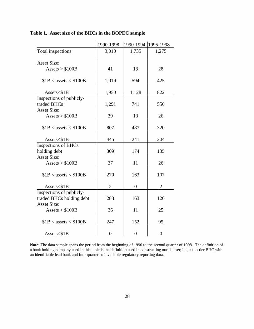
Table 1 summarizes our sample of inspections. The full sample contains 3,010 complete

inspections of 1,034 unique entities for which we know the assigned BOPEC rating, as well as

the rating leading into the inspection. Almost 65% of the BHCs in the sample are relatively

small, with less than $1 billion in total assets. Slightly more inspections occurred in the first half

of the sample than in the second half, reflecting consolidation in the U.S. banking sector.

There are 1,291 inspections of publicly traded BHCs, corresponding to 363 unique

entities. Note that publicly traded BHCs are generally larger than privately held BHCs, with a

greater percentage having total assets ranging between $1 billion and $100 billion. Of the 41

inspections of large BHCs (assets greater than $100 billion), 39 of the inspections are of publicly

traded BHCs.

10

With respect to BHCs with outstanding debt issues, this subsample contains 309 BOPEC

ratings corresponding to 63 unique BHCs. Again, these BHCs are typically larger than those in

the full sample with almost all BHCs having between $1 billion and $100 billion in assets.

Finally, there are 283 BOPEC ratings corresponding to 58 unique BHCs that have both

publicly traded equity and debt outstanding. As expected, these BHCs are also typically larger

with almost all having between $1 billion and $100 billion in assets.

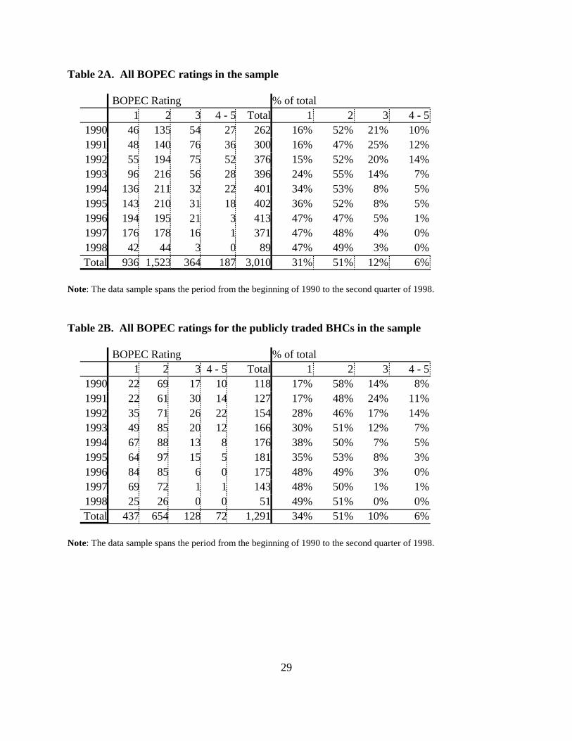
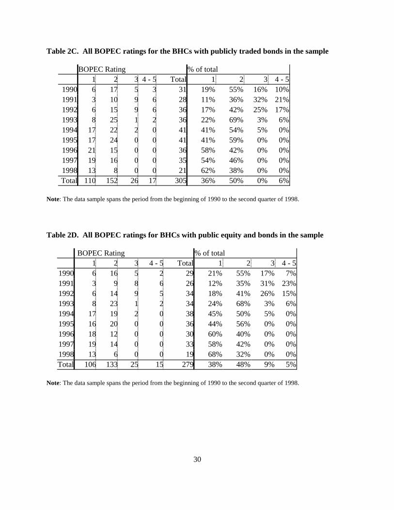
Tables 2A-2D present the distribution of BOPEC ratings assigned in each year for all

BHCs, for BHCs with publicly traded equity, for BHCs with publicly traded bonds, and BHCs

with both public equity and debt, respectively. The majority of the ratings fall in the upper two

categories, indicating that a BHC’s financial condition and risk profile are of little supervisory

concern. For the full sample, while the distribution of ratings fluctuates over time, the

percentage of ratings in the top two categories never falls below 63%. The maximum value is

96.5% in 1998. Note that there are very few inspections culminating in a BOPEC rating of 4 or

worse, since both supervisors and bankers actively try to prevent this outcome.

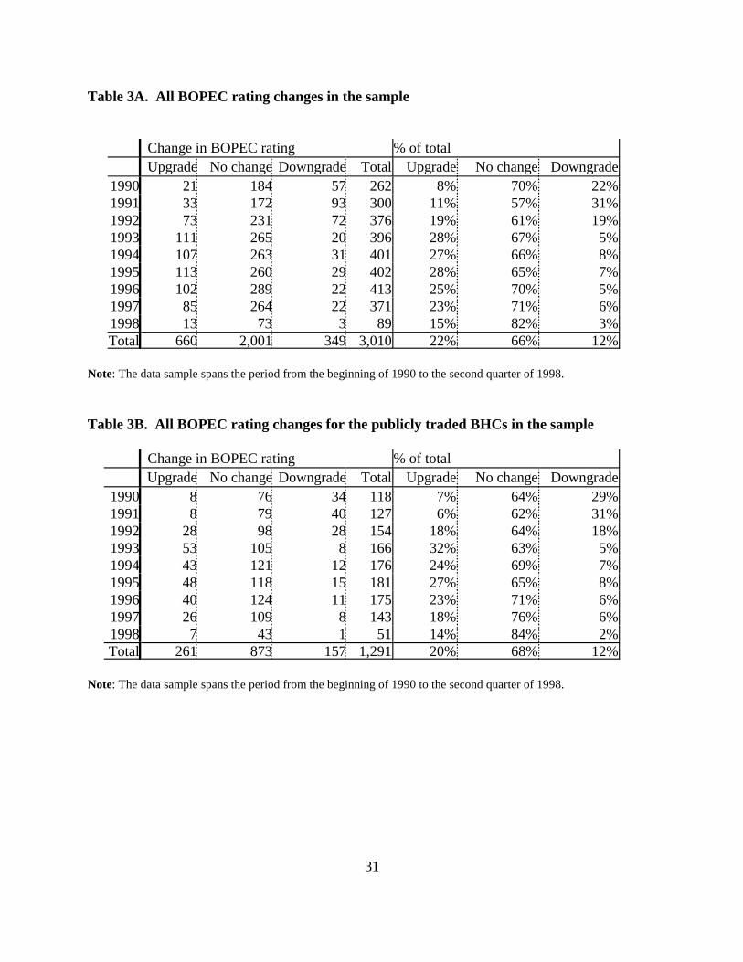
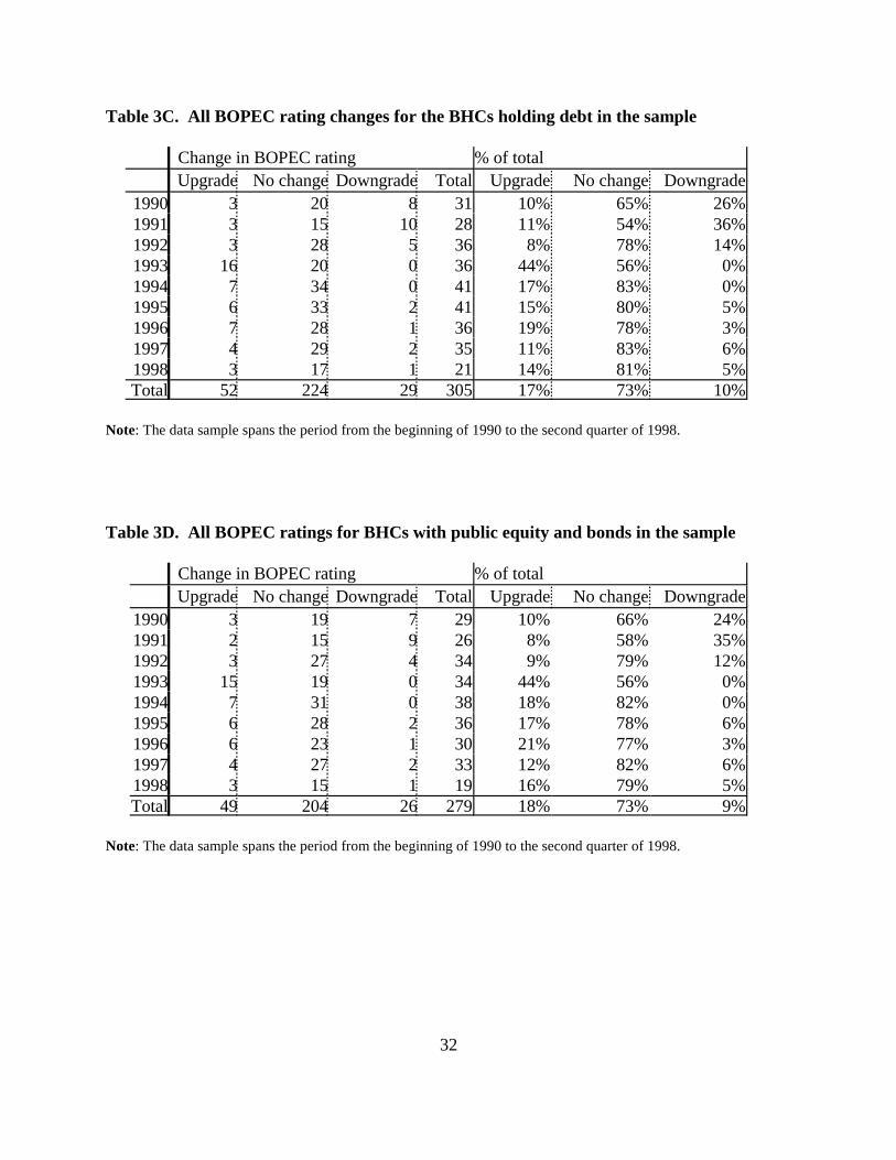
Tables 3A-3D present the pattern of changes in the BOPEC ratings in our sample. The

most frequent outcome is no change in BOPEC rating, accounting for between 69% and 87% of

the annual totals for the full sample and the equity subsample. The pattern of BOPEC upgrades

and downgrades fluctuates dramatically over the course of the sample time period. For all four

samples, from 1990 through 1992, more downgrades occurred than upgrades, but from 1993

through the end of the sample, the pattern was reversed. The pattern appears to follow the

general trends in U.S. banking and macroeconomic conditions during the 1990s.

III. Multivariate analysis using the ordered logit model

Our proposed BOPEC off-site monitoring (BOM) model is an ordered logit model, and is

similar in structure to the SEER model for CAMELS ratings. We assume that the BOPEC rating

assigned to BHC i in quarter t, denoted BP*it, can be modeled as

(1) ( )*it E Eit 1 D Dit 1 it 2 E Eit 1 D Dit 1 itBP I I x z z ,− − − − −= β + γ + γ + π + π + ε

14 See Gunther and Moore (2000).

11

In this specification, xit-2 is a (k×1) vector of supervisory variables unique to BHC i observed two

quarters prior to the BOPEC assignment. The indicator variables IEit-1 and IDit-1 represent BHCs

with publicly traded equity and debt, respectively, a quarter prior to the BOPEC assignment. We

choose to lag the supervisory variables by two quarters because these are often the most recent

data available to the holding company inspection team at the time of inspection.14 The

interaction terms allow us to control for possible differences between BHCs with and without

public equity and debt. The zEit-1 and zDit-1 terms are vectors of equity and debt market variables,

respectively, that correspond to BHC i at time t-1, one quarter before the BOPEC assignment.

The supervisory variables and the financial market variables enter into the model with different

lags since securities market information is available on a more timely basis than is supervisory

information. The error term �it has a standard logistic distribution.

III.A.1: Supervisory Variables

The choice of which supervisory variables to include in xit-2 is challenging. No simple

behavioral models exist of how supervisors assign BOPEC ratings and, as mentioned, there are

more than 800 variables at the supervisors' disposal for this purpose. For this study, we selected

nine explanatory variables that are reasonable proxies for the five components of the BOPEC

rating. As in Krainer and Lopez (2001), we chose a parsimonious specification in the hopes of

generating reasonable out-of-sample forecasts. Additionally, we face the practical concern that

many fewer BOPEC ratings are available in any given subsample period than are available in our

full sample.

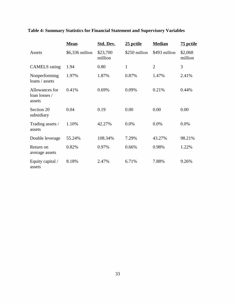
We use ten explanatory variables in this study; see Table 4 for summary statistics. The

first variable is the natural log of total BHC assets, which is our control variable for BHC size.

The next four variables are used to capture the supervisory concerns regarding the BHC's bank

subsidiaries, as summarized in the “B” component of the rating. The second variable is the

CAMELS rating of the BHC's lead bank. The third variable is the ratio of the BHC's

nonperforming loans, nonaccrual loans, and other real estate owned to its total assets. This

15 Note that the trading assets variable as currently reported first became available in the first quarter of1995. Before then, we proxy for BHC trading assets using the sum of the self-reported replacement cost of interestrate and foreign exchange derivative contracts.

16 A variety of capital measures have been used in previous studies, such as Evanoff and Wall (2000) andEstrella et al. (2000). We chose a simple measure to facilitate comparison over the entire ten-year period.

12

variable proxies for the health and performance of the BHC’s loan portfolio. The fourth variable

is the ratio of the BHC’s allowances (or provisions) for losses on loans and leases to its total

loans, another proxy for the health and performance of the BHC’s loan portfolio.

The fifth variable is an indicator of whether the BHC has a Section 20 subsidiary, which

is a subsidiary that can engage in securities activities that commercial banks were not permitted

to engage in before the Gramm-Leach-Bliley Act of 1999. This variable is a proxy for the scale

of the BHC’s nonbank activities, and thus speaks to the “O” component of the BOPEC rating.

We also include as the sixth variable the ratio of a BHC's trading assets to its total assets as a

proxy of its non-banking activities, whether conducted in banking or non-banking subsidiaries.15

The seventh variable is the so-called “double leverage” ratio between the BHC and its

lead bank, which is the ratio of the lead bank's equity capital to that of the parent's equity capital.

This variable provides a measure of the soundness of the parent BHC, indicating the extent to

which the parent's equity capital can be used to buffer against damage to the lead bank's equity

capital. We use this variable as a proxy for the condition of the parent BHC as summarized in the

“P” component of the BOPEC rating.

The eighth variable is the BHC’s return on average assets (ROAA), defined as the ratio of

the four-quarter average of the BHC’s net income to the four-quarter average of its assets. This

variable is used to proxy for the “E” component of the BOPEC rating.

The ninth variable is the BHC's ratio of equity capital to its total assets. This variable is

used to proxy for the “C” component of the BOPEC rating.16

Finally, we include the lagged BOPEC rating as a tenth supervisory variable. This

variable is meant to capture any persistence in ratings, or serve as a proxy for any omitted

variables that themselves have persistence.

We refer to the version of the BOM model based on just the supervisory variables as the

core model. The equity BOM model extends the core model to include the variables from the

13

equity markets. The debt BOM model extends the core model to include the bond market

variables. Finally, the extended BOM model estimates all of the parameters in the equation.

IIIA.2: Equity Market Variables

The equity market variables used in this study are based on observed stock returns over a

six-month period that ends one quarter prior to the beginning of the inspection. Our two

variables are motivated by a decomposition of a BHC’s cumulative stock return into systematic

and idiosyncratic portions,

(2)R (a b R b ffit

t 2

1

i im mt if t itt 2

1

= −

−

=−

−

=−

−

∑ ∑∑= + + +) .εt 2

1

The first term on the right-hand-side of equation (2) is a predicted cumulative return based on a

two-factor model. The factors are the market return and the change in the federal funds rate. The

factor loadings ai, bim, and bif are estimated over a 60 month sample period ending 12 months

prior to the BHC’s inspection. The difference between the actual cumulative return and the

predicted cumulative return is a residual, or a cumulative abnormal return. Dividing both sides

of the above equation by the standard error of the cumulative abnormal return yields a

representation of an “adjusted” cumulative return as a function of an adjusted systematic

cumulative return plus a standardized cumulative abnormal return (SCAR).

The motivation behind using stock market data lies in the hope that there is some

agreement between stock market investors and supervisors on what constitutes healthy financial

condition. Stock market investors are clearly not trying to forecast BOPEC ratings. But if the

same financial developments that lead to a supervisory ratings change also lead to changes in

expected stock returns, then it is possible that regulators can use stock market signals as

indicators of what they themselves might do if they were to inspect the BHC.

BHC stock price changes that are unusually large in magnitude with respect to general

market activity may signal changes in condition that will eventually lead to a ratings change. The

SCAR variable is designed specifically for identifying which stock price changes are “unusually

large.” However, relying exclusively on SCARs for market signals may cause us to miss

important information in stock prices. For example, an economy-wide shock that lowers returns

17 For a discussion of the market for BHC subordinated debt, see Kwast et.al. (1999), Hancock and Kwast(2000), Feldman and Schmidt (2000), and Goyal (1998).

14

for the entire banking sector might not translate into abnormally negative returns for any

particular BHC, but could very well be an early indicator for changes in supervisory ratings

sector-wide.

For a variety of reasons, these equity market variables are not available for all publicly

traded BHCs over the entire sample period. For example, we cannot generate reliable SCARs

when a BHC does not have at least five years of stock return data with which to estimate the

two-factor market model. To address this issue, we replaced these missing values with the

variable’s in-sample mean for the available observations, as per Griliches (1986). We also

include fixed effects to account for this data adjustment. This procedure does not affect the

model’s coefficient estimates for the variables with missing values, but allows us to use the entire

sample in our estimation.

III.A.3: Debt Market Variables

The debt market variables used in this study are changes in bond yields taken from the

Warga/Lehmann Brothers Corporate Bond Database. These are the same data used by Bliss and

Flannery (2001). The source of the data is the Warga / Lehman Brothers Corporate Bond

Database. Note that this database includes both subordinated and non-subordinated BHC debt.17

There are two empirical issues that are unique to bond data. First, in cases where a BHC has

multiple outstanding bonds, it is necessary to compress this market information into a single

observation. In this case, we use a weighted average change in bond yield for the debt market

variable, where the weights correspond to the size of the issue relative to the BHC’s total amount

of bonds outstanding in the quarter.

Second, as with the stock market variables, we would like to have some measure of what

constitutes an abnormal change in yield. Here, we follow Bliss and Flannery and compute debt

spreads from bond price indices based on term-to-maturity and rating buckets (either using

Moody’s or S&P ratings to produce two sets of indices). The Bliss and Flannery ratings buckets

consist of 11 categories that correspond to Moody’s and S&P ratings and three term-to-maturity

18 The ‘+’ or ‘-‘ qualifiers attached to the basic rating definitions are suppressed.. The maturity buckets areless than 5 years, 5-10 years, and greater than 10 years.

19 In our empirical work to date we used just two of the Bliss and Flannery bond indices. We examinedchange in average BHC bond yield relative to the index composed of similar rated/term bonds (i.e., all the bonds) asrated by Moody’s. We examined both the equally weighted and the amount-outstanding weighted indices. Theresults were similar, so we report just the results for the amount-outstanding weighted index.

15

categories.18 The Bliss and Flannery indices allow us to study changes in yields relative to an

index of similar bonds drawn from all industries.19 This adjustment allows us to concentrate on

changes in yields that are purged of larger, systematic factors.

We will also find it useful to subtract out yield spread changes from the bonds of BHCs

with similar supervisory ratings to arrive at a variable more closely related to the abnormal

returns used in the stock market data. For BHC i with BOPEC rating j at time t, we define a

yield spread of a bond with terms k as

(3) ,ijkt ijkt kts y y= −

where is the yield on an index of like-termed bonds. We define the adjusted yield spread askty

(4) ,ijkt ijkt jtd s s= −

where is the median yield spread from the set of all BHCs with BOPEC rating j at time t andjts

publicly traded debt. In our empirical work, these “abnormal” changes in bond yield spreads

appear to have more predictive power than the simple changes in yield relative to the all bonds

index. In the empirical analysis to follow, we use only the adjusted yield spreads defined in (4).

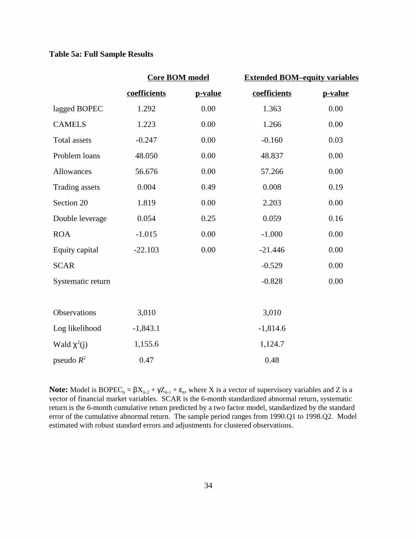
III.B. Empirical results

We estimate four versions of the BOM model; i.e.,

(5) ( )*it E Eit 1 D Dit 1 it 2 E Eit 1 D Dit 1 itBP I I x z z .− − − − −= β + γ + γ + π + π + ε

For the core model, we set �E = �D = 0. For the equity BOM model, we set �D =0. For the debt

BOM model, we set �D = 0. For the extended BOM model, we do not constrain any of the

parameters. The empirical results for the full sample of BOPEC observations are presented in

16

Tables 5A and 5B. Note that while we estimate the model with complete sets of interactions for

the supervisory variables, we do not report the coefficients on the interacted variables for

purposes of economizing on space.

In the full sample, the coefficients on the financial market variables are statistically

significant at conventional levels. The equity market variables have negative signs, which is to

be expected; positive values for both abnormal and predicted returns tend to be associated with

lower (better) BOPEC ratings. For the debt market variable, the positive sign is also in line with

expectations. Higher yield spreads relative to a ratings-specific composite are associated with

higher (worse) BOPEC ratings.

The likelihood ratio results indicate that incorporating securities market information

improves the core BOM model’s in-sample fit. The likelihood ratio test statistic for the equity

market BOM model relative to the core BOM model is 57.0, which has a p-value of 0.0% under

the �2(3) distribution. The likelihood ratio test statistic for the debt market BOM model relative

to the core BOM model is 6.6, which has a p-value of 10.0% for the �2(2) distribution. Finally,

the likelihood ratio test statistic for the equity-debt BOM model relative to the simple BOM

model is 106.6, which has a p-value of 0.0% under the �2(5) distribution.

Clearly, the results indicate that using some type of securities market information in the

BOM model is appropriate. However, again using likelihood ratio statistics, we find that using

both sources is better than using either one alone. The likelihood ratio test statistic for the

equity-debt BOM model relative to the equity BOM model is 49.6, which has a p-value of 0.0%

for the �2(2) distribution. The likelihood ratio test statistic for the equity-debt BOM model

relative to the debt BOM model is 113.2, which has a p-value of 0.0% for the �2(3) distribution.

Hence, both sources of market information are shown to be useful complements to the chosen

supervisory information set.

III.C. The relative importance of debt and equity information

As mentioned in the introduction, one of the primary motivations for using both equity

and debt market data in a monitoring model is that no single information source is likely to

20 Gropp, Vesala and Vulpes (2001) use a similar measure.

17

dominate the other in all states of the world. For example, the residual claim feature of equity

suggests that equity market investors would be good at predicting upgrades, or predicting

changes in supervisory ratings when asset values are relatively far from the default point. Debt

market investors, by contrast might be more likely to predict downgrades, or predict changes in

supervisory ratings when asset values are relatively close to the default point.

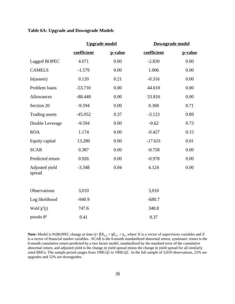
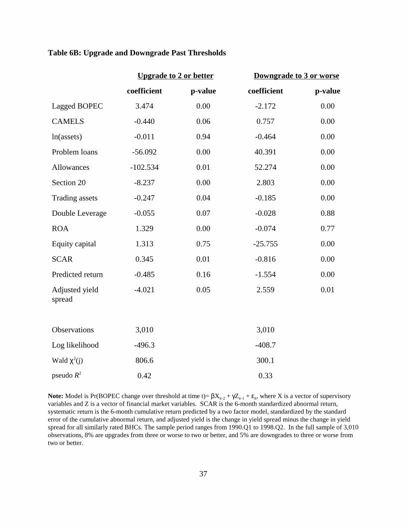
In this section, we study whether debt market and equity market variables have

differential ability to predict certain types of inspection outcomes. In Tables 6A and 6B, we

present the results from the estimation of upgrade and downgrade models. Unlike the analysis in

the previous section, the models used here are ordinary logit models where the dependent

variables are indicator variables of whether an upgrade or downgrade takes place or not at the

inspection. Interestingly, both sets of financial market variables have strong statistical

significance in both the upgrade and the downgrade models. This same basic result carries over

when we analyze transitions between the of-concern list (BOPEC 3-5) and the not-of-concern list

(BOPEC 1-2). Debt market signals appear to anticipate both upgrades and downgrades over

regulatory thresholds. Interestingly for the case of equity market variables, only the SCAR

consistently anticipates threshold transitions. For the case of upgrades to BOPEC 2 or better, the

systematic return variable is not statistically significant.

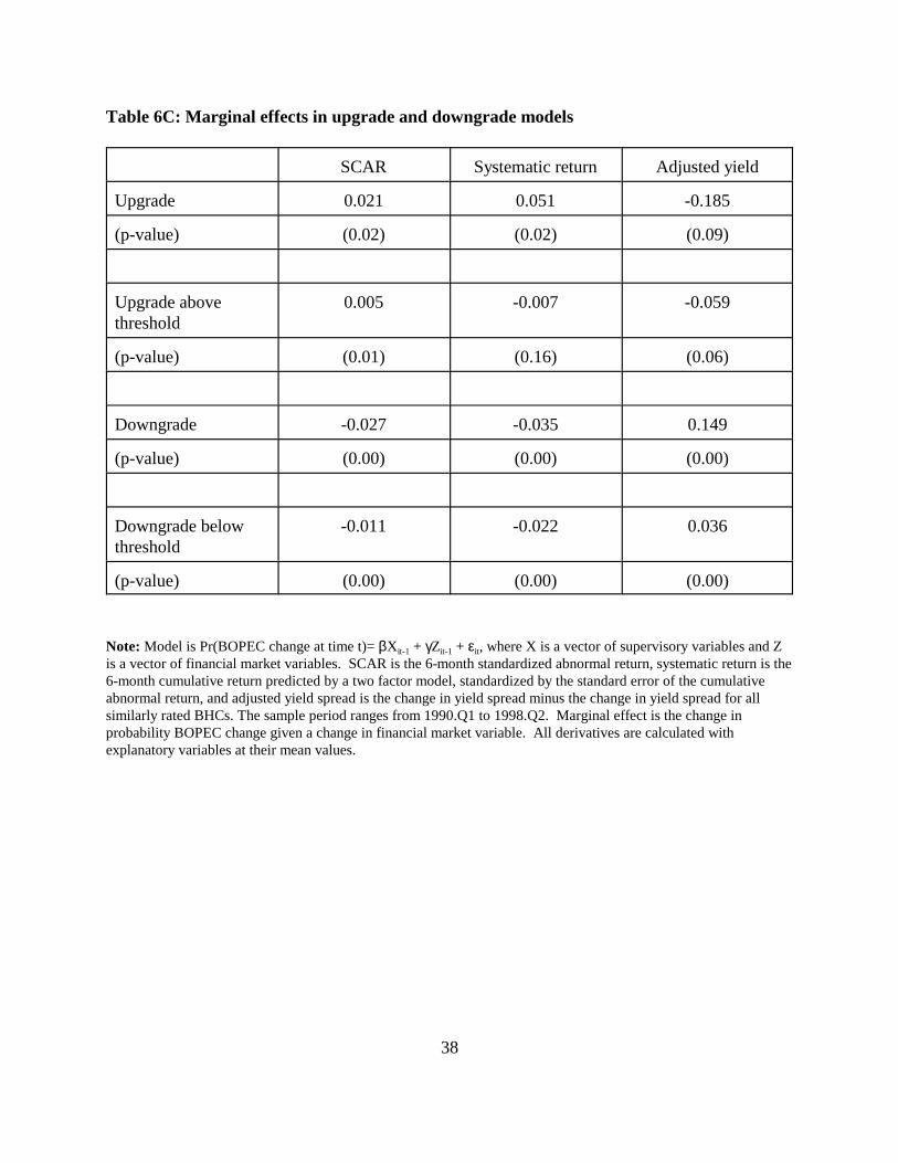
Debt and equity securities have payoffs that are nonlinear functions of the underlying

value of a firm’s assets. To investigate more closely whether these nonlinearities are important

for the relative significance of debt market and equity market signals, we conduct a simple

exercise of estimating a version of the BOM model that allows for the financial market variables

to have differential effects on supervisory ratings, depending on the market value of the BHC’s

assets. For this exercise we use a model of a firm’s asset value that is widely used in the

literature.20 As in Ronn and Verma (1986), we model asset value as a geometric Brownian

motion. The firm’s equity can be modeled as a call option,

18

(6)( ) ( ) ( ) ( )2 2

A AA

A A

ln A / D s / 2 ln A / D s / 2E AN DN s

s s,

+ += − −

where E is the market value of equity, A is the market value of assets, D is the book value of

debt, sA is the volatility (standard deviation) of changes in asset value, and N(x) is the standard

normal cumulative density function. Neither the market value of assets nor the volatility are

directly observable in the data. A second equation linking asset volatility to equity volatility

completes the model,

(7) A E2A

A

Es s .

ln(A / D) (s / 2)AN

s

=+

Essentially, the asset volatility is a de-levered equity volatility. Our distance-to-default is simply

the market value of assets minus the book value of liabilities (both in logs), all scaled by the

estimated asset volatility.

Working within the BOM framework, we create indicator variables that take the value

one if a BHC’s distance-to-default is in a certain percentile of the overall distribution of distance-

to-default, and zero otherwise. We then interact this indicator variable with the market signals.

Since this exercise requires us to restrict the sample to include just BHCs with publicly traded

securities, we include the lagged BOPEC rating as the lone supervisory variable in the model.

Formally, the model is,

(8) , 2 , , 1 , 1 ,( )it i t n i t i t i tBP BP I zβ π α ε− − −= + + +

where Z is the financial market variable in question and Init-1 is equal to one if BHC i’s distance-

to-default is in the nth percentile at time t-1, and zero otherwise.

The results from this exercise are in Tables 7A and 7B. In Table 7A, the regressions are

based on 1,266 inspections for BHCs with publicly traded equity. For this exercise, we restrict

our attention purely to the SCAR. In Table 7B, the regressions are based on 282 inspections of

firms with publicly traded equity and debt. In 7B, we restrict our attention purely to the adjusted

19

bond spread.

Our main object of interest is whether the coefficients on the financial market variables

are different in magnitude depending on how close the BHC is to its default point. For example,

for the case of debt market information, we expect the coefficients to be positive–large abnormal

changes in yield spreads should signal increases in the BOPEC rating, or downgrades. But we

would also expect the coefficient to be larger in magnitude if the BHC is closer to default (that is,

α > 0). For the case of the stock market variable, we expect the coefficients on the SCAR to be

negative, but the total effect of the SCAR on the BOPEC rating should be muted for BHCs close

to default (again, α > 0).

In Table 7A we see that when we allow for a differing impact of the SCAR variable on

assigned BOPEC ratings, our basic predictions are borne out. The coefficient on the SCAR is

invariably negative and statistically significant, and α is estimated to be positive (although, the

latter estimate is not significantly different from zero) for most close-to-default cutpoints. Thus,

the stock market appears to send a stronger signal when BHCs are defined to be far from default.

This is true for most definitions of what it means to be close to default. Note that the choice of

which percentile to use in the definition of the indicator variable Init-1 has no impact on the overall

fit of the model. The pseudo-R2 in each model is 0.31.

In Table 7B we see further evidence of the impact of distance-to-default on the coefficient

estimate on the bond market variable. The coefficient estimate for α is always positive, and

sometimes is large in magnitude. For BHCs in the bottom 10th percentile of the distance-to-

default distribution, the estimated magnitude of the signal from the bond markets is more than

three times as large as when a BHC is further from default. As the definition of close to default

becomes more inclusive, however, the close-to-default coefficient ceases to be significant. When

close to default is defined as belonging to the bottom 80th percentile (implying that virtually all

BHCs are in this category), then the close-to-default coefficient is significant again, but at the

expense of statistical significance for the adjusted yield spread variable. As in the exercise with

the SCAR variable in Table 7A, the choice of which percentile to use in the definition of the

indicator variable Init-1 has no impact on the overall fit of the model. The pseudo-R2 in each

model is 0.41.

20

In summary, we detect an asymmetric contribution of debt and equity market signals to

explaining BOPEC ratings that depends on how close the BHC is to its default point. The

coefficients on the equity market signals are largest in magnitude for the case of BHCs defined to

be far from default. Coefficients on the adjusted yield spreads are much larger in magnitude for

BHCs defined to be very close to default.

III.D. Out-of-sample performance

For supervisors, the true test of usefulness of an empirical model is whether the model

has any predictive power out of sample. As in Krainer and Lopez (2001), we evaluate the

model’s forecasting ability by estimating a series of rolling logits and compare the model’s

predicted BOPEC ratings to the realized BOPECs. Specifically, we estimate various

specifications of the model using four quarters of data and then use the estimated coefficients to

predict BOPEC ratings awarded in the next quarter. Clearly, the subsamples available for

estimation in any given period will be small relative to the full sample. However, we accept this

small sample size because this type of exercise would, presumably, simulate the way market data

would be used if supervisors were to adopt it formally.

Our measure of whether the model forecasts well or not is to ask how often model

predictions are borne out. For example, if the model generates a signal suggesting an upgrade,

what percentage of the time will an upgrade actually take place? The upgrade (downgrade)

predictions in the tables are based on forecasted ratings that are a full rating better (worse) than

the current rating. For the core model, an upgrade signal received four quarter prior to inspection

materializes into an actual upgrade 52% of the time (Table 8A). Consequently, an upgrade signal

at four quarters prior is incorrect 48% of the time–35% of the time the actual outcome of the

inspection is no change in rating, and 13% of the time the actual outcome is a downgrade. By

one quarter prior to the inspection, the upgrade signal is accurate 90% of the time. The model

appears to be just as effective at picking up downgrades. Four quarters prior to the inspection, a

downgrade signal is accurate 69% of the time, improving to 90% accuracy one quarter prior to

the inspection.

These results are quite promising. In the full sample, the unconditional probabilities of

21

upgrades, downgrades, and no change at the inspection are 22%, 12%, and 66%, respectively.

Thus, the conditioning information in the model is clearly useful relative to the unconditional

probabilities. This notion is formalized by the Pearson tests (contained in the right-most

column), which test whether the conditional probabilities generated by the model are statistically

different from the unconditional probabilities.

Model accuracy is little changed after incorporating financial market data. In Table 8B

we see that when the debt market variable is added, the model’s forecasting accuracy is actually a

little worse than the accuracy of the simple model with only supervisory variables. An upgrade

signal four quarters prior to the inspection is correct 46% of the time, compared to 52% of the

time for the core model. A downgrade signal four quarters prior to the eventual inspection

results in an actual downgrade 63% of the time, compared with 69% for the core model.

With the equity market data (Table 8C), the results are somewhat better for the case of

upgrades. Signal accuracy increases from 62% four quarters prior to inspection to 91% accuracy

within one quarter of the inspection. This compares to 52% and 90%, respectively, for the core

model. For downgrades, forecast accuracy improves from 56% to 82% as the inspection

approaches, not quite as good an improvement in accuracy as observed in the core model.

Forecasting accuracy of the extended model with both equity and debt market variables is nearly

indistinguishable from the accuracy of the core model (Table 8D).

In summary, the forecasting accuracy of the extended models looks very similar. This is

formalized by the Pearson statistics reported in the rightmost columns of Tables 8B-8C, where

we test whether the probabilities of BOPEC rating changes generated by the extended models are

statistically different from the conditional probabilities generated by the core model. By and

large, the extended models fail to generate forecasts that are different from the core model

forecasts at conventional levels of significance.

III.E. Information in the Forecasts

The forecasts of BOPEC ratings at upcoming inspections do not appear to be appreciably

different across the core and the extended models. This result, however, does not mean that the

individual BOPEC rating changes correctly forecasted by the two models are the same. The

21 It must be acknowledged these differences in the set of correct forecasts of ratings changes could beevidence of parameter instability in our model.

22

forecasting literature has shown that combining forecasts from different models can improve

certain aspects of forecast accuracy. That appears to be the case here, since the two models

signal BOPEC changes for different, although overlapping, sets of BHCs. Hence, another way to

gauge the contribution of equity market information is to examine the additional forecast signals

for public BHCs as generated by the extended model relative to the core model’s signals. Seen in

this light, the marginal benefit of adding these additional signals to the signals from the core

model is notable.21

In Table 9A we focus exclusively on downgrades. We define a downgrade signal as a

forecasted BOPEC rating that is greater than the current rating by one or more. Using signals

generated by both the core and the extended models, we ask what is the percentage increase in

correct signals when financial market data are used in the BOM model? For the complete model

with bond yields and stock return data, the extended model produces 9% more correct signals at

the four quarter horizon over and above those produced by the core model. By the 1 quarter

horizon, the model produces 37% more signals. All the extended models show an increasing rate

of marginal usefulness as the inspection grows near. All of these additional correct forecasts are

for ratings changes at BHCs with publicly traded securities.

One other interesting point in Table 9A is the similarity between the marginal

contributions of the debt and equity model and the equity market alone model. Evidently, in this

particular forecasting framework, most of the additional signals a supervisor can extract from

financial market data come from the equity markets. This result contrasts with the in-sample

results and may be due to the relatively small number of BHCs with publicly traded debt in any

given subsample period.

Of course, the extended model produces incorrect signals over and above those produced

by the core model. Given that Table 9A shows that the extended model helps to identify

additional BOPEC ratings changes, these mistakes may be responsible for our earlier result that

the forecast accuracy of the core and extended models is virtually the same. We look at this

tradeoff more closely in table 9B, where we express the ratio of correct signals to incorrect

23

signals. For example, in the case of the debt and equity model at the four quarter horizon, the

model produces 1 extra correct signal at the cost of 4 incorrect downgrade signals. By the 1

quarter horizon, however, the accuracy dramatically improves. The extended model produces 4

extra correct signals at the cost of only one extra incorrect signal. The model extended by debt

and equity and the model extended by equity market data alone behave quite similarly.

Interestingly, the correct signal / incorrect signal tradeoff for the model extended with debt

market information is quite good. By one quarter out, the extended model produces 6 correct

signals for every incorrect signal. However, the drawback to this model is that it produces

relatively fewer signals over and above the core model.

IV. Conclusion

In conclusion, our empirical results indicate that both equity and debt market information

are useful in improving the in-sample fit of our proposed BOM model for BOPEC ratings. Both

types of financial market information appear to be useful in explaining both upgrades and

downgrades. Moreover, we are able to detect nonlinearities in the impact of financial market

variables on BOPEC ratings. Close to default, the estimated effect of changes in yield spreads on

BOPEC ratings is larger in magnitude for than it is for BHCs far from default, and vice-versa for

equity market data.

When we turn to out-of-sample forecasting, however, evidence for the usefulness of

market information is disappointingly weak. We adopt a methodology of estimating the BOM

model’s coefficients on a rolling subsample of data and then forecasting BOPEC ratings into the

future. We find the forecast accuracy of the models extended by financial market data is not

much different than the accuracy of the core model based on supervisory data alone.

Finally, while the out-of-sample forecasting accuracy of the core and extended models is

similar, we note that the actual forecasts are quite different. That is, the core model correctly

identifies one set of BOPEC ratings changes, while the extended model correctly identifies

another set of ratings changes. We show that the extended model correctly identifies additional

ratings changes for publicly traded BHCs over and above the correct forecasts in the core model.

These additional correct forecasts can be achieved at a relatively modest cost of additional

24

incorrect signals.

25

References

Basel Committee on Banking Supervision, 2001. "The New Basel Accord." Consultative Paper,Bank for International Settlements. (http://www.bis.org/publ/bcbsca.htm)

Berger, A. N., and Davies, S. M., 1998. "The Information Content of Bank Examinations,"Journal of Financial Services Research, 14, 117-144.

Berger, A.N., Davies, S.M., and Flannery, M.J., 2000. "Comparing Market and SupervisoryAssessments of Bank Performance: Who Knows What When?," Journal of Money,Credit and Banking, 32, 641-667.

Bliss, R., 2000. "The Pitfalls in Inferring Risk from Financial Market Data," Manuscript,Economic Research Department, Federal Reserve Bank of Chicago.

Bliss, R. and Flannery, M., 2001. "Market Discipline in the Governance of U.S. Bank HoldingCompanies: Monitoring versus Influence," in R. Mishkin, ed. Prudential Supervision:Why Is It Important and What are the Issues?. NBER. Forthcoming.

Board of Governors of the Federal Reserve System, 1995. Supervisory Letter 95-43: RevisedBank Holding Company Surveillance Procedures. http://www.federalreserve.gov/boarddocs/SRLETTERS/1995/sr9543.htm.

Board of Governors of the Federal Reserve System, 2002. Supervisory Letter 02-01: Revisionsto Bank Holding Company Supervision Procedures for Organizations with TotalConsolidated Assets of $5 Billion or Less.http://www.federalreserve.gov/boarddocs/SRLETTERS/2002/sr0201.htm

Campbell, J., Lo, A., and MacKinlay, A., 1997. The Econometrics of Financial Markets.Princeton University Press.

Cole, R.A., Cornyn, B.G. and Gunther, J.W., 1995. "FIMS: A New Monitoring System forBanking Institutions," Federal Reserve Bulletin, January, 1-15.

Cole, R.A. and Gunther, J.W., 1998. "Predicting Bank Failures: A Comparison of On- andOff-Site Monitoring Systems;" Journal of Financial Services Research, 13, 103-17.

Curry, T.J., Elmer, P.J. and Fissel, G., 2001. "Regulator Use of Market-Related Data to Improvethe Identification of Bank Financial Health," Manuscript, Federal Deposit InsuranceCorporation.

DeFerrari, L, and Palmer, D., 2001. "Supervision of Large Complex Banking Organizations."Federal Reserve Bulletin, February, 47-57.

26

DeYoung, R., Flannery, M., Lang, M., and Sorescu, S., 2001. "The Information Content BankExam Ratings and Subordinated Debt Prices." Journal of Money, Credit, and Banking,forthcoming.

Elmer, P.J. and Fissel, G., 2001. "Forecasting Bank Failure from Momentum Patterns in StockReturns," Manuscript, Federal Deposit Insurance Corporation.

Estrella, A., Park, S. and Peristiani, S., 2000. "Capital Ratios as Predictors of Bank Failure",Federal Reserve Bank of New York Economic Policy Review, July, 33-52.

Evanoff, D., and Wall, L., 2000. "Sub-debt Yield Spreads as Bank Risk Measures." Workingpaper #2000-24, Federal Reserve Bank of Atlanta.

Feldman, R. and Schmidt, J., 2000. “Granger Tests of Subordinated Debt Spreads and KMVExpected Default Frequencies,” Manuscript, Banking Supervision and RegulationDepartment, Federal Reserve Bank of Minneapolis.

Flannery, M., 1998. "Using Market Information in Prudential Bank Supervision," Journal ofMoney, Credit, and Banking, August, Part I, 273-305.

Flannery, M.J., 2001. “The Faces of ‘Market Discipline’,” Manuscript, University of Florida.

Flannery, M., Kwan, S., and Nimalendran, M., 2000. "Market Evidence on the Opaqueness ofBanking Firms' Assets," Manuscript, Federal Reserve Bank of San Francisco.

Flannery, M., and Sorescu, S., 1996. "Evidence of Bank Market Discipline in SubordinatedDebenture Yields: 1983-1991." Journal of Finance, 51, 1347-1377.

Gilbert, A., Meyer, A. and Vaughn, M., 2001. “Can Feedback from the Jumbo CD MarketImprove Off-Site Surveillance of Small Banks?,” Manuscript, Economic ResearchDepartment, Federal Reserve Bank of St. Louis.

Goyal, V.K., 1998. “Market Discipline of Bank Risk: Evidence from Subordinated DebtContracts,” Manuscript, Department of Finance, Hong Kong University of Science andTechnology.

Griliches, Z., 1986. "Economic Data Issues," in Griliches, Z. and Intriligator, M.D., eds.Handbook of Econometrics, Volume III. Elsevier Science Publishers BV.

Gropp, R., Vesala, J. and Vulpes, G., 2002. “Equity and Bond Market Signals as LeadingIndicators of Bank Fragility,” Manuscript, European Central Bank.

Gunther, J.W., Levonian, M.E. and Moore, R.R., 2001. "Can the Stock Market Tell Bank

27

Supervisors Anything They Don’t Already Know?," Federal Reserve Bank of DallasEconomic and Financial Review, Second Quarter, 2-9.

Gunther, J.W. and Moore, R.R., 2000. "Early Warning Models in Real Time," Financial IndustryStudies Working Paper #1-00, Federal Reserve Bank of Dallas.

Hall, J.R., King, T.B., Meyer, A.P. and Vaughn, M.D., 2001. "What Can Bank Supervisors Learnfrom the Equity Markets? A Comparison of the Factors Affecting Market-Based RiskMeasures and BOPEC Scores," Manuscript, Federal Reserve Bank of St. Louis.

Hancock, D., and Kwast, M., 2000. "Using Subordinated Debt to Monitor Bank HoldingCompanies: Is it Feasible?" Manuscript, Board of Governors of the Federal ReserveSystem.

Hirtle, B. and Lopez, J.A., 1999. “Supervisory Information and the Frequency of BankExaminations,” Federal Reserve Bank of New York Economic Policy Review, April, 1-20.

Krainer, J. and Lopez, J.A., 2001. “Incorporating Equity Market Information into SupervisoryMonitoring Models,” Federal Reserve Bank of San Francisco Working Paper #2001-14.

Kwast, M., et. al., 1999. "Using Subordinated Debt as an Instrument of Market Discipline:Report of the Study Group on Subordinated Notes and Debentures." Federal ReserveSystem Staff Study # 172, Board of Governors of the Federal Reserve System.

Merton, R., 1974. "On the Pricing of Corporate Debt: The Risk Structure of Interest Rates."Journal of Finance. 29, 449-470.

Meyer, P. and Pifer, H., 1970. “Prediction of Bank Failures,” Journal of Finance, 25, 853-868.

Pettway, R.H. and Sinkey, J.F., 1980. “Establishing On-Site Bank Examination Priorities: AnEarly-Warning System using Accounting and Market Information,” Journal of Finance,35, 137-150.

Sinkey, J.E., 1975. “A Multivariate Statistical Analysis of the Characteristics of Problem Banks,”Journal of Finance, 20, 21-36.

Sahajwala, R. and Van der Bergh, P., 2000. “Supervisory Risk Assessment and Early WarningSystems,” Basel Committee on Banking Supervision Working Paper No. 4, Bank forInternational Settlements.

28

Table 1. Asset size of the BHCs in the BOPEC sample

1990-1998 1990-1994 1995-1998Total inspections 3,010 1,735 1,275

Asset Size: Assets > $100B 41 13 28

$1B < assets < $100B 1,019 594 425

Assets<$1B 1,950 1,128 822Inspections of publicly-traded BHCs 1,291 741 550Asset Size: Assets > $100B 39 13 26

$1B < assets < $100B 807 487 320

Assets<$1B 445 241 204Inspections of BHCsholding debt 309 174 135Asset Size: Assets > $100B 37 11 26

$1B < assets < $100B 270 163 107

Assets<$1B 2 0 2Inspections of publicly-traded BHCs holding debt 283 163 120Asset Size: Assets > $100B 36 11 25

$1B < assets < $100B 247 152 95

Assets<$1B 0 0 0

Note: The data sample spans the period from the beginning of 1990 to the second quarter of 1998. The definition ofa bank holding company used in this table is the definition used in constructing our dataset; i.e., a top-tier BHC withan identifiable lead bank and four quarters of available regulatory reporting data.

29

Table 2A. All BOPEC ratings in the sample

BOPEC Rating % of total 1 2 3 4 - 5 Total 1 2 3 4 - 5

1990 46 135 54 27 262 16% 52% 21% 10%1991 48 140 76 36 300 16% 47% 25% 12%1992 55 194 75 52 376 15% 52% 20% 14%1993 96 216 56 28 396 24% 55% 14% 7%1994 136 211 32 22 401 34% 53% 8% 5%1995 143 210 31 18 402 36% 52% 8% 5%1996 194 195 21 3 413 47% 47% 5% 1%1997 176 178 16 1 371 47% 48% 4% 0%1998 42 44 3 0 89 47% 49% 3% 0%Total 936 1,523 364 187 3,010 31% 51% 12% 6%

Note: The data sample spans the period from the beginning of 1990 to the second quarter of 1998.

Table 2B. All BOPEC ratings for the publicly traded BHCs in the sample

BOPEC Rating % of total1 2 3 4 - 5 Total 1 2 3 4 - 5

1990 22 69 17 10 118 17% 58% 14% 8%1991 22 61 30 14 127 17% 48% 24% 11%1992 35 71 26 22 154 28% 46% 17% 14%1993 49 85 20 12 166 30% 51% 12% 7%1994 67 88 13 8 176 38% 50% 7% 5%1995 64 97 15 5 181 35% 53% 8% 3%1996 84 85 6 0 175 48% 49% 3% 0%1997 69 72 1 1 143 48% 50% 1% 1%1998 25 26 0 0 51 49% 51% 0% 0%Total 437 654 128 72 1,291 34% 51% 10% 6%

Note: The data sample spans the period from the beginning of 1990 to the second quarter of 1998.

30

Table 2C. All BOPEC ratings for the BHCs with publicly traded bonds in the sample

BOPEC Rating % of total1 2 3 4 - 5 Total 1 2 3 4 - 5

1990 6 17 5 3 31 19% 55% 16% 10%1991 3 10 9 6 28 11% 36% 32% 21%1992 6 15 9 6 36 17% 42% 25% 17%1993 8 25 1 2 36 22% 69% 3% 6%1994 17 22 2 0 41 41% 54% 5% 0%1995 17 24 0 0 41 41% 59% 0% 0%1996 21 15 0 0 36 58% 42% 0% 0%1997 19 16 0 0 35 54% 46% 0% 0%1998 13 8 0 0 21 62% 38% 0% 0%Total 110 152 26 17 305 36% 50% 0% 6%

Note: The data sample spans the period from the beginning of 1990 to the second quarter of 1998.

Table 2D. All BOPEC ratings for BHCs with public equity and bonds in the sample

BOPEC Rating % of total1 2 3 4 - 5 Total 1 2 3 4 - 5

1990 6 16 5 2 29 21% 55% 17% 7%1991 3 9 8 6 26 12% 35% 31% 23%1992 6 14 9 5 34 18% 41% 26% 15%1993 8 23 1 2 34 24% 68% 3% 6%1994 17 19 2 0 38 45% 50% 5% 0%1995 16 20 0 0 36 44% 56% 0% 0%1996 18 12 0 0 30 60% 40% 0% 0%1997 19 14 0 0 33 58% 42% 0% 0%1998 13 6 0 0 19 68% 32% 0% 0%Total 106 133 25 15 279 38% 48% 9% 5%

Note: The data sample spans the period from the beginning of 1990 to the second quarter of 1998.

31

Table 3A. All BOPEC rating changes in the sample

Change in BOPEC rating % of total Upgrade No change Downgrade Total Upgrade No change Downgrade

1990 21 184 57 262 8% 70% 22%1991 33 172 93 300 11% 57% 31%1992 73 231 72 376 19% 61% 19%1993 111 265 20 396 28% 67% 5%1994 107 263 31 401 27% 66% 8%1995 113 260 29 402 28% 65% 7%1996 102 289 22 413 25% 70% 5%1997 85 264 22 371 23% 71% 6%1998 13 73 3 89 15% 82% 3%Total 660 2,001 349 3,010 22% 66% 12%

Note: The data sample spans the period from the beginning of 1990 to the second quarter of 1998.

Table 3B. All BOPEC rating changes for the publicly traded BHCs in the sample

Change in BOPEC rating % of total Upgrade No change Downgrade Total Upgrade No change Downgrade

1990 8 76 34 118 7% 64% 29%1991 8 79 40 127 6% 62% 31%1992 28 98 28 154 18% 64% 18%1993 53 105 8 166 32% 63% 5%1994 43 121 12 176 24% 69% 7%1995 48 118 15 181 27% 65% 8%1996 40 124 11 175 23% 71% 6%1997 26 109 8 143 18% 76% 6%1998 7 43 1 51 14% 84% 2%Total 261 873 157 1,291 20% 68% 12%

Note: The data sample spans the period from the beginning of 1990 to the second quarter of 1998.

32

Table 3C. All BOPEC rating changes for the BHCs holding debt in the sample

Change in BOPEC rating % of total Upgrade No change Downgrade Total Upgrade No change Downgrade

1990 3 20 8 31 10% 65% 26%1991 3 15 10 28 11% 54% 36%1992 3 28 5 36 8% 78% 14%1993 16 20 0 36 44% 56% 0%1994 7 34 0 41 17% 83% 0%1995 6 33 2 41 15% 80% 5%1996 7 28 1 36 19% 78% 3%1997 4 29 2 35 11% 83% 6%1998 3 17 1 21 14% 81% 5%Total 52 224 29 305 17% 73% 10%

Note: The data sample spans the period from the beginning of 1990 to the second quarter of 1998.

Table 3D. All BOPEC ratings for BHCs with public equity and bonds in the sample

Change in BOPEC rating % of total Upgrade No change Downgrade Total Upgrade No change Downgrade

1990 3 19 7 29 10% 66% 24%1991 2 15 9 26 8% 58% 35%1992 3 27 4 34 9% 79% 12%1993 15 19 0 34 44% 56% 0%1994 7 31 0 38 18% 82% 0%1995 6 28 2 36 17% 78% 6%1996 6 23 1 30 21% 77% 3%1997 4 27 2 33 12% 82% 6%1998 3 15 1 19 16% 79% 5%Total 49 204 26 279 18% 73% 9%

Note: The data sample spans the period from the beginning of 1990 to the second quarter of 1998.

33

Table 4: Summary Statistics for Financial Statement and Supervisory Variables

Mean Std. Dev. 25 pctile Median 75 pctile

Assets $6,336 million $23,700million

$250 million $493 million $2,068million

CAMELS rating 1.94 0.80 1 2 3

Nonperformingloans / assets

1.97% 1.87% 0.87% 1.47% 2.41%

Allowances forloan losses /assets

0.41% 0.69% 0.09% 0.21% 0.44%

Section 20subsidiary

0.04 0.19 0.00 0.00 0.00

Trading assets /assets

1.10% 42.27% 0.0% 0.0% 0.0%

Double leverage 55.24% 108.34% 7.29% 43.27% 98.21%

Return onaverage assets

0.82% 0.97% 0.66% 0.98% 1.22%

Equity capital /assets

8.18% 2.47% 6.71% 7.88% 9.26%

34

Table 5a: Full Sample Results

Core BOM model Extended BOM–equity variables

coefficients p-value coefficients p-value

lagged BOPEC 1.292 0.00 1.363 0.00

CAMELS 1.223 0.00 1.266 0.00

Total assets -0.247 0.00 -0.160 0.03

Problem loans 48.050 0.00 48.837 0.00

Allowances 56.676 0.00 57.266 0.00

Trading assets 0.004 0.49 0.008 0.19

Section 20 1.819 0.00 2.203 0.00

Double leverage 0.054 0.25 0.059 0.16

ROA -1.015 0.00 -1.000 0.00

Equity capital -22.103 0.00 -21.446 0.00

SCAR -0.529 0.00

Systematic return -0.828 0.00

Observations 3,010 3,010

Log likelihood -1,843.1 -1,814.6

Wald χ2(j) 1,155.6 1,124.7

pseudo R2 0.47 0.48

Note: Model is BOPECit = βXit-2 + γZit-1 + εit, where X is a vector of supervisory variables and Z is avector of financial market variables. SCAR is the 6-month standardized abnormal return, systematicreturn is the 6-month cumulative return predicted by a two factor model, standardized by the standarderror of the cumulative abnormal return. The sample period ranges from 1990.Q1 to 1998.Q2. Modelestimated with robust standard errors and adjustments for clustered observations.

35

Table 5b: Full Sample Results

Extended BOM–debt variables Extended BOM–equity and debtvariables

coefficients p-value coefficients p-value

lagged BOPEC 1.340 0.00 1.368 0.00

CAMELS 1.105 0.00 1.294 0.00

Total assets -0.133 0.01 -0.177 0.02

Problem loans 46.220 0.00 49.882 0.00

Allowances 70.835 0.00 59.132 0.00

Trading assets -0.002 0.77 0.008 0.20

Section 20 -0.199 0.68 1.302 0.05

Double leverage 0.042 0.49 0.064 0.13

ROA -0.932 0.00 -1.003 0.00

Equity capital -25.775 0.00 -21.508 0.00

SCAR -0.506 0.00

Systematic return -0.798 0.00

Adjusted yieldspread

3.407 0.00 3.152 0.00

Observations 3,010 3,010

Log likelihood -1,846.4 -1,789.8

Wald χ2(j) 1,075.2 1,1977.3

pseudo R2 0.47 0.49

Note: Model is BOPECit = βXit-2 + γZit-1 + εit, where X is a vector of supervisory variables and Z is a vector offinancial market variables. SCAR is the 6-month standardized abnormal return, systematic return is the 6-monthcumulative return predicted by a two factor model, standardized by the standard error of the cumulative abnormalreturn, and adjusted yield is the change in yield spread minus the change in yield spread for all similarly rated BHCs.The sample period ranges from 1990.Q1 to 1998.Q2. Model estimated with robust standard errors and adjustmentsfor clustered observations.

36

Table 6A: Upgrade and Downgrade Models

Upgrade model Downgrade model

coefficient p-value coefficient p-value

Lagged BOPEC 4.071 0.00 -2.830 0.00

CAMELS -1.579 0.00 1.006 0.00

ln(assets) 0.120 0.21 -0.316 0.00

Problem loans -53.710 0.00 44.610 0.00

Allowances -88.448 0.00 53.816 0.00

Section 20 -9.594 0.00 0.368 0.71

Trading assets -45.052 0.37 -3.123 0.89

Double Leverage -9.594 0.00 -0.62 0.73

ROA 1.174 0.00 -0.427 0.15

Equity capital 13.280 0.00 -17.631 0.01

SCAR 0.387 0.00 -0.758 0.00

Predicted return 0.926 0.00 -0.978 0.00

Adjusted yieldspread

-3.348 0.04 4.124 0.00

Observations 3,010 3,010

Log likelihood -940.9 -680.7

Wald χ2(j) 747.6 348.8

pseudo R2 0.41 0.37

Note: Model is Pr(BOPEC change at time t)= βXit-2 + γZit-1 + εit, where X is a vector of supervisory variables and Zis a vector of financial market variables. SCAR is the 6-month standardized abnormal return, systematic return is the6-month cumulative return predicted by a two factor model, standardized by the standard error of the cumulativeabnormal return, and adjusted yield is the change in yield spread minus the change in yield spread for all similarlyrated BHCs. The sample period ranges from 1990.Q1 to 1998.Q2. In the full sample of 3,010 observations, 22% areupgrades and 12% are downgrades.

37

Table 6B: Upgrade and Downgrade Past Thresholds

Upgrade to 2 or better Downgrade to 3 or worse

coefficient p-value coefficient p-value

Lagged BOPEC 3.474 0.00 -2.172 0.00

CAMELS -0.440 0.06 0.757 0.00

ln(assets) -0.011 0.94 -0.464 0.00

Problem loans -56.092 0.00 40.391 0.00

Allowances -102.534 0.01 52.274 0.00

Section 20 -8.237 0.00 2.803 0.00

Trading assets -0.247 0.04 -0.185 0.00

Double Leverage -0.055 0.07 -0.028 0.88

ROA 1.329 0.00 -0.074 0.77

Equity capital 1.313 0.75 -25.755 0.00

SCAR 0.345 0.01 -0.816 0.00

Predicted return -0.485 0.16 -1.554 0.00

Adjusted yieldspread

-4.021 0.05 2.559 0.01

Observations 3,010 3,010

Log likelihood -496.3 -408.7

Wald χ2(j) 806.6 300.1

pseudo R2 0.42 0.33

Note: Model is Pr(BOPEC change over threshold at time t)= βXit-2 + γZit-1 + εit, where X is a vector of supervisoryvariables and Z is a vector of financial market variables. SCAR is the 6-month standardized abnormal return,systematic return is the 6-month cumulative return predicted by a two factor model, standardized by the standarderror of the cumulative abnormal return, and adjusted yield is the change in yield spread minus the change in yieldspread for all similarly rated BHCs. The sample period ranges from 1990.Q1 to 1998.Q2. In the full sample of 3,010observations, 8% are upgrades from three or worse to two or better, and 5% are downgrades to three or worse fromtwo or better.

38

Table 6C: Marginal effects in upgrade and downgrade models

SCAR Systematic return Adjusted yield

Upgrade 0.021 0.051 -0.185

(p-value) (0.02) (0.02) (0.09)

Upgrade abovethreshold

0.005 -0.007 -0.059

(p-value) (0.01) (0.16) (0.06)

Downgrade -0.027 -0.035 0.149

(p-value) (0.00) (0.00) (0.00)

Downgrade belowthreshold

-0.011 -0.022 0.036

(p-value) (0.00) (0.00) (0.00)

Note: Model is Pr(BOPEC change at time t)= βXit-1 + γZit-1 + εit, where X is a vector of supervisory variables and Zis a vector of financial market variables. SCAR is the 6-month standardized abnormal return, systematic return is the6-month cumulative return predicted by a two factor model, standardized by the standard error of the cumulativeabnormal return, and adjusted yield spread is the change in yield spread minus the change in yield spread for allsimilarly rated BHCs. The sample period ranges from 1990.Q1 to 1998.Q2. Marginal effect is the change inprobability BOPEC change given a change in financial market variable. All derivatives are calculated withexplanatory variables at their mean values.

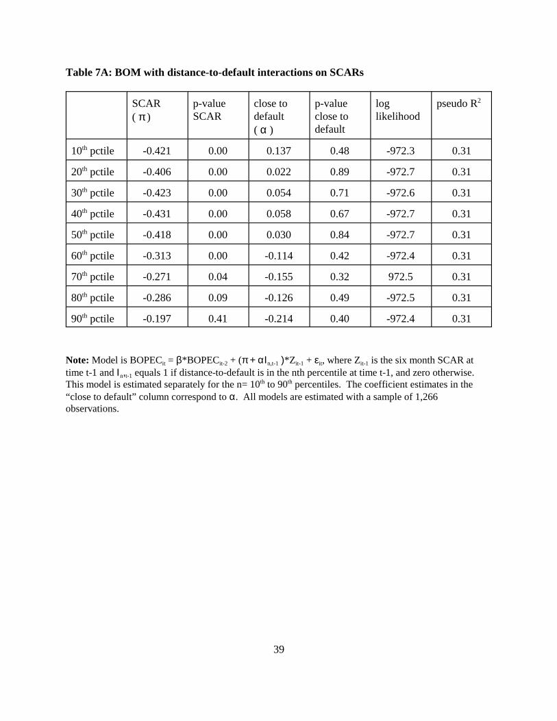
39

Table 7A: BOM with distance-to-default interactions on SCARs

SCAR( π )

p-valueSCAR

close todefault( α )

p-valueclose todefault

loglikelihood

pseudo R2

10th pctile -0.421 0.00 0.137 0.48 -972.3 0.31

20th pctile -0.406 0.00 0.022 0.89 -972.7 0.31

30th pctile -0.423 0.00 0.054 0.71 -972.6 0.31

40th pctile -0.431 0.00 0.058 0.67 -972.7 0.31

50th pctile -0.418 0.00 0.030 0.84 -972.7 0.31

60th pctile -0.313 0.00 -0.114 0.42 -972.4 0.31

70th pctile -0.271 0.04 -0.155 0.32 972.5 0.31

80th pctile -0.286 0.09 -0.126 0.49 -972.5 0.31

90th pctile -0.197 0.41 -0.214 0.40 -972.4 0.31

Note: Model is BOPECit = β*BOPECit-2 + (π + αΙn,t-1 )*Zit-1 + εit, where Zit-1 is the six month SCAR attime t-1 and Ιn,t-1 equals 1 if distance-to-default is in the nth percentile at time t-1, and zero otherwise. This model is estimated separately for the n= 10th to 90th percentiles. The coefficient estimates in the“close to default” column correspond to α. All models are estimated with a sample of 1,266observations.

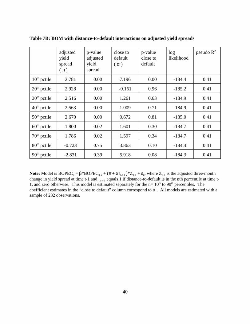
40

Table 7B: BOM with distance-to-default interactions on adjusted yield spreads

adjustedyieldspread( π )

p-valueadjustedyieldspread

close todefault( α )

p-valueclose todefault

loglikelihood

pseudo R2

10th pctile 2.781 0.00 7.196 0.00 -184.4 0.41

20th pctile 2.928 0.00 -0.161 0.96 -185.2 0.41

30th pctile 2.516 0.00 1.261 0.63 -184.9 0.41

40th pctile 2.563 0.00 1.009 0.71 -184.9 0.41

50th pctile 2.670 0.00 0.672 0.81 -185.0 0.41

60th pctile 1.800 0.02 1.601 0.30 -184.7 0.41

70th pctile 1.786 0.02 1.597 0.34 -184.7 0.41

80th pctile -0.723 0.75 3.863 0.10 -184.4 0.41

90th pctile -2.831 0.39 5.918 0.08 -184.3 0.41

Note: Model is BOPECit = β*BOPECit-2 + (π + αΙn,t-1 )*Zit-1 + εit, where Zit-1 is the adjusted three-monthchange in yield spread at time t-1 and Ιn,t-1 equals 1 if distance-to-default is in the nth percentile at time t-1, and zero otherwise. This model is estimated separately for the n= 10th to 90th percentiles. Thecoefficient estimates in the “close to default” column correspond to α . All models are estimated with asample of 282 observations.

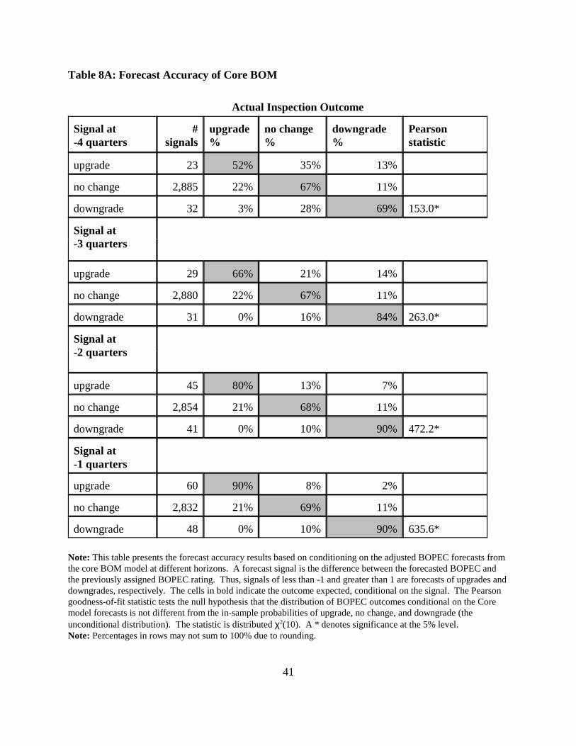
41

Table 8A: Forecast Accuracy of Core BOM

Actual Inspection Outcome

Signal at-4 quarters

#signals

upgrade%

no change%

downgrade%

Pearsonstatistic

upgrade 23 52% 35% 13%

no change 2,885 22% 67% 11%

downgrade 32 3% 28% 69% 153.0*

Signal at-3 quarters

upgrade 29 66% 21% 14%

no change 2,880 22% 67% 11%

downgrade 31 0% 16% 84% 263.0*

Signal at-2 quarters

upgrade 45 80% 13% 7%

no change 2,854 21% 68% 11%

downgrade 41 0% 10% 90% 472.2*

Signal at-1 quarters

upgrade 60 90% 8% 2%

no change 2,832 21% 69% 11%

downgrade 48 0% 10% 90% 635.6*

Note: This table presents the forecast accuracy results based on conditioning on the adjusted BOPEC forecasts fromthe core BOM model at different horizons. A forecast signal is the difference between the forecasted BOPEC andthe previously assigned BOPEC rating. Thus, signals of less than -1 and greater than 1 are forecasts of upgrades anddowngrades, respectively. The cells in bold indicate the outcome expected, conditional on the signal. The Pearsongoodness-of-fit statistic tests the null hypothesis that the distribution of BOPEC outcomes conditional on the Coremodel forecasts is not different from the in-sample probabilities of upgrade, no change, and downgrade (theunconditional distribution). The statistic is distributed χ2(10). A * denotes significance at the 5% level.Note: Percentages in rows may not sum to 100% due to rounding.

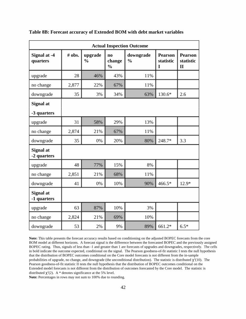
42

Table 8B: Forecast accuracy of Extended BOM with debt market variables

Actual Inspection Outcome

Signal at -4quarters

# obs. upgrade%

nochange%

downgrade%

PearsonstatisticI

PearsonstatisticII

upgrade 28 46% 43% 11%

no change 2,877 22% 67% 11%

downgrade 35 3% 34% 63% 130.6* 2.6

Signal at

-3 quarters

upgrade 31 58% 29% 13%

no change 2,874 21% 67% 11%

downgrade 35 0% 20% 80% 248.7* 3.3

Signal at-2 quarters

upgrade 48 77% 15% 8%

no change 2,851 21% 68% 11%

downgrade 41 0% 10% 90% 466.5* 12.9*

Signal at-1 quarters

upgrade 63 87% 10% 3%

no change 2,824 21% 69% 10%

downgrade 53 2% 9% 89% 661.2* 6.5*

Note: This table presents the forecast accuracy results based on conditioning on the adjusted BOPEC forecasts from the coreBOM model at different horizons. A forecast signal is the difference between the forecasted BOPEC and the previously assignedBOPEC rating. Thus, signals of less than -1 and greater than 1 are forecasts of upgrades and downgrades, respectively. The cellsin bold indicate the outcome expected, conditional on the signal. The Pearson goodness-of-fit statistic I tests the null hypothesisthat the distribution of BOPEC outcomes conditional on the Core model forecasts is not different from the in-sampleprobabilities of upgrade, no change, and downgrade (the unconditional distribution). The statistic is distributed χ2(10). ThePearson goodness-of-fit statistic II tests the null hypothesis that the distribution of BOPEC outcomes conditional on theExtended model forecasts is not different from the distribution of outcomes forecasted by the Core model. The statistic isdistributed χ2(2). A * denotes significance at the 5% level.Note: Percentages in rows may not sum to 100% due to rounding.

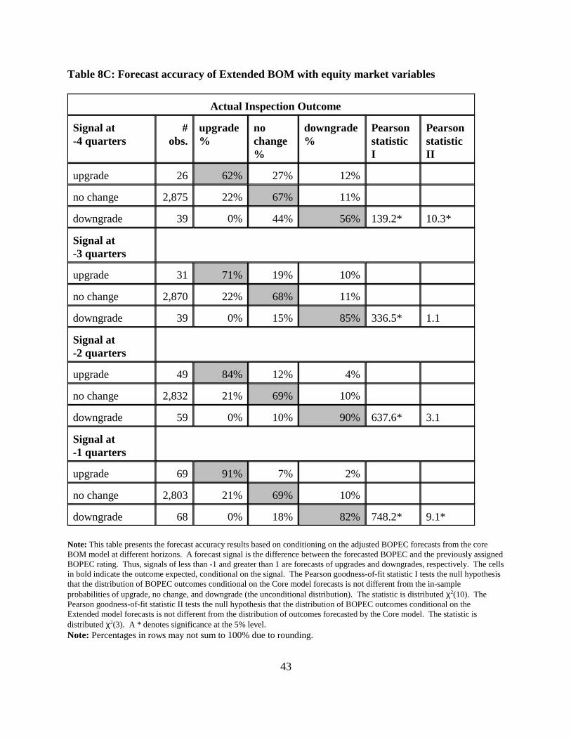
43

Table 8C: Forecast accuracy of Extended BOM with equity market variables

Actual Inspection Outcome

Signal at-4 quarters

#obs.

upgrade%

nochange%

downgrade%

PearsonstatisticI

PearsonstatisticII

upgrade 26 62% 27% 12%

no change 2,875 22% 67% 11%

downgrade 39 0% 44% 56% 139.2* 10.3*

Signal at-3 quarters

upgrade 31 71% 19% 10%

no change 2,870 22% 68% 11%

downgrade 39 0% 15% 85% 336.5* 1.1

Signal at-2 quarters

upgrade 49 84% 12% 4%

no change 2,832 21% 69% 10%

downgrade 59 0% 10% 90% 637.6* 3.1

Signal at-1 quarters

upgrade 69 91% 7% 2%

no change 2,803 21% 69% 10%

downgrade 68 0% 18% 82% 748.2* 9.1*

Note: This table presents the forecast accuracy results based on conditioning on the adjusted BOPEC forecasts from the coreBOM model at different horizons. A forecast signal is the difference between the forecasted BOPEC and the previously assignedBOPEC rating. Thus, signals of less than -1 and greater than 1 are forecasts of upgrades and downgrades, respectively. The cellsin bold indicate the outcome expected, conditional on the signal. The Pearson goodness-of-fit statistic I tests the null hypothesisthat the distribution of BOPEC outcomes conditional on the Core model forecasts is not different from the in-sampleprobabilities of upgrade, no change, and downgrade (the unconditional distribution). The statistic is distributed χ2(10). ThePearson goodness-of-fit statistic II tests the null hypothesis that the distribution of BOPEC outcomes conditional on theExtended model forecasts is not different from the distribution of outcomes forecasted by the Core model. The statistic isdistributed χ2(3). A * denotes significance at the 5% level.Note: Percentages in rows may not sum to 100% due to rounding.

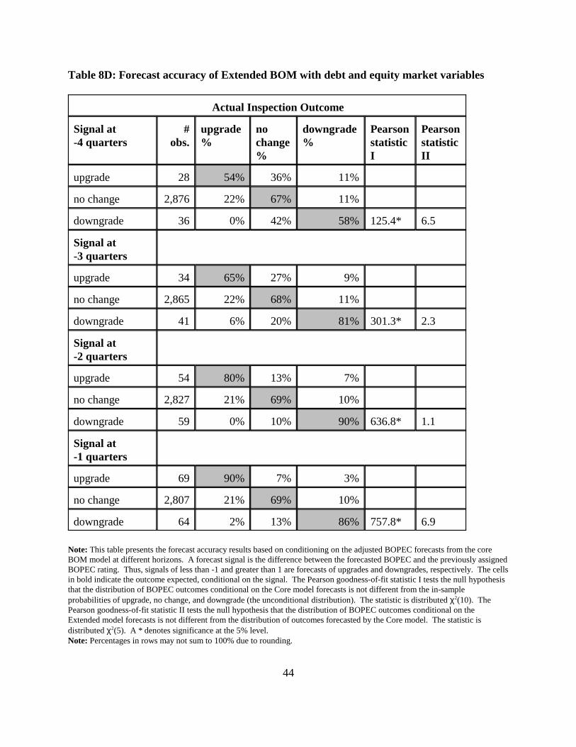
44

Table 8D: Forecast accuracy of Extended BOM with debt and equity market variables

Actual Inspection Outcome

Signal at-4 quarters

#obs.

upgrade%

nochange%

downgrade%

PearsonstatisticI

PearsonstatisticII

upgrade 28 54% 36% 11%

no change 2,876 22% 67% 11%

downgrade 36 0% 42% 58% 125.4* 6.5

Signal at-3 quarters

upgrade 34 65% 27% 9%

no change 2,865 22% 68% 11%

downgrade 41 6% 20% 81% 301.3* 2.3

Signal at-2 quarters

upgrade 54 80% 13% 7%

no change 2,827 21% 69% 10%

downgrade 59 0% 10% 90% 636.8* 1.1

Signal at-1 quarters

upgrade 69 90% 7% 3%

no change 2,807 21% 69% 10%

downgrade 64 2% 13% 86% 757.8* 6.9

Note: This table presents the forecast accuracy results based on conditioning on the adjusted BOPEC forecasts from the coreBOM model at different horizons. A forecast signal is the difference between the forecasted BOPEC and the previously assignedBOPEC rating. Thus, signals of less than -1 and greater than 1 are forecasts of upgrades and downgrades, respectively. The cellsin bold indicate the outcome expected, conditional on the signal. The Pearson goodness-of-fit statistic I tests the null hypothesisthat the distribution of BOPEC outcomes conditional on the Core model forecasts is not different from the in-sampleprobabilities of upgrade, no change, and downgrade (the unconditional distribution). The statistic is distributed χ2(10). ThePearson goodness-of-fit statistic II tests the null hypothesis that the distribution of BOPEC outcomes conditional on theExtended model forecasts is not different from the distribution of outcomes forecasted by the Core model. The statistic isdistributed χ2(5). A * denotes significance at the 5% level.Note: Percentages in rows may not sum to 100% due to rounding.

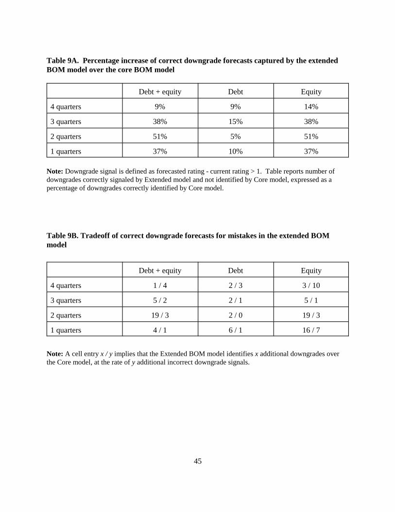
45

Table 9A. Percentage increase of correct downgrade forecasts captured by the extendedBOM model over the core BOM model

Debt + equity Debt Equity

4 quarters 9% 9% 14%

3 quarters 38% 15% 38%

2 quarters 51% 5% 51%

1 quarters 37% 10% 37%

Note: Downgrade signal is defined as forecasted rating - current rating > 1. Table reports number ofdowngrades correctly signaled by Extended model and not identified by Core model, expressed as apercentage of downgrades correctly identified by Core model.

Table 9B. Tradeoff of correct downgrade forecasts for mistakes in the extended BOMmodel

Debt + equity Debt Equity

4 quarters 1 / 4 2 / 3 3 / 10

3 quarters 5 / 2 2 / 1 5 / 1

2 quarters 19 / 3 2 / 0 19 / 3

1 quarters 4 / 1 6 / 1 16 / 7

Note: A cell entry x / y implies that the Extended BOM model identifies x additional downgrades overthe Core model, at the rate of y additional incorrect downgrade signals.