Embed Size (px)
Citation preview

1
2
Using Synthetic Population Generation to Replace Sample and 3 Expansion Weights in Household Surveys for Small Area 4
Estimation of Population Parameters 5
6 Konstadinos G. Goulias 7
GeoTrans, UCSB 8
Srinath K. Ravulaparthy 9
GeoTrans, UCSB 10
Karthik Konduri 11
University of Connecticut 12
Ram M. Pendyala 13
Arizona State University 14
15 16 17
18
July 4, 2013 19
20
Paper Submitted for Presentation at the 93rd Annual Meeting 21
of the Transportation Research Board 22
23
24
25

1
Using Synthetic Population Generation to Replace Sample and 1 Expansion Weights in Household Surveys for Small Area 2
Estimation of Population Parameters 3 4
5
6
7
Abstract: In this paper we illustrate the use of synthetic population generation 8
methods to replace sample weights and expansion weights in household travel surveys. 9
We use a combination of exogenous (US Census) and endogenous (the survey) data as 10
the informants and in essence transfer information from the county level sample to the 11
tracts. The method is based on PopGen and is applied to the newly collected data in the 12
California Household Travel Survey (CHTS). An illustration of using traditional 13
sampling and expansion weights and synthetic population generation is illustrated at the 14
tract level. We show synthetic population methods are able to recreate the entire spatial 15
distribution of households and persons in small areas, recreate the variation that is lost 16
when sampling and possibly mimics the variation in the real population, enable 17
transferability without having to develop complicated methods and fills spatial gaps in 18
data collection, produce a large database that is ready to be used in activity 19
microsimulation, provides as byproducts sample and expansion weights; and offers the 20
possibility to perform resampling for model estimation. However, these claims require 21
further testing and verification. 22
23
24
Paper Submitted for Presentation at the 93rd Annual Meeting 25
of the Transportation Research Board 26
27

2
1
INTRODUCTION 2 3
Sample weights (often claimed to be the inverse probabilities of selection for each 4
observation) aim at reshaping the sample to make it look like a simple random draw of 5
the total population. In this way descriptive statistics from the reshaped sample produce 6
"more" accurate population estimates than the original unweighted sample. The survey 7
design and associated statistical analysis literature offers a variety of solutions to perform 8
this reshaping to counter a variety of design complications but also mistakes in data 9
collection. In post survey data collection we face mainly two options for reshaping the 10
sample distributions of values to mimic the population and they are: a) develop weights 11
for unit of data (household, person, activity, trip); and b) develop regression models that 12
account for external and internal stratification and self-selection biases. The first method 13
requires knowledge about the distribution of values of population parameters and careful 14
monitoring of survey stages to detect self-selection and its determinants. The second 15
method requires model specifications that include variables controlling the process of 16
sample selection. Both approaches can become extremely complex when one needs to 17
estimate not only the population means of parameters but also their variances and the 18
relationships among different variables (Chung and Goulias, 1995, Gelman, 2007, 19
Dumouchel and Duncan, 1983, Friedman, 2013, Gelman and Carlin, 2002, Kish, 1992, 20
Lu and Gelman, 2003, Ma and Goulias, 1997, Pendyala et al., 1993, Pfeffermann, 1993, 21
Solon et al., 2013, Winship and Radbill, 1994). In small area estimation with small area 22
in this case intended as geographic area (statisticians use the word to also mean small 23
segments of the population, which leads to similar issues) added complications include 24
lack of local external to the survey data, cross-tabulation of variables that have many 25
structural zeros, very few sample survey observations, and methods that are designed 26
only for ideal situations (Chambers and Tzavidis, 2006, Datta et al., 2011, Fay and 27
Herriott, 1979, Jiang et al., 2011, Li and Lahiri, 2010, Molina and Rao, 2010, Pfefferman 28
and Sverchkov, 2007, Sinha and Rao, 2009, Tzavidis et al., 2010, You et al., 2012). 29
30

3
The third possibility of developing sample weights is to employ methods from synthetic 1
population generation (Beckman et al., 1996, Chung and Goulias, 1997, Greaves and 2
Stopher, 2000, Bowman, 2004 and references therein, Frick and Axhausen, 2004, Auld et 3
al., 2009, Guo and Bhat, 2007). This is a method that is gaining acceptance in travel 4
demand forecasting, it is a related method to multiple imputation (Rubin, 1987, 1996) and 5
data augmentation (Schafer, 2010), it is feasible at any level of US Census geographic 6
aggregation (block, blockgroup, tracts, traffic analysis zone), and attacks the problem of 7
survey weighting in a way that solves multiple problems including transferability. 8
However, testing and experimentation with this method as a survey reshaping tool is not 9
widespread and very few authors report their experience (Greaves and Stopher, 2000) but 10
none in attempting small area estimation. In this paper we illustrate the method using 11
data from the California Household Travel Survey that was completed in March 2013, 12
show preliminary results and discuss next steps. 13
14
The California Household Travel Survey (CHTS) sampled households from different 15
segments of the population with different probabilities. This was done to obtain more 16
precise information on the smaller subgroups in the population and to minimize the 17
chance of missing a few population segments that are difficult to reach and interview. 18
CHTS is used to calculate descriptive statistics that aim at accurately measuring the true 19
values of parameters of interest in the population at a variety of geographic scales. The 20
second type of analysis is the creation of behavioral models that contain relationships 21
among variables of interest (e.g., number of cars in a household as a function of 22
household income). The statistical literature claims that sometimes weights are needed, 23
other times they are not influential, and some other times weights could even introduce 24
bias in estimates. Unfortunately, when this happens we are forced to develop 25
complicated weights and perform weighted and unweighted estimation to study the 26
sensitivity of our models to weight application. If synthetic population is used for small 27
area estimation, it makes more theoretical and practical sense to use this population for 28
model estimation too. This paper clarifies some of these issues and provides options for 29
weight creation. It also offers an illustration of the issues in small area estimation with 30

4
examples of specific tracts in California. 1
In the next section, we describe the data collection and sample selection steps. This is 2
followed with a discussion of weight creation options and an illustration of small area 3
estimation issues as well as the solution. The paper concludes with a summary and next 4
steps for further analysis. 5
6
The 2010 CALIFORNIA HOUSEHOLD TRAVEL SURVEY 7 8
The 2010 California Household Travel Survey is designed with the new California policy 9
framework in mind, taking into account the possible use of new technologies, as its 10
Steering Committee clearly defines in the following paragraph. “The purpose of the 11
CHTS is to update the statewide database of household socioeconomic and travel 12
behavior used to estimate, model and forecast travel throughout the State. Traditionally, 13
the CHTS has provided multi-modal survey information to monitor, evaluate and make 14
informed decisions regarding the State transportation system. The 2010 CHTS will be 15
conducted to provide regional trip activities and inter-regional long-distance trips that 16
will be used for the statewide model and regional travel models. This data will address 17
both weekday and weekend travel. The CHTS will be used for the Statewide Travel 18
Demand Model Framework (STDMF) to develop the information for the 2020 and 2035 19
GHG emission rate analyses, calibrate on-road fuel economy and fuel use, and enable 20
the State to comply with Senate Bill 391 (SB 391) implementation. The CHTS data will 21
also be used to develop and calibrate regional travel demand models to forecast the 2020 22
and 2035 Greenhouse Gas (GHG) emission rates and enable Senate Bill 375 (SB 375) 23
implementation and other emerging modeling needs.” 24
25
One common objective for the data collected in this household travel survey is to develop 26
a variety of newly formulated travel demand forecasting systems throughout the state and 27
integrate land use policies with transportation policies. Very important for regional 28
agencies is the provision of suitable data that inform a variety of new model development 29
including the Activity-based models (ABM) and their integration with land use models at 30

5
the State level and for each of the four major Metropolitan Planning Organizations 1
(MPO). It is also the source of data for the many refinements of older four-step models 2
and activity-based models in smaller MPOs and serves as the main source of data for 3
behavioral model building, estimation of modules in other sustainability assessment tools, 4
and the creation of simplified land use transportation models. Moreover, added details 5
about car ownership and car type of households will be needed to develop a new set of 6
models to more accurately estimate emissions of pollutants at unprecedented levels of 7
temporal and spatial resolutions. 8
9
The CHTS databases (data collected by NUSTATS for the entire state and Abt-SRBI 10
added sample for Southern California Association of Governments - SCAG) include 11
information about the household composition and facilities available, person 12
characteristics of the persons in each household, and a single day place-based activity and 13
travel diary. The first component is called the recruitment component and the second 14
(diary) the retrieval. In addition, a set of satellite type of surveys (a subset of households 15
invited to participate in additional survey components) were also designed and 16
administered to gain insights about the use of the transportation system (e.g., wearable 17
GPS, GPS and OBD for cars) and to potentially complement and rectify travel 18
information. Moreover, a long distance (for trips longer than 50 miles) extending for up 19
to 8 weeks before the diary day was also designed and administered. For the SCAG 20
region Abt-SRBI designed and administered an add-on augment satellite survey 21
containing questions that are specifically needed for model building at SCAG. The CHTS 22
(NUSTATS and Abt-SRBI) sample selection is a combination of exogenously stratified 23
random and convenience (see NUSTATS Final Report, 2013). This creates the need to 24
identify ways that sample data can be "adjusted" to represent the resident population. 25
26
We define as "Universe of Addresses" all the addresses that are found within a tract. 27
Similarly we define as "Resident Households" all the households that live within a tract. 28
A sample of addresses is a portion of the Universe of addresses and a sample of 29
households is a portion of the resident households. The number of addresses in a tract 30
should be higher than the number of households. For example, in Los Angeles County the 31
6
following three tracts were delivered by a vendor of addresses from which samples were 1
selected. The three tracts show that tract number 06037481101 has 1445 addresses, tract 2
number 06037481102 has 1474 addresses and tract number 06037481103 has 1536 3
addresses. If in CHTS the vendor randomly selected from each tract 10 addresses, for 4
tract number 06037481101 the probability of selection would be 10/1445 and the weight 5
of each address 1445/10 = 144.5. In this way every address selected represents 144.5 6
addresses in that tract. If the same vendor selected another 5 addresses for Abt-SRBI, the 7
probability of selection would be (10+5)/1445 and the weight would be 1445/15 and 8
every selected address representing 96.333 addresses. One could think to apply this 9
weight to the households in CHTS in each tract but this does not apply to all selected 10
households when other sample frames are added. 11
12
Section 3.2.1 (NUSTATS, 2013) states: 13
"An Address-‐based sampling frame approach was used. An Address-‐based sample is a random 14 sample of all residential addresses that receive U.S. Mail delivery. Its main advantage is its reach 15 into population groups that typically participate at lower-‐than-‐average levels, largely due to 16 coverage bias (such as households with no phones or cell-‐phone only households). For efficiency 17 of data collection, NuStats matched addresses to telephone numbers that had a listed name of 18 the household appended to the sampled mailing addresses. This sampling frame ensured 19 coverage of all types of households irrespective of their telephone ownership status, including 20 households with no telephones (estimated at less than 3% of households in the U.S.). In order to 21 better target the hard-‐to-‐reach groups, the address-‐based sample were supplemented with 22 samples drawn from the listed residential frame that included listed telephone numbers from 23 working blocks of numbers in the United States for which the name and address associated with 24 the telephone number were known. The “targeted” Listed Residential sample, as available from 25 the sampling vendor, included low-‐income listed sample, large-‐household listed sample, young 26 population sample, and Spanish-‐surname sample (to name a few). As expected, this sample was 27 used to further strengthen the coverage of hard-‐to-‐reach households. The advantage of drawing 28 sample from this frame is its efficiency in conducting the survey effort—being able to directly 29 reach the hard-‐to-‐reach households and secure their participation in the survey in a direct and 30 active approach. Both address and listed residential samples were procured from the sample 31 provider – Marketing Systems Group (MSG) based in Fort Washington, PA. The survey 32 population was representative of all households residing in the 58 counties in California. 33 According to 2010 Census data, the survey universe comprised 12,577,498 households. Table 34 3.2.3.1 provides the distribution of households by counties and by MPO/RTPA. As shown in the 35 table, 83% resided in four MPO regions (spread over 22 counties) – 46% in SCAG, 21% in MTC, 36 9% in SANDAG, and 7% in SACOG. The remaining 17% households reside in 36 counties in 37 California." 38
39
Moreover, additional rules were used to identify tracts with households of interest (e.g., 40
7
most likely hard to reach). Applying a naive weighting procedure would lead to biases 1
because the final list of households with complete data are the result of many 2
intermediate events from their address selection to final data delivery. A few of these 3
events include inability to contact, refusing to participate and so forth and their outcome 4
is a function of the characteristics of the household and the person responding to the 5
survey as well as the ability of the data collection company to convince respondents to 6
participate and the different skills of the company's interviewers. It is usually not feasible 7
to know the characteristics of these persons for such a large survey and this increases the 8
uncertainty about self-selection of the final set of respondents in the recruitment stage. 9
From many other studies we know that self-selection is usually systematic, which means 10
the survey participants are systematically different (in their observed and unobserved 11
characteristics) than the non participants and obviously different from the population of 12
interest. For example, we knew from the pilot survey in Fall 2011 that CHTS is 13
attracting a sample that does not represent the age and gender distribution of California. 14
15
A separate issue is our uncertainty about the population characteristics at the tract level. 16
We should keep in mind that ACS (Table 2, shows data from the three tracts mentioned 17
above that are 4811.01, .02. and .03) is a survey and because of this it also carries an 18
error with its estimates and as can be seen from Table 1 this error is substantial (see the 19
third column of each tract of Table 1). However, the relative "closeness" between the 20
number of addresses the vendor reports and number of households is noteworthy. For 21
example, in tract 4811.01 we see in ACS 1425 households and in the sampling frame 22
used to select sample units we find 1450 addresses. The other two tracts show larger 23
differences. Presumably this is due to housing units with unique address that are not 24
occupied by households and possible errors in the sample frame and ACS data. 25
26
Independently of data errors about the statistical universe these differences show that 27
addresses and households are not only conceptually different but also numerically 28
different in each tract in a differential way (i.e., for some tracts we have larger differences 29
and others we have smaller differences). This is the main reason we need to include at 30
least two stages in weight creation. The first stage estimates the probability of selection 31

8
for each address (the inverse of which is the sample weight) and the second stage aims to 1
adjust the household and person probability of selection based on the information 2
available externally such as ACS or the control totals developed by SCAG's demographic 3
prediction procedures. 4
5
Table 1. The US Census American Community Survey (2007-2011). 6
7 8 The combined weights will give the proper "importance" for each household. In this way 9
estimation of descriptive statistics represents the resident population and behavioral 10
models are based on data without major biases. In addition, separate weights can be 11
developed to function as expansion weights reproducing the total numbers we obtain 12
from the US Census. For practical purposes we will name sampling weights the 13
multipliers of each unit/record in CHTS that give differential importance to each record 14
to account for unequal probability of selection and expansion weights the weights that 15
reproduce the entire population. Multiplying each record by its sampling weight(s) 16
maintains the sample size and it is the right weight to use for model estimation, 17
otherwise, all statistics are inflated in an artificial way. 18
19
Stages of Sample Selection 20 21
In sample selection we should distinguish between the selection done by the analysts and 22
the selection done by each household to participate in the survey (self-selection). The 23

9
stages below describe each stage and the sample selection steps. 1
2
First Stage: Selection by address and listed phone numbers 3 4 Although the original plan for CHTS was to recruit households from an exclusively 5
address based sampling frame (called ABS in the NUSTATS report), in early 2012 a 6
second sampling frame was added that is based on listed telephone numbers (to the best 7
of our understanding). Moreover, NUSTATS performed an active sampling redesign as 8
the survey administration was progressing. This was considered necessary because 9
response rates were extremely low. However, this creates a major problem in estimating 10
probability of selection (and its inverse that is usually the sampling weight) because the 11
number of observations does not have a well defined universe from which a sample unit 12
is selected. In fact, there are a few complications distancing the CHTS sample from a 13
random sample. During the step of selecting addresses analysts, instead of drawing one 14
address from the total number of addresses in a tract, select a household by a combination 15
of criteria that includes the address in a tract, the tract within a geographic stratum, and 16
four main household characteristics treated as targets that are Hispanic last name, low 17
income (<$25,000), large household (household size >3), young household (Age<25), 18
and for some transit classified tracts added sampling to increase transit use in the sample 19
as well as zero vehicle households. In addition, other segments were added from special 20
recruitment (see Table 6.4.1, NUSTATS, 2013). This complicates the process and the 21
uncertainty about the value of the denominator of the calculation of probability of 22
selection. Moreover, after households were selected for the first contact, they refused or 23
were not available for a variety of reasons to participate. Non-responding households are 24
also systematically different than responding households introducing another incidence of 25
self-selection bias in CHTS. 26
27 28
Second Stage: Retrieval Management 29 30 Based on the NUSTATS final report (section 4.2.13): 31

10
"Sample management for retrieval was an on-‐going and hands on task that often times required 1 supervisory and management staff to discuss sample segments or even specific households on 2 the best approach to finalize the household. Some of the considerations taken into account 3 included whether the household had been called during the day of the week and time of the day 4 when the recruitment interview took place, whether calls had been spread out across times of 5 the day and days of the week, whether any or too many messages had been left, or whether the 6 household needed to be finalized as non-‐completed and needed to be replaced. The Strata and 7 Quotas definition module in VOXCO allowed NuStats to manage subsets of the sample and to 8 open or close access to any stratum or subset as needed. It also allowed NuStats to apply quotas 9 or ceilings to control the maximum number of completed interviews by stratum, and the rate at 10 which they were attained. This module was used for tracking goals and in sample management 11 by assisting in the release or withholding of specific sample segments. Many of the sample 12 management activities already described were made possible by a specific strata definition that 13 existed in the Quota Management module. The starting point of making this sample control tool 14 work was to specify a set of criteria or strata, upon which sample controls or quotas were to be 15 applied. For the CHTS, quotas also were used to monitor household distribution across travel 16 days to obtain a proportional distribution of days of the week and across weeks and months 17 during the full year of data collection. There were situations in which there was a need to 18 regulate or balance the rate at which a group of strata were filled during the course of the 19 project. To achieve this, a probability or weight was assigned to a lagging stratum, so that the 20 system would increase the rate by which sample from that strata was released. This process was 21 critical for achieving goals on time, for example when the deadline for closing out a wearable 22 MTC scheduling date was approaching, adding a weight to the wearable MTC sample ensured 23 more of this sample was called to increase the chances to meet the goal on time." 24 25 The paragraph above shows that NUSTATS for pragmatic considerations combined 26
probability sample selection with non-probability (quota) sample selection introducing 27
biases by aiming at meeting quotas and violating the probability-based selection of 28
sample units. Solutions for this type of process exist and a simple "raking" weight 29
creation may mask biases but may also be our only option. In addition, households that 30
agree to participate in the diary portion (called complete households in CHTS) are 31
systematically different than the households selected in the first stage. The options 32
presented in the next section aim at rectifying these biases. Under an ideal weight 33
creation scenario we should develop weights for every decision point of sample selection. 34
This requires a very carefully and meticulously documented sample monitoring process 35
that in parallel also monitors the corresponding population characteristics. For example 36
for each tract we need to have reports of the number of addresses and the number of 37
listed numbers by each group from which a sample unit (address and household) was 38
selected. In addition, the population characteristics when they are known are also not 39
known with certainty (e.g., ACS is a survey with its own set of data collection errors and 40

11
cross-classification of household income by ethnicity and household size of the resident 1
population is not available not even at the tract level). 2
3
There are, however, alternate options from a more pragmatic viewpoint that on the one 4
hand rectify some of the survey sample biases and on the other hand offer a way to 5
combine data from the two data collection companies as well as the two main sources of 6
information: the CHTS sample and ACS. These options have similarities with the 7
method used by NUSTATS (two stage address/listed and raking) but with the added 8
flexibility to employ many additional variables as external controls and to use different 9
geographic subdivisions to match the Traffic Analysis Zones of MPOs while at the same 10
time using a combined database of the NUSTATS and Abt-SRBI core data. In summary, 11
there are three main reasons to create sample weights (and expansion weights) and 12
reshape the sample to resemble the residents population and they are: 13
14
• Weights to represent addresses in each tract 15
• Weights to adjust household and person characteristics of each tract 16
• Weights to counter selectivity bias between recruitment and retrieval 17
The options presented below aim at addressing each of these three reasons. All options 18
below require to first merge the household data from NUSTATS and Abt-SRBI into one 19
database that is harmonized. The same should be done for the person data. We also 20
distinguish below between complete and incomplete households. The incomplete 21
households are the households for which we do not have all the information about 22
activity and travel. 23
24 Before listing the options a few words about the PopGen population synthesis are in 25
order. To create a synthetic population PopGen uses two main sources of information: a) 26
a sample that functions as "seed" to provide records that can be repeatedly used as the 27
"donor" records to replicate and produce the final population; and b) target distributions 28
of variables that function as controls (constraints). The algorithm first creates the 29
equivalent of a contingency table of key variables at the household level (e.g., household 30
size, household income) and the person level (e.g., age categories, gender). These are 31

12
provided by the seed survey sample. Then, "weights" are developed that reproduce 1
correctly the target distributions of the control variables. Then, a routine randomly 2
selects donor households that satisfy these weights and allocates them to a geographic 3
unit keeping track of how many times each donor is selected. The software preserves the 4
original donor identification record number allowing to carry over all its characteristics 5
(including behavioral variables). 6
7
8 Option A. Merge all the complete data and use the final complete households and 9
persons from NUSTATS and Abt-SRBI. Develop weights at the TAZ/Tract level using 10
MPO provided sociodemographic estimates (e.g., SCAG has a complex process of 11
computing these together with local jurisdictions) employing PopGen. These will be 12
expansion weights because PopGen creates a synthetic population (see Ye et al., 2009). 13
Use as descriptive statistics the characteristics of the synthetic population. We can 14
distinguish between two slightly variants: Option A.1- Use as seed cross-tabulations in 15
SCAG-CHTS and Option A.2 - Use as seed the address weighted cross-tabulations in 16
SCAG-CHTS. 17
18
Option B. First merge all the complete data and use the final complete households and 19
persons from NUSTATS and Abt-SRBI. Then, develop a first set of weights for US 20
Census tract residence using the data provided by Abt-SRBI. Finally, Use PopGEN as a 21
raking algorithm and as seed the weighted cross-tabulations from second step above. 22
23
Option C. First merge all the data including the partially complete to form one household 24
level and one person level database. Then, develop a first set of weights for tract 25
residence using the data provided by Abt-SRBI. After this step create a probability 26
model with dependent variable taking the value of 1 if the household responded to the 27
diary portion and 0 otherwise. Use as explanatory variables in this nonlinear regression 28
variables that explain willingness to participate and these can include location of the 29
household. Take the inverse of the probability and use it as household sample weight. 30
Finally, use PopGen as the raking procedure with seed the weighted households with 31

13
weights from the second and third steps. 1
2
A comparison among Options A, B, and C will show if we need the more labor intensive 3
B and C options. In the next section an example of Option A.1 is offered to illustrate 4
PopGen's ability to reproduce external data. 5
6
Illustration of Option A.1 7 8
As a proof of concept in this section we report findings from a small pilot project that we 9
recently completed to illustrate the ability of PopGen to function as sample rectifier in 10
small geographic areas. We selected six tracts in Santa Barbara county and San Louis 11
Obispo county. This was done for two reasons: a) we are familiar with the area; and b) 12
NUSTATS collected a very small sample for these two counties due to 13
administrative/management reasons. We will use these six tracts as case studies for 14
which we will synthetically generate the households and persons they include as residents 15
and their characteristics. 16
17
In this pilot experiment we use as "seed" database the records of 1,282 (in the database) 18
and 1,023 (in the final report of NUSTATS) households that participate in CHTS from 19
the Counties of San Louis Obispo and Santa Barbara. For control distributions we use 20
the ACS 2006-2010 reported data for each tract in this same region. The four control 21
variables are: Household size (with values 1, 2, 3, 4 or more), household income (with 22
categories Less than $9,999, $10,000 - $24,999, $25,000 – $34,999, $35,000- $49,999, $50,000 - 23
$74,999, $75,000-$99,999, $100,000-$149,999, $150,000 - $199,999, $200,000 or above), age 24
(25 or below, >25 and <40, >=40 and <50, >=50 and <65, and >=65 and above), and 25
gender (male and female). It is the combination of the categories of these variables that 26
PopGen is attempting to replicate (finding how many combinations correspond to the 27
population that generated the control totals of the data used as targets). This is a very old 28
problem in statistics that is solved with the Iterative Proportional Fitting (IPF) algorithm 29
and in modeling software the Expectation - Maximization (EM) algorithm. Similar 30
algorithms are used in the derivation of weights in the procedure known as "raking." 31
14
PopGen has a very robust algorithm with different options (PopGen 1.1, 2011, Ye et al., 1
2009, Bar-Gera et al., 2009). NUSTATS in its final deliverable also used a raking 2
algorithm to adjust weights and control for distributions at larger geographical areas than 3
tracts. 4
5
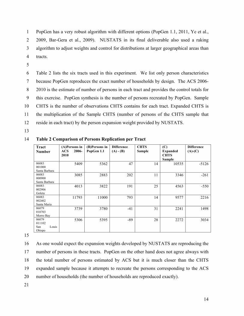
Table 2 lists the six tracts used in this experiment. We list only person characteristics 6
because PopGen reproduces the exact number of households by design. The ACS 2006-7
2010 is the estimate of number of persons in each tract and provides the control totals for 8
this exercise. PopGen synthesis is the number of persons recreated by PopGen. Sample 9
CHTS is the number of observations CHTS contains for each tract. Expanded CHTS is 10
the multiplication of the Sample CHTS (number of persons of the CHTS sample that 11
reside in each tract) by the person expansion weight provided by NUSTATS. 12
13
Table 2 Comparison of Persons Replication per Tract 14 Tract Number
(A)Persons in ACS 2006-2010
(B)Persons in PopGen 1.1
Difference (A) - (B)
CHTS Sample
(C) Expanded CHTS Sample
Difference (A)-(C)
06083 001000 Santa Barbara
5409 5362 47 14 10535 -5126
06083 000900 Santa Barbara
3085 2883 202 11 3346 -261
06083 002906 Goleta
4013 3822 191 25 4563 -550
06083 002402 Santa Maria
11793 11000 793 14 9577 2216
06079 010703 Morro Bay
3739 3780 -41 31 2241 1498
06079 011102 San Louis Obispo
5306 5395 -89 28 2272 3034
15
As one would expect the expansion weights developed by NUSTATS are reproducing the 16
number of persons in these tracts. PopGen on the other hand does not agree always with 17
the total number of persons estimated by ACS but it is much closer than the CHTS 18
expanded sample because it attempts to recreate the persons corresponding to the ACS 19
number of households (the number of households are reproduced exactly). 20
21

15
The second part of the illustration (Table 3) examines the age distribution replication by 1
CHTS (unweighted and weighted sample) and the generated synthetic population by 2
PopGen. We report only the person characteristics of Tract number 06079011102. 3
4 5 Table 3 Age Distribution within Tract 06079011102 6 ACS 2006-2010 PopGen CHTS Sample CHTS Expanded AGE Frequency Percent Frequency Percent Frequency Percent Frequency Percent <=25 2383 44.9 2426 45.0 4 14.3 369 16.2 >25 & <40 1273 23.9 1299 24.1 3 10.7 372 16.4
>=40 & <50 490 9.23 531 9.8 4 14.3 266 11.7
>=50 & <65 799 15.05 787 14.6 14 50.0 897 39.5
>=65 361 6.80 352 6.5 3 10.7 368 16.2 Total 5306 100.0 5395 100.0 28 100.0 2272 100.0 7 The age distribution produced by PopGen closely resembles the ACS age distribution 8
because it uses it as target. The age distribution of the weight expanded CHTS is not 9
reproducing ACS at this level of geography because it was not intended for this purpose 10
and used a different geography to derive sample and expansion weights. This shows that 11
Metropolitan Planning Organizations in California should not use these weights if they 12
need to perform data analysis and model estimation at the tract level (this is the level that 13
Traffic Analysis Zones are often defined). 14
15
It should also be noted that PopGen before creating a synthetic population creates 16
weights for each combination of control variables. This translates into weights for each 17
unit in the sample used as seed. When the sample used as seed is the CHTS survey, 18
PopGen in essence produces the equivalent of raking weights for CHTS balancing the 19
information at the household level with the information at the person level. MPOs can 20
use these weights to perform weighted sample descriptive analysis at higher level of 21
geography (e.g., the county level). 22
23
An additional benefit in using synthetic population generation with seed information 24
from a survey is also our ability to "carry over" other variables that were not used in 25

16
developing weights and marginal control total targets. For example, we use the 1
information in the synthetic population to estimate the number of trips per person per day 2
at each tract analyzed here. Table 4 shows this estimate for each tract of Table 2. 3
4
Table 4 Estimates of Daily Trips per Person 5
Tract Number
Daily Trips/person
Synthetic Persons
Std. Deviation
In CHTS Respon-dents
Weighted CHTS
900 3.39 2882 2.905 3.64 11 3.57
1000 3.50 5360 2.995 3.93 14 3.27
2402 3.48 10983 3.054 2.21 14 2.12
2906 3.57 3801 3.029 2.75 24 2.55
10703 3.40 3779 2.908 3.61 31 3.18
11102 3.99 5393 3.717 4.29 28 4.07
Total
32198
122
6
The average number of daily unweighted person trips in CHTS are: in Santa Barbara 3.43 7
(sd = 2.96) by 1044 persons and in San Louis Obispo are 3.20 (sd = 2.83) trips by 1898 8
persons. When we apply the NUSTATS sampling weights for Santa Barbara we get 3.31 9
(sd = 2.92) trips by 1201 persons and the average number of trips in San Louis Obispo is 10
3.18 (sd=2.78) trips by 797 persons. The synthetic population performed an averaging of 11
the values derived from the small samples borrowing information from the entire county. 12
On the other hand weighted CHTS amplifies the already skewed sample of each tract (see 13
Tracts 2402 and 2906). 14
15
Regression Models and Sample Weights 16 17
The majority of the models used in activity-based and trip-based approaches to travel 18
demand forecasting are based on regression methods (this includes the discrete choice 19
models). In model estimation as mentioned in the introduction we are aware of the need 20
and risks of using weights. In model estimation based on data that are not collected in a 21
completely random way we have two schools of thought: a) regression models do not 22
need weighted sample if one includes all the variables that were used to stratify or 23
otherwise bias the sample; and b) regression models should use weights to account for 24
17
data collection that is not completely equiprobability in sample selection. Therefore, for 1
model estimation we can use specifications that include as explanatory variables place of 2
residence, household income, age of respondents and age of householder, ethnicity to 3
account for sample selection used by NUSTATS (these are also the sample weight 4
creation by raking dimensions). If an MPO adheres to the first school of thought and 5
uses sampling weights in regression model estimation, the weights produced by PopGen 6
and attached to each household and person used in the seed could be employed. 7
Alternatively, models can be enriched in their estimation with an array of variables that 8
account for sample selection. However, there is a third method that we believe is 9
superior to these two. 10
11
After a region-wide synthetic population is created using as seed the CHTS data, multiple 12
random samples can be extracted. Then, for model estimation we can use these random 13
samples from this synthetic population. A repeated resampling from the synthetic 14
population and estimation of models will provide an empirical test of the variability in 15
regression coefficients. It is expected that different samples will lead to similar 16
coefficients. However, as in many applications of this type it is always a good idea to 17
include in the explanatory variables as many indicators as possible that can capture the 18
selectivity bias in the survey design. For example, household characteristics (size and 19
age composition), household income, and ethnicity will control for the initial selection of 20
households. A variety of location indicators will also account for the county of residence 21
stratification. For example, in SimAGENT using as explanatory variables the 22
accessibility indicators that were developed at fine spatial resolution will eliminate the 23
need to account for county of residence. 24
25
18
1
SUMMARY 2 3 Considerable complications emerging from extremely low response rates and the need to 4
avoid major disasters in data collection create the need to develop sampling weights that 5
are based on only partial information with unknown precision and unusable small area 6
estimation of population parameters. In this paper we illustrate the use of synthetic 7
population generation methods to fill the gap. We use a combination of exogenous (US 8
Census) and endogenous (CHTS database) as the informants and in essence transfer 9
information from the county level sample to the tracts. Three possible options are also 10
presented as variants of the use of synthetic population as the core methodology. There 11
are many advantages doing this because a synthetic population: 12
13
a) recreates the entire spatial distribution of households and persons in small areas; 14
b) recreates the variation that is lost when sampling and possibly mimics the variation in 15
the real population; 16
c) enables transferability without having to develop complicated methods and fills spatial 17
gaps in data collection; 18
d) produces a large database that is ready to be used in activity microsimulation; 19
e) provides as byproducts sample and expansion weights; and 20
f) offers the possibility to perform resampling for model estimation. 21
22
Additional testing and experimentation is required, however, to provide guidelines on the 23
use of the methods here and to make comparisons with alternate procedures. 24
25
26
Acknowledgments 27 28 SCAG and BMC provided support for the latest development of PopGen. CALTRANS, 29 SCAG, MTC, CEC and other agencies provided funding for data collection in CHTS. 30 Funding for this paper was also provided by UCTC and UC MRPI on Sustainable 31 Transportation. This paper does not constitute policy of any government agency. 32 33 34

19
REFERENCES/BIBLIOGRAPHY 1
Auld, J., Mohammadian, A., Wies, K., 2009. Population synthesis with sub-region-level 2 control variable aggregation. ASCE Journal of Transportation Engineering 135 (9), 3 632–639. 4
Bar-Gera H., KC Konduri, B Sana, X Ye, RM Pendyala (2009) Estimating survey 5 weights with multiple constraints using entropy optimization methods. Paper presented 6 at Transportation Research Board 88th Annual Meeting and included in the CD ROM 7 proceedings. 8
Beckman, R.J., Baggerly, K.A., McKay, M.D., 1996. Creating synthetic baseline 9 populations. Transportation Research, Part A 30, 415–429. 10
Bowman J (2004) A Comparison of Population Synthesizers Used in Microsimulation 11 Models of Activity and Travel Demand. Working Paper. <http:// jbowman.net/> 12 (Accessed 07/03/2013). 13
Chambers, R. and Tzavidis, N. (2006). M-quantile models for small area estimation. 14 Biometrika, 73, pp. 597-604. 15
Chung, J. and K. G. Goulias (1995) Sample selection bias with multiple selection rules: 16 An application with residential relocation, attrition, and activity participation in the 17 Puget Sound transportation panel. Transportation Research Record, 1493, pp. 128-135. 18
Chung, J. and K.G. Goulias (1997) Travel demand forecasting using microsimulation: 19 Initial results from a case study in Pennsylvania. Transportation Research Record 20 1607,pp. 24-30. 21
Datta, G. S., Hall, P. And Mandal, A. (2011). Model selection for the presence of small-22 area effects and applications to area-level data. Journal of the American Statistical 23 Association, 106, pp. 362-374. 24
DuMouchel,W.H., Duncan, G. J. (1983). Using Sample Survey Weights in Multiple 25 Regression Analyses of Stratified Samples. Journal of the American Statistical 26 Association 78, pp. 535–543. 27
Fay, R.E. and Herriot, R. A. (1979). Estimates of income for small places: an application 28 of James-Stein procedures to census data. Journal of the American Statistical 29 Association, 74, pp. 269-277. 30
Frick, M., Axhausen, K.W., 2004. Generating Synthetic Populations using IPF and 31 Monte Carlo Techniques: Some New Results. In: Paper Presented at the 4th Swiss 32 Transport Research Conference. 33
Gelman, A. and Carlin, J. B. (2002). Poststratification and weighting adjustments. In 34 Survey Nonresponse (R. M. Groves, D. A. Dillman, J. L. Eltinge and R. J. A. Little, 35 eds.) 289–302. Wiley, New York. 36
Greaves, S.P., Stopher, P.R., 2000. Creating a synthetic household travel/activity survey 37 – rationale and feasibility analysis. Transportation Research Record, 1706, pp. 82–91. 38
Guo, J.Y., Bhat, C.R., 2007. Population Synthesis for Microsimulating Travel Behavior. 39 Transportation Research Record 2014, pp. 92–101. 40
20
Henson K. and K. Goulias (2011) Travel Determinants and Multiscale Transferability of 1 National Activity Patterns to Local Populations. Transportation Research Record: 2 Journal of the Transportation Research Board, No. 2231, Transportation Research 3 Board of the National Academies, Washington D.C., 2011, pp. 35-43. 4
Jiang, J., Nguyen, T. and Rao, J. S. (2011). Best predictive small area estimation. Journal 5 of the American Statistical Association, 106, pp. 732-745. 6
Kish, L. (1992). Weighting for unequal Pi . Journal Official Statistics 8. pp. 183–200. 7 Kitamura, R., R. M. Pendyala, and K. G. Goulias (1993). Weighting Methods for Choice-8
Based Panel Correlation and Initial Choice. In Transportation and Traffic Theory, 9 Elsevier Science Publishers, 1993, pp. 275–294. 10
Koppelman, F.S., Kuah, G.K., Wilmot, C.G., 1985. Transfer model updating with 11 disaggregate data. Transportation Research Record 1037, pp.102–107. 12
Li, H. and Lahiri, P. (2010). An adjusted maximum likelihood method for solving small 13 area estimation problems. Journal of Multivariate Analysis, 101, pp. 882-892. 14
Little, R. J. A. (1991). Inference with survey weights. J. Official Statistics 7. pp. 405–15 424. 16
Lu, H. and Gelman, A. (2003). A method for estimating design based sampling variances 17 for surveys with weighting, poststratification and raking. J. Official Statistics 19. pp. 18 133–151. 19
Ma, J. and K. G. Goulias (1997) Systematic self-selection and sample weight creation in 20 panel surveys: The Puget Sound transportation panel case. Transportation Research, 21 31A (5), pp. 365-375. 22
Mohammadian, A., Zhang, Y., 2007. Investigating the transferability of national 23 household travel survey data. Transportation Research Record 1993, 67–79. 24
Molina, I. and Rao, J. N. K. (2010). Small area estimation of poverty indicators. 25 Canadian Journal of Statistics, 38, pp. 369-385. 26
National Cancer Institute (2010) Model-Based Small Area Estimates of Cancer Risk 27 Factors & Screening Behaviors [homepage on the Internet]. National Cancer Institute 28 (U.S.); [cited 2013 June 30]. Methodology for the Model-Based Small Area Estimates. 29 Available from: http://sae.cancer.gov/understanding/methodology.html. 30
NUSTATS (2013) 2010-2012 California Household Travel Survey Final Report: Version 31 1.0. June 14. Submitted to the California Department of Transportation. Austin, TX. 32
Pendyala, R. M., K. G. Goulias, and R. Kitamura (1993). Development of Weights for a 33 Choice-Based Panel Survey Sample with Attrition. Transportation Research A, Vol. 34 27A, No. 6, pp. 477–492. 35
Pfeffermann, D. (1993). The role of sampling weights when modeling survey data. 36 Internat. Statist. Rev. 61, pp. 317–337. 37
Pfeffermann, D. and Sverchkov, M. (2007). Small-area estimation under informative 38 probability sampling. Journal of the American Statistical Association, 102, pp. 1427-39 1439. 40

21
PopGen 1.1 (2011) A Synthetic Population Generator for Advanced Microsimulation 1 Models for Travel Demand. Arizona State University. Tempe, AZ. 2
Reuscher, T.R., Schmoyer, R.L., Hu, P.S., 2002. Transferability of nationwide personal 3 transportation survey data to regional and local scales. Transportation Research Record 4 1817, 25–32. 5
Sinha, S. K. and Rao, J. N. K. (2009). Robust small area estimation. Canadian Journal of 6 Statistics, 37, pp. 381-399. 7
Solon, G., S. J. Haider, and J. Wooldridge (2013) What Are We Weighting For? NBER 8 Working Paper No. 18859. 9
Tzavidis, N., Marchetti, S. and Chambers, R. (2010). Robust estimation of small-area 10 means and quantiles. Australian and New Zealand Journal of Statistics, 52, pp. 167-11 186. 12
Winship, C., Radbill, L. (1994). Sampling Weights and Regression Analysis. 13 Sociological Methods & Research 23, pp. 230–257. 14
Ye, X., K.C. Konduri, R.M. Pendyala, B. Sana, and P. Waddell (2009) A Methodology to 15 Match Distributions of Both Household and Person Attributes in the Generation of 16 Synthetic Populations. DVD Compendium of Papers of the 88th Annual Meeting of the 17 Transportation Research Board, TRB, Washington, D.C. 18
You, Y., Rao, J. N. K. and Hidiroglou, M. (2012). On the performance of self 19 benchmarked small area estimators under the Fay-Herriot area level model. Survey 20 Methodology, 39(1), pp. 217-229. 21