Dominique BauerDepartment of Construction Engineering

July 15, 2004

Using the TI voyage 200In Structural Analysis

Structural AnalysisTI voyage 200

• Examples in Structural Analysis will be presented that illustrate the use of the TI voyage 200, a symbolic and graphic calculator.

• The examples are taken from a first course in Structural Analysis at the undergraduate level. They deal with classical methods of analysis for both statically determinate and statically indeterminate structures.

Structural AnalysisTI voyage 200

• The use of the TI voyage 200 greatly reduces the mathematical difficulties in problem solving, and thus allows the students to spend more time in developing a good understanding of the behaviour of structures.

• The TI voyage 200 is a complex tool and the examples illustrate how to use the calculator in such a way that the students will want to take advantage of its computational power throughout their careers in structural engineering.

Structural AnalysisTI voyage 200

• The examples are taken from a textbook used in Structural Analysis at the École de technologie supérieure (Samikian,1994).

• The examples are an attempt to update the contents of the textbook by including the use of a symbolic calculator. The have been developed over the last four years by the speaker. Presently, they are part of the class notes and eventually will be included in a new edition of the textbook.

Structural AnalysisTI voyage 200

• Three-Hinged Arch (Samikian, example 2.4)

– System of linear simultaneous equations

Example 2.4

Determine the support reactions for the three-hinged arch shown in the Figure below.

20 20 (80 10) 0C y xM A A= − − × =∑

40 (80 30) 0B yM A= − × =∑

0x x xF A B= − =∑

80 0y y yF A B= + − =∑

solve(20ay-20ax-800=0 and 40ay-2400=0 and ax-bx=0 and ay+by-80=0,{ax,ay,bx,by})

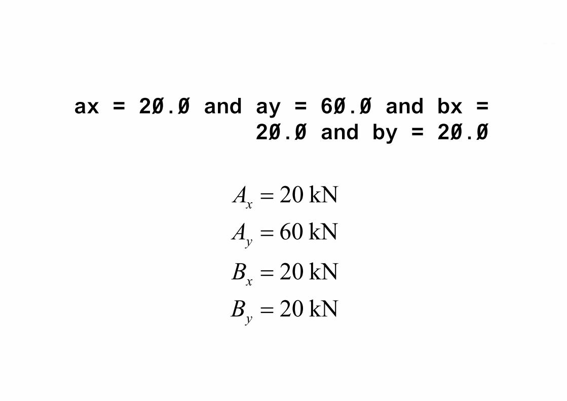
ax = 20.0 and ay = 60.0 and bx = 20.0 and by = 20.0

20 kN60 kN

20 kN20 kN

x

y

x

y

AA

BB

==

==

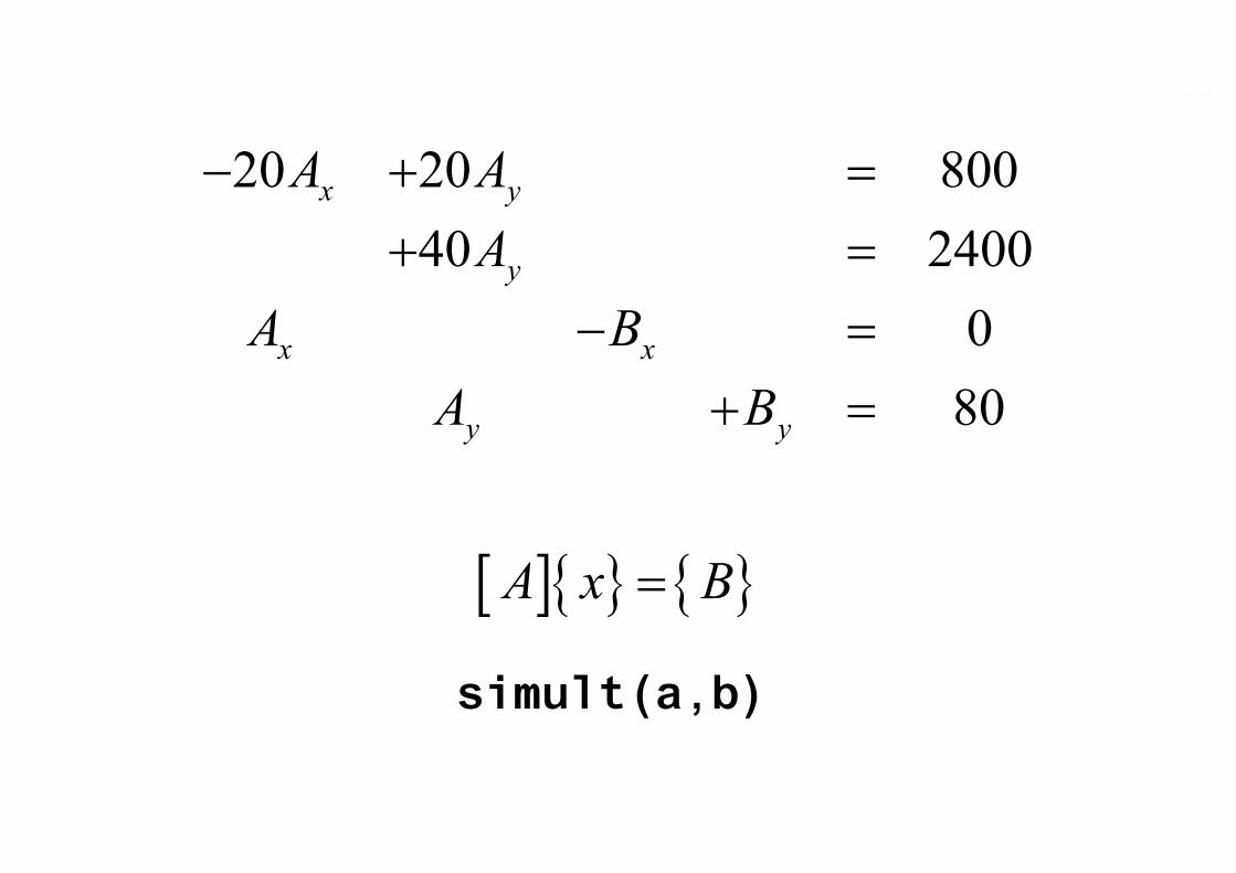
20 20 80040 2400

080

x y

y

x x

y y

A AA

A BA B

− + =+ =

− =+ =

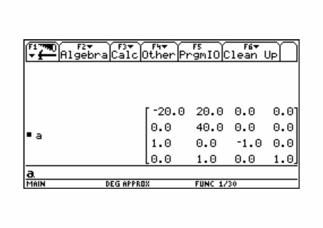
[ ]{ } { }A x B=

simult(a,b)

[ ]

20 20 0 00 40 0 01 0 1 00 1 0 1

A

− = −

{ }

8002400

080

B

=

Structural AnalysisTI voyage 200

Parabolic Cables (Samikian, example 4.4)

– System of non linear simultaneous equations

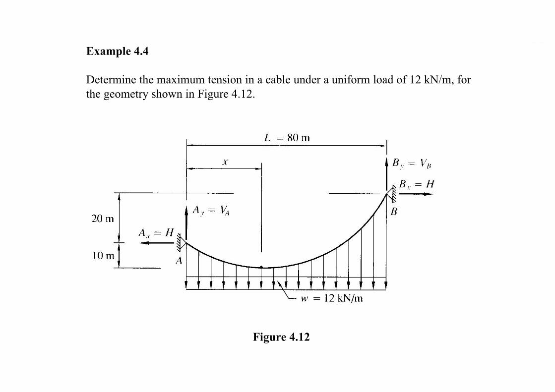
Example 4.4

Determine the maximum tension in a cable under a uniform load of 12 kN/m, for the geometry shown in Figure 4.12.

Figure 4.12

Figure 4.13

From Equation 2.8, we have for the left-hand part

2

10 02A

wxM H= − + =∑For the right-hand part, we have

2( )30 02B

w L xM H −= − =∑

From Equation 2.7, we have for the left-hand part

0y AF V wx= − =∑For the right-hand part, we have

( ) 0y BF V w L x= − − =∑

(1)

(2)

(3)

(4)

solve(-10h+w*x^2/2=0 and30h-w*(1-x)^2/2=0 and va-w*x=0 andvb-w*(l-x)=0,{x,h,va,vb})|w=12 and l=80

x = 29.3 and h = 514.5 and va = 351.4 and vb = 608.6orx = -109.3 and h = 7165.5 and va = -1311.4 and vb = 2271.4

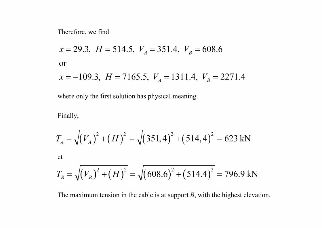
Therefore, we find

29.3, 514.5, 351.4, 608.6or

109.3, 7165.5, 1311.4, 2271.4

A B

A B

x H V V

x H V V

= = = =

= − = = =

where only the first solution has physical meaning.

Finally,

( ) ( ) ( ) ( )2 2 2 2351,4 514,4 623 kNA AT V H= + = + =

et

( ) ( ) ( ) ( )2 2 2 2608.6 514.4 796.9 kNB BT V H= + = + =

The maximum tension in the cable is at support B, with the highest elevation.

Structural AnalysisTI voyage 200

• Method of Virtual Work (Samikian, chapter 9)

– Symbolic calculations, Mohr’s integrals

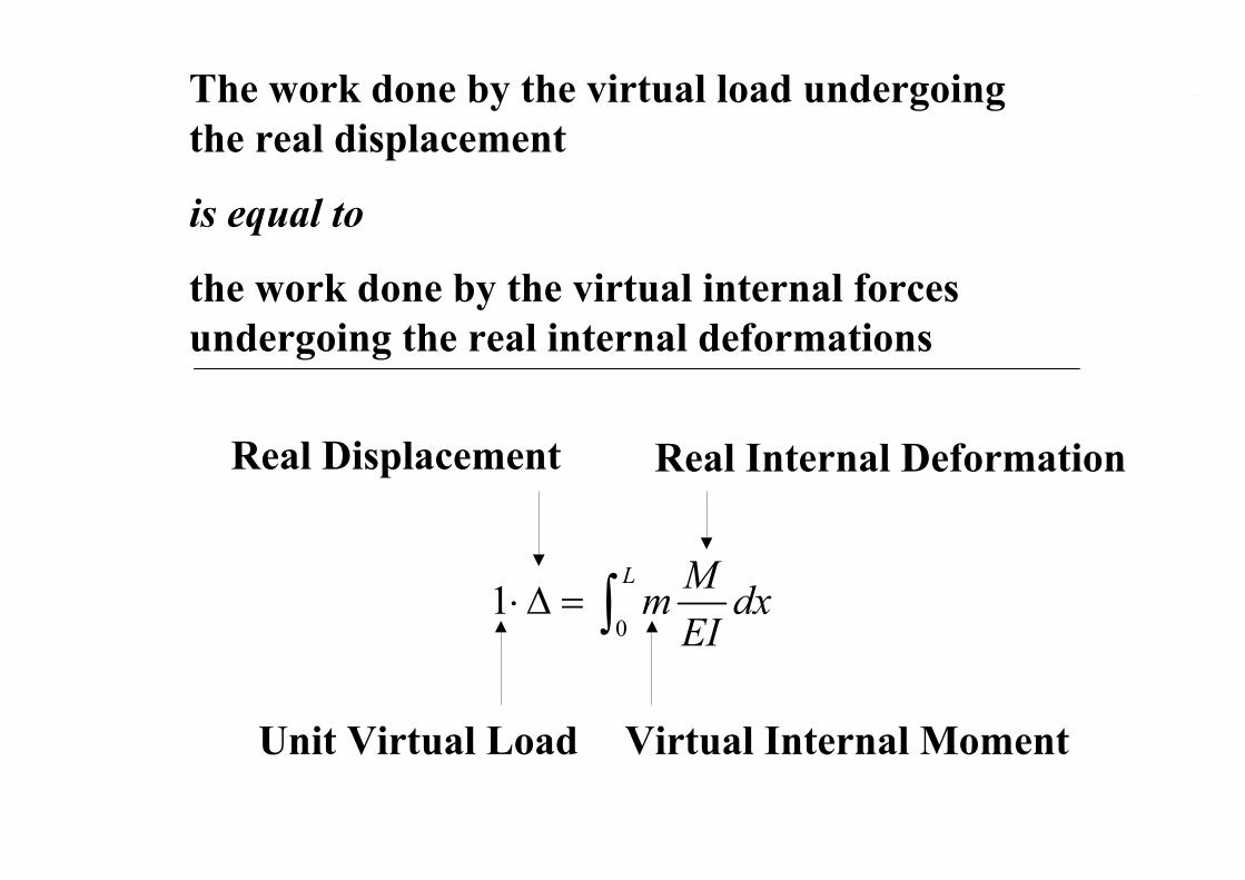
The work done by the virtual load undergoing the real displacement

is equal to

the work done by the virtual internal forces undergoing the real internal deformations

01

L Mm dxEI

⋅∆ = ∫

Real Displacement Real Internal Deformation

Unit Virtual Load Virtual Internal Moment

Example

Find the deflection at point C

La b

A C B

L

A B

w : real load

2AwLR =

2BwLR =

V

2wL

M2

max 8wLM =

2

2 2wLx wxM = −

2wL

−

SFD

BMD

FBD x

x

A B

1 : unit virtual load

AbRL

= BaRL

=

m

maxabmL

=

( )am L xL

= −

La b

bxmL

=

BMD

FBD x

x

( )

2

2 2

, 0

,

wLx wxM

bxm x aLam L x a x LL

= −

= ≤ ≤

= − ≤ ≤

01

L

CMm dxEI

⋅∆ = ∫

( )

2

0

2

( )2 2

2 2

a

C

L

a

L a x wLx wx dxL

a wLx wxL x dxL

−∆ = − +

− −

∫

∫

( )

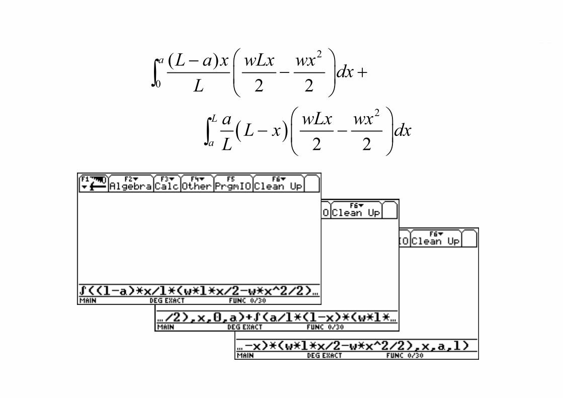
2

0

2

( )2 2

2 2

a

L

a

L a x wLx wx dxL

a wLx wxL x dxL

−− +

− −

∫

∫

2La =When

Mohr’s Integrals

Reference : « Techniques de l’ingénieur », Construction Series, Volume C5, Chapter C2555

0

1 Mmdx∫

Structural AnalysisTI voyage 200

• Coordinate Transformations

x2

y2

θ

x1

y1

F

P1

V1

– P1 sin θ

P1 cos θ

V1 cos θ

V1 sin θ

P1 cos θ + V1 sin θ

– P1 sin θ + V1 cos θ

Coordinate Transformations

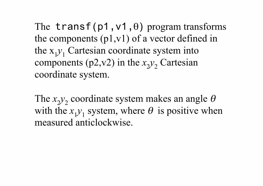
The transf(p1,v1,θ) program transforms the components (p1,v1) of a vector defined in the x1y1 Cartesian coordinate system into components (p2,v2) in the x2y2 Cartesian coordinate system.

The x2y2 coordinate system makes an angle θwith the x1y1 system, where θ is positive when measured anticlockwise.

1.Download the transf program(file : transf.9xp) from the Web site onto your computer

2.Transfer the transf program from your computer to the calculator usingTI Connect (USB cable) or TI-Graph Link (serial cable)

3.Once the program is loaded in the calculator, give the command transf(p1,v1,θ). In the following example, p1=10, v1=10*2=20 and θ = 30°.

The program displays the values of p1, v1, θ and p2, v2. Also, a drawing is shown for checking purposes.

(p1,v1,θ)Prgm

√(p1^2+v1^2)→f

tan(v1/p1)→α

p1*cos(θ)+v1*sin(θ)→p2

⁻p1*sin(θ)+v1*cos(θ)→v2

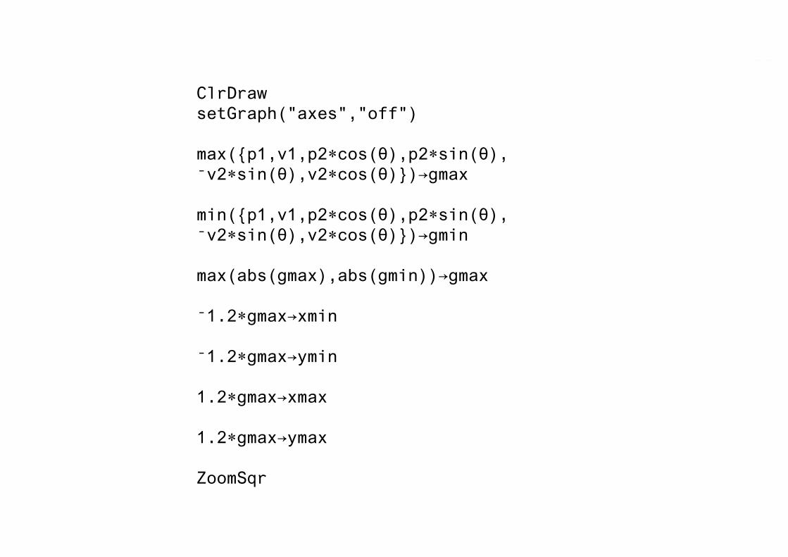
ClrDrawsetGraph("axes","off")

max({p1,v1,p2*cos(θ),p2*sin(θ),⁻v2*sin(θ),v2*cos(θ)})→gmax

min({p1,v1,p2*cos(θ),p2*sin(θ),⁻v2*sin(θ),v2*cos(θ)})→gmin

max(abs(gmax),abs(gmin))→gmax

⁻1.2*gmax→xmin

⁻1.2*gmax→ymin

1.2*gmax→xmax

1.2*gmax→ymax

ZoomSqr

PxlText "p1="&string(p1),5,0PxlText "v1="&string(v1),15,0PxlText " f="&string(f),25,0PxlText " α="&string(α),35,0

PxlText "θ="&string(θ),50,0PxlText "p2="&string(p2),60,0PxlText "v2="&string(v2),70,0

PxlText "(c)2003",83,0PxlText "D.Bauer",93,0

Line 0,0,p1,v1Line 0,0,p1,0Line 0,0,0,v1

PtText string(p1),p1,0PtText string(v1),0,v1

Pause

Line 0,0,p2*cos(θ),p2*sin(θ)Line 0,0,⁻v2*sin(θ),v2*cos(θ)

PtText string(p2),p2*cos(θ),p2*sin(θ)PtText string(v2),⁻v2*sin(θ),v2*cos(θ)

Pause

setGraph("axes","on")DispHomeEndPrgm

Structural AnalysisTI voyage 200

• Acknowledgments– The present research was made possible by

grants from the École de technologie supérieure (PSIRE-ENS 2001,2003).