Embed Size (px)
Citation preview

Using VIX Futures as Option Market-Makers’ Short Hedge
Yueh-Neng Lin∗∗∗∗
National Chung Hsing University e-mail: [email protected]
tel:+(886) 4 2285-7043; fax:+(886) 4 2285-6015
Anchor Y. Lin
National Chung Hsing University e-mail: [email protected]
tel:+(886) 4 2285-5410; fax:+(886) 4 2285-6015
Abstract
The introduction of VIX futures has been a major financial innovation that will
facilitate to a great extent the hedging of volatility risk. Using spot VIX, VIX futures,
S&P 500 futures, S&P 500 options and S&P 500 futures options, this study examines
alternate models within a delta-vega neutral strategy. VIX futures are found to
outperform vanilla options in hedging a short position on S&P 500 futures call options.
In particular, while incorporating stochastic volatility on average outperforms in
out-of-sample hedging, adding price jumps further enhances the hedging performance
for short-term options during the post-crash-relaxation period.
Keywords: VIX futures; S&P 500 futures options; Forward-start strangle; Stochastic
volatility; Price jumps
Classification code: G12, G13, G14
∗ Corresponding author: Yueh-Neng Lin, Department of Finance, National Chung Hsing University, 250, Kuo-Kuang Road, Taichung, Taiwan, Phone: (886) 4 2285-7043, Fax: (886) 4 2285-6015, Email: [email protected]. The authors thank Don M Chance and Jeremy Goh for valuable comments and suggestions that have helped to improve the exposition of this article in significant ways. The authors also thank Sol Kim, Shun Kobayashi and conference participants of the 2008 Asia-Pacific Association of Derivatives held in Busan, Korea, the 2008 Asian FA-NFA 2008 International Conference in Yokohama, Japan, the 2008 FMA Conference in Dallas, U.S.A., and the 2009 Australasian Finance and Banking Conference in Sydney, Australia for their insightful comments. Yueh-Neng Lin gratefully acknowledges research support from Taiwan National Science Council.

2
1. Introduction
The U.S. stock market crashed on October 19, 1987, when the Dow Jones
Industrials Average lost 22.6% of its market value and the S&P 500 dropped 20.4% in
one day. The 1987 crash brought volatility products to the attention of academics and
practitioners. As the booming-crash cycle of financial markets becomes often and
makes markets highly uncertain, effectively hedging volatility risk has become urgent
for market participants. Volatility and variance swaps have been popular in the OTC
equity derivatives market for about a decade. The Chicago Board Options Exchange
(CBOE) successively launched the Volatility Index (VIX) futures on March 26, 2004,
the three-month S&P 500 variance futures on May 18, 2004, the twelve-month S&P
500 variance futures on March 23, 2006, and the VIX option on February 24, 2006.
These were the first of an entire family of volatility products to be traded on exchanges.
While implied volatility can also be traded with straddles or by unwinding
delta-hedged option positions, VIX futures and options offer a cleaner and less costly
exposure which does not need to be adjusted when the market moves. Another
attractive feature is that VIX is relatively simple to track and that it can be forecasted
from several readily observable variables: the current deviation of VIX from its mean,
past realized volatility, the performance of the S&P 500, and even the month of the

3
year.1 Moran and Dash (2007) and Szado (2009) discuss the benefits of a long
exposure to VIX futures and VIX call options. Grant et al. (2007) suggest that VIX
calls have the potential to provide particularly effective diversification of equity risk,
exhibiting far higher payouts per dollar than S&P 500 puts.
VIX futures and options are important for practices since VIX is implied
volatility of the S&P 500 Index (SPX), the most widely followed index of large-cap
U.S. stocks and considered as an indicator for the U.S. economy. Many mutual funds,
index funds2 and exchange-traded funds (ETF) attempt to replicate the performance of
the SPX by holding the same stocks in the same proportions as the index. In recent
years, ETFs and index funds have become the most popular investment products
worldwide and the need for hedging price risk and volatility risk of the index-related
investment vehicles has become urgent, particularly during periods of extreme market
movements.3 The user base for using volatility instruments as extreme downside
1 The VIX uses all out-of-the-money calls and puts written on SPX with valid quotes. At-the-money call
and put options on SPX are also included with their prices averaged. It attempts to gauge the expected
risk-neutral realized return volatility over next 30 days. The VIX relies on the concept of static
replication, and thus it is not subjected to a specific option pricing model. In theory, the VIX can be used
as the fair value for the 30-day volatility forward. The VIX calculation isolates expected volatility from
other factors that could affect option prices such as dividends, interest rates, changes in the underlying
price and time to expiration. 2 Popular index funds such as SPDRs, iShares, and the Vanguard 500 are an efficient proxy for the underlying index of the S&P 500. 3 Recently, the U.S. markets have experienced highly up and down. For example, the SPX reached an all-time high of 1,565.15 on October 9, 2007 during the housing bubble and then lost approximately 57% of its value in one and one-half years between late 2008 and early 2009 surrounding the global financial crisis, reaching a nearly 13-year closing low at 676.53 on March 9, 2009. On September 15, 2008, the failure of the large financial institution Lehman Brothers, rapidly devolved into a global crisis

4
hedges and/or spread arbitrages continues to expand from sophisticated trading firms
and hedge funds to insurance companies, risk managers and fundamental investors. As
shown in Figure 1, the explosive growth of the trading volume and open interests of
futures and options on VIX in recent years clearly reflects a demand for a tradable
vehicle which can be used to hedge or to implement a view on volatility.
[Figure 1 about here]
There is also a hedge need for financial intermediaries such as option
market-makers and hedge funds who provide liquidity to end-users by taking the other
side of the end-user net demand. In reality, however, even market-makers cannot hedge
options perfectly because of the impossibility of trading continuously, stochastic
volatility, jumps in the underlying and transaction costs (Gârleanu, Pedersen and
Poteshman, 2009). In light of these facts, this study considers how options are hedged
using VIX futures by competitive risk-averse market-makers who face stochastic
volatility and jumps. The risks of an option writer can be partitioned into price risk and
volatility risk. Carr and Madan (1998) suggest options on a straddle and Brenner et al.
(2006) construct a straddle to hedge volatility risk. Those straddle positions look for a
resulting in a number of bank failures and sharp reductions in the value of equities and commodities and quickly spread into a global economic shock and recession. Stock market crashes often follow speculative market bubbles of a prolonged period of rising stock prices and excessive economic optimism and then are driven by panic as much as by underlying economic factors.

5
large price move in the underlying and thus both delta and vega risk must be
simultaneously hedged. A slightly dissenting focus is Rebonato (1999), who constructs
a forward-start strangle, consisting of two wide strangles with different maturities, so
that the changes of underlying stock price will not affect the payoff of the portfolio.
This forward-start strangle hedges forward volatility risk without exposure to delta
and gamma risk. Other than using vanilla options, Neuberger (1994) adopts the log
contract to hedge volatility. Finally, in their simulation study, Psychoyios and
Skiadopoulos (2006) hedge the instantaneous volatility using either a volatility call
option or a traditional option. They conclude that a vanilla option is a more efficient
instrument to hedge the volatility risk arisen from a short position on a European call
option than a volatility option.
The introduction of VIX futures and options has been a major financial
innovation that facilitates to a great extent the hedging of volatility risk. Since VIX
futures and options settle to the implied volatility of the S&P 500, they are effective to
cross-hedge the vega risk of stock options and stock indexes correlated to the S&P 500,
whether these are exchange-traded or embedded in other assets. The hedging
effectiveness of the new VIX derivatives is an important issue that has not yet been
concluded in the literature. This paper addresses this issue by building a delta-vega

6
neutral strategy from market-makers’ perspective and demonstrates to what extent the
risk factors such as stochastic volatility and price jumps in the S&P 500 price
dynamics influence hedging effectiveness of using VIX futures as upside hedges of a
short position on a futures call option. A short position on the SPX futures call option
is chosen as our target asset because its vega risk consists of (i) spot volatility
randomness over the period from current time and the option maturity, and (ii) forward
volatility changes between the option maturity and the underlying futures expiry. The
current price of VIX futures reflects the market’s expectation of the VIX level at
expiration, and thus VIX futures, at least in theory, should provide an effective hedge
on vega risk of SPX futures options. In particular, price fluctuations in VIX futures,
SPX futures, SPX options and SPX futures options arise endogenously through S&P
500 stocks’ response to the macroeconomic conditions. Consistent modeling of SPX,
SPX derivatives, VIX and VIX derivatives helps address the “hedging effectiveness of
VIX futures” in a unified framework. Our model generates interesting dynamics for
S&P 500, including stochastic volatility and price jumps. It also provides a novel
procedure to estimate state-dependent hedge ratios. For the purpose of comparison, a
forward-start strangle portfolio, rather than a forward-start straddle, is constructed to

7
hedge the forward volatility risk arisen from a short position on a futures call option.4
Recent empirical work on index options identifies factors such as stochastic
volatility, jumps in prices and jumps in volatility. The results in the literature regarding
these issues are mixed. For example, tests using option data disagree over the
importance of price jumps: Bakshi et al. (1997) find substantial benefits from including
jumps in prices, whereas Bates (2000) and others find that such benefits are
economically small, if not negligible. Pan (2002) finds that pricing errors decrease
when price jumps are added for certain strike-maturity combinations, but increase for
others. Eraker (2004) finds that adding jumps in returns and volatility decreases errors
by only 1%. Bates (2000) finds a 10% decrease, but it falls to around 2% when
time-series consistency is imposed. Broadie et al. (2007) find strong evidence for
jumps in prices and modest evidence for jumps in volatility for the cross section of
SPX futures option prices from 1987 to 2003. Furthermore, while studies using the
time series of returns unanimously support jumps in prices, they disagree with respect
to the importance of jumps in volatility. To learn about rare jumps and stochastic
4 On the one hand, since the present value profile of straddle as a function of spot around the at-the-money level is less flat than strangle, the delta and gamma of a straddle are less close to zero than a strangle. On the other hand, VIX futures offer a way for investors to buy and sell option volatility without having to explicitly deal with factors that have an impact on the value of the SPX option position such as delta and gamma. This study thus uses a forward-start strangle, instead of a forward-start straddle, as a benchmark to hedge the forward volatility risk arisen from a short position on a futures call option.

8
volatility, and investors’ attitudes toward the risks these factors embody, Figure 2
displays a time-series plot of the VIX against the SPX over January 1990 to June 2009.
In empirical index option hedging, Bakshi et al. (1997) find that once the stochastic
volatility is modeled, the hedging performance may be improved by incorporating
neither price jumps, nor stochastic interest rates into the SPX option pricing framework.
Bakshi and Kapadia (2003) use Heston’s (1993) stochastic-volatility option pricing
model to construct a delta-hedged strategy for a long position on SPX call options.
They find that the volatility risk is priced and the price jump affects the hedging
efficiency. Vishnevskaya (2004) follows the structure of Bakshi and Kapadia (2003)
and constructs a delta-vega-hedged portfolio consisting of the underlying stock,
another option and the money-market fund, for a long position on the SPX call option.
His result suggests the existence of some other sources of risk.
Guided by previous studies, this study considers both stochastic volatility and
price jumps, denoted the “SVJ” model. 5 The setup contains the competing
stochastic-volatility (SV) futures option formula as special cases. Since SPX futures
option contracts are American-style, it is important to take into account the extra value
5 Our results could be generalized by introducing a time-varying jump intensity, jumps in the volatility, or a more complicated correlation structure for the state variables. While such generalization would add realism, this study wants to test the effect of the VIX futures in the presence of the most basic sources of incomplete market risk considered here.

9
accruing from the ability to exercise the options prior to maturity. One can follow such
a nonparametric approach as in Aït-Sahalia and Lo (1998) and Broadie et al. (2000) to
price American options. Closed-form option pricing formulas, however, make it
possible to derive hedge ratios analytically. Therefore, for options with early exercise
potential, this paper computes a quadratic approximation for evaluating American
futures options. The approximation is based on the one developed by MacMillan
(1987), examined by Barone-Adesi and Whaley (1987) for the constant-volatility
process, extended by Bates (1991) for the jump-diffusion process, and modified by
Bates (1996) for the SV and SVJ processes. For the SV and SVJ processes, this
approximation is consistent with Bates (1996) for evaluating American currency
futures options.
In sum, this study examines using VIX futures as vega hedges required for a
short position on the SPX futures call option, and compares its effectiveness against
traditional “synthetic long volatility” hedging instruments such as forward-start
strangle. The study also considers how options are priced by competitive risk-averse
market-makers who cannot hedge perfectly due to stochastic volatility and price jumps
in the underlying SPX. Our findings reveal that VIX futures generally outperform
forward-start strangle over the out-of-sample hedging period, August 2006−June 2009.

10
These diagnostics document the extraordinary significance in our hedging exercise that
occurred following the stock market crash on September 15, 2008. Based on empirical
analyses, this paper concludes that using VIX futures as vega hedges of a short position
on a SPX futures call option on average provides superior hedging effectiveness than a
forward-start strange portfolio. In addition, adding price jumps into the SPX price
process further improve hedging performance for short-term cases during the
post-crash-relaxation period.
The rest of this paper proceeds as follows. Next section illustrates hedging
strategies. Pricing models for calculating delta and vega hedge ratios are presented in
Section 3. Section 4 summarizes data and model parameter estimation procedure.
Section 5 presents summary statistics of parameter estimates and in-sample pricing
errors. Section 6 analyzes out-of-sample hedging results. Section 7 finally concludes.
2. Hedging Strategies
A time-t short position on the 1T -matured call option written on 2T -matured
SPX futures is used as the target portfolio, i.e. )(FCTARA
tt −= for 21 TTt << . This
study then constructs two hedging schemes to hedge the target position.

11
Hedging Scheme 1 (HS1): The instrument portfolio consists of tN ,1 shares of
underlying SPX futures, and tN ,2 shares of forward-start strangle portfolios. One unit
of forward-start strangle portfolio consists of a short position on a 1T -matured
strangle and a long position on a 2T -matured strangle, given by
),,(),,(),,(),,( 12221121 KTSpKTScKTSpKTScINSTE
t
E
t
E
t
E
tt ++−−= (1)
where ),,( 21 KTScE
t and ),,( 22 KTSc
E
t are 2K -strike SPX call options with
maturities 1T and 2T , respectively. ),,( 11 KTSpE
t and ),,( 12 KTSpE
t are 1K -strike
SPX put options with maturities 1T and 2T , respectively.
Hedging Scheme 2 (HS2): The instrument portfolio consists of tN ,1 shares of
underlying SPX futures, and tN ,2 shares of the VIX futures, i.e.,
)(F 1
VIXTINST tt = (2)
where )(F 1
VIXTt is the time-t price of the VIX futures with expiry 1T .
The gain or loss of this hedged portfolio is expressed by
)()( ,22,1 FCINSTNTFNA
tttttt −+=π (3)
Further add the constraints of delta-neutral and vega-neutral by
0)(
,2,1 =∂
∂−
∂
∂+=
∂
∂
t
A
t
t
ttt
t
t
F
FC
F
INSTNN
F
π (4)

12
0)(
,2 =∂
∂−
∂
∂=
∂
∂
t
A
t
t
tt
t
t FCINSTN
ννν
π (5)
The shares of instrument assets are computed as
t
tt
t
A
tt
F
INSTN
F
FCN
∂
∂−
∂
∂= ,2,1
)( (6)
∂
∂
∂
∂=
t
t
t
A
tt
INSTFCN
νν/
)(,2 (7)
The illustrations of t
A
t FFC ∂∂ /)( , tt FINST ∂∂ / , t
A
t FC ν∂∂ /)( and ttINST ν∂∂ / for
alternate models are provided in the following section.
Next, this study couples these two hedging schemes with the SV and the SVJ
option models to construct four hedging strategies: HS1-SV, HS1-SVJ, HS2-SV and
HS2-SVJ. Assuming that there are no arbitrage opportunities, the hedged portfolio tπ
should earn the risk-free interest rate r. In other words, the change in the value of this
hedged portfolio over t∆ is expressed as
)1( −=−=∆ ∆∆+∆+
tr
tttttt eππππ (8)
where )]()([][)]()([ ,222,1 FCFCINSTINSTNTFTFNA
t
A
tttttttttttt −−−+−=∆ ∆+∆+∆+∆+π .
The hedging error as a function of rebalancing frequency Δ� is defined as the
additional profit (loss) over the risk-free return and it can be written as
)]()()[1(
)]()([][)]()([
)1()(
,22,1
,222,1
FCINSTNTFNe
FCFCINSTINSTNTFTFN
ettHE
A
ttttt
tr
A
t
A
tttttttttt
tr
tttt
−+−−
−−−+−=
−−∆=∆+
∆
∆+∆+∆+
∆∆+ ππ
(9)

13
Finally, compute the average absolute hedging error:
���Δ�� � �1/�∑ |�� ������� �� � �Δ����� �����|���� (10)
, and the average dollar-value hedging error:
�������Δ�� � �1/�∑ �� ������� �� � �Δ����� ��������� (11)
where � ��� � ��/� and 1T is the expiry of the target SPX futures call option.
Measurements of hedging performances are based on the framework proposed in
previous papers, for instance, Bakshi et al. (1997) and Psychoyios and Skiadopoulos
(2006).
3. Empirical Pricing Models
Hedging strategies are constructed using SPX futures, SPX options, SPX futures
options, VIX futures and VIX. Therefore, their fair value and related greeks are
required for further empirical analyses. The most general process considered in this
paper is the jump-diffusion and stochastic volatility (SVJ) process of Bates (1996) and
Bakshi et al. (1997). This general process contains stochastic volatility (SV) of Heston
(1993) as a special case.
3.1 The SVJ Process for SPX Prices
14
Contingent claims are priced as if investors were risk-neutral and under the SVJ
model the SPX price follows the jump-diffusion with stochastic volatility
ttttStttJJt dNSJdSSbdS ++−= , )( ωνµλ (12)
where b is the cost of carry coefficient (0 for futures options and δ−r for stock
options with a cash dividend yield δ ). tJ is the percentage jump size with mean Jµ .
The jumps in the asset log-price are assumed to be normally distributed, i.e.,
),(~)1ln( 2
JJt NJ σθ+ . Satisfying the no-arbitrage condition, 1)2/exp( 2 −+= JJJ σθµ .
tN is the jump frequency following a Poisson process with mean Jλ . The
instantaneous variance tν of the index follows a risk-neutral mean-reverting square
root process
tttt ddtd , )( νννν ωνσνκθν +−= (13)
where νκ is the speed of mean-reverting adjustment of tν ; /ν νθ κ is the long-run
mean of tν ; νσ is the variation coefficient of tν ; and tS ,ω and t,νω are two
correlated Brownian motions with the correlation coefficient ),( ,, ttS ddcorrdt νωωρ = .
3.2 Fair Value to SPX Options
SPX options are European-style. Bakshi et al. (1997) provide the time-t value of
SPX call and put options with strike K and maturity T for the SVJ model:

15
2
)(
1
)(),,( Π−Π= −−−− tTrtT
t
E
t KeeSKTSc δ (14)
)1()1(),,( 2
)(
1
)( −Π−−Π= −−−− tTrtT
t
E
t KeeSKTSpδ (15)
where 1Π and 2Π are risk-neutral probabilities that are recovered from inverting the
characteristic functions 1f and 2f , respectively,
∫∞
−
−+=−Π
0
ln );,,;,(Re
1
2
1),,;,( ϕ
ϕ
ϕν
πν
ϕ
di
rStTtferSKtT
ttj
Ki
ttj (16)
for j = 1, 2. The characteristic functions 1f and 2f for the SVJ model are given in
equations (A12) and (A13) of Bakshi et al. (1997). Delta and vega of the European
SPX options are given in equation (13) of Bakshi et al. (1997). Finally, delta and vega
of the forward-start strangle portfolio can be calculated straightforward.
3.3 Fair Value to SPX Futures Options
Since SPX futures options are American-style, it is important, in principle, to
take into account the extra value accruing from the ability to exercise the options prior
to maturity. Referred to Bates (1996), the futures call option is
≥−
<
+
≡
*
22
*
2*
221
1
/)( if )(
/)( if /)(
),,(),,(
2
ctt
ct
q
c
tE
tA
t
yKTFKTF
yKTFy
KTFKAKTFC
KTFC (17)
where ])([),,( 212
)(
11 Π′−Π′= −−
KTFeKTFC t
tTrE
t is the time-t price of a European-style

16
futures call option with strike K and expiry 1T . )( 2TFt is the time-t futures price
with maturity 2T . For j=1, 2, jΠ′ are the relevant tail probabilities for evaluating
futures call options, which are the same to jΠ in equation (16) except replacing K
with )( )( 12 TTrKe
−−− δ . ]/)1,,(1)[/( 1
*
2
*
2 tc
E
tc FTyCqyA ∂∂−= . For the SVJ process, 2q is
the positive root to the equation of q given as follows
0]1)1[(12
1
2
1 2/)1(
)(
2 2
1=−++
−−
−−+ −
−−Jqqq
JJtTrJJ ee
rqq
σµλνµλν (18)
ν is the expected average variance over the lifetime of the option conditional on no
jumps, i.e., )(
]1[
1
)( 1
tT
etT
t−
−
−+=
−−
ν
κ
ν
ν
ν
ν
κκ
θν
κ
θν
ν
. The critical futures price/strike price
ratio 1* ≥cy above which the futures call is exercised immediately is given implicitly
by
∂
∂−
+=−
t
c
E
tcc
E
tcF
TyC
q
yTyCy
)1,,(1 )1,,(1 1
*
2
*
1
** (19)
The closed form solutions to the parameters 2q and *
cy are provided for given model
parameters and for given maturity 1T . Since linear homogeneity in underlying asset
and strike holds for European options, by Euler theorem the following equations
sustain:
)(),,(1
)1,,( 21
)(
111 Π′−Π′== −−
c
tTrE
tc
E
t yeKTFCK
TyC (20)
1
)(11 11),,(1)1,,(
Π′=∂
∂=
∂
∂ −− tTr
t
E
t
t
c
E
t eKF
KTFC
KF
TyC (21)

17
where KTFy tc /)( 2= . Replacing )1,,( 1TyC c
E
t and t
c
E
t
F
TyC
∂
∂ )1,,( 1 of *
cy in equation
(19) with equations (20) and (21), the solution to *
cy is given by
1
)(
22
2
)(*
1
1
111
1
1
Π′
−+−
Π′−=
−−
−−
tTr
tTr
c
eKqq
ey (22)
Thus, the solution to 2A is computed as
Π′−
Π′
−+−
Π′−= −−
−−
−−
1
)(
1
)(
22
2
)(
21
1
1 11
11
]1[ tTr
tTr
tTr
eK
eqK
q
eA (23)
Finally, the calculation for delta and vega of the futures call option is straightforward.
3.4 Fair Value to VIX Futures
From Lin (2007), the time-t fair price of the VIX futures expiring at 1T under
the SVJ model is given by
2/3
0
2
2
0
0
21
VIX
)(1
8
)(
)(1
)(F
01010
11
0
01010
+++
+
−+++≡
−−
−−
−−
τττ
τ
τττ
βνατ
ζ
ντ
βνατ
ζ
baa
DCa
baaT
tTttT
tTttT
tTttTt
(24)
where 365/300 =τ , )(22 JJJ θµλζ −= , )( 1
1
tT
tT e−−
− = νκα , )1( 11 tTtT −− −= α
κ
θβ
ν
ν ,
ν
τκ
τκ
ν )1( 0
0
−−=
ea , )(
00 0 τ
ν
ντ τ
κ
θab −= , )( 2
2
111 tTtTtTC −−− −= αακ
σ
ν
ν , 2
2
2
)1(2
11 tTtTD −− −= α
κ
θσ
ν
νν ,
0
0)VIX( 2
2
0
τ
τζτν
a
bt
t
−−≡ .

18
Pricing formulas and related greeks for the SV model are obtained as a special
case of the general model with price jumps restricted to zero, i.e., 0=ttdNJ and thus
Jλ =Jµ =
Jσ =0.
4. Data and Estimation Procedure
The sample period spans from July 3, 2006, through June 30, 2009. Spot VIX,
spot SPX, daily midpoints of the last bid and last ask quotations for SPX options, and
daily settlement prices for VIX futures are obtained from the CBOE. Daily settlement
prices for SPX futures and daily settlement SPX futures options are obtained from
CME. The averages of U.S. Treasury bill bid and ask discounts, collected from
Datastream, with maturity closest to an option’s maturity are used as risk-free interest
rates. Because SPX option contracts are European-style, index levels are adjusted for
dividends by the subtraction of the present value of future cash dividend payments
(from S&P Corporation) before each option’s expiration date.
The contracts that are selected for empirical analyses are described as follows:
First, the selected SPX futures contracts expire in March, June, September and
December. Second, the SPX futures call options that expire in February, May, August
and November are selected as the target portfolio. Third, the forward-start strangle

19
portfolio involves in two strangles. This study uses the SPX options contracts that
expire in February, May, August and November to construct a short-term strangle, and
that expire in March, June, September, and December for another long-term strangle.
Finally, the VIX futures that expire in February, May, August and November are
selected as the hedging instrument.
Several exclusion filters are applied to construct the option price data. First, as
options with less than six days to expiration may induce liquidity-related biases, they
are excluded from the sample. Second, to mitigate the impact of price discreteness on
option valuation, option prices lower than 3/8 are excluded. Finally, option prices that
violate the upper and lower boundaries are not included in the sample. Based on these
criteria, 29.90% and 10.50% of the original selected SPX options and SPX futures call
options are eliminated, respectively. A total of 24,761 records of joint SPX futures call
options (20,839 records), SPX options (3,200 observations), and VIX futures (722
records) are used for parameter estimation.
Table 1 reports descriptive properties of the SPX futures call options, SPX
futures, VIX futures and VIX for each moneyness-maturity category where moneyness
is defined as the SPX futures price divided by the SPX futures call option’s strike price,
i.e., KTFt /)( 2 . Out of 20,839 SPX futures call option observations, about 50% is

20
out-of-the-money (OTM) and 35% is at-the-money (ATM). By maturity, 6,221
transactions are under 30 days to maturity, 8,613 are between 30 and 60 days to
maturity, and 6,005 are more than 60 days to maturity. The average futures call price
ranges from 5.57 points for short-term (<30 days) deep out-of-the-money (DOTM) call
options to 118.56 points for medium-term (30-60 days) deep in-the-money (DITM)
call options. Its underlying SPX futures price ranges from 947.85 points for short-term
DOTM calls to 1,347.89 points for medium-term ATM calls.
The average VIX futures prices range from 21.02 corresponding to the
medium-term ATM calls to 46.23 for the short-term DOTM calls. The VIX varies from
20.68 (for medium-term ATM call options) to 50.87 (for short-term DOTM call
options). The price of a VIX futures contract to VIX is an analogy to what a 30-day
forward interest rate is to a 30-day spot interest rate. The price of a VIX futures
contract can be lower, equal to or higher than VIX, depending on whether the market
expects volatility to be lower, equal to or higher in the 30-day forward period (covered
by the VIX futures) than in the 30-day spot period (covered by VIX). Owing to the
tendency of VIX to have a negative correlation with the SPX, the VIX futures prices
have traded at a discount to the VIX before contract settlement especially during the
in-crash period, September 15, 2008 to December 31, 2008.

21
A total of 800 records of simultaneous strikes 1K and 2K of SPX options are
used for the construction of the forward-start strangle over the sample period,
consisting of 722 trading days. Average option quotes of 1K range from 599.89 for
DOTM short-term futures calls to 1,100.31 for ATM short-term futures calls, whereas
average option quotes of 2K range 1,066.82 for short-term DOTM futures calls to
1,464.49 for medium-term ATM futures calls.
[Table 1 about here]
This study uses SPX options to construct the forward-start strangle that expire in
the February Quarterly Cycle as 1T -strangle and that expire in the March Quarterly
Cycle as 2T -strangle. Therefore, the pair of ( 1T , 2T ) data must be February−March,
May−June, August−September and November−December. The strike 1K ( 2K ) is the
minimum (maximum) strike of the SPX put (call) option, which expire in the February
and March Quarterly Cycles simultaneously. To enhance the integrity of the study, less
heavily traded SPX options are eliminated here. On the basis of an analysis of patterns
of trading volumes on SPX options, four pairs of maturity-strike combinations are
selected from the option contracts retained to form a forward-start strangle on each
trading day: ),( 11 KT and ),( 12 KT of SPX puts, and ),( 21 KT and ),( 22 KT of SPX
calls. There are in total 3,200 SPX option observations, consisting of 1,600 SPX calls

22
and 1,600 SPX puts. Those option observations compose of 800 pairs of calls with
strike 2K and puts with strike 1K . The selected strikes 1K of the SPX puts are on
average 938.03 index points, whereas the strikes 2K of the SPX calls are on average
1,377.21. Table 2 reports the average point of those SPX option and the observation for
each moneyness-maturity category over the period, 3 July 2006 to 30 June 2009.
Moneyness is defined as the current SPX value divided by the SPX option’s strike, S/K.
The average call prices range from 1.3716 points for short-term OTM call options to
59.4300 points for long-term near-the-money call options. The average put prices
range from 0.4125 points for short-term OTM put options to 66.8500 points for
long-term near-the-money put options.
[Table 2 about here]
The vector of structural parameters Φ for alternate processes is backed out by
minimizing the sum of the squared pricing errors between option and futures model
and market prices over the period, July 3, 2006 to May 14, 2009 (the last trading day of
May-matured SPX futures call options in 2009). The minimization is given by
∑∑= =
ΦΦ−
T tN
t
N
n
nn CC1 1
2* )]([min (25)
where TN is the number of trading days in the estimation sample, tN is the number
of SPX futures call options, SPX options and VIX futures on day t, and nC and *
nC

23
are the observed and model option or futures prices, respectively. The parameters of
the SV and the SVJ models are estimated separately each month and thus Φ are
assumed to be constant over a month. The assumption that the structural parameters are
constant over a month is justified by an appeal to parameter stability (Bates, 1996;
Eraker, 2004; Zhang and Zhu, 2006). The estimation period is chosen because the
settlement day of the SPX futures option is the third Friday of contract months. Hence,
the month is defined as the period from the third Friday of the prior calendar month to
the third Thursday of this calendar month. Table 3 reports the monthly average of each
estimated parameter series and the monthly averaged in-sample mean squared errors
for the SV and SVJ models, respectively.
[Table 3 about here]
Since SPX futures options are American, we follow Broadie et al.’s (2007)
procedure to account for the early exercise feature. Our calibration procedure begins
by converting American market prices to equivalent European market prices, and
estimates model parameters based on European prices. This allows us to use
computationally efficient European pricing routines that render the large-scale
calibration procedure feasible. Using the observed price � we compute an American
binomial-tree implied volatility, that is, a value ��� such that � � �!���� , �,

24
where �! denotes the binomial-tree American option price. We then estimate that an
equivalent European option would trade in the market at a price $���� , �, where
$ denotes the Black (1976) European option price.
5. Risk-Neutral Parameter Estimates and In-Sample Pricing Fit
Summary statistics for instantaneous volatility and risk-neutral parameter
estimates from the SV and SVJ models implicit in SPX futures calls prices, VIX
futures prices and SPX option prices along with in-sample mean squared errors are
shown in Table 3. In 2008, a series of bank and insurance company failures triggered a
financial crisis that effectively halted global credit markets and required unprecedented
government intervention.6 These failures caused a crisis of confidence that made
banks reluctant to lend money amongst themselves, or for that matter, to anyone. The
time-series plot of the VIX against the SPX in Figure 2 sheds light on these issues.
Other than the entire sample period, we divide our data into four sub-periods: (i) the
period prior to the Lehman Brothers bankruptcy: July 3, 2006 to August 14, 2008, and
(ii) the 2008 crash fear periods: August 15, 2008 to December 18, 2008; August 15,
6 In 2008, Fannie Mae (FNM) and Freddie Mac (FRE) were both taken over by the government.
Lehman Brothers declared bankruptcy on September 14th after failing to find a buyer. Bank of America
agreed to purchase Merrill Lynch, and American International Group was saved by an $85 billion capital
injection by the government. Shortly after, on September 25th, J P Morgan Chase agreed to purchase the
assets of Washington Mutual in what was the biggest bank failure in history. In fact, by September 17,
2008, more public corporations had filed for bankruptcy in the U.S. than in all of 2007.

25
2008 to June 18, 2009; and December 19, 2008 to June 18, 2009.7
Model-specific estimates of implicit distributions indicate extremely turbulent
conditions in the joint markets of SPX futures, SPX futures options, SPX options and
VIX futures over September 2008-December 2008, with somewhat quieter conditions
over January 2009-June 2009 following the end of the Lehman Brothers bankruptcy.
Indeed, Table 3 finds parameter estimates of the SV and SVJ models from their full
July 2006�June 2009 sample diverge from estimates for a September 2008�June 2009
subsample. The estimates of jump-frequency intensity %& that capture outliers indicate
the major shocks that affected the markets over September 2008�December 2008. The
possibility of SPX price jumps occurs with an average size '& of �0.13, �0.12, and
�0.11 (with jump size uncertainty �&( estimated at 0.35, 0.30, and 0.49) for the July
2006�August 2008, September 2008�December 2008, and January 2009�June 2009
periods, respectively.
The risk-neutral mean-reverting volatility process is controlled by three
parameters: the long-term mean, )'*/+*, to which variance reverts, the speed of
reversion, +*, and the variation coefficient, �*. For instance, on the basis of mean
7 The data split, for example, August 14, 2008 and December 18, 2008, is chosen because the estimation
month is defined as the period from the third Friday of the prior calendar month to the third Thursday of
this calendar month.

26
values of ,+* , )'*/+*, �*- � .5.77,0.3458,0.776 for the SV model and
.3.93,0.5862,1.806 for the SVJ model over the crash period, volatility took 30 and 44
trading days to revert halfway toward a long-term mean of 34.58% for the SV model
and 58.62% for the SVJ model, respectively.8 The mean speed of reversion value of
5.77 and 3.19 for the SV model over the crash periods (Panels C and D) is higher than
the values of 0.86 (Panel B) and 1.47 (Panel E) over the pre- and post-crash-relaxation
periods. However, it is close to the value of 5.02 found by the SVJ model over the
post-crash-relaxation period. The average long-term mean variance '*/+* of 34.36%
for the SVJ model over the crash period compares with values of 3.91% in the
pre-crash period and 13.33% in the post-crash-relaxation period. The variation
coefficient, �*, determines how fat-tailed the distribution is and thereby the relative
values of deep OTM options versus near-the-money options. The mean value of 1.80
found in the SVJ model over the crash period compares with values of 0.22 and 0.46
over the pre- and post-crash-relaxation periods. The consistently negative estimates of
: indicate that implied volatility and index returns are negatively correlated. This
means the implied distribution perceived by SPX option traders, SPX futures option
traders and VIX futures traders is negatively skewed. The mean values of : for the
8 The half-life of volatility shocks for the square-root process was calculated as
;<�(�
=>? 252 trading
days.

27
SVJ model reached �0.91 in the crash period and �0.97 in the post-crash-relaxation
period. An explanation for these extreme values is that a relatively continuous bear
market in the SPX starting from September 15, 2008 caused investors to perceive the
underlying distribution as being heavily left skewed. The SV model captures this effect
by attaching a higher value to :. The mean value of : of �0.57 for the SV model in
the pre-crash period compares with more extreme values of �0.75 in the crash period
and �0.77 in the post-crash-relaxation period. The implied volatilities, )@ % ,
estimated by alternate models are able to capture the substantial 2008 crash. In
particular, the SVJ model adds a price-jump component that directly captures the 2008
outliers. Table 3 also gives the � values for the parameter estimates of the index price
process. These results indicate that all parameter estimates are significantly different
from zero at the 90% confidence interval.
The parameter estimates in Table 3 are interesting in light of estimates obtained
in prior studies. Bakshi et al. (1997) estimate the jump frequency for the SVJ model as
a 0.59 annualized jump probability, and the jump-size parameter B& and �& are
�5.37% and �7%, respectively. Their estimate of +* and �* are 2.03 and 0.38. Pan
(2002), Bates (2000) and Eraker (2004) assume that the jump frequency depends on
the spot volatility. The average jump intensity point estimates in Pan (2002) are in the

28
range [0.07, �0.3%] across different model specifications, whereas Eraker (2004)
indicates two to three jumps in a stretch of 1,000 trading days. Interestingly, Bates
(2000) obtains quite different results, with an average jump intensity of 0.005. Bates
(2000) also reports a jump size mean ranging from �5.4% to �9.5% and standard
deviations of about 10% to 11%. Hence, Bates’ estimates imply more frequent and
more severe crashes than the parameter estimates reported in Bakshi et al. (1997) and
Eraker (2004). Our estimates are in the same ballpark as those reported in Bates
(1996).
Finally, the fact that allowing pricing jumps to occur enhances the SV model’ fit
is illustrated by the model’s average of the squared pricing errors between the market
price and the model price in an average month (C�). The in-sample mean squared
errors are considerably and consistently smaller for more complicated models.
However, the resulting increase in C� for the various specifications is significant
under the crash period, suggesting that this jump risk assessment fails to capture the
substantial 2008 crash.9
9 Bates (2006) found the stochastic-intensity jump model fits S&P returns better than the
constant-intensity specification, when jumps are drawn from a finite-activity normal distribution or
mixture of normals.

29
6. Hedging Results
The need for a perfect delta-neutral hedge can arise in situations where not only
is the underlying price risk present, but also are volatility and jump risks in our
specifications. In conducting this exercise, however, we should first recognize that a
perfect hedge may not be practically feasible in the presence of stochastic jump sizes
(for example, for the SVJ model). The difficulty is seen from the existing work by
Bakshi et al. (1997), Bates (1996), Cox and Ross (1976), and Merton (1976). For this
reason, whenever jump risk is present, we follow Merton (1976) and only aim for a
partial hedge in which diffusion risks are completely neutralized but jump risk is left
uncontrolled for. We do this with the understanding that the overall impact on hedging
effectiveness of not controlling for jump risk can be small or large, depending on
whether the hedge is frequently rebalanced or not.
To examine the hedging effectiveness, at time � short the SPX futures call
option and establish the hedge using two hedging schemes under three SPX price
processes. The hedger will need a position in some D�, shares of the underlying SPX
futures (to control for price risk), and some D(, units of either forward-start strangles
or VIX futures to control for volatility risk @ . The study uses the previous month’s
structural parameters and the current day’s (t) SPX, SPX futures, SPX futures options,

30
SPX options, VIX futures and U.S. Treasury-bill rates to construct the hedged portfolio.
Next, this study calculates the hedging error as of day � � 1 if the hedge is rebalanced
daily or as of day � � 5 if the rebalancing takes place every five days. These steps are
repeated for each futures call option that expires in February quarterly cycle and every
trading day in the sample. Finally, the average absolute and the average dollar hedging
errors for each moneyness-maturity category are then reported for each model in
Tables 4 and 5.
In Table 4, under the SV model, the hedging errors of HS1 are from 1.09 points
(DOTM short-term of five-day revision in the pre-crash period) to 33.97 points (ATM
short-term of five-day revision in the crash period), whereas the hedging errors of HS2
range from 0.98 points (DOTM middle-term of one-day revision in the pre-crash
period) to 38.86 points (ATM short-term of five-day revision in the crash period). For
the SVJ model, HS1 has hedging errors from 1.13 points (DOTM middle-term of
one-day revision in the pre-crash period) to 216.96 points (ITM middle-term of
one-day revision in the post-crash-relaxation period), whereas HS2 has hedging errors
from 1.15 points (DOTM short-term of one-day revision in the pre-crash period) to
33.46 points (DITM short-term of five-day revision in the crash period).
When the hedge revision frequency changes from daily to once every five days,

31
the hedging errors increase, except for the HS1-SVJ short-term options in the
post-crash-relaxation period. Though HS1 outperforms HS2 in some cases within
short-term categories under five-day rebalancing, the HS1 performs poorly in daily
rebalancing coupled with SVJ; for example, its absolute hedging errors are 141.85 for
futures options with ATM1 and short-term, 216.96 with ITM and middle-term, and
140.00 with DITM and short-term during the post-crash-relaxation period (Panel E).
The findings shed a light on instability issues of HS1’s hedging performance.
Improvement by the stochastic-volatility models (SV and SVJ) is more evidence
when the HS2 strategy is adopted, which indicates a consequence of better model
specifications. A striking pattern emerging from this table is that, with respect to
short-term options in the post-crash-relaxation period (Panel E) and short-term ITM
and DITM options during the two in-crash periods (Panels C and D), the SVJ model
coupled with HS2 has virtually smaller hedging errors. It represents the random price
jump feature commonly exists in the SPX price process, especially in the in-crash
periods. Noticeably, for the options in the other remaining moneyness-maturity
categories, however, adding price jumps to the SV model does not improve its hedging
performance. Thus, except for short-term DITM options, the result in the pre-crash
period (Panel B), however, seems to be consistent with those of Bakshi et al. (1997)

32
and Bakshi and Kapadia (2003), which show the hedging superiority of the SV model
relative to the SVJ model. Note that the parameter of jump-frequency intensity Jλ in
Bakshi et al. (1997) is 0.59, i.e. one year and half for a price jump to occur, which is
comparable to 0.60 of our empirical work only in the pre-crash period. Based on daily
or every five-day rebalancing, Bakshi et al. (1997) conclude that the reason for the SV
model dominates the SVJ model in terms of hedging performance is the chance for a
price jump to occur is small in the daily or five-day rebalancing period. The estimated
parameter Jλ in the crash (post-crash-relaxation) period, however, is 9.97 (1.02)
larger than that of Bakshi et al. (1997). For this reason, whenever jump risk is present,
the overall impact on short-term hedging effectiveness of not allowing for jump risk is
significant. Therefore, Bakshi et al.’s (1997) reason does not completely hold for our
empirical results. Another possible reason is that the SPX futures options used in this
study are American-style, while SPX options are European-style for prior research.
Since the traders with American-style options positions have early-exercise choice and
thus can take caution to prevent any loss from the potential jump events than the ones
with European-style options. Thus, American-style option buyers (sellers) may even
favor (hate) volatility risk than the ones with European-style options. In addition, given
the possibility of price jumps, the specification of SVJ can provide more accurate

33
parameter estimates than SV (Bates, 1996). Thus, the delta-vega-neutral strategy could
be constructed in a more effective way under SVJ than SV. It is thus not surprising for
our hedging results for some short-term options showing that the SVJ model
outperforms the SV model in the crash-related periods.
Further, the HS1 hedge of the SVJ model results in poor hedging errors
comparable to that of the SV model during the post-crash-relaxation period, which
suggests that model misspecification may have a significant effect on hedging when
using the HS1 strategy through the crash periods. Instead, adopting HS2 hedge strategy
has more robust hedging performance in magnitude across the SV and SVJ models.
Out of 60 moneyness–maturity combinations within 1-day revision frequency reported
in Table 4, absolute hedging error was lower for the HS2 strategy in 58 cases than the
HS1 strategy. The improvement was generally indistinguishable between the
crash-related periods and the pre-crash period. About the maturity impact on hedging
performance, there is no pattern showing the difference between hedging schemes
decreases with maturity and increases with maturity, as discovered by Psychoyios and
Skiadopoulos (2006) for ITM and OTM target options. In terms of the moneyness
effect, our results show that the absolute hedging errors of HS1 and HS2 strategies
have the tendency to increase with moneyness. In contrast, Psychoyios and

34
Skiadopoulos (2006) find that the options perform best for ATM and worse for ITM,
and the difference between hedging schemes is minimized for ATM and maximized for
ITM. In sum, the results indicate that the forward-start strangle portfolio is in general a
less efficient instrument to hedge forward volatility risk than VIX futures.
[Table 4 about here]
Theoretically, if a portfolio is perfectly hedged, it should earn the risk-free rate
of interest, and the average hedging errors should be close to zero. In this study, the
hedging error is defined as the changes in the value of the hedged portfolio minus the
risk-free return. Table 5 reports the average hedging errors. If the figure is greater (less)
than zero, it means that the strategy gets more (less) profits than risk-free return.
During the in-crash period, the dollar hedging errors are relatively sensitive to
revision frequency. Another pattern to note from Table 5 is that the HS1 and HS2’s
1-day revision dollar hedging errors are always positive for short-term options in the
post-crash-relaxation period, indicating that both HS1 and HS2 underhedge each target
option, whereas the dollar hedging errors of the other periods are more random and can
take either sign. Therefore, the HS1 and HS2 strategies exhibit a systematic hedging
bias during the post-crash-relaxation period, while they do not in the other periods. Out
of 60 moneyness–maturity combinations within 1-day revision frequency reported in

35
Table 5, dollar hedging errors were lower for the HS2 strategy in 49 cases than for the
HS1 strategy, indicating VIX futures that are volatility sensitive as a superior hedge
instrument.
[Table 5 about here]
7. Conclusion
This study has extended a parsimonious American futures option pricing model
that admits stochastic volatility and random price jumps. It is shown that this
closed-form pricing formula is practically implementable, leads to useful analytical
hedge ratios, and contains the stochastic-volatility option formula as a special case.
This last feature has made it relatively straightforward to study the relative empirical
hedging performance of the three models. In particular, the study considers whether
and by how much VIX futures improve option hedging by competitive risk-averse
dealers or investors who have a short position on SPX futures call options. For the
purpose of comparison, a forward-start strangle portfolio is constructed for managing
forward volatility.
This study then couples two hedging schemes (HS1 and HS2) with two SPX
price processes (SV and SVJ) to hedge the target asset. On the one hand, SPX futures
and the forward-start strangle portfolio are used to construct two hedging strategies

36
(HS1−SV and HS1−SVJ). On the other hand, SPX futures and VIX futures are used to
construct the other two hedging strategies (HS2−SV and HS2−SVJ).
There are some interesting empirical findings. First, HS2 in general dominates
HS1, suggesting that the VIX futures contract is a more efficient instrument to hedge
forward volatility risk than a forward-start strangle portfolio. This finding contributes
to the existing literature documented by Psychoyios and Skiadopoulos (2006), who
point out that volatility options are less powerful instruments to hedge a short position
on a European call option than plain-vanilla options, and that the most naïve volatility
option-pricing model can be reliably used for pricing and hedging purposes. Second,
gauged by the absolute hedging errors, while the SVJ model performs slightly better
for short-term options during the post-crash-relaxation period, the SV model coupled
with HS2 achieves better performance for the remaining cases. This finding is slightly
different from that obtained by Bakshi et al. (1997). Overall, our results support the
claim that the VIX futures contract is a better alternative to the traditional
forward-start strangle, if the target is a futures call option, or equivalently if the risk
exposures to forward volatility randomness. This is because the VIX futures contract
not only performs much better in a stochastic-volatility and/or price-jump economy but
also is practically implementable.

37
The contributions of this paper are threefold. First, closed-form solutions to
American futures options under three SPX price processes are derived. Second, the
concept of forward volatility risk applied to VIX futures and a forward-start strangle
portfolio is introduced. Third, this study derives the hedging weights of VIX futures
and the forward-start strangle portfolio that will be convenient to practical participants
for risk management purposes.

38
References
Aït-Sahalia, Y., Lo, A. W., 1998. Nonparametric estimation of state-price densities
implicit in financial asset prices. Journal of Finance 53, 499−548.
Bakshi, G., Cao, C., Chen, Z., 1997. Empirical performance of alternative option
pricing models. Journal of Finance 52, 5, 2003−2049.
Bakshi, G., Kapadia, N., 2003. Delta-hedged gains and the Negative market volatility
risk premium. Review of Financial Studies 16, 527−566.
Barone-Adesi, G., Whaley, R., 1987. Efficient analytic approximation of American
option values. Journal of Finance 42, 301−320.
Bates, D.S., 1991. The crash of ’87: Was it expected? The evidence from options
markets. Journal of Finance 46, 1009−1044.
Bates, D.S., 1996. Jumps and stochastic volatility: exchange rate processes implicit in
Deutsche Mark options. Review of Financial Studies 9, 69−107.
Bates, D.S., 2000. Post-’87 crash fears in the S&P 500 futures option market. Journal
of Econometrics 94, 181−238.
Bates, D.S., 2006. Maximum likelihood estimation of latent affine processes. Review
of Financial Studies 19, 909−965.
Black, F., 1976. The pricing of commodity contracts. Journal of Financial Economics 3,

39
167−179.
Brenner, M., Galai, D., 1989. New financial instruments for hedging changes in
volatility. Financial Analysts Journal 45, 61−65.
Brenner, M., Ou, E. Y., Zhang, J. E., 2006. Hedging volatility risk. Journal of Banking
and Finance 30, 811−821.
Broadie, M., Chernov, M., Johannes, M., 2007. Model specification and risk premia:
Evidence from futures options. Journal of Finance 62, 1453−1490.
Broadie, M., Detemple, J., Ghysels, E., Torrés, O., 2000. American options with
stochastic dividends and volatility: A nonparametric investigation. Journal of
Econometrics 94, 53−92.
Carr, P., Madan, D., 1998. Towards a theory of volatility trading, Chapter in Volatility,
in: Jarrow, R. (Ed.), Volatility, Risk Publications, pp. 417−427.
Chaput, J. S., Ederington, L. H., 2005. Volatility trade design. Journal of Futures
Markets 25, 243−279.
Cox, J., Ross, S., 1976. The valuation of options for alternative stochastic processes.
Journal of Financial Economics 3, 145−166.
Eraker, B., 2004. Do equity prices and volatility jump? Reconciling evidence from spot
and option prices. Journal of Finance 59, 1367−1403.

40
Gârleanu, N., Pedersen, L. H., Poteshman, A. M., 2009. Demand-based option pricing.
Review of Financial Studies 22, 4259−4299.
Grant, M., Gregory, K., Lui, J., 2007. Considering all options. Working paper,
Goldman Sachs Global Investment Research.
Heston, S., 1993. A closed-form solution for options with stochastic volatility with
applications to bond and currency options. Review of Financial Studies 6, 2,
327−343.
Lin, Y. N., 2007. Pricing VIX futures: Evidence from integrated physical and
risk-neutral probability measures. Journal of Futures Markets 27, 1175−1217.
MacMillan, L. W., 1987. Analytic approximation for the American put options.
Advances in Futures and Options Research 1A, 119−139.
Merton, R., 1976. Option pricing when the underlying stock returns are discontinuous.
Journal of Financial Economics 4, 125−144.
Moran, M. T., Dash, S., 2007. VIX futures and options: Pricing and using volatility
products to manage downside risk and improve efficiency in equity portfolios.
Journal of Trading 2, 96−105.
Neuberger, A., 1994. The log contract. Journal of portfolio management 20, 2, 74−80.
Pan, J., 2002. The jump-risk premia implicit in options: Evidence from an integrated

41
time-series study. Journal of Financial Economics 63, 3−50.
Psychoyios, D., Skiadopoulos, G., 2006. Volatility options: Hedging effectiveness,
pricing, and model error. Journal of Futures Markets 26, 1, 1−31.
Rebonato, R., 1999. Volatility and Correlation: In the Pricing of Equity, FX, and
Interest-Rate Options. John Wiley, New York.
Szado, E., 2009. VIX futures and options—A case study of portfolio diversification
during the 2008 financial crisis. Journal of Alternative Investments, forthcoming.
Vishnevskaya, A., 2004. Essays in option pricing: Vega-hedged gains and the volatility
risk premium. Working paper, University of Virginia.
Zhang, J. E., Zhu, Y., 2006. VIX futures. Journal of Futures Markets 26, 521−531.

42
Table 1 Sample Properties of S&P 500 Futures Call Options, S&P 500 Futures, VIX Futures, VIX and Selected SPX Options
The average points of futures call options ($250 per point), the average points of underlying futures ($250 per point), the average points of VIX futures ($1,000 per point), the average points of VIX, the average strikes K1 and K2 of selected SPX options and the total number of futures call options are presented in each moneyness-maturity category. Contract months of both futures call options and VIX futures are in the February Quarterly Cycle, whereas contract months of SPX futures are in the March Quarterly Cycle. K1 and K2 are selected strikes of SPX put and call options to construct forward-start strangles, both of which expire on the maturity dates of the SPX futures call and the SPX futures simultaneously. We divide the futures option data and contemporaneous futures levels, VIX futures, VIX, K1 and K2 into several categories according to either moneyness or term to expiration. Define Ft(T2)/K as the time-t intrinsic value of a futures call. A futures call is then said to be deep out-of-the-money (DOTM) if its Ft(T2)/K<0.94; out-of-the-money (OTM) if Ft(T2)/K ∈[0.94,0.97); at-the-money (ATM) if Ft(T2)/K ∈[0.97,1.03); in-the-money (ITM) if Ft(T2)/K ∈[1.03,1.06); and deep in-the-money (DITM) if Ft(T2)/K≧1.06. By the term to expiration, an option contract can be classified as (i) short-term (<30 days); (ii) medium-term (30-60 days); and (iii) long-term (>60 days). The data period is from July 3, 2006 to June 30, 2009.
Days to Maturity Moneyness <30 30−60 >60 Subtotal
DOTM <0.94
SPX futures call 5.5696 6.8933 8.4643 SPX futures 947.8534 1078.1347 1167.9128 VIX futures 46.2295 34.2556 30.4921 VIX 50.8742 38.7459 32.2216 K1 599.8907 720.3157 793.8094 K2 1066.8182 1255.1761 1340.5847 Observation 869 2,867 3,053 6,789
OTM 0.94−0.97
SPX futures call 7.7356 12.3137 17.0321 SPX futures 1231.1835 1323.0393 1328.2712 VIX futures 29.7906 23.3573 21.4009 VIX 30.5768 23.3098 20.9756 K1 972.7829 1005.5325 1002.6713 K2 1345.6457 1456.6037 1464.8980 Observation 875 1,615 1,226 3,716
ATM1 0.97−1.00
SPX futures call 13.8811 22.9812 33.3377 SPX futures 1311.4333 1345.6390 1320.7551 VIX futures 23.3768 21.3924 21.7445 VIX 23.6443 20.9470 21.1742 K1 1100.3112 1046.4877 998.3112 K2 1400.5785 1464.4924 1458.7431 Observation 1,478 1,704 903 4,085
ATM2 1.00−1.03
SPX futures call 33.7082 44.3218 55.6945 SPX futures 1306.8449 1347.8856 1305.5544 VIX futures 23.2381 21.0243 22.9012 VIX 23.3762 20.6828 22.1135 K1 1100.1285 1050.9091 974.7164 K2 1394.2252 1463.4335 1445.6805 Observation 1,323 1,331 529 3,183
ITM 1.03−1.06
SPX futures call 62.0779 72.8389 84.7926 SPX futures 1225.0017 1292.5961 1217.1777 VIX futures 28.9174 25.3501 27.0426 VIX 29.3179 25.5828 27.1678 K1 987.9844 960.6031 850.1330 K2 1328.0622 1421.9455 1364.6277 Observation 707 514 188 1,409
DITM ≧1.06
SPX futures call 109.8420 118.5584 116.0519 SPX futures 1060.5809 1070.8000 1041.5613 VIX futures 35.8835 34.9171 35.6560 VIX 36.5378 36.1897 36.7596 K1 806.5996 695.8935 634.9057 K2 1165.8359 1213.4278 1156.9811 Observation 969 582 106 1,657
Subtotal 6,221 8,613 6,005 20,839

43
Table 2 Sample Characteristics of S&P 500 Index Options Out-of-the-money and near at-the-money SPX call and put options are selected in this study to construct
forward-start strangles, both of which expire on the maturity dates of the SPX futures call and the SPX
futures simultaneously. The average points of the SPX options ($100 per point) and the total number of
the SPX options are presented in each moneyness-maturity category. Contract months of SPX options
are in the February and March quarterly Cycles. This study classifies those observations into short-term
(<30 days), medium-term (30–60 days), and long-term (>60 days). Moneyness is defined as S/K where S
is the price of the SPX and K is the strike price of SPX options. DOTM (DITM), OTM (ITM), ATM1
(ATM2), ATM2 (ATM1), ITM (OTM) and DITM (DOTM) for calls (puts) are defined by Moneyness
<0.94, 0.94–0.97, 0.97–1.00, 1.00–1.03, 1.03–1.06, and >1.06, respectively. The data period is from July
3, 2006 to June 30, 2009.
Days to Expiration
Call Put
Moneyness <30 30–60 >60 Subtotal <30 30–60 >60 Subtotal
DOTM Option price 1.5607 3.8948 8.2840 0.5031 2.1075 3.0217
Observation 105 293 812 1,210 192 452 930 1,574
OTM Option price 1.3716 6.2070 15.9739 0.4125 8.4417 53.9000
Observation 74 146 110 330 8 9 1 18
ATM1 Option price 4.9698 16.5250 59.4300 12.5417 31.3625 66.8500 Observation 24 26 10 60 3 4 1 8
ATM2 Option price NA NA NA NA NA NA
Observation 0 0 0 0 0 0 0 0
ITM Option price NA NA NA NA NA NA
Observation 0 0 0 0 0 0 0 0
DITM Option price NA NA NA NA NA NA
Observation 0 0 0 0 0 0 0 0
Subtotal 203 465 932 1,600 203 465 932 1,600

44
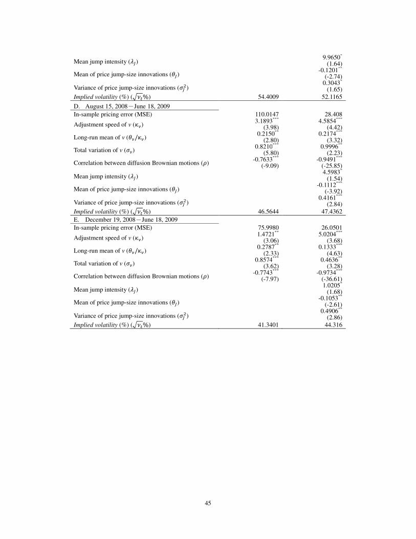
Table 3 Implied Parameter Estimation The in-sample mean squared pricing errors (C�) and estimated structural parameters reported in Panel
A are their averages over 36 nonoverlapping estimation months from the whole sample period, July 3,
2006 to June 18, 2009, with a total of 20,839 SPX futures calls, 722 VIX futures, and 3,200 SPX options.
Panel B presents estimation results that obtained preceding the Lehman Brothers bankruptcy on
September 15, 2008. Panels C, D and E report parameter estimates and in-sample mean squared errors
that occurred covering the stock market crash on September 15, 2008. We divide the post-’08 crash fears
in the S&P 500 market into three periods: August 15, 2008 to December 18, 2008, August 15, 2008 to
June 18, 2009, and December 19, 2008 to June 18, 2009. The instantaneous variance of the S&P 500
index, @ , is replaced by VIX and structural parameters, given by
00
/])VIX([2
2
0 ττζτν abtt
−−≡
where 365/300
=τ , )(22 JJJ
θµλζ −= ,ντντ κτθ /)(
00 0ab −= ,
ν
τκ
τ κν /)1( 0
0
−−= ea ,and B& � �EF�GFH/( � 1.
The figures within parentheses are the �-statistics of parameter estimates. The symbols of ***, ** and *
indicate significance of �-statistics at the 1%, 5% and 10% levels, respectively. IJ�� LM� SV SVJ
A. July 3, 2006-June 18, 2009
In-sample pricing error (C�) 67.7801 17.5971
Adjustment speed of ν (+*) 1.5071***
(4.90) 3.8388***
(8.30)
Long-run mean of ν ('*/+*) 0.1838***
(6.26) 0.0886***
(3.91)
Total variation of ν (�*) 0.7548***
(12.54) 0.4363***
(3.18)
Correlation between diffusion Brownian motions (:) -0.6254***
(-12.90) -0.7844***
(-13.22)
Mean jump intensity (%&) 1.7078**
(1.95)
Mean of price jump-size innovations ('&) -0.1248***
(-6.35)
Variance of price jump-size innovations (�&() 0.3698***
(6.51) Implied volatility (%) ()@ %) 26.1041 27.0852
B. July 3, 2006-August 14, 2008
In-sample pricing error (MSE) 51.5359 13.4391
Adjustment speed of ν (+*) 0.8602***
(4.62) 3.5516***
(7.05)
Long-run mean of ν ('*/+*) 0.1718***
(5.95) 0.0391***
(5.80)
Total variation of ν (�*) 0.7294***
(11.30) 0.2197***
(4.98)
Correlation between diffusion Brownian motions (:) -0.5723***
(-10.15) -0.7211***
(-9.26)
Mean jump intensity (%&) 0.5961**
(2.34)
Mean of price jump-size innovations ('&) -0.1301***
(-5.17)
Variance of price jump-size innovations (�&() 0.3520***
(6.20) Implied volatility (%) ()@ %) 18.2347 19.2580
C. August 15, 2008-December 18, 2008
In-sample pricing error (MSE) 161.0398 31.9449
Adjustment speed of ν (+*) 5.7651***
(7.80) 3.9328*
(2.20)
Long-run mean of ν ('*/+*) 0.1196*
(1.99) 0.3436**
(2.36)
Total variation of ν (�*) 0.7664***
(8.50) 1.8034*
(1.72)
Correlation between diffusion Brownian motions (:) -0.7467**
(-4.37) -0.9127***
(-10.46)
45
Mean jump intensity (%&) 9.9650*
(1.64)
Mean of price jump-size innovations ('&) -0.1201**
(-2.74)
Variance of price jump-size innovations (�&() 0.3043*
(1.65) Implied volatility (%) ()@ %) 54.4009 52.1165
D. August 15, 2008-June 18, 2009
In-sample pricing error (MSE) 110.0147 28.408
Adjustment speed of ν (+*) 3.1893***
(3.98) 4.5854***
(4.42)
Long-run mean of ν ('*/+*) 0.2150**
(2.80) 0.2174***
(3.32)
Total variation of ν (�*) 0.8210***
(5.80) 0.9996**
(2.23)
Correlation between diffusion Brownian motions (:) -0.7633***
(-9.09) -0.9491***
(-25.85)
Mean jump intensity (%&) 4.5983*
(1.54)
Mean of price jump-size innovations ('&) -0.1112***
(-3.92)
Variance of price jump-size innovations (�&() 0.4161***
(2.84) Implied volatility (%) ()@ %) 46.5644 47.4362
E. December 19, 2008-June 18, 2009
In-sample pricing error (MSE) 75.9980 26.0501
Adjustment speed of ν (+*) 1.4721**
(3.06) 5.0204***
(3.68)
Long-run mean of ν ('*/+*) 0.2787**
(2.33) 0.1333***
(4.63)
Total variation of ν (�*) 0.8574***
(3.62) 0.4636**
(3.28)
Correlation between diffusion Brownian motions (:) -0.7743***
(-7.97) -0.9734***
(-36.61)
Mean jump intensity (%&) 1.0205*
(1.68)
Mean of price jump-size innovations ('&) -0.1053**
(-2.61)
Variance of price jump-size innovations (�&() 0.4906**
(2.86) Implied volatility (%) ()@ %) 41.3401 44.316

46
Table 4 Absolute Hedging Errors
The figures in this table denote the average points of absolute hedging errors ($250 per point):
MetltHEM
l
lMtr
tlt/|)(|
1
)(
)1(∑ =
−∆
∆−+∆+ where � ��� � ��/∆� and �� is the maturity date of SPX
futures call options. The hedging error between time t and time t t+ ∆ is defined as )( ttHEt
∆+ . The
instrument portfolio of hedging scheme 1 (HS1) consists of t
N ,1
shares of �(-matured SPX futures,
and t
N ,2 shares of forward-start strangle portfolios. The forward-start strangle portfolio consists of a
short position on a 1
T -matured strangle and a long position on a 2
T -matured strangle. The instrument
portfolio of hedging scheme 2 (HS2) consists of t
N ,1 shares of �(-matured SPX futures, and
tN
,2
shares of the VIX futures )(F1
VIXT
t with expiry
1T . This study classifies hedging errors into
moneyness-maturity categories. Define L ��(�/O as the time-t intrinsic value of a futures call. A
futures call is then said to be deep out-of-the-money (DOTM) if its L ��(�/O<0.94; out-of-the-money
(OTM) if L ��(�/O∈[0.94,0.97); at-the-money (ATM) if L ��(�/O∈[0.97,1.03); in-the-money (ITM) if
L ��(�/O∈[1.03,1.06); and deep in-the-money (DITM) if L ��(�/O≧1.06. By the term to expiration,
an option contract can be classified as (i) short-term (<60 days); (ii) medium-term (60-180 days); and
(iii) long-term (>180 days). The out-of-sample hedging period is from 21 July 2006 to 18 June 2009.
Moneyness Hedging Scheme Model
1-Day Revision Days-to-Expiration
5-Day Revision
Days-to-Expiration <60 60�180 >180 <60 60�180 >180
A. Jul 21, 2006�Jun 18, 2009
DOTM
HS1 SV 6.3632 5.6973 NA 9.5021 10.3761 NA
SVJ 33.4637 8.1925 NA 24.1823 9.2254 NA
HS2 SV 4.8084 1.9527 NA 8.6915 3.3650 NA
SVJ 5.3711 2.2702 NA 9.2961 3.8778 NA
OTM
HS1 SV 5.1153 NA NA 9.5244 NA NA
SVJ 27.9749 NA NA 20.6359 NA NA
HS2 SV 3.8156 NA NA 9.5799 NA NA
SVJ 4.2278 NA NA 10.3038 NA NA
ATM1
HS1 SV 5.9481 7.8628 NA 11.3570 10.7725 NA
SVJ 32.5398 11.1507 NA 22.4562 14.2753 NA
HS2 SV 4.6932 4.0339 NA 11.4669 7.2320 NA
SVJ 4.9902 5.1210 NA 11.7750 9.0196 NA
ATM2
HS1 SV 8.6628 8.8071 NA 16.8057 13.1141 NA
SVJ 23.1278 12.8809 NA 23.5359 18.5878 NA
HS2 SV 7.3054 5.6731 NA 17.1326 10.9915 NA
SVJ 7.5161 7.1724 NA 17.3088 13.6157 NA
ITM
HS1 SV 9.2380 10.8061 5.2657 18.7035 17.9655 6.7988
SVJ 25.5432 60.2912 7.9828 23.0510 43.0296 9.6633
HS2 SV 8.9247 7.3065 2.3606 21.5786 14.4162 3.9708
SVJ 8.7227 9.7977 3.2370 20.9328 19.1125 5.3365
DITM
HS1 SV 12.5563 10.4566 NA 27.3971 17.2110 NA
SVJ 77.5575 20.3055 NA 49.8613 31.2482 NA
HS2 SV 13.8977 8.5752 NA 31.0028 14.4759 NA

47
SVJ 12.4760 14.2575 NA 28.8017 25.3368 NA
B. Jul 21, 2006�Aug 14, 2008
DOTM
HS1 SV 1.6271 1.2178 NA 1.0857 1.6810 NA
SVJ 1.2366 1.1325 NA 1.1520 1.4655 NA
HS2 SV 1.1006 0.9832 NA 1.9167 1.6103 NA
SVJ 1.1500 1.3442 NA 1.2992 2.1122 NA
OTM
HS1 SV 1.9532 NA NA 2.2629 NA NA
SVJ 2.0454 NA NA 2.8458 NA NA
HS2 SV 1.2986 NA NA 2.2892 NA NA
SVJ 1.4350 NA NA 2.3661 NA NA
ATM1
HS1 SV 3.9689 5.9950 NA 5.8632 8.1794 NA
SVJ 4.2744 5.4708 NA 6.5958 7.9208 NA
HS2 SV 3.0985 3.0499 NA 5.6791 6.2113 NA
SVJ 3.3586 3.6063 NA 5.6930 7.4192 NA
ATM2
HS1 SV 6.7815 6.5657 NA 10.5221 10.2949 NA
SVJ 7.1242 6.7447 NA 11.2855 10.8328 NA
HS2 SV 5.4907 4.5320 NA 10.2085 9.8554 NA
SVJ 5.9103 5.3767 NA 10.1996 11.5051 NA
ITM
HS1 SV 6.7833 6.4763 3.2729 12.7463 14.1034 3.8647
SVJ 6.8680 6.8006 2.2594 12.3273 14.4697 3.1666
HS2 SV 6.5618 6.2657 1.4700 14.5355 15.4006 2.6745
SVJ 7.3731 7.3726 1.8959 13.6645 18.2209 3.5430
DITM
HS1 SV 12.3294 8.0027 NA 13.0597 13.3174 NA
SVJ 11.7860 9.5670 NA 12.5780 13.6326 NA
HS2 SV 13.8723 7.9045 NA 17.2277 15.7472 NA
SVJ 12.3444 10.9772 NA 13.5022 19.9988 NA
C. Aug 15, 2008�Dec 18, 2008
DOTM
HS1 SV 10.2786 10.7445 NA 15.5854 21.1990 NA
SVJ 11.2412 3.4474 NA 16.7245 5.2536 NA
HS2 SV 8.6603 3.1539 NA 15.0282 4.7203 NA
SVJ 10.0824 3.0954 NA 16.2191 4.6470 NA
OTM
HS1 SV 11.3648 NA NA 22.1098 NA NA
SVJ 12.4328 NA NA 23.6604 NA NA
HS2 SV 8.1884 NA NA 22.8581 NA NA
SVJ 9.5830 NA NA 23.8533 NA NA
ATM1
HS1 SV 12.3432 13.8284 NA 26.0009 18.7455 NA
SVJ 13.6087 12.3066 NA 27.1859 13.8196 NA
HS2 SV 9.1173 9.2577 NA 27.9439 11.4061 NA
SVJ 9.9005 10.6086 NA 28.5429 12.5987 NA
ATM2
HS1 SV 15.3990 14.9844 NA 33.9719 20.0752 NA
SVJ 16.1772 15.0249 NA 35.2682 18.5841 NA
HS2 SV 13.4468 11.2431 NA 38.8582 14.7783 NA
SVJ 13.7320 12.6910 NA 18.3527 17.0005 NA
ITM
HS1 SV 13.2632 18.0270 10.4035 25.5016 25.9797 14.3131
SVJ 13.9370 16.7372 8.8769 24.8437 22.4414 10.4882
HS2 SV 12.4548 12.6016 6.6167 31.9561 17.6768 8.8610
SVJ 11.1111 13.7276 7.5838 30.7140 20.0581 9.6245
DITM
HS1 SV 14.1390 11.6558 NA 27.9134 17.7928 NA
SVJ 14.2067 23.5612 NA 26.3868 29.3993 NA
HS2 SV 17.1347 10.9146 NA 35.8170 14.5072 NA
SVJ 15.3151 17.4858 NA 33.4585 27.7136 NA
D. Aug 15, 2008�Jun 18, 2009
DOTM HS1 SV 6.8930 9.0560 NA 10.4435 16.8957 NA

48
SVJ 37.0684 13.4860 NA 26.7583 15.0437 NA
HS2 SV 5.2231 2.6797 NA 9.4492 4.6807 NA
SVJ 5.8432 2.9646 NA 10.1906 5.2016 NA
OTM
HS1 SV 8.2775 NA NA 16.7859 NA NA
SVJ 53.9044 NA NA 38.4259 NA NA
HS2 SV 6.3326 NA NA 16.8706 NA NA
SVJ 7.0206 NA NA 18.2415 NA NA
ATM1
HS1 SV 9.2950 12.8060 NA 20.6474 17.6350 NA
SVJ 80.3381 26.1824 NA 49.2772 31.0923 NA
HS2 SV 7.3899 6.6382 NA 21.2546 9.9331 NA
SVJ 7.7493 9.1297 NA 22.0601 13.2551 NA
ATM2
HS1 SV 11.6729 13.8663 NA 26.8594 19.4776 NA
SVJ 48.7336 26.7312 NA 43.1366 36.0919 NA
HS2 SV 10.2091 8.2489 NA 28.2111 13.5557 NA
SVJ 10.0855 11.2256 NA 28.6836 18.3797 NA
ITM
HS1 SV 10.9667 15.2887 10.6587 22.8986 21.9639 14.7396
SVJ 38.6948 115.6698 23.4721 30.6029 72.5975 27.2455
HS2 SV 10.5887 8.3841 4.7710 26.5385 13.3971 7.4790
SVJ 9.6730 12.3084 6.8665 26.0513 20.0356 10.1905
DITM
HS1 SV 12.5792 11.0456 NA 28.8393 18.1454 NA
SVJ 84.1736 22.8828 NA 53.6117 35.4760 NA
HS2 SV 13.9003 8.7362 NA 32.3885 14.1708 NA
SVJ 12.4892 15.0447 NA 30.3407 26.6179 NA
E. Dec 19, 2008�Jun 18, 2009
DOTM
HS1 SV 3.7577 6.4093 NA 5.6818 10.1500 NA
SVJ 60.9855 29.2222 NA 36.0501 30.3903 NA
HS2 SV 2.0401 1.9362 NA 4.2829 4.6185 NA
SVJ 1.9175 2.7597 NA 4.6079 6.0710 NA
OTM
HS1 SV 5.0210 NA NA 11.1703 NA NA
SVJ 97.6484 NA NA 54.0004 NA NA
HS2 SV 4.3751 NA NA 10.5551 NA NA
SVJ 4.3178 NA NA 12.3222 NA NA
ATM1
HS1 SV 6.4850 11.3596 NA 15.7121 16.0640 NA
SVJ 141.8543 45.8117 NA 69.6426 55.5268 NA
HS2 SV 5.7975 2.9326 NA 15.0879 7.8492 NA
SVJ 5.7661 7.0376 NA 16.0837 14.1836 NA
ATM2
HS1 SV 8.0172 12.2382 NA 19.8811 18.6074 NA
SVJ 80.6758 43.7772 NA 50.8566 61.5858 NA
HS2 SV 7.0324 3.8890 NA 17.7650 11.7753 NA
SVJ 6.5077 9.0916 NA 18.0233 20.3881 NA
ITM
HS1 SV 8.7341 12.4852 11.0451 20.3680 17.8525 15.3854
SVJ 62.7648 216.9580 45.5696 36.2021 123.9478 52.6163
HS2 SV 8.7745 4.0662 1.9765 21.2714 9.0154 5.3865
SVJ 8.2749 10.8555 5.7805 21.5181 20.0125 11.0474
DITM
HS1 SV 11.3346 10.0777 NA 29.5781 18.7047 NA
SVJ 139.9982 21.8067 NA 75.3337 45.1149 NA
HS2 SV 11.3197 5.2808 NA 29.6530 13.6371 NA
SVJ 10.2345 11.1726 NA 27.8531 24.8800 NA

49
Table 5 Average Hedging Errors
The figures in this table denote the average points of hedging errors ($250 per point):
MetltHEM
l
lMtr
tlt/)(
1
)(
)1(∑ =
−∆
∆−+∆+ where � ��� � ��/∆� and �� is the maturity date of SPX futures
options. The hedging error between time t and time t t+ ∆ is defined as )( ttHEt
∆+ . The instrument
portfolio of hedging scheme 1 (HS1) consists of t
N ,1
shares of �(-matured SPX futures, and t
N ,2
shares of forward-start strangle portfolios. The forward-start strangle portfolio consists of a short
position on a 1
T -matured strangle and a long position on a 2
T -matured strangle. The instrument
portfolio of hedging scheme 2 (HS2) consists of t
N ,1 shares of �(-matured SPX futures, and
tN
,2
shares of the VIX futures )(F1
VIXT
t with expiry
1T . This study classifies hedging errors into
moneyness-maturity categories. Define L ��(�/O as the time-t intrinsic value of a futures call. A
futures call is then said to be deep out-of-the-money (DOTM) if its L ��(�/O<0.94; out-of-the-money
(OTM) if L ��(�/O∈[0.94,0.97); at-the-money (ATM) if L ��(�/O∈[0.97,1.03); in-the-money (ITM) if
L ��(�/O∈[1.03,1.06); and deep in-the-money (DITM) if L ��(�/O≧1.06. By the term to expiration,
an option contract can be classified as (i) short-term (<60 days); (ii) medium-term (60-180 days); and
(iii) long-term (>180 days). The out-of-sample hedging period is from 21 July 2006 to 18 June 2009.
Moneyness
Hedging
Scheme Model
1-Day Revision Days-to-Expiration 5-Day Revision
Days-to-Expiration
<60 60�180 >180 <60 60�180 >180 A. Jul 21, 2006�Jun 18, 2009
DOTM
HS1 SV 2.6751 1.7914 NA 5.8495 0.4414 NA
SVJ 27.0928 -0.7557 NA 11.2146 1.0824 NA
HS2 SV 1.5824 0.0343 NA 6.4765 1.0221 NA
SVJ 1.2730 -0.2707 NA 6.0054 0.3283 NA
OTM
HS1 SV 1.8377 NA NA 4.3552 NA NA
SVJ 22.9151 NA NA 9.7183 NA NA
HS2 SV 1.7310 NA NA 6.1668 NA NA
SVJ 1.5719 NA NA 5.9076 NA NA
ATM1
HS1 SV 1.0652 -1.3493 NA 4.2041 -0.4061 NA
SVJ 25.8742 -0.0613 NA 10.7589 1.1783 NA
HS2 SV 1.3532 -0.1526 NA 6.1106 0.8160 NA
SVJ 1.0854 -0.2912 NA 5.5098 0.3016 NA
ATM2
HS1 SV 2.1109 -0.2209 NA 7.4830 1.4061 NA
SVJ 14.8455 -0.2544 NA 10.4667 1.7994 NA
HS2 SV 2.2409 0.4255 NA 8.9910 2.3051 NA
SVJ 1.7644 0.1888 NA 7.9154 1.7746 NA
ITM
HS1 SV 5.2660 2.1356 -0.3057 13.6082 4.2484 0.6765
SVJ 20.1153 -44.2970 1.1750 15.4093 -16.7687 2.1988
HS2 SV 4.6870 1.0610 0.0092 16.1043 4.4351 0.8643
SVJ 3.8976 1.3676 -0.0946 13.7040 4.9788 0.5375
DITM
HS1 SV 8.4072 7.0410 NA 17.2502 10.4616 NA
SVJ 71.6119 1.8917 NA 34.5850 7.1923 NA
HS2 SV 8.2722 2.9026 NA 21.1030 6.4221 NA

50
SVJ 7.5708 4.0142 NA 18.4119 5.9572 NA B. Jul 21, 2006�Aug 14, 2008
DOTM
HS1 SV 1.1005 -0.1551 NA 0.4717 0.3662 NA
SVJ 0.1498 -0.2512 NA 0.5120 -0.0138 NA
HS2 SV 0.3383 -0.0488 NA 1.9032 0.5607 NA
SVJ -0.1463 -0.2531 NA 0.9262 0.0290 NA
OTM
HS1 SV -0.1757 NA NA 0.1411 NA NA
SVJ -0.7473 NA NA -0.0734 NA NA
HS2 SV -0.0272 NA NA 0.9624 NA NA
SVJ -0.2122 NA NA 0.4965 NA NA
ATM1
HS1 SV -1.4282 -3.9936 NA -1.1171 -4.0615 NA
SVJ -2.2169 -3.4203 NA -1.7715 -3.5659 NA
HS2 SV -0.8878 -0.6871 NA 0.0114 -1.0542 NA
SVJ -1.2743 -0.8452 NA -0.9385 -1.1887 NA
ATM2
HS1 SV -1.5623 -2.7536 NA -1.5626 -1.6550 NA
SVJ -2.7302 -2.9284 NA -2.8810 -1.7831 NA
HS2 SV -0.7772 -0.3025 NA -0.4029 0.5217 NA
SVJ -1.5495 -0.5879 NA -2.1998 0.4280 NA
ITM
HS1 SV 1.1713 -0.5817 -2.1437 4.2390 0.0866 -2.1977
SVJ -0.7676 -0.7356 -1.1146 1.9703 0.1899 -1.2827
HS2 SV 0.0445 -0.3196 -0.2534 5.0249 1.0550 -0.4425
SVJ -1.6006 -0.3830 -0.3994 0.8304 1.6909 -0.6580
DITM
HS1 SV 5.8529 -0.0518 NA -0.4809 -3.1088 NA
SVJ 1.7059 0.3941 NA -1.1598 -1.8185 NA
HS2 SV 2.1414 0.3231 NA 3.8632 -2.2608 NA
SVJ 1.1414 1.3946 NA 0.3446 2.5661 NA C. Aug 15, 2008�Dec 18, 2008
DOTM
HS1 SV 3.4756 2.2566 NA 12.5453 -2.3971 NA
SVJ 3.4942 -0.1377 NA 12.6128 1.3987 NA
HS2 SV 2.1859 0.2285 NA 13.7370 2.6005 NA
SVJ 1.9603 -0.3251 NA 13.0335 1.4649 NA
OTM
HS1 SV 4.6537 NA NA 15.7165 NA NA
SVJ 4.6785 NA NA 15.7687 NA NA
HS2 SV 4.8896 NA NA 20.2839 NA NA
SVJ 4.6017 NA NA 19.7219 NA NA
ATM1
HS1 SV 6.2796 3.0750 NA 22.1032 8.0260 NA
SVJ 6.1910 3.8531 NA 22.0878 9.6287 NA
HS2 SV 7.1605 2.0326 NA 27.6385 9.2923 NA
SVJ 6.7503 1.6120 NA 27.1801 6.0380 NA
ATM2
HS1 SV 10.8362 2.3677 NA 33.3233 7.6202 NA
SVJ 10.9938 6.4346 NA 33.9861 12.8222 NA
HS2 SV 11.4165 3.5637 NA 38.8582 11.8325 NA
SVJ 11.3499 3.4508 NA 39.4183 8.7791 NA
ITM
HS1 SV 10.2128 0.6728 1.4199 25.5016 4.2004 6.4732
SVJ 10.1136 7.4511 2.0230 24.6431 12.6709 6.4332
HS2 SV 10.6790 5.1764 1.2534 31.9293 13.3154 6.9852
SVJ 10.0371 5.2605 0.9014 30.0599 10.6106 5.1834
DITM
HS1 SV 10.7169 9.5972 NA 27.9062 16.1542 NA
SVJ 10.1716 14.2991 NA 26.3868 21.0737 NA
HS2 SV 12.3570 4.9257 NA 35.1664 10.9297 NA
SVJ 11.2316 5.0179 NA 32.2531 3.8648 NA D. Aug 15, 2008�Jun 18, 2009
DOTM HS1 SV 2.8513 3.2510 NA 6.4510 0.4977 NA
SVJ 30.1065 -1.1340 NA 12.4117 1.9043 NA

51
HS2 SV 1.7215 0.0966 NA 6.9881 1.3680 NA
SVJ 1.4317 -0.2839 NA 6.5735 0.5527 NA
OTM
HS1 SV 3.8510 NA NA 8.5692 NA NA
SVJ 46.5776 NA NA 19.5099 NA NA
HS2 SV 3.4891 NA NA 11.3712 NA NA
SVJ 3.3560 NA NA 11.3187 NA NA
ATM1
HS1 SV 5.2817 5.6485 NA 13.2025 9.2676 NA
SVJ 73.3778 8.8283 NA 31.9484 13.7338 NA
HS2 SV 5.1429 1.2620 NA 16.4245 5.7655 NA
SVJ 5.0757 1.1751 NA 16.4142 4.2457 NA
ATM2
HS1 SV 7.9881 5.4960 NA 21.9560 8.3154 NA
SVJ 42.9668 5.7811 NA 31.8231 9.8858 NA
HS2 SV 7.0698 2.0688 NA 24.0212 6.3305 NA
SVJ 7.0665 1.9420 NA 24.0999 4.8140 NA
ITM
HS1 SV 8.1497 4.9488 4.6685 20.2063 8.5570 8.4548
SVJ 34.8215 -89.3959 7.3716 24.8733 -34.3259 11.6207
HS2 SV 7.9563 2.4904 0.7199 23.9067 7.9345 4.4007
SVJ 7.7696 3.1800 0.7302 22.7700 8.3827 3.7729
DITM
HS1 SV 8.6641 8.7433 NA 19.0337 13.7186 NA
SVJ 78.6438 2.2511 NA 38.1806 9.3548 NA
HS2 SV 8.8889 3.5217 NA 22.8372 8.5060 NA
SVJ 8.2175 4.6429 NA 20.2293 6.7711 NA E. Dec 19, 2008�Jun 18, 2009
DOTM
HS1 SV 2.2731 4.8096 NA 0.8075 5.0356 NA
SVJ 54.7506 -2.6957 NA 12.2255 2.6968 NA
HS2 SV 1.2915 -0.1103 NA 0.7383 -0.5641 NA
SVJ 0.9423 -0.2194 NA 0.5913 -0.8772 NA
OTM
HS1 SV 3.0043 NA NA 1.0303 NA NA
SVJ 90.7725 NA NA 23.4561 NA NA
HS2 SV 2.0119 NA NA 1.9700 NA NA
SVJ 2.0420 NA NA 2.4550 NA NA
ATM1
HS1 SV 4.3617 9.2891 NA 4.9972 11.0240 NA
SVJ 135.3156 15.8665 NA 41.0387 19.5409 NA
HS2 SV 3.2829 0.1719 NA 6.0867 0.7763 NA
SVJ 3.5319 0.5571 NA 6.4895 1.7102 NA
ATM2
HS1 SV 5.1936 10.0511 NA 10.8031 9.3275 NA
SVJ 74.3365 4.8295 NA 29.7009 5.6100 NA
HS2 SV 2.8052 -0.1080 NA 9.4641 -1.6811 NA
SVJ 2.8640 -0.2551 NA 9.0706 -0.9598 NA
ITM
HS1 SV 6.1438 9.3266 9.5870 15.0581 13.0174 11.4549
SVJ 58.8430 -188.5487 15.4696 25.0971 -82.4417 19.4747
HS2 SV 5.3093 -0.2594 -0.0879 16.1070 2.4255 0.4878
SVJ 5.5652 1.0500 0.4711 15.6825 6.1017 1.6373
DITM
HS1 SV 7.0263 7.3888 NA 11.9546 9.8550 NA
SVJ 133.2760 -16.8594 NA 47.5906 -9.2337 NA
HS2 SV 6.1218 1.2948 NA 13.0001 4.6614 NA
SVJ 5.8127 4.0481 NA 10.6358 11.3811 NA

52
Figure 1 Trading volume (VN) and open interest (OI) of VIX futures and VIX
options across trading months, March 2004 – June 2009 and February 2006 –
June 2009, respectively.

53
Panel A: VIX (solid line) and SPX (dot line) across trading dates, January 2, 1990 – June 30, 2009
Panel B: VIX (solid line) and SPX (dot line) across trading dates, July 3, 2006 – June 30, 2009
Figure 2 Time-series plot of the VIX (solid line) against the S&P 500 index (SPX)
(dot line) across trading dates