remote sensing

Article

Using Window Regression to Gap-Fill Landsat ETM+Post SLC-Off Data

Evan B. Brooks *, Randolph H. Wynne and Valerie A. Thomas

Department of Forest Resources and Environmental Conservation, Virginia Tech, Blacksburg, VA 24061, USA;wynne@vt.edu (R.H.W.); thomasv@vt.edu (V.A.T.)* Correspondence: evbrooks@vt.edu; Tel.: +1-540-231-5995

Received: 31 July 2018; Accepted: 18 September 2018; Published: 20 September 2018�����������������

Abstract: The continued development of algorithms using multitemporal Landsat data createsopportunities to develop and adapt imputation algorithms to improve the quality of that dataas part of preprocessing. One example is de-striping Enhanced Thematic Mapper Plus (ETM+,Landsat 7) images acquired after the Scan Line Corrector failure in 2003. In this study, we applywindow regression, an algorithm that was originally designed to impute low-quality ModerateResolution Imaging Spectroradiometer (MODIS) data, to Landsat Analysis Ready Data from2014–2016. We mask Operational Land Imager (OLI; Landsat 8) image stacks from five studyareas with corresponding ETM+ missing data layers, using these modified OLI stacks as inputs.We explored the algorithm’s parameter space, particularly window size in the spatial and temporaldimensions. Window regression yielded the best accuracy (and moderately long computation time)with a large spatial radius (a 7 × 7 pixel window) and a moderate temporal radius (here, five layers).In this case, root mean square error for deviations from the observed reflectance ranged from 3.7–7.6%over all study areas, depending on the band. Second-order response surface analysis suggested that a15× 15 pixel window, in conjunction with a 9-layer temporal window, may produce the best accuracy.Compared to the neighborhood similar pixel interpolator gap-filling algorithm, window regressionyielded slightly better accuracy on average. Because it relies on no ancillary data, window regressionmay be used to conveniently preprocess stacks for other data-intensive algorithms.

Keywords: Landsat; gap-filling; imputation; Landsat 7; optimization

1. Introduction

As interest in large-scale multi-temporal analysis of Landsat data continues to increase [1–4],there is a continued need to extract as much information as possible from every available image.This is particularly relevant in the case of the Enhanced Thematic Mapper Plus (ETM+) data fromLandsat 7, as the permanent failure of the scan line corrector (SLC) on 31 May 2003 resulted inmissing data “stripes” inherent to all subsequent ETM+ acquisitions. Accordingly, many gap-fillingapproaches have been developed to alleviate this problem. Yin et al. [5] grouped these approachesinto three categories. In the first, single-image approaches, missing data in an image is imputedfrom nonmissing pixels in the same image. For example, kriging [6] imputes missing pixels basedon the values of nearby pixels and their distance from the target. The second category of gap-fillingapproaches uses multiple images of ETM+ data. One example in this category is local linear histogrammatching [7], which applies corrective gains and biases based on local non-missing pixels. Object-basedsegmentation [8–10] also falls into this category because it partitions images into objects and usesthe properties of the objects at two time points to impute specific pixels within one object, based oninformation from the other time. Other examples of multiple-image algorithms include co-kriging [11],which is fundamentally similar to kriging but uses additional images and leverages the correlations

Remote Sens. 2018, 10, 1502; doi:10.3390/rs10101502 www.mdpi.com/journal/remotesensing

Remote Sens. 2018, 10, 1502 2 of 19

between them; the Neighborhood Similar Pixel Interpolator [12] and Geostatistical NeighborhoodSimilar Pixel Interpolator [13], which classify each image and impute based on the relationshipsbetween pixels sharing a class; and the Profile-Based Interpolator [14], which leverages multitemporaltrajectories and geospatial similarities to impute. The third category of gap-filling algorithms, whereinthe source images include non-ETM+ data, includes the algorithms from the second category whenthey employ additional data from other Landsat platforms. Fusion with other sensor platforms suchas the Moderate Resolution Imaging Spectroradiometer (MODIS) [15] falls into this category as well.Additionally, Wijedasa [16] used post-classification mosaics to generate a seamless map of peat swampdisturbance based on ETM+ data, though this process required supervised classification. A completereview of these algorithms is beyond the scope of this study, but each of them has advantages anddisadvantages, the latter typically centering around the tradeoff of slow computation times againstper-pixel interpolation accuracy.

However, since the Landsat archive was made freely available to the public [17], it has becomecommon to incorporate the full history, from the Thematic Mapper era to the present day, in timeseries research [18–20]. Many of these studies rely on algorithms that leverage the temporal richnessof the Landsat archive to predict image data in other dates (i.e., between-images interpolation),but they do not necessarily perform well at imputing missing data for dates already acquired(i.e., within-images imputation). For example, harmonic regression approaches (e.g., [21–23]) usesuperimposed sinusoidals of varying frequencies to fit phenological and spectral trajectories tomultitemporal bands and/or indices, but they are sensitive to ETM+ striping and often translatesuch stripes into their outputs. Additionally, since corresponding residual-based change detectionalgorithms (e.g., [24,25]) rely on harmonic predictions to build a baseline, imputing the missing datausing harmonic regression artificially confounds change detection in the imputed areas. For example,the Exponentially Weighted Moving Average Change Detection algorithm [24] signals the pixeldisturbance by comparing the observed pixel values with predictions from a harmonic curve. If a pixelwith missing data is imputed via harmonic regression, the “observed” value for that pixel will matchthe prediction, and prompt false negatives in the change detection. Thus, what is needed is a methodto impute within-image gaps in a fundamentally independent way.

Furthermore, Analysis Ready Data (ARD) offers end users tiles of Landsat data with the parentsensors conveniently mixed (i.e., products seamlessly including data from Landsats 4, 5, 7, and 8).There is need for a gap-filling algorithm which can take as its sole input a Landsat time series stackof mixed sensors and output de-striped images at an efficient computational cost. Ideally, such analgorithm would also be able to reasonably impute data that is masked out by cloud and shadowdetection algorithms such as FMask [26].

Window regression [27] was originally developed for use in MODIS time series as a means ofleveraging dense multitemporal data to impute or replace missing or low-quality pixels. Windowregression inputs an image stack, and for target pixels, it selects a pixel from the local spatialneighborhood which best matches the target pixel in a local temporal neighborhood (for acquisitiondates in which the target pixel was available). It then uses simple linear regression to impute for thetarget pixel and date. Window regression bears similarities to parts of other gap-filling algorithmsin the multiple-image sources category, in that it leverages both spatial and temporal data into abest-linear-model framework. However, its simplicity, its need for only a self-contained image stack,and its capability to make reiterative passes over the same image stack to “grow in” the missing areas,all combine to make window regression potentially well-suited for de-striping large Landsat stacks.In this study, we assess the utility of window regression for de-striping Landsat stacks by running iton multispectral Operational Land Imager (OLI) data, masked by corresponding ETM+ data. We alsoexplore the algorithm’s parameter space to determine rules of thumb when using Landsat data. Finally,we compare window regression with another gap-filing algorithm, the Neighborhood Similar PixelInterpolator (NSPI; [12]), in terms of accuracy.

Remote Sens. 2018, 10, 1502 3 of 19

2. Materials and Methods

2.1. Study Area

We selected five study areas (Figure 1) from around the USA, where Landsat ARD productsare currently available, to better test window regression on a variety of land covers and vegetationtypes. We chose areas representing a mixture of static and dynamic landscapes in terms of seasonality(e.g., snow vs. arid), land use/land cover (e.g., rangeland, agricultural, forested), and vegetation types(e.g., deciduous and evergreen). Additional details regarding the study areas are given in Tables 1and A1 (Appendix A).Remote Sens. 2018, 10, x FOR PEER REVIEW 4 of 20

Figure 1. Study areas, each represented by a 500 × 500 pixel raster, 24 layers deep. (a) Western Alaska, (b) central Arizona, (c) east-central Illinois, (d) west-central Alabama, and (e) central Virginia. Images are shown in false color, with R/G/B corresponding to Near Infrared/Red/Green spectral bands. Coordinates are in meters for the Alaska Albers Equal Area Conic projection for (a) and US Geological Survey Albers Equal Area projection for (b–e). Additional details are given in Table 1 and Table A1.

Figure 1. Study areas, each represented by a 500 × 500 pixel raster, 24 layers deep. (a) Western Alaska,(b) central Arizona, (c) east-central Illinois, (d) west-central Alabama, and (e) central Virginia. Imagesare shown in false color, with R/G/B corresponding to Near Infrared/Red/Green spectral bands.Coordinates are in meters for the Alaska Albers Equal Area Conic projection for (a) and US GeologicalSurvey Albers Equal Area projection for (b–e). Additional details are given in Tables 1 and A1.

Remote Sens. 2018, 10, 1502 4 of 19

For each study area, we obtained the ARD surface reflectance product from the US GeologicalSurvey (USGS) EarthExplorer [28] from the collection of Landsat 8 images with low cloud cover,as well as a corresponding number of Landsat 7 images. For each Landsat 8 stack, we selected theseven available spectral bands (Ultra Blue, Blue, Green, Red, Near Infrared, Shortwave Infrared 1,and Shortwave Infrared 2, respectively), and for each, generated an input stack by masking the Landsat8 stack with missing data from the Landsat 7 stack (Figure 2). In doing so, we attempted to select aspatial subset that (1) had minimal missing data other than ETM+ striping (e.g., scene boundaries),(2) represented a particular land cover type well (Table 1), and (3) remained computationally tractablefor a parameter space exploration. This selection process yielded masked stacks of 500 × 500 pixel(225 km2) extent, each with 24 layers (acquisition dates, given in Table A1), for a date range startingin 2014: one stack for each band for each study area, for a total of 35 masked stacks. We note thatalthough Landsat 8 images do not suffer from striping, they are not a replacement. Landsat 7 imageswill continue to be acquired until the eventual launch of Landsat 9, offering a practical turnaround timeof eight days that facilitates multitemporal analyses. While there are radiometric differences betweenthe sensors, here we used only Landsat 8 reflectance values for the analysis. The only information weused from the Landsat 7 data for this study was the missing data masks.Remote Sens. 2018, 10, x FOR PEER REVIEW 5 of 20

Figure 2. Masking process for image stacks. (a) For a reference Landsat 8 stack (only one layer shown here), (b) we used a missing data mask derived from a Landsat 7 stack of identical extents, and number of layers to (c) obtain a stack to input into window regression. The remainder (d) can then be used as reference data for validation. For this study, we only considered missing data caused by ETM+ striping.

2.2. Window Regression

The complete description of window regression may be found in de Oliveira et al. [27]; a brief summary follows here. Suppose we have a stack of images, such that each layer of the stack corresponds to a different acquisition date = , , … , , with associated values from a given spectral band or index. For a given pixel , , , we can view that pixel’s trajectory through time by indexing through . If for some layer , , , is missing, then for all pixels within a given spatial radius and temporal radius , we fit simple linear regression models between each neighbor and the target pixel (Figure 3). We compare the R2 values for all such models, then we select the model with the best fit to impute the missing value at , , . To avoid fitting a trivial model, we require each model to be fitted to at least non-missing ordered pairs, with 2 2 1. In practice, we use the absolute value of the Pearson correlation coefficient to compare neighbors to the target pixel; the linear model is computed only for the pixel with greatest absolute correlation. Similarly, only pixels which have nonmissing data at are considered for imputation, since pixels missing data at this time lack a relevant input for the linear model. Once the missing value is imputed, it becomes available for further iterations of the algorithm, allowing a complete image to be organically “grown” from small regions of non-missing data, provided that other images in the stack have sufficient data to inform that growth. By reiterating window regression until a desired convergence threshold is achieved, we may fully (or near-fully) impute the within-images gaps in an image stack.

Figure 2. Masking process for image stacks. (a) For a reference Landsat 8 stack (only one layer shownhere), (b) we used a missing data mask derived from a Landsat 7 stack of identical extents, and numberof layers to (c) obtain a stack to input into window regression. The remainder (d) can then be used asreference data for validation. For this study, we only considered missing data caused by ETM+ striping.

Remote Sens. 2018, 10, 1502 5 of 19

Table 1. Study areas: Analysis Ready Data (ARD) tile indices, associated WRS2 path/row indices,nearby cities/towns, and dominant land covers. AK and CU reference the Alaska and Contiguous USAAlbers Equal Area Conic projections, respectively. More details are shown in Figure 1 and Table A1.

Study Area Subregion ARD Tile Example WRS2Path/Row Nearby City/Town Features

Alaska Western Alaska AK h3v5 77/15 Shaktoolik Snowy mountainsArizona Central Arizona CU h7v12 37/36 Sedona Arid landIllinois East Central Illinois CU h21v9 23/32 Villa Grove Agricultural land

Alabama West Central Alabama CU h22v14 21/37 Centreville Loblolly pine plantationsVirginia Central Virginia CU h27v10 16/34 Amelia Court House Deciduous forest

2.2. Window Regression

The complete description of window regression may be found in de Oliveira et al. [27]; a briefsummary follows here. Suppose we have a stack of images, such that each layer of the stack correspondsto a different acquisition date L = {l1, l2, . . . , ln}, with associated values from a given spectral bandor index. For a given pixel px0, y0,L, we can view that pixel’s trajectory through time by indexingthrough L. If for some layer l0, px0, y0,l0 is missing, then for all pixels within a given spatial radius rand temporal radius t, we fit simple linear regression models between each neighbor and the targetpixel (Figure 3). We compare the R2 values for all such models, then we select the model with thebest fit to impute the missing value at px0, y0,l0 . To avoid fitting a trivial model, we require each modelto be fitted to at least m non-missing ordered pairs, with 2 < m ≤ 2t + 1. In practice, we use theabsolute value of the Pearson correlation coefficient to compare neighbors to the target pixel; the linearmodel is computed only for the pixel with greatest absolute correlation. Similarly, only pixels whichhave nonmissing data at l0 are considered for imputation, since pixels missing data at this time lack arelevant input for the linear model. Once the missing value is imputed, it becomes available for furtheriterations of the algorithm, allowing a complete image to be organically “grown” from small regions ofnon-missing data, provided that other images in the stack have sufficient data to inform that growth.By reiterating window regression until a desired convergence threshold is achieved, we may fully(or near-fully) impute the within-images gaps in an image stack.Remote Sens. 2018, 10, x FOR PEER REVIEW 6 of 20

Figure 3. Window regression algorithm. Given an image stack L layers deep and a target pixel (red border) with missing data (gray field) at layer l0, consider a subset (or window) of the stackcentered around the target with spatial radius r and temporal radius t. From the subset of these neighboring pixels that have nonmissing data at l0, and at least m nonmissing pairings with the target pixel (orange cross hatching; only shown on top layer), the pixel with the greatest absolute correlation is found. A simple linear model relating this pixel to the target is fit, then this model is used to impute the missing value at l0.

2.3. Parameter Space Exploration

Three parameters drive the window regression algorithm. The spatial radius, , determines how extensively the algorithm searches for neighboring pixels. Since the choice of an imputing pixel is based on maximal absolute correlation with the target pixels, larger values of improve the probability of a high-quality imputation, with the extreme case being where the entire image is used as the pixel’s neighborhood. The obvious drawback to this is a reduction in computational efficiency. Furthermore, recognizing that spatial autocorrelation is a common phenomenon, we hypothesize that relatively small values of result in sufficiently good imputation at a relatively low computational cost. The temporal radius, , determines how many layers the algorithm incorporates when computing the correlation between pixels. Small values for generally confound the model comparison (e.g., in the extreme example of = 2, the absolute correlation between all available pixels is trivially 1). Greater values for generally lead to smaller absolute correlations between pixels but more meaningful comparisons; however, they also increase the likelihood that pixels undergo different changes (e.g., two forested pixels, one of which later is harvested) that disqualify an otherwise reasonable comparison. The minimum-pairs parameter, , is intended to prevent trivial model comparisons, but as approaches 2 , the field of candidate pixels (which also may contain missing data) shrinks, with deleterious effects on the imputation accuracy.

We implemented a parameter space exploration of choices for , , and (Table 2). For each parameter combination, we implemented window regression for all available bands and study areas, letting the algorithm reiterate until no more than 0.1% of the stack was missing. We used R [29] to implement the algorithm, specifically the raster package [30] for raster handling and the rasterEngine function from the spatial tools package [31] to parallelize window-based processing. Our implementation of the window regression algorithm in R is included with this article.

Table 2. Parameter combinations used in this study (18 total). We used these combinations across all five study areas and all seven available spectral bands to generate 630 total imputed stacks.

Spatial Radius, (Window Size = )

Temporal Radius, (Window Depth = )

Minimum Pairings, ( )

1 1 3 2 3, 5

Figure 3. Window regression algorithm. Given an image stack L layers deep and a target pixel(red border) with missing data (gray field) at layer l0, consider a subset (or window) of the stackcenteredaround the target with spatial radius r and temporal radius t. From the subset of these neighboringpixels that have nonmissing data at l0, and at least m nonmissing pairings with the target pixel (orangecross hatching; only shown on top layer), the pixel with the greatest absolute correlation is found.A simple linear model relating this pixel to the target is fit, then this model is used to impute themissing value at l0.

Remote Sens. 2018, 10, 1502 6 of 19

2.3. Parameter Space Exploration

Three parameters drive the window regression algorithm. The spatial radius, r, determineshow extensively the algorithm searches for neighboring pixels. Since the choice of an imputingpixel is based on maximal absolute correlation with the target pixels, larger values of r improve theprobability of a high-quality imputation, with the extreme case being where the entire image is usedas the pixel’s neighborhood. The obvious drawback to this is a reduction in computational efficiency.Furthermore, recognizing that spatial autocorrelation is a common phenomenon, we hypothesize thatrelatively small values of r result in sufficiently good imputation at a relatively low computational cost.The temporal radius, t, determines how many layers the algorithm incorporates when computing thecorrelation between pixels. Small values for t generally confound the model comparison (e.g., in theextreme example of t = 2, the absolute correlation between all available pixels is trivially 1). Greatervalues for t generally lead to smaller absolute correlations between pixels but more meaningfulcomparisons; however, they also increase the likelihood that pixels undergo different changes(e.g., two forested pixels, one of which later is harvested) that disqualify an otherwise reasonablecomparison. The minimum-pairs parameter, m, is intended to prevent trivial model comparisons,but as m approaches 2t, the field of candidate pixels (which also may contain missing data) shrinks,with deleterious effects on the imputation accuracy.

We implemented a parameter space exploration of choices for r, t, and m (Table 2). For eachparameter combination, we implemented window regression for all available bands and studyareas, letting the algorithm reiterate until no more than 0.1% of the stack was missing. We usedR [29] to implement the algorithm, specifically the raster package [30] for raster handling and therasterEngine function from the spatial tools package [31] to parallelize window-based processing.Our implementation of the window regression algorithm in R is included with this article.

Table 2. Parameter combinations used in this study (18 total). We used these combinations across allfive study areas and all seven available spectral bands to generate 630 total imputed stacks.

Spatial Radius, r(Window Size = 2r + 1)

Temporal Radius, t (WindowDepth = 2t + 1)

Minimum Pairings, m(2 < m ≤ 2t + 1)

11 32 3, 53 3, 5, 7

21 32 3, 53 3, 5, 7

31 32 3, 53 3, 5, 7

2.4. Analysis

Our approach produced a collection of image stacks, one for each treatment combination fromTable 2. Since we generated the initial image stacks by masking relatively cloud-free L8 data, the naturalreference dataset is the data excluded by the masks. For each pixel imputed by window regression,we had a corresponding pixel of observed data. To obtain a single-number summary for a simplifiedcomparison of the parameter combinations, we computed the pixelwise mean absolute percentageerror (MAPE), where:

MAPE =1

n(Imputed Pixels) ∑Imputed Pixels

Imputed− ObservedObserved

(1)

Remote Sens. 2018, 10, 1502 7 of 19

for each combination for each image stack, excluding nonmissing data, and trimming the upper2.5% from the data to mitigate the effect of extremely high error percentages produced from darkpixels. We also recorded the processing time associated with each treatment, controlling for variationin computational capabilities by using the same machine for all implementations. In both cases,our design was a slightly unbalanced factorial (since m is constrained by t), with the three windowregression parameters acting as factors along with the spectral band and the study area as covariates;we assessed the main effects and interactions via a standard ANOVA approach, as well as the responsesurface analysis using the rsm package [32] in R to determine the best parameter combinations.We explored the results from the parameter combination with the optimal balance of MAPE andprocessing time in more detail. In particular, we compared the predicted and observed pixel valuesper band per study area in terms of the correlation and the root mean square error (RMSE).

Finally, we compared the MAPE scores for this optimal combination with MAPE scores fromrunning the NSPI algorithm ([12,33,34]) on the same image stacks. Like window regression, NSPIgap-fills the ETM+ stripes by imputing values from local nonmissing pixels. Unlike window regression,NSPI restricts its candidate pixels to a subset of “similar” pixels, determined by a k-means classificationmade at the initiation of the algorithm. For full details, please refer to [12]. We downloaded the IDLcode to run NSPI from the Remote Sensing & Spatial Analysis Lab [35]. We computed MAPE scores forthe NSPI results exactly as we did for window regression. For our comparison, we used the parametervalues shown in Table 3.

Table 3. Parameter values used with the Neighborhood Similar Pixel Interpolator (NSPI; [12,33,34]).

Parameter Description Value

min_similar The minimum sample size of similar pixels 30num_class The number of classes 4num_band The number of spectral bands in each image stack 1DN_min The minimum allowed spectral value 0DN_max The maximum allowed spectral value 10,000

patch_long The size of the block in pixels (for processing) 500

3. Results

3.1. Overall Results

Window regression produced output stacks that imputed the missing data with varying degreesof accuracy. Figure 4 shows the imputation quality through time for a sample pixel in the Virginia areafor spectral band 5 (Near Infrared). Using r = 3 gives a 7 × 7 window, making up 48 neighboringpixels (49 − 1, small black dots) that are available as candidates for imputation. On the dates where thetarget pixel (large black dots) was missing (green squares, based on reference data), window regressioncompared the correlations between that pixel and the neighboring pixels over a five-date temporalwindow (t = 2) centered on the dates for which the target pixel was missing. Considering only thesubset of these pixels which had at least five nonmissing pairings (m = 5), window regression thenfitted a linear model between the target pixel and the candidate with the highest absolute correlation,using this model to impute the missing value (blue dots). In this example, window regression generallyimputed the missing data with high accuracy (the blue dots fall near or inside the green squares),even in the case where the entire window was initially missing (the second date in October 2014).However, the algorithm did a poor job for the date of September 2014. Further inspection revealed thatof the 48 neighboring pixels, only seven were available candidates at the outset. All of these candidateswere at the window edge, spatially as far as possible from the target pixel. Window regression thusimputed poorly, rather than not imputing at all. The absolute percentage errors for each of the fivemissing dates were 3.6%, 6.6%, 55.9%, 5.9%, and 2.7%, resulting in an overall MAPE of 11.2% forthe pixel.

Remote Sens. 2018, 10, 1502 8 of 19

Remote Sens. 2018, 10, x FOR PEER REVIEW 8 of 20

3. Results

3.1. Overall Results

Window regression produced output stacks that imputed the missing data with varying degrees of accuracy. Figure 4 shows the imputation quality through time for a sample pixel in the Virginia area for spectral band 5 (Near Infrared). Using = 3 gives a 7 × 7 window, making up 48 neighboring pixels (49 − 1, small black dots) that are available as candidates for imputation. On the dates where the target pixel (large black dots) was missing (green squares, based on reference data), window regression compared the correlations between that pixel and the neighboring pixels over a five-date temporal window ( = 2) centered on the dates for which the target pixel was missing. Considering only the subset of these pixels which had at least five nonmissing pairings ( = 5 ), window regression then fitted a linear model between the target pixel and the candidate with the highest absolute correlation, using this model to impute the missing value (blue dots). In this example, window regression generally imputed the missing data with high accuracy (the blue dots fall near or inside the green squares), even in the case where the entire window was initially missing (the second date in October 2014). However, the algorithm did a poor job for the date of September 2014. Further inspection revealed that of the 48 neighboring pixels, only seven were available candidates at the outset. All of these candidates were at the window edge, spatially as far as possible from the target pixel. Window regression thus imputed poorly, rather than not imputing at all. The absolute percentage errors for each of the five missing dates were 3.6%, 6.6%, 55.9%, 5.9%, and 2.7%, resulting in an overall MAPE of 11.2% for the pixel.

Figure 4. Window regression for an example pixel from the Virginia study area and the Near Infrared spectral band, using the parameter combination = 3, = 2, and = 5. The values of “missing” data are known through the reference dataset.

In the sense of the full images, window regression imputed missing data with variable accuracy. This accuracy depended on both intrinsic features of the image stack (e.g., study area and spectral band) and choice of window regression parameters. Figure 5 gives examples of good and poor imputation results, based on the overall MAPE scores. ANOVA results pertaining to the main effects and interactions for both the accuracy and processing time are given in Table 4. In general, the

Figure 4. Window regression for an example pixel from the Virginia study area and the Near Infraredspectral band, using the parameter combination r = 3, t = 2, and m = 5. The values of “missing” dataare known through the reference dataset.

In the sense of the full images, window regression imputed missing data with variable accuracy.This accuracy depended on both intrinsic features of the image stack (e.g., study area and spectralband) and choice of window regression parameters. Figure 5 gives examples of good and poorimputation results, based on the overall MAPE scores. ANOVA results pertaining to the maineffects and interactions for both the accuracy and processing time are given in Table 4. In general,the distribution of MAPE scores was right-tailed (skewness was 1.59 over all of the runs, with similarvalues when filtering by each covariate and parameter), which suggests that the main effect estimateswere generally biased toward larger values.

Table 4. ANOVA main effects and interactions for window regression accuracy and processing time,with the mean absolute percentage error (MAPE) over the imputed stack and run times as the responses.Statistically significant effects (5% level) are marked with an X.

Factor MAPE Run Time

Study Area X X *Band X

r X Xt Xm X

r × Study Area X X *r × Band

r × t Xr × m Xt × m

* Artifacts of extended processing time.

Remote Sens. 2018, 10, 1502 9 of 19

Remote Sens. 2018, 10, x FOR PEER REVIEW 9 of 20

distribution of MAPE scores was right-tailed (skewness was 1.59 over all of the runs, with similar values when filtering by each covariate and parameter), which suggests that the main effect estimates were generally biased toward larger values.

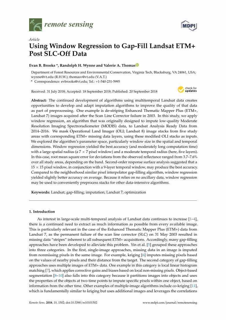
Figure 5. Examples of window regression outputs. A poor fit (left) is shown in the Alaska study area, Band 1 (Ultra Blue), with parameters = 1, = 3, and = 5. A good fit (right) is shown in the Arizona study area, Band 5 (Near Infrared), with parameters = 3, = 2, and = 5.

Table 4. ANOVA main effects and interactions for window regression accuracy and processing time, with the mean absolute percentage error (MAPE) over the imputed stack and run times as the responses. Statistically significant effects (5% level) are marked with an X.

Factor MAPE Run Time Study Area X X *

Band X r X X t X m X

r × Study Area X X * r × Band

r × t X r × m X t × m

* Artifacts of extended processing time.

Figure 5. Examples of window regression outputs. A poor fit (left) is shown in the Alaska study area,Band 1 (Ultra Blue), with parameters r = 1, t = 3, and m = 5. A good fit (right) is shown in the Arizonastudy area, Band 5 (Near Infrared), with parameters r = 3, t = 2, and m = 5.

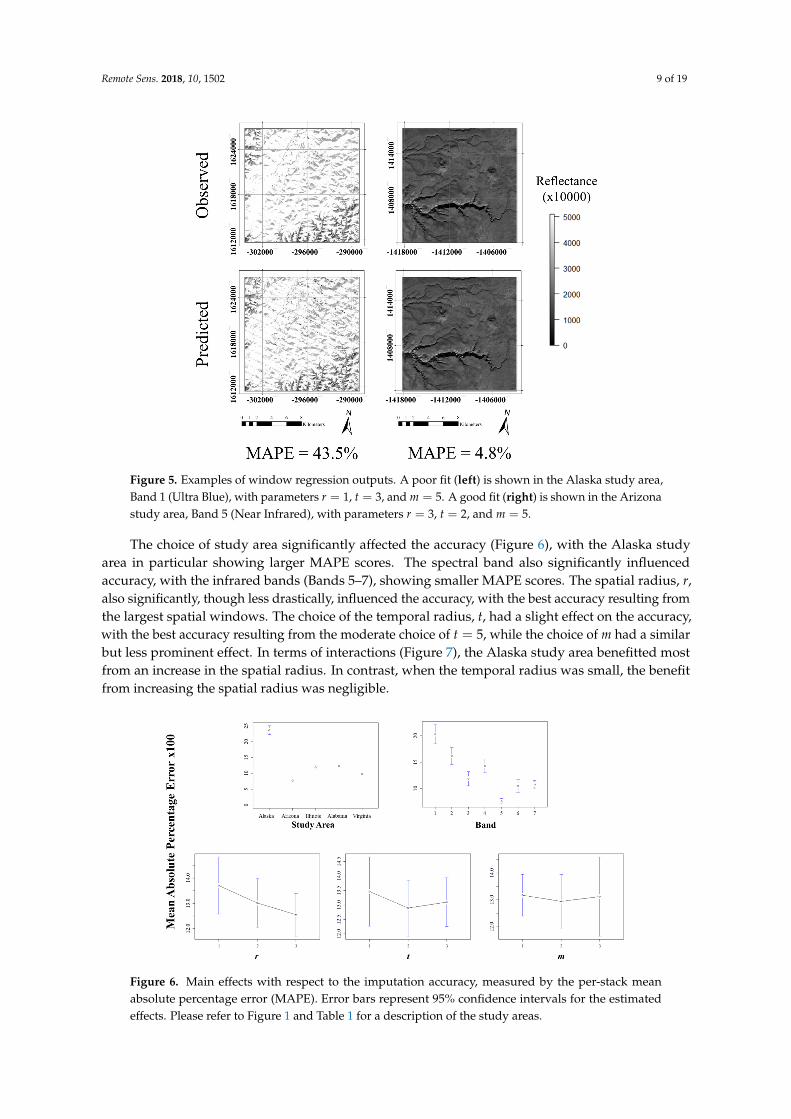
The choice of study area significantly affected the accuracy (Figure 6), with the Alaska studyarea in particular showing larger MAPE scores. The spectral band also significantly influencedaccuracy, with the infrared bands (Bands 5–7), showing smaller MAPE scores. The spatial radius, r,also significantly, though less drastically, influenced the accuracy, with the best accuracy resulting fromthe largest spatial windows. The choice of the temporal radius, t, had a slight effect on the accuracy,with the best accuracy resulting from the moderate choice of t = 5, while the choice of m had a similarbut less prominent effect. In terms of interactions (Figure 7), the Alaska study area benefitted mostfrom an increase in the spatial radius. In contrast, when the temporal radius was small, the benefitfrom increasing the spatial radius was negligible.

Remote Sens. 2018, 10, x FOR PEER REVIEW 10 of 20

The choice of study area significantly affected the accuracy (Figure 6), with the Alaska study area in particular showing larger MAPE scores. The spectral band also significantly influenced accuracy, with the infrared bands (Bands 5–7), showing smaller MAPE scores. The spatial radius, r, also significantly, though less drastically, influenced the accuracy, with the best accuracy resulting from the largest spatial windows. The choice of the temporal radius, t, had a slight effect on the accuracy, with the best accuracy resulting from the moderate choice of = 5, while the choice of m had a similar but less prominent effect. In terms of interactions (Figure 7), the Alaska study area benefitted most from an increase in the spatial radius. In contrast, when the temporal radius was small, the benefit from increasing the spatial radius was negligible.

Figure 6. Main effects with respect to the imputation accuracy, measured by the per-stack mean absolute percentage error (MAPE). Error bars represent 95% confidence intervals for the estimated effects. Please refer to Figure 1 and Table 1 for a description of the study areas.

Figure 7. Statistically significant (5% level) interaction effects with respect to the imputation accuracy, measured by per-stack mean absolute percentage error (MAPE). Please refer to Figure 1 and Table 1 for a description of the study areas.

With respect to the processing time (Figure 8), we used the recorded processing time divided by the shortest processing time of all the combinations: in this case, the stack from Band 1 in Alaska, with a parameter combination of = 1, = 3, and = 5. Parallelizing on eight logical processors, this run took 321 s (~5.4 min) to complete. We observed an increase in the run time over iterations of

Figure 6. Main effects with respect to the imputation accuracy, measured by the per-stack meanabsolute percentage error (MAPE). Error bars represent 95% confidence intervals for the estimatedeffects. Please refer to Figure 1 and Table 1 for a description of the study areas.

Remote Sens. 2018, 10, 1502 10 of 19

Remote Sens. 2018, 10, x FOR PEER REVIEW 10 of 20

The choice of study area significantly affected the accuracy (Figure 6), with the Alaska study area in particular showing larger MAPE scores. The spectral band also significantly influenced accuracy, with the infrared bands (Bands 5–7), showing smaller MAPE scores. The spatial radius, r, also significantly, though less drastically, influenced the accuracy, with the best accuracy resulting from the largest spatial windows. The choice of the temporal radius, t, had a slight effect on the accuracy, with the best accuracy resulting from the moderate choice of = 5, while the choice of m had a similar but less prominent effect. In terms of interactions (Figure 7), the Alaska study area benefitted most from an increase in the spatial radius. In contrast, when the temporal radius was small, the benefit from increasing the spatial radius was negligible.

Figure 6. Main effects with respect to the imputation accuracy, measured by the per-stack mean absolute percentage error (MAPE). Error bars represent 95% confidence intervals for the estimated effects. Please refer to Figure 1 and Table 1 for a description of the study areas.

Figure 7. Statistically significant (5% level) interaction effects with respect to the imputation accuracy, measured by per-stack mean absolute percentage error (MAPE). Please refer to Figure 1 and Table 1 for a description of the study areas.

With respect to the processing time (Figure 8), we used the recorded processing time divided by the shortest processing time of all the combinations: in this case, the stack from Band 1 in Alaska, with a parameter combination of = 1, = 3, and = 5. Parallelizing on eight logical processors, this run took 321 s (~5.4 min) to complete. We observed an increase in the run time over iterations of

Figure 7. Statistically significant (5% level) interaction effects with respect to the imputation accuracy,measured by per-stack mean absolute percentage error (MAPE). Please refer to Figure 1 and Table 1 fora description of the study areas.

With respect to the processing time (Figure 8), we used the recorded processing time dividedby the shortest processing time of all the combinations: in this case, the stack from Band 1 in Alaska,with a parameter combination of r = 1, t = 3, and m = 5. Parallelizing on eight logical processors,this run took 321 s (~5.4 min) to complete. We observed an increase in the run time over iterations ofstudy area, despite each study area being chosen to have the same extent and layer count. The slowestrun resulted from using the Band 1 stack in Virginia with a parameter combination of r = 3, t = 3,and m = 7; this run took 1983 s (~33.1 min) to complete. This suggests computer fatigue from theprocessing. Accounting for this, we still observed that the run time increased exponentially both withthe choice of r and with choice of m, while the run time decreased as t increased. There was onestatistically significant interaction effect between r and m (Figure 9), showing a slight increase in theprocessing time as both the spatial radius and the minimum required pairs increased.

Remote Sens. 2018, 10, x FOR PEER REVIEW 11 of 20

study area, despite each study area being chosen to have the same extent and layer count. The slowest run resulted from using the Band 1 stack in Virginia with a parameter combination of = 3, = 3, and = 7; this run took 1983 s (~33.1 min) to complete. This suggests computer fatigue from the processing. Accounting for this, we still observed that the run time increased exponentially both with the choice of r and with choice of m, while the run time decreased as t increased. There was one statistically significant interaction effect between r and m (Figure 9), showing a slight increase in the processing time as both the spatial radius and the minimum required pairs increased.

Figure 8. Main effects with respect to run time, denoted by multipliers of the minimum observed processing time. Error bars represent 95% confidence intervals for the estimated effects. Please refer to Figure 1 and Table 1 for a description of the study areas.

Figure 9. Interaction of the spatial radius, r, and the minimum-pairs parameter, m, with respect to the run time, as denoted by multipliers of the minimum observed processing time. Please refer to Figure 1 and Table 1 for a description of the study areas.

3.2. Optimization

Although the study area and the spectral band each had significant impacts on the imputation accuracy, for general application, we were most interested in the parameter combinations that

Figure 8. Main effects with respect to run time, denoted by multipliers of the minimum observedprocessing time. Error bars represent 95% confidence intervals for the estimated effects. Please refer toFigure 1 and Table 1 for a description of the study areas.

Remote Sens. 2018, 10, 1502 11 of 19

Remote Sens. 2018, 10, x FOR PEER REVIEW 11 of 20

study area, despite each study area being chosen to have the same extent and layer count. The slowest run resulted from using the Band 1 stack in Virginia with a parameter combination of = 3, = 3, and = 7; this run took 1983 s (~33.1 min) to complete. This suggests computer fatigue from the processing. Accounting for this, we still observed that the run time increased exponentially both with the choice of r and with choice of m, while the run time decreased as t increased. There was one statistically significant interaction effect between r and m (Figure 9), showing a slight increase in the processing time as both the spatial radius and the minimum required pairs increased.

Figure 8. Main effects with respect to run time, denoted by multipliers of the minimum observed processing time. Error bars represent 95% confidence intervals for the estimated effects. Please refer to Figure 1 and Table 1 for a description of the study areas.

Figure 9. Interaction of the spatial radius, r, and the minimum-pairs parameter, m, with respect to the run time, as denoted by multipliers of the minimum observed processing time. Please refer to Figure 1 and Table 1 for a description of the study areas.

3.2. Optimization

Although the study area and the spectral band each had significant impacts on the imputation accuracy, for general application, we were most interested in the parameter combinations that

Figure 9. Interaction of the spatial radius, r, and the minimum-pairs parameter, m, with respect to therun time, as denoted by multipliers of the minimum observed processing time. Please refer to Figure 1and Table 1 for a description of the study areas.

3.2. Optimization

Although the study area and the spectral band each had significant impacts on the imputationaccuracy, for general application, we were most interested in the parameter combinations that yieldedan optimal tradeoff between the accuracy and the processing time. Figure 10 shows the second-orderresponse surfaces based on our exploration for both MAPE and run time, with respect to r and t.(We chose t instead of m because m is constrained by the choice of t.) The influence of r was obvious,with a clear indication that greater accuracy might be achieved with greater values of r than thosetested here, at the cost of longer run times. The choice of t was not as great an influence, but thesurfaces suggested a “sweet spot” when t was 2 or 3. In terms of the canonical paths of steepest descent,the response surfaces pointed toward conflicting minima: a minimum MAPE when r = 7 and t = 4,and a minimum run time when r = 1 and t = 2.

Remote Sens. 2018, 10, x FOR PEER REVIEW 12 of 20

yielded an optimal tradeoff between the accuracy and the processing time. Figure 10 shows the second-order response surfaces based on our exploration for both MAPE and run time, with respect to r and t. (We chose t instead of m because m is constrained by the choice of t.) The influence of r was obvious, with a clear indication that greater accuracy might be achieved with greater values of r than those tested here, at the cost of longer run times. The choice of t was not as great an influence, but the surfaces suggested a “sweet spot” when t was 2 or 3. In terms of the canonical paths of steepest descent, the response surfaces pointed toward conflicting minima: a minimum MAPE when = 7 and = 4, and a minimum run time when = 1 and = 2.

Figure 10. Second-order response surfaces for accuracy (left) and run time (right) with respect to choice of spatial radius, r, and temporal radius, t.

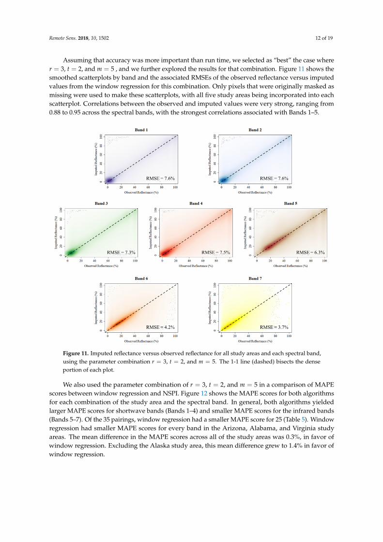
Assuming that accuracy was more important than run time, we selected as “best” the case where = 3, = 2, and = 5 , and we further explored the results for that combination. Figure 11 shows the smoothed scatterplots by band and the associated RMSEs of the observed reflectance versus imputed values from the window regression for this combination. Only pixels that were originally masked as missing were used to make these scatterplots, with all five study areas being incorporated into each scatterplot. Correlations between the observed and imputed values were very strong, ranging from 0.88 to 0.95 across the spectral bands, with the strongest correlations associated with Bands 1–5.

We also used the parameter combination of = 3, = 2, and = 5 in a comparison of MAPE scores between window regression and NSPI. Figure 12 shows the MAPE scores for both algorithms for each combination of the study area and the spectral band. In general, both algorithms yielded larger MAPE scores for shortwave bands (Bands 1–4) and smaller MAPE scores for the infrared bands (Bands 5–7). Of the 35 pairings, window regression had a smaller MAPE score for 25 (Table 5). Window regression had smaller MAPE scores for every band in the Arizona, Alabama, and Virginia study areas. The mean difference in the MAPE scores across all of the study areas was 0.3%, in favor of window regression. Excluding the Alaska study area, this mean difference grew to 1.4% in favor of window regression.

Figure 10. Second-order response surfaces for accuracy (left) and run time (right) with respect tochoice of spatial radius, r, and temporal radius, t.

Remote Sens. 2018, 10, 1502 12 of 19

Assuming that accuracy was more important than run time, we selected as “best” the case wherer = 3, t = 2, and m = 5 , and we further explored the results for that combination. Figure 11 shows thesmoothed scatterplots by band and the associated RMSEs of the observed reflectance versus imputedvalues from the window regression for this combination. Only pixels that were originally masked asmissing were used to make these scatterplots, with all five study areas being incorporated into eachscatterplot. Correlations between the observed and imputed values were very strong, ranging from0.88 to 0.95 across the spectral bands, with the strongest correlations associated with Bands 1–5.Remote Sens. 2018, 10, x FOR PEER REVIEW 13 of 20

Figure 11. Imputed reflectance versus observed reflectance for all study areas and each spectral band, using the parameter combination = 3, = 2, and = 5. The 1-1 line (dashed) bisects the dense portion of each plot.

Figure 12. Overall mean absolute percentage error (MAPE) scores for all image stacks, for the Neighborhood Similar Pixel Interpolator (NSPI) and window regression (using a parameter combination of = 3, = 2, and = 5). Symbols below the 1-1 line (dashed) represent the study area/band combinations for which window regression had a smaller MAPE score than NSPI.

Figure 11. Imputed reflectance versus observed reflectance for all study areas and each spectral band,using the parameter combination r = 3, t = 2, and m = 5. The 1-1 line (dashed) bisects the denseportion of each plot.

We also used the parameter combination of r = 3, t = 2, and m = 5 in a comparison of MAPEscores between window regression and NSPI. Figure 12 shows the MAPE scores for both algorithmsfor each combination of the study area and the spectral band. In general, both algorithms yieldedlarger MAPE scores for shortwave bands (Bands 1–4) and smaller MAPE scores for the infrared bands(Bands 5–7). Of the 35 pairings, window regression had a smaller MAPE score for 25 (Table 5). Windowregression had smaller MAPE scores for every band in the Arizona, Alabama, and Virginia studyareas. The mean difference in the MAPE scores across all of the study areas was 0.3%, in favor ofwindow regression. Excluding the Alaska study area, this mean difference grew to 1.4% in favor ofwindow regression.

Remote Sens. 2018, 10, 1502 13 of 19

Remote Sens. 2018, 10, x FOR PEER REVIEW 13 of 20

Figure 11. Imputed reflectance versus observed reflectance for all study areas and each spectral band, using the parameter combination = 3, = 2, and = 5. The 1-1 line (dashed) bisects the dense portion of each plot.

Figure 12. Overall mean absolute percentage error (MAPE) scores for all image stacks, for the Neighborhood Similar Pixel Interpolator (NSPI) and window regression (using a parameter combination of = 3, = 2, and = 5). Symbols below the 1-1 line (dashed) represent the study area/band combinations for which window regression had a smaller MAPE score than NSPI.

Figure 12. Overall mean absolute percentage error (MAPE) scores for all image stacks, for theNeighborhood Similar Pixel Interpolator (NSPI) and window regression (using a parameter combinationof r = 3, t = 2, and m = 5). Symbols below the 1-1 line (dashed) represent the study area/bandcombinations for which window regression had a smaller MAPE score than NSPI.

Table 5. Combinations used when comparing window regression and the Neighborhood Similar PixelInterpolator (NSPI). Combinations for which the mean absolute percentage error (MAPE) scores forwindow regression were less than those of NSPI are marked with an X.

Band Alaska Arizona Illinois Alabama Virginia

1 X X X2 X X X3 X X X4 X X X5 X X X X X6 X X X X7 X X X X

4. Discussion

We assessed window regression along two responses: (1) overall accuracy, represented by themean absolute percentage error (MAPE), and (2) the processing time, as represented by multiples of theshortest run made in this study. Most of the results conformed to our expectations. As the spatial radiusincreased, the overall accuracy increased, but it came at the cost of exponentially longer run times.The middle value for the temporal radius, corresponding to a window depth of five layers, producedthe best overall accuracy. The minimum-pairs parameter had no strong effect on accuracy but, like thespatial radius, led to exponentially longer run times as it increased. Taken together, these resultssuggest that large windows with a moderate timeframe produce the best overall imputation, providedone is able to mitigate the computational costs.

Window regression imputes the missing data for a pixel by comparing that pixel with its spatialneighbors for a temporal subset. The neighboring pixel with the maximum absolute correlation to thetarget pixel is used to impute the pixel, but there is no inherent constraint on the quality of this match.In our example pixel (Figure 4), one date was very poorly imputed. Of the original 48 neighboringpixels to consider, only seven had values for this date. These pixels were all at the edge of the spatialwindow, implying a weaker correlation and thus poorer imputation (which was borne out in the

Remote Sens. 2018, 10, 1502 14 of 19

analysis). This is a disadvantage of window regression: it will impute data based on existing data,even if that data is sparse. This issue makes it more difficult for window regression to impute broadareas of missing data, since the quality of said imputations depends on how well the interior areamatches with the edge. One might rectify this by introducing a new parameter akin to the minimumpairs parameter, m, but a simpler solution is to place a threshold on the correlation. If the absolutecorrelation between the target pixel and all candidates falls below this threshold, then let the algorithmignore this pixel for the current iteration. As the neighboring pixels are imputed, the quality of matchesshould generally increase (though there is propagation of error to consider) and provide additional,better chances for imputing the target pixel at the cost of possibly not being able to impute all of thepixels. Alternatively, one might use a raster of the correlations associated with the imputations as aquality metric. We have implemented this adjustment by adding a minimum absolute correlationthreshold in the R code available with this article, though we did not employ it for the main study.

In terms of accuracy, we found that window regression was strongly sensitive to the study areaand the spectral band chosen (Figure 6), both of which imply that window regression performs better(or worse) on different land covers and spectral ranges. With respect to the spectrum, we note thatbecause shorter-wavelength bands such as Ultra Blue and Blue (Bands 1 and 2, respectively) aretypically darker, our use of percentage error most likely exaggerated the imputation error for thesebands. This is supported by observing that the correlations between observed and imputed values forthe case of r = 3, t = 2, and m = 5 (Figure 11) are greatest for these bands. With respect to the studyarea, the median MAPE score for the Alaska area was 23.30%, while the next greatest median MAPEwas 11.9% for the Alabama area. We postulate that in the Alaska area, the combination of saturatedpixels due to snow, along with the unfortunate coincidence that the ETM+ stripes appear to alignwith much of the topography (Figure 13), prompted much of the poor performance. The timeframecovered in each study area was at least one year, so it is possible that certain seasonal effects mayhave contributed to poorer imputation in some areas. We note that the Arizona study area, which hadminimal vegetation and snow effects, was the area for which window regression yielded the smallestMAPE scores. In general, gap-filling algorithms should perform better on a static landscape becausethere is less variation between images and thus less room for error in imputation.

Remote Sens. 2018, 10, x FOR PEER REVIEW 15 of 20

timeframe covered in each study area was at least one year, so it is possible that certain seasonal effects may have contributed to poorer imputation in some areas. We note that the Arizona study area, which had minimal vegetation and snow effects, was the area for which window regression yielded the smallest MAPE scores. In general, gap-filling algorithms should perform better on a static landscape because there is less variation between images and thus less room for error in imputation.

Figure 13. Hillshaded relief of the Alaska study area based on interferometric synthetic aperture radar (IFSAR) data [36], with ETM+ missing data stripes from one acquisition date overlaid in red. Note the tendency for the stripes to align with topographical features (black arrow).

A related question is how well window regression can handle changes to land cover and/or land use. For example, if the pixel being imputed undergoes an abrupt change, what effect might we expect this to have on the imputation? Window regression considers only the neighboring pixel with maximal absolute correlation, over a temporal window that reaches both before and after the change. This pairwise correlation is computed without regard to the particular timing of values, so as long as both pixels exhibit similar trajectories the correlation should remain strong. Thus, we expect that if there is another pixel in the neighborhood that has undergone a similar change (e.g., if both pixels underwent a common land use change), the algorithm would still impute effectively, possibly with even more accuracy than other methods (aside from local linear histogram matching [7], which would similarly be trajectory-invariant). Conversely, if there are no available neighboring pixels that undergo a similar change (e.g., the only pixels with nonmissing data on the target date did not undergo any changes), we expect window regression to perform poorly. Thus, if the area of typical land use changes is generally larger than the area being imputed (e.g., if forested lots are typically larger than ETM+ stripes), window regression should perform well.

The MAPE scores for all bands and combinations ranged from 4.7% to 43.5%, with the interquartile scores falling between 7.9% and 15.9%. In the case study of = 3, = 2, and = 5, we found RMSE values ranging from 3.7% to 7.6% reflectance by spectral band. These values are slightly higher than those found by Yin et al. ([5]; Table 5) in their comparison of gap-filling algorithms for heterogeneous areas, but they are within the same order of magnitude. In our comparison with the NSPI gap-filling algorithm using the same image stacks, we found that window regression produced slightly smaller MAPE scores over all study areas (Figure 12). Window regression produced smaller MAPE scores for all bands in three of the five study areas. While the differences in MAPE scores

Figure 13. Hillshaded relief of the Alaska study area based on interferometric synthetic aperture radar(IFSAR) data [36], with ETM+ missing data stripes from one acquisition date overlaid in red. Note thetendency for the stripes to align with topographical features (black arrow).

Remote Sens. 2018, 10, 1502 15 of 19

A related question is how well window regression can handle changes to land cover and/orland use. For example, if the pixel being imputed undergoes an abrupt change, what effect might weexpect this to have on the imputation? Window regression considers only the neighboring pixel withmaximal absolute correlation, over a temporal window that reaches both before and after the change.This pairwise correlation is computed without regard to the particular timing of values, so as longas both pixels exhibit similar trajectories the correlation should remain strong. Thus, we expect thatif there is another pixel in the neighborhood that has undergone a similar change (e.g., if both pixelsunderwent a common land use change), the algorithm would still impute effectively, possibly witheven more accuracy than other methods (aside from local linear histogram matching [7], which wouldsimilarly be trajectory-invariant). Conversely, if there are no available neighboring pixels that undergoa similar change (e.g., the only pixels with nonmissing data on the target date did not undergo anychanges), we expect window regression to perform poorly. Thus, if the area of typical land use changesis generally larger than the area being imputed (e.g., if forested lots are typically larger than ETM+stripes), window regression should perform well.

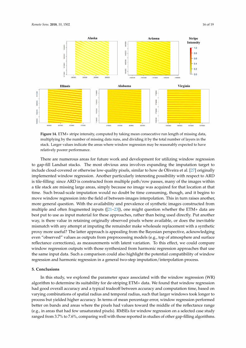
The MAPE scores for all bands and combinations ranged from 4.7% to 43.5%, with the interquartilescores falling between 7.9% and 15.9%. In the case study of r = 3, t = 2, and m = 5, we found RMSEvalues ranging from 3.7% to 7.6% reflectance by spectral band. These values are slightly higher thanthose found by Yin et al. ([5]; Table 5) in their comparison of gap-filling algorithms for heterogeneousareas, but they are within the same order of magnitude. In our comparison with the NSPI gap-fillingalgorithm using the same image stacks, we found that window regression produced slightly smallerMAPE scores over all study areas (Figure 12). Window regression produced smaller MAPE scoresfor all bands in three of the five study areas. While the differences in MAPE scores between windowregression and NSPI were relatively small, the results taken together with Yin et al. [5] do suggestthat window regression performs at least as well as current gap-filling algorithms. In terms of generalperformance, we can reasonably expect window regression to perform better in practice than in thisstudy, primarily because here, we effectively used a collection of data corresponding to an ETM+-onlyscenario. Since window regression relies on having nonmissing data within a temporal radius of anygiven layer, it may be expected to perform more poorly when the ETM+ stripes are geographicallyconsistent (i.e., in the off-nadir areas of the scene). We can assess the impact this might have hadin our study (Figure 14) by observing the density (e.g., consecutive run length) of missing data,multiplied by the number of missing data runs and dividing by the number of layers to make anindex of striping intensity. In the extreme case, an intensity of 1 states that every instance of the targetpixel is missing; thus, it cannot be imputed. While this intensity is hardly the sole driver of windowregression’s performance (note the relatively low intensity in the Alaska area, which had the largestoverall MAPE scores) and we did not perform a full analysis of such intensity against imputationerror, we might expect that incorporating contemporary TM (Landsat 4–5) or OLI (Landsat 8) imageryinto an ETM+ stack will improve the overall performance, provided that within-band correlationsbetween the various sensors remain consistent. Similarly, we note that the maximum spatial radiusconsidered in this study resulted in a 7 × 7 pixel window. In this study, we observed ETM+ stripesas wide as 13 pixels. Thus, even with our maximum spatial radius, window regression could notimpute an entire image stack in one iteration. Increasing the spatial radius to r = 7, the optimalvalue suggested by the response surface analysis (Figure 10), would enable a single-iteration run inthis case. However, the greater (and potentially extreme) distance to the target pixel could reducethe quality of the imputation, as in the example pixel shown in Figure 4. Employing a minimumcorrelation threshold as suggested in this discussion could mitigate this effect and preserve accuracywhile improving computational speed.

Remote Sens. 2018, 10, 1502 16 of 19

Remote Sens. 2018, 10, x FOR PEER REVIEW 16 of 20

between window regression and NSPI were relatively small, the results taken together with Yin et al. [5] do suggest that window regression performs at least as well as current gap-filling algorithms. In terms of general performance, we can reasonably expect window regression to perform better in practice than in this study, primarily because here, we effectively used a collection of data corresponding to an ETM+-only scenario. Since window regression relies on having nonmissing data within a temporal radius of any given layer, it may be expected to perform more poorly when the ETM+ stripes are geographically consistent (i.e., in the off-nadir areas of the scene). We can assess the impact this might have had in our study (Figure 14) by observing the density (e.g., consecutive run length) of missing data, multiplied by the number of missing data runs and dividing by the number of layers to make an index of striping intensity. In the extreme case, an intensity of 1 states that every instance of the target pixel is missing; thus, it cannot be imputed. While this intensity is hardly the sole driver of window regression’s performance (note the relatively low intensity in the Alaska area, which had the largest overall MAPE scores) and we did not perform a full analysis of such intensity against imputation error, we might expect that incorporating contemporary TM (Landsat 4–5) or OLI (Landsat 8) imagery into an ETM+ stack will improve the overall performance, provided that within-band correlations between the various sensors remain consistent. Similarly, we note that the maximum spatial radius considered in this study resulted in a 7 × 7 pixel window. In this study, we observed ETM+ stripes as wide as 13 pixels. Thus, even with our maximum spatial radius, window regression could not impute an entire image stack in one iteration. Increasing the spatial radius to = 7, the optimal value suggested by the response surface analysis (Figure 10), would enable a single-iteration run in this case. However, the greater (and potentially extreme) distance to the target pixel could reduce the quality of the imputation, as in the example pixel shown in Figure 4. Employing a minimum correlation threshold as suggested in this discussion could mitigate this effect and preserve accuracy while improving computational speed.

Figure 14. ETM+ stripe intensity, computed by taking mean consecutive run length of missing data, multiplying by the number of missing data runs, and dividing it by the total number of layers in the stack. Larger values indicate the areas where window regression may be reasonably expected to have relatively poorer performance.

There are numerous areas for future work and development for utilizing window regression to gap-fill Landsat stacks. The most obvious area involves expanding the imputation target to include cloud-covered or otherwise low-quality pixels, similar to how de Oliveira et al. [27] originally implemented window regression. Another particularly interesting possibility with respect to ARD is tile-filling: since ARD is constructed from multiple path/row passes, many of the images within a tile

Figure 14. ETM+ stripe intensity, computed by taking mean consecutive run length of missing data,multiplying by the number of missing data runs, and dividing it by the total number of layers in thestack. Larger values indicate the areas where window regression may be reasonably expected to haverelatively poorer performance.

There are numerous areas for future work and development for utilizing window regressionto gap-fill Landsat stacks. The most obvious area involves expanding the imputation target toinclude cloud-covered or otherwise low-quality pixels, similar to how de Oliveira et al. [27] originallyimplemented window regression. Another particularly interesting possibility with respect to ARDis tile-filling: since ARD is constructed from multiple path/row passes, many of the images withina tile stack are missing large areas, simply because no image was acquired for that location at thattime. Such broad-scale imputation would no doubt be time consuming, though, and it begins tomove window regression into the field of between-images interpolation. This in turn raises another,more general question. With the availability and prevalence of synthetic images constructed frommultiple and often fragmented inputs ([21–23]), one might question whether the ETM+ data arebest put to use as input material for these approaches, rather than being used directly. Put anotherway, is there value in retaining originally observed pixels where available, or does the inevitablemismatch with any attempt at imputing the remainder make wholesale replacement with a syntheticproxy more useful? The latter approach is appealing from the Bayesian perspective, acknowledgingeven “observed” values as outputs from preprocessing models (e.g., top of atmosphere and surfacereflectance corrections), as measurements with latent variation. To this effect, we could comparewindow regression outputs with those synthesized from harmonic regression approaches that usethe same input data. Such a comparison could also highlight the potential compatibility of windowregression and harmonic regression in a general two-step imputation/interpolation process.

5. Conclusions

In this study, we explored the parameter space associated with the window regression (WR)algorithm to determine its suitability for de-striping ETM+ data. We found that window regressionhad good overall accuracy and a typical tradeoff between accuracy and computation time, based onvarying combinations of spatial radius and temporal radius, such that larger windows took longer toprocess but yielded higher accuracy. In terms of mean percentage error, window regression performedbetter on bands and areas where the pixels had values toward the middle of the reflectance range(e.g., in areas that had few unsaturated pixels). RMSEs for window regression on a selected case studyranged from 3.7% to 7.6%, comparing well with those reported in studies of other gap-filling algorithms.

Remote Sens. 2018, 10, 1502 17 of 19

We found that using larger spatial window sizes resulted in better accuracy, with an optimal spatialradius of r = 7 suggested by response surface analysis. In a direct comparison between windowregression and another gap-filling algorithm, window regression yielded slightly better accuracy whenaveraging over all spectral bands and study areas.

In general, window regression has the advantages of self-containment and simplicity: it inputsa stack of images with missing data, and then it uses only that stack and a combination of linearmodels to output an image stack with the missing values imputed. Window regression can bereiterated, with each successive pass imputing more of the original stack, until the stack has little tono missing data remaining. However, window regression can only impute based on available data.If a missing pixel has only dissimilar pixels with which to compare, window regression risks a poorimputation. Additionally, pixels imputed in successive iterations may suffer error propagation effects.Increasing the spatial window size mitigates these effects and improves accuracy, at the cost of longercomputation time. Finally, window regression is a within-images gap-filling method, fundamentallyunlike harmonic regression and other between-images interpolation algorithms. Accordingly, windowregression has the potential to be improve the quality of inputs for such methods and their downstreamresidual analyses.

Author Contributions: Conceptualization, E.B.B., R.H.W., and V.A.T.; Methodology, E.B.B., R.H.W., and V.A.T.;Software, E.B.B.; Validation, E.B.B., R.H.W., and V.A.T.; Formal Analysis, E.B.B.; Investigation, E.B.B.; Resources,E.B.B.; Data Curation, E.B.B.; Writing—Original Draft Preparation, E.B.B.; Writing—Review & Editing, E.B.B.,R.H.W., and V.A.T.; Visualization, E.B.B.; Supervision, R.H.W. and V.A.T.; Project Administration, E.B.B.; FundingAcquisition, R.H.W. and V.A.T.

Funding: This research was funded in part by the RPA Land Use Modeling Grant/Contract ID 14-JV-11330145-108,funded by the USDA Forest Service. Funding for R.H.W.’s and V.A.T.’s participation was also provided by theVirginia Agricultural Experiment Station and the McIntire-Stennis Program of NIFA, USDA (Project Number1007054, “Detecting and Forecasting the Consequences of Subtle and Gross Disturbance on Forest CarbonCycling”). The APC was discounted by institutional membership with MDPI through the Virginia Tech library.

Acknowledgments: The authors gratefully acknowledge the constructive feedback of the three independentpeer reviewers.

Conflicts of Interest: The authors declare no conflict of interest.

Appendix A

Additional details regarding the five study areas and Landsat images used in this study arepresented in Table A1.

Table A1. Image acquisition dates for each study area. AK and CU reference the Alaska and ContiguousUSA Albers Equal Area Conic projections, respectively. Note that candidate images for the 2014-2018period were downloaded, but only the first 24 high-quality images from each stack were used inthe analysis.

Study Area ARD Tile Acquisition Year Acquisition Date

WesternAlaska AK h3v5

2014 2/21, 3/9, 3/16, 3/25, 4/1, 4/10, 4/26, 5/19, 8/23, 9/8, 9/24, 10/32015 3/12, 3/19, 4/4, 4/20, 4/29, 5/6, 5/31, 6/16, 6/232016 3/5, 3/21, 3/30

CentralArizona

CU h7v122014 1/12, 3/17, 5/4, 5/20, 6/5, 6/21, 7/23, 8/8, 10/11, 10/27, 11/12,

11/28, 12/14, 12/302015 1/15, 2/16, 3/4, 3/20, 4/5, 4/21, 5/7, 6/8, 6/24, 7/10

East CentralIllinois

CU h21v92014 1/19, 2/11, 2/27, 3/15, 4/9, 4/16, 4/25, 5/11, 5/18, 6/3, 7/21,

7/30, 10/25, 11/32015 1/13, 2/7, 2/23, 3/11, 4/28, 5/5, 8/2, 8/25, 9/3, 10/21

West CentralAlabama

CU h22v142014 1/12, 2/13, 3/10, 3/26, 5/4, 5/20, 7/7, 7/16, 8/8, 8/24, 9/25,

10/4, 10/27, 11/21, 11/28, 12/72015 1/8, 1/31, 4/21, 4/30, 5/7, 5/23, 6/17, 7/10

CentralVirginia CU h27v10

2014 1/9, 1/18, 3/14, 4/24, 5/17, 5/26, 6/2, 6/11, 6/18, 6/27, 7/4,7/29, 8/14, 8/21, 9/6, 9/22, 10/8, 10/17, 12/11, 12/27

2015 1/5, 1/28, 2/6, 2/13

Remote Sens. 2018, 10, 1502 18 of 19

References

1. Loveland, T.R.; Dwyer, J.L. Landsat: building a strong future. Remote Sens. Environ. 2012, 122, 22–29.[CrossRef]

2. Markham, B.L.; Helder, D.L. Forty-year calibrated record of earth-reflected radiance from Landsat: A review.Remote Sens. Environ. 2012, 122, 30–40. [CrossRef]

3. Wulder, M.A.; White, J.C.; Loveland, T.R.; Woodcock, C.E.; Belward, A.S.; Cohen, W.B.; Fosnight, E.A.; Shaw, J.;Masek, J.G.; Roy, D.P. The global Landsat archive: status, consolidation, and direction. Remote Sens. Environ.2016, 185, 271–283. [CrossRef]

4. Zhu, Z. Change detection using landsat time series: A review of frequencies, preprocessing, algorithms,and applications. ISPRS J. Photogramm. 2017, 130, 370–384. [CrossRef]

5. Yin, G.; Mariethoz, G.; Sun, Y.; McCabe, M.F. A comparison of gap-filling approaches for Landsat-7satellite data. Int. J. Remote Sens. 2017, 38, 6653–6679. [CrossRef]

6. Zhang, C.; Li, W.; Travis, D. Gaps-fill of SLC-off Landsat ETM+ satellite image using a geostatistical approach.Int. J. Remote Sens. 2007, 28, 5103–5122. [CrossRef]

7. Scaramuzza, P.; Micijevic, E.; Chander, G. SLC Gap-Filled Products Phase One Methodology. Availableonline: https://on.doi.gov/2QEVyGy (accessed on 18 September 2018).

8. Maxwell, S. Filling Landsat ETM+ SLC-off gaps using a segmentation model approach. Photogramm. Eng.Remote Sens. 2004, 70, 1109–1112.

9. Maxwell, S.; Schmidt, G.; Storey, J. A multi-scale segmentation approach to filling gaps in Landsat ETM+SLC-off images. Int. J. Remote Sens. 2007, 28, 5339–5356. [CrossRef]

10. Zheng, B.; Campbell, J.B.; Shao, Y.; Wynne, R.H. Broad-scale monitoring of tillage practices using sequentialLandsat imagery. Soil Sci. Soc. Am. J. 2013, 77, 1755–1764. [CrossRef]

11. Pringle, M.; Schmidt, M.; Muir, J. Geostatistical interpolation of SLC-off Landsat ETM+ images. ISPRS J.Photogramm 2009, 64, 654–664. [CrossRef]

12. Chen, J.; Zhu, X.; Vogelmann, J.E.; Gao, F.; Jin, S. A simple and effective method for filling gaps in LandsatETM+ SLC-off images. Remote Sens. Environ. 2011, 115, 1053–1064. [CrossRef]

13. Zhu, X.; Liu, D.; Chen, J. A new geostatistical approach for filling gaps in Landsat ETM+ SLC-off images.Remote Sens. Environ. 2012, 124, 49–60. [CrossRef]

14. Malambo, L.; Heatwole, C.D. A multitemporal profile-based interpolation method for gap fillingnonstationary data. IEEE Trans. Geosci. Remote 2016, 54, 252–261. [CrossRef]

15. Roy, D.P.; Ju, J.; Lewis, P.; Schaaf, C.; Gao, F.; Hansen, M.; Lindquist, E. Multi-temporal MODIS–Landsatdata fusion for relative radiometric normalization, gap filling, and prediction of Landsat data.Remote Sens. Environ. 2008, 112, 3112–3130. [CrossRef]

16. Wijedasa, L.S.; Sloan, S.; Michelakis, D.G.; Clements, G.R. Overcoming limitations with Landsat imagery formapping of peat swamp forests in Sundaland. Remote Sens. 2012, 4, 2595–2618. [CrossRef]

17. Wulder, M.A.; Masek, J.G.; Cohen, W.B.; Loveland, T.R.; Woodcock, C.E. Opening the archive: How freedata has enabled the science and monitoring promise of Landsat. Remote Sens. Environ. 2012, 122, 2–10.[CrossRef]

18. Brooks, E.B.; Coulston, J.W.; Wynne, R.H.; Thomas, V.A. Improving the precision of dynamic forest parameterestimates using Landsat. Remote Sens. Environ. 2016, 179, 162–169. [CrossRef]

19. Cohen, W.; Healey, S.; Yang, Z.; Stehman, S.; Brewer, C.; Brooks, E.; Gorelick, N.; Huang, C.; Hughes, M.;Kennedy, R.; et al. How similar are forest disturbance maps derived from different Landsat time seriesalgorithms? Forests 2017, 8. [CrossRef]

20. Healey, S.P.; Cohen, W.B.; Yang, Z.; Kenneth Brewer, C.; Brooks, E.B.; Gorelick, N.; Hernandez, A.J.;Huang, C.; Joseph Hughes, M.; Kennedy, R.E.; et al. Mapping forest change using stacked generalization:An ensemble approach. Remote Sens. Environ. 2018, 204, 717–728. [CrossRef]

21. Brooks, E.B.; Thomas, V.A.; Wynne, R.H.; Coulston, J.W. Fitting the multitemporal curve: A Fourier seriesapproach to the missing data problem in remote sensing analysis. IEEE Trans. Geosci. Remote Sens. 2012, 50,3340–3353. [CrossRef]

22. Wilson, B.; Knight, J.; McRoberts, R. Harmonic regression of Landsat time series for modeling attributesfrom national forest inventory data. ISPRS J. Photogramm. 2018, 137, 29–46. [CrossRef]

Remote Sens. 2018, 10, 1502 19 of 19

23. Zhu, Z.; Woodcock, C.E.; Olofsson, P. Continuous monitoring of forest disturbance using all availableLandsat imagery. Remote Sens. Environ. 2012, 122, 75–91. [CrossRef]

24. Brooks, E.B.; Wynne, R.H.; Thomas, V.A.; Blinn, C.E.; Coulston, J.W. On-the-fly massively multitemporalchange detection using statistical quality control charts and Landsat data. Trans. Geosci. Remote Sens. 2014,52, 3316–3332. [CrossRef]

25. Zhu, Z.; Woodcock, C.E. Continuous change detection and classification of land cover using all availableLandsat data. Remote Sens. Environ. 2014, 144, 152–171. [CrossRef]

26. Zhu, Z.; Woodcock, C.E. Object-based cloud and cloud shadow detection in Landsat imagery. Remote Sens. Environ.2012, 118, 83–94. [CrossRef]

27. de Oliveira, J.C.; Epiphanio, J.C.N.; Rennó, C.D. Window regression: A spatial-temporal analysis to estimatepixels classified as low-quality in MODIS NDVI time series. Remote Sens. 2014, 6, 3123–3142. [CrossRef]

28. EarthExplorer. Available online: https://earthexplorer.usgs.gov/ (accessed on 19 September 2018).29. R Core Team. R: A Language and Environment for Statistical Computing. R Foundation for Statistical

Computing. Available online: https://www.R-project.org/ (accessed on 18 September 2018).30. Hijmans, R.J.; van Etten, J. Raster: Geographic Data Analysis and Modeling. Available online: https:

//bit.ly/2xi9I8C (accessed on 18 September 2018).31. Greenberg, J. Spatial Tools: R FUNctions for Working with Spatial Data. Available online: https://bit.ly/

2peW5T0 (accessed on 18 September 2018).32. Lenth, R.V. Response-surface methods in R, using rsm. J. Stat. Softw. 2009, 32, 1–17. [CrossRef]33. Zhu, X.; Gao, F.; Liu, D.; Chen, J. A modified neighborhood similar pixel interpolator approach for removing

thick clouds in Landsat images. IEEE Geosci. Remote Sens. 2012, 9, 521–525. [CrossRef]34. Zhu, X.; Helmer, E.H.; Chen, J.; Liu, D. An Automatic System for Reconstructing High-Quality Seasonal

Landsat Time Series. Available online: https://bit.ly/2D8FgTH (accessed on 18 September 2018).35. Open Source Code—Remote Sensing & Spatial Analysis Lab. Available online: https://xiaolinzhu.weebly.

com/open-source-code.html (accessed on 19 September 2018).36. Snyder, G.I. The 3D Elevation Program: Summary of Program Direction. Available online: https://pubs.

usgs.gov/fs/2012/3089/ (accessed on 18 September 2018).

© 2018 by the authors. Licensee MDPI, Basel, Switzerland. This article is an open accessarticle distributed under the terms and conditions of the Creative Commons Attribution(CC BY) license (http://creativecommons.org/licenses/by/4.0/).