Research Institute for Advanced Computer ScienceNASA Ames Research Center

//v--_p -(/a._

./_::v33

Efficient, Massively Parallel EigenvalueComputation

Yan HuoRobert Schreiber

(NASA-CR-194289) EFFICIENTv

HASSIVELY PAKALLEL EIGENVALUECOHPUTATION (Research Inst. for

Advanced Computer Science) 17 p

G316Z

N94-13921

unclas

0185433

//

RIACS Technical Report 93.02 January, 1993

Submitted to: International Journal of Supercompuler Applications

https://ntrs.nasa.gov/search.jsp?R=19940009448 2020-03-08T04:43:20+00:00Z

Efficient, Massively Parallel EigenvalueComputation

Yan Huo

Robert Schreiber

The Research Institute of Advanced Computer Science is operated by Universities Space Research

Association, The American City Building, Suite 311, Columbia, MD 21044, (301) 730-2656

Work reported herein was supported by NASA via Contract NAS 2-13721 between NASA and the Universities

Space Research Association (USRA). Work was performed at the Research Institute for Advanced Computer

Science (RIACS), NASA Ames Research Center, Moffett Field, CA 94035-1000.

Efficient, Massively Parallel Eigenvalue Computation

Yan Huo* Robert Schreiber t

January 22, 1993

Abstract

In numerical simulations of disordered electronic systems, one of the most common ap-

proaches is to diagonalize random Hamiltonian matrices and to study the eigenvalues and

eigenfunctions of a single electron in the presence of a random potential. In this paper, we

describe an effort to implement a matrix diagonalization routine for real symmetric dense

matrices on massively parallel SIMD computers, the Maspar MP-1 and MP-2 systems.

Results of numerical tests and timings are also presented.

"Department of Electrical Engineering, Princeton University, Princeton NJ 08544

IResearch Institute for Advanced Computer Science, MS 230-5, NASA Ames Research Center, Moffett

Field, CA 94035-1000. This author's work was supported by the NAS Systems Division and DARPA via

Cooperative Agreement NCC 2-387 between NASA and the University Space Research Association (USRA).

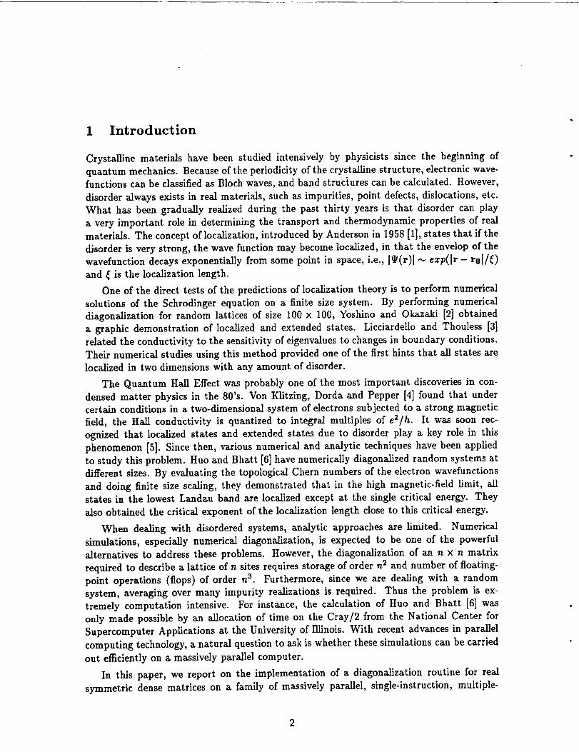
1 Introduction

Crystalline materials have been studied intensively by physicists since the beginning of

quantum mechanics. Because of the periodicity of the crystalline structure, electronic wave-functions can be classified as Bloch waves, and band structures can be calculated. However,

disorder always exists in real materials, such as impurities, point defects, dislocations, etc.

What has been gradually realized during the past thirty years is that disorder can play

a very important role in determining the transport and thermodynamic properties of real

materials. The concept of localization, introduced by Anderson in 1958 [1], states that if the

disorder is very strong, the wave function may become localized, in that the envelop of the

wavefunction decays exponentially from some point in space, i.e., [_(r)[ ,,_ exp(tr- r0[/_)

and _ is the localization length.

One of the direct tests of the predictions of localization theory is to perform numerical

solutions of the Schrodinger equation on a finite size system. By performing numerical

diagonalization for random lattices of size 100 × 100, Yoshino and Okazaki [2] obtained

a graphic demonstration of localized and extended states. Licciardello and Thouless [3]

related the conductivity to the sensitivity of eigenvalues to changes in boundary conditions.

Their numerical studies using this method provided one of the first hints that all states are

localized in two dimensions with any amount of disorder.

The Quantum HaLl Effect was probably one of the most important discoveries in con-

densed matter physics in the 80's. Von Klitzing, Dorda and Pepper [4] found that under

certain conditions in a two-dimensional system of electrons subjected to a strong magnetic

field, the Hall conductivity is quantized to integral multiples of e2/h. It was soon rec-

ognized that localized states and extended states due to disorder play a key role in this

phenomenon [5]. Since then, various numerical and analytic techniques have been applied

to study this problem. Huo and Bhatt [6] have numerically diagonalized random systems at

different sizes. By evaluating the topological Chern numbers of the electron wavefunctions

and doing finite size scaling, they demonstrated that in the high magnetic-field limit, allstates in the lowest Landau band are localized except at the single critical energy. They

also obtained the critical exponent of the localization length close to this critical energy.

When dealing with disordered systems, analytic approaches are limited. Numerical

simulations, especially numerical diagonalization, is expected to be one of the powerful

alternatives to address these problems. However, the diagonalization of an n × n matrix

required to describe a lattice of n sites requires storage of order n 2 and number of floating-

point operations (flops) of order n 3. Furthermore, since we are dealing with a random

system, averaging over many impurity realizations is required. Thus the problem is ex-

tremely computation intensive. For instance, the calculation of Huo and Bhatt [6] was

only made possible by an allocation of time on the Cray/2 from the National Center for

Supercomputer Applications at the University of Illinois. With recent advances in parallel

computing technology, a natural question to ask is whether these simulations can be carried

out efficiently on a massively parallel computer.

In this paper, we report on the implementation of a diagonalization routine for real

symmetric dense matrices on a family of massively parallel, single-instruction, multiple-

data (SIMD) computers, the Maspar MP-1 and MP-2. We find that a modification of the

standard serial algorithm can be implemented efficiently on such a highly parallel SIMD

machine. Moreover, despite the relatively low-level language, and a distributed memory, the

software can be implemented easily because of a distributed-object-oriented programming

style provided by the Maspar Linear Algebra Building Block (MPLABB) library.

This paper is organized as follows. Section II is an introduction to the MP-1 architecture.

Section III describes the algorithm and its implementation. Section IV presents numerical

results and timing data. The paper concludes with a discussion in Section V.

2 The Maspar MP-x Systems

The MP-1 and MP-2 architectures consist of the following tWO subsystems:

• The Array Control Unit (ACU)

• The Processing Element (PE) Array

The ACU is a 32-bit, custom integer RISC that stores the program, the instruction fetching

and decoding logic, and is used for scalars, loop counters and the like. It includes its own

private memory.

The PE array is a two-dimensional mesh of processors. Each processor may communicate

directly with its 8 nearest neighbors. The processors at the edges of the mesh are connected

by wrap-around channels to those at the opposite edge, making the array a two-dimensionaltorus. The two directions in the PE array are referred to as the x and y axes of the machine.

The machine dimensions are referred to as nxproc and nyproc, and the number of processors

is nproc - nyproc, nxproc. Thus, every PE has an x coordinate ixproc and a y coordinate

iyproc, and also a serial number iproc -- ixproc + nxproc . iyproc.

Each PE in the array is a RISC processor with 64K bytes of local memory. All PEs

execute the same instruction, broadcast by the ACU. The machine clock rate is 12.5 MHz.

The set of all PE memories is called parallel memory or PMEM; it is the main data

memory of the machine. Ordinarily, PMEM addresses are included in the instruction, sothat all PEs address the same element of their local memory. By a memory layer we mean

the set of locations at one PMEM address, but across the whole array of PEs. Each PE

also includes 16 64-bit registers.

The hardware supports three communication primitives:

• ACU-PE communication;

• Nearest neighbor communications among the PEs;

• Communication in arbitrary patterns through a hardware global router.

These actions are expressed in the instruction set as synchronous, register-to-register op-

erations. This allows interprocessor communication with essentially zero latency and very

high bandwidth -- 200 Gbits per second for nearest neighbor communication, for example.

3

On the MP-1, hardware arithmetic occurs on 4-bit data. Instructions that operate

on 8, 16, 32, and 64-bit integers and on 32 and 64-bit IEEE floating-point numbers are

implemented in microcode. All operations occur on data in registers; only load and storeinstructions reference memory. Peak performance of a full 16K MP-1 is 550 Mflops on

IEEE 64-bit floating-point data. The MP-2 uses 32-bit hardware integer arithmetic, with

microcode for higher precision and floating-point operations. Peak performance goes up to

nearly 2000 Mflops in the MP-2.

Because floating-point arithmetic is implemented in microcode, it is slow relative to

memory reference or interprocessor communication; these take less time than a multipli-

cation. Thus, communication and memory traffic, traditional causes of low performance

(relative to peak performance) on parallel machines, are not a serious obstacle here.

3 Algorithm and Implementation

The now standard serial algorithm [7] for computing the eigenvalues and eigenvectors of a

real symmetric matrix consists of three phases:

o

o

Reduction of the real symmetric matrix A to tridiagonal form via orthogonal simi-

larity transformations (QTAQ = T where Q is orthogonal and T is real, symmetric,

tridiagonal).

QR iteration to find all the eigenvalues and eigenvectors of the tridiagonal matrix T,or bisection and inverse iteration if only few of the eigenvalues and(or) eigenvectors are

needed (VTTV = A, where V has k orthonormal columns and A = diag(A1,..., _k)

holds the desired eigenvalues).

3. Matrix multiplication to recover the eigenvectors of A (the columns of U = QV).

3.1 Algorithms for the Parallel Computation of Eigensystems

Parallel implementation of the QR iteration phase has proved to be quite difficult. For this

reason, the Jacobi method for the symmetric eigenproblem has attracted much attention,because it is inherently parallel [8]. Unfortunately, the number of floating point operations

required by the Jacobi method is much greater than the number required by methods based

on tridiagonalization.

On many recent high-performance computers, both memory reference and interprocessorcommunication are much slower than arithmetic. This has led to the development and use

of families of algorithms that exhibit locality of reference to data, as these algorithms make

fewer memory and off-processor references per operaiion. For matrix computations, block

algorithms, which break the computation down into tasks that operate on submatrices, have

been very successful for these reasons. One advantage of the Jacobi method is that there

are good block variants of this type [9, 10], while block tridiagonalization methods are less

satisfactory. For these reasons, we first attempted an implementation of a variant of the

standardalgorithm. Since this implementation achieves high efficiency, we did not consider

implementation of a Jacobi algorithm.

For the symmetric tridiagonal eigenvalue problem, both Cuppen's divide-and-conquer

method [12] and bisection followed by inverse iteration have been advocated for the shared

memory, multiprocessor environment [13]. While both methods provide both the eigenvalues

and eigenvectors of the tridiagonal matrix, in both cases some subsequent orthogonalization

step is needed for the eigenvectors corresponding to very close eigenvalues.

In an SIMD machine each processor executes exactly the same command at each cycle.

Bisection and inverse iteration are well suited to the SIMD discipline, while the divide and

conquer method appears to be less so. Also, at the time of our work, the accuracy of the

divide and conquer method and means for its reliable implementation were still the subject

of ongoing research [12]. We therefore chose bisection.

3.2 MPL Programming on the Maspar

Our code is written in the language MPL, a data-parallel variant of C provided by Maspar.

In MPL, variables have a storage class, either singular or plural. Singular variables aretraditional C variables of any type. On the other hand, if x is declared via plural double

x, then there is an instance of x on every PE, so that x is implicitly an array. The operation

x *ffi 2; causes every PE to multiply its x by 2; this is the only way to express parallelism

in MPL.

The integer constants nxproc, nyproc, and nproc (which define the machine size) are

predefined in MPL, as are the plural integer constants iyproc, ixproc, and iproc (which

define processor coordinates).

Since matrix and vector data structures may involve more than nproc elements, several

memory locations on each processor, organized as a plural array, are required for their

storage. The MPL programmer must code the loops over these arrays required to implement

simple matrix and vector operations such as the addition of two vectors. This process, akin

to strip mining in vector machines with limited-length vector instructions (Cray machines,

for example) is usually called virtualization; it is required to create a programming model in

which there is one virtual processor per matrix or vector element. Since MPL (unlike Maspar

Fortran, Fortran 90, or the C" language developed by Thinking Machines Corporation) is

not a virtual language, the MPL programmer ordinarily virtualizes by hand.

To simplify the coding of matrix and vector operations, Maspar provides a library (the

MPLABB library) of simple operations on matrices and vectors of arbitrary size. The vir-

tualization looping is hidden within this software layer. The types of data object supported

are

• Vex. A one-dimensional array whose ith element resides in processor (i mod nproc).

In a vex u, the x coordinate of the processor holding u(i) varies most rapidly as i

increases. If the vector length is greater than nproc, multiple memory layers are used

for its storage. If its length is n, then nb = (n+ nproc - 1) + nproc layers are declared

(plural double u[nb]); element i is stored in memory layer i + nproc.

5

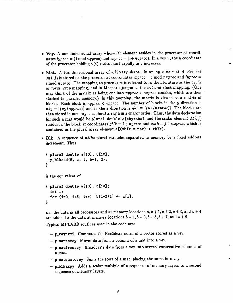
• Vey. A one-dimensionalarray whose ithelement residesin the processorat coordi-

natesiyproc= (imod nyproc) and izproc= (i-nyproc). In a vey u,the y coordinate

ofthe processorholdingu(i)variesmost rapidlyas i increases.

• Mat. A two-dimensional array of arbitrary shape. In an ny × nz mat A, element

A(i, j) is stored on the processor at coordinates izproc = j mod nzproc and iyproc =

i mod nyproc. The mapping to processors is referred to in the literature as the cyclic

or torus wrap mapping, and in Maspax's jargon as the cut and stack mapping. (One

may think of the matrix as being cut into nyproc × nzproc cookies, which axe then

stacked in parallel memory.) In this mapping, the matrix is viewed as a matrix of

blocks. Each block is nyproc × nzproc. The number of blocks in the y direction is

nby = [(ny/nyproc)] and in the x direction is nbz = [(nz/nzproc)]. The blocks are

then stored in memory as a plural array a in z-major order. Thus, the data declaration

for such a mat would be plural double a[nby*nbx], and the scalar element A(i,j)

resides in the block at coordinates yblk = i + nyproc and zblk = j + nzproc, which is

contained in the plural array element al'(yblk * nbx) + xblk].

• Blk. A sequence of nblks plural variables separated in memory by a fixed address

increment. Thus

{ plural double a[10], b[10] ;

p_blkadd(5, a, 1, b+l, 2);

)

isthe equivalentof

{ plural double a[10], b[10] ;

int i;

for (i-0; i<5; i++) b[l+2*i] += a[i];

}

i.e. the data in all processors and at memory locations a, a + 1, a + 2, a + 3, and a + 4

axe added to the data at memory locations b+ 1,b+ 3, b+ 5,b+ 7, and b+ 9.

Typical MPLABB routines used in the code axe:

- p_veynrm2 Computes the Euclidean norm of a vector stored as a vey.

- p.mattowy Moves data from a column of a mat into a vey.

- p_matfromvey Broadcasts data from a vey into several consecutive columns ofa mat.

- p_matsumtowy Sums the rows of a mat, placing the sums in a vey.

- p_blkaxpy Adds a scalar multiple of a sequence of memory layers to a second

sequence of memory layers.

3.3 Implementation

In this sectionwepresent a straightforward implementation of a parallel method based on

tridiagonalization on the MP-x computers. Our codes can perform the following functions:

• Householder reduction of a real symmetric matrix to a tridiagonal matrix.

• Finding the eigenvalues and optionally the eigenvectors of a real symmetric tridiagonal

matrix.

• Finding the eigenvalues and optionxlly the eigenvectors of a real symmetric matrix.

All eigenvalues, or those in an interval of the real axis, or all the eigenvalues from the ith

to the jth largest can be computed.

The eigenvalues and eigenvectors of the tridiagonal matrix T are computed by an embar-

rassingly parallel algorithm employing bisection and inverse iteration methods. Bisection

allows the computation of the jth largest eigenvalue. Conceptually, processor j uses bisec-

tion to find the jth eigenvalue, in parallel with all the other processors. Having found its

eigenvaJue, processor j then uses inverse iteration to find the corresponding eigenvector, if

needed. Orthogonalization of the computed eigenvectors [15] is then performed as needed.

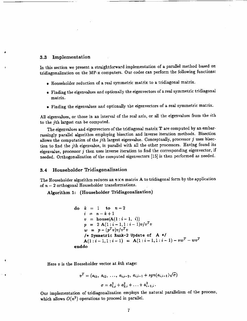
3.4 Householder Tridiagonalization

The Householder algorithm reduces an n x n matrix A to tridiagonal form by the appUcation

of n - 2 orthogonal Householder transformations.

Algorithm 1: (Householder Tridiagonalization)

do k = i to n- 2

i = n-k+l

v = house(A(l:i- 1, i))

p = 2 A(1 : i - 1, 1 : i - 1)v/vTv

w = p- (pTv)v/vTv

/, Symmetric Rank-2 Update of A */

A(1:i-1,1:i-1) = A(l:i-l,l:i-1)-vw T-wv T

enddo

Here v is the Householder vector at kth stage:

V T = (all, ai2, ..., ai,i-2, ai,i-1 + sgn(ai,i-1)V/_)

G = a 2 a 2 a 21,i nu 2,i "_''''+ i-l,i"

Our implementation of tridiagonalization employs the natural parallelism of the process,

which allows O(n 2) operations to proceed in parallel.

TheHouseholder reduction starts in the n th column of A, not the first. For a sequential

machine, this does not make any difference. On the Maspar, however, this reduces the

communication cost significantly. The reason is that at any stage k, A is tridiagonal in its

last k - 1 rows and columns, and we only need to update the ,first n - k rows and columns,which can be viewed as a submatrix with no offset.

The implementation is based on MPLABB routines. Matrices are stored as mats. Vec-tors as vexes and veys. At the ith step, the elements A(1 : i- 1, i) are extracted and

placed in a vey using p._attovey. Computation of a uses the routine p_vaynrm2. The

vector p is computed by a matrix-vector product routine that in turn uses p_blkaxpy and

p_matsmntovey. Finally, the rank-2 update of A uses pAnatfromvey, p._atfromvex, and

p_blkaxpy. Use of the MPLABB reduced the time required to develop our codes by a

significant factor.

To reduce the communication overhead, array type conversions, e.g., conversion of a

vector from vex form to vey form, have been minimized.

3.5 Bisection

The bisection procedure recursively halves an initial interval containing all eigenvalues (de-

termined from the Gershgorin circle theorem). In our implementation of bisection, processor

iproc computes eigenvaiues indexed iproc, nproc+ iproc, etc. A Sturm sequence is evaluated

by a simple, stable, first-order recurrence to determine the number of eigenvalues less than

or equal to the interval's midpoint. The half-intervai containing the desired eigenvalue is

then selected.

Each processor stores only the two boundary values of an interval containing the eigen-

value for which it is searching. To save memory, the diagonal and off-diagonal elements of

the tridiagonal matrix are broadcast at each step.

If n < ,proc then load-balance is poor, since only processors 0,..., n - 1 have anything

to do. The cost of the bisection phase, however, is quite modest, so we don't view this

as a real problem. An alternative scheme, which we have not implemented, would use

p - [nproc/nJ processors per eigenvaiue when n < nproc. The processors could subdivide

the containing interval into p -t- 1 equal subintervals, evaluate the Sturm sequence at the p

internal breakpoints simultaneously, and thereby contract the interval by a factor of p.

We have, in fact, now implemented a form of this idea. Initially, all the eigenvalues liein one interval. We subdivide it into nproc + 1 subintervals with nproc internal, equally

spaced points x_, 1 < i < nproc. Processors i then computes a Sturm sequence at x_ todetermine the number v_ of eigenvalues to the left. Then, by communicating with processor

i - 1, processor i computes vi - vi-1, which is the number of eigenvalues in the interval

(xi-1, xi]. We then switch to the parallel bisection process above, with each processor now

beginning with one of these smaller intervals. This first step, with one parallel evaluation of

a Sturm sequence, reduces all the intervals by the factor nproc; it therefore saves log 2 nproc

subsequent steps. This reduced running time by roughly 20% on full 214 processor machines.

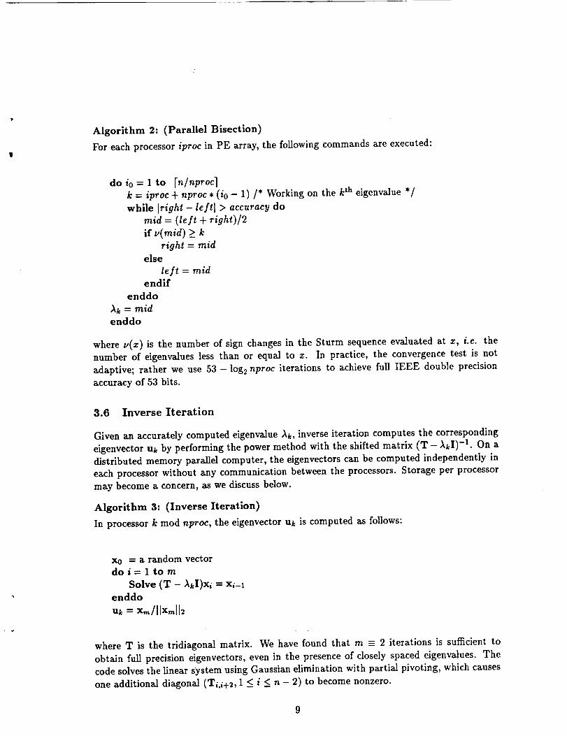
Algorithm 2: (Parallel Bisection)

For each processor iproc in PE array, the following commands are executed:

do i0 = 1 to [n/nproc]

k = iproc q- nproc * (io - 1)/* Working on the k th eigenvalue */

while Iright - leftl > accuracy do

raid = (left + right)/2

if v(mid) > k

right = mid

else

left = raidendif

enddo

)_k = midenddo

where v(x) is the number of sign changes in the Sturm sequence evaluated at z, i.e. the

number of eigenvalues less than or equal to z. In practice, the convergence test is not

adaptive; rather we use 53- log 2 nproc iterations to achieve full IEEE double precision

accuracy of 53 bits.

3.6 Inverse Iteration

Given an accurately computed eigenvalue )_k, inverse iteration computes the corresponding

eigenvector uk by performing the power method with the shifted matrix (T - )_kI) -1. On a

distributed memory parallel computer, the eigenvectors can be computed independently in

each processor without any communication between the processors. Storage per processor

may become a concern, as we discuss below.

Algorithm 3: (Inverse Iteration)

In processor k mod nproc, the eigenvector uk is computed as follows:

x0 - a random vectordo i - 1 to ra

Solve (T - RkI)xi = xi-_enddo

uk- Xm/llXmll

where T is the tridiagonal matrix. We have found that ra = 2 iterations is su_cient to

obtain full precision eigenvectors, even in the presence of closely spaced eigenvalues. The

code solves the linear system using Gaussian elimination with partial pivoting, which causes

one additional diagonal (Ti,i+2, 1 < i < n - 2) to become nonzero.

9

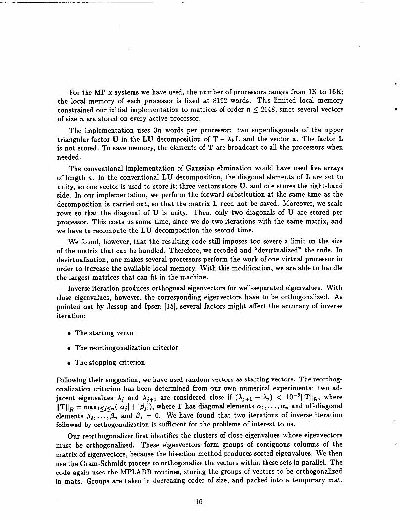
For the MP-x systems we have used, the number of processors ranges from 1K to 16K;

the local memory of each processor is fixed at 8192 words. This limited local memory

constrained our initial implementation to matrices of order n _< 2048, since several vectors

of size n are stored on every active processor.

The implementation uses 3n words per processor: two superdiagonals of the upper

triangular factor U in the LU decomposition of T - ),kI, and the vector x. The factor Lis not stored. To save memory, the elements of T are broadcast to all the processors when

needed.

The conventional implementation of Gaussian elimination would have used five arrays

of length n. In the conventional LU decomposition, the diagonal elements of L are set to

unity, so one vector is used to store it; three vectors store U, and one stores the right-hand

side. In our implementation, we perform the forward substitution at the same time as the

decomposition is carried out, so that the matrix L need not be saved. Moreover, we scale

rows so that the diagonal of U is unity. Then, only two diagonals of U are stored per

processor. This costs us some time, since we do two iterations with the same matrix, and

we have to recompute the LU decomposition the second time.

We found, however, that the resulting code still imposes too severe a limit on the sizeof the matrix that can be handled. Therefore, we recoded and "devirtuallzed" the code. In

devirtualization, one makes several processors perform the work of one virtual processor in

order to increase the available local memory. With this modification, we are able to handle

the largest matrices that can fit in the machine.

Inverse iteration produces orthogonal eigenvectors for well-separated eigenvalues. With

close eigenvalues, however, the corresponding eigenvectors have to be orthogonalized. As

pointed out by Jessup and Ipsen [15], several factors might affect the accuracy of inverseiteration:

• The starting vector

• The reorthogonalization criterion

• The stopping criterion

Following their suggestion, we have used random vectors as starting vectors. The reorthog-onalization criterion has been determined from our own numerical experiments: two ad-

jacent eigenvalues Aj and Aj+I are considered close if (Aj+I - Aj) < 10-SIlT[JR, where

]]Tlln = maxl<i<n(lajl + ]/_j]), where T has diagonal elements al,...,an and off-diagonal

elements /3_,...,fin and /31= 0. We have found that two iterations of inverse iteration

followed by orthogonalization is sufficient for the problems of interest to us.

Our reorthogonalizer first identifies the clusters of close eigenvalues whose eigenvectors

must be orthogonalized. These eigenvectors form groups of contiguous columns of the

matrix of eigenvectors, because the bisection method produces sorted eigenvalues. We then

use the Gram-Schmidt process to orthogonalize the vectors within these sets in parallel. The

code again uses the MPLABB routines, storing the groups of vectors to be orthogonalized

in mats. Groups are taken in decreasing order of size, and packed into a temporary mat,

10

until the number of columns reaches nxproc. The code then performs the Gram-Schmidt

process, working on several groups in parallel and on all columns within a group in parallel.

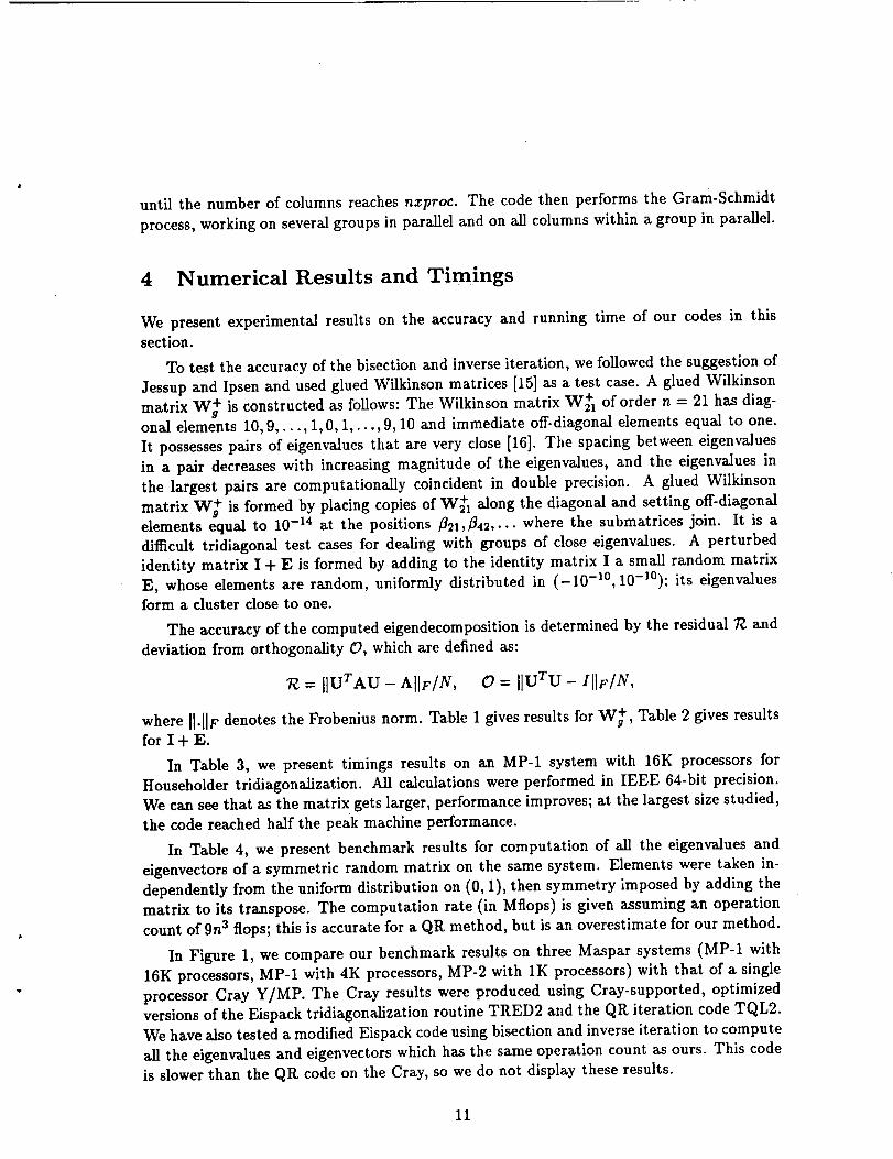
4 Numerical Results and Timings

We present experimental results on the accuracy and running time of our codes in this

section.

To test the accuracy of the bisection and inverse iteration, we followed the suggestion of

Jessup and Ipsen and used glued Wilkinson matrices [15] as a test case. A glued Wilkinson

matrix W + is constructed as follows: The Wilkinson matrix W+I of order n = 21 has diag-onal elements 10, 9,..., 1, 0, 1,..., 9, 10 and immediate off-diagonal elements equal to one.

It possesses pairs of eigenvalues that are very close [16]. The spacing between eigenvalues

in a pair decreases with increasing magnitude of the eigenvalues, and the eigenvalues in

the largest pairs are computationally coincident in double precision. A glued Wilkinson

matrix W + is formed by placing copies of W+I along the diagonal and setting off-diagonalelements equal to 10-14 at the positions _21,_42,... where the submatrices join. It is a

difficult tridiagonal test cases for dealing with groups of close eigenvalues. A perturbed

identity matrix I + E is formed by adding to the identity matrix I a small random matrix

E, whose elements are random, uniformly distributed in (-10 -1°, 10-1°); its eigenvaiues

form a cluster close to one.

The accuracy of the computed eigendecomposition is determined by the residual 7_ and

deviation from orthogonality O, which are defined as:

= IIUTAU - AHF/N, O = IIUTU- I[IF/N,

where II.lIFdenotes the Frobenius norm. Table 1 gives results for W_, Table 2 gives results

for I+ E.

In Table 3, we present timings results on an MP-1 system with 16K processors for

Householder tridiagonalization. All calculations were performed in IEEE 64-bit precision.

We can see that as the matrix gets larger, performance improves; at the largest size studied,

the code reached half the peak machine performance.

In Table 4, we present benchmark results for computation of all the eigenvalues and

eigenvectors of a symmetric random matrix on the same system. Elements were taken in-

dependently from the uniform distribution on (0, 1), then symmetry imposed by adding the

matrix to its transpose. The computation rate (in Mflops) is given assuming an operation

count of 9n a flops; this is accurate for a QR method, but is an overestimate for our method.

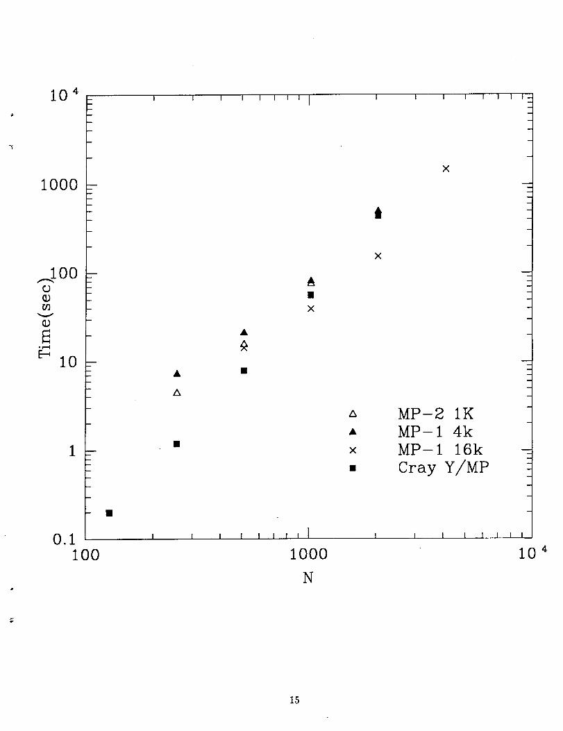
In Figure 1, we compare our benchmark results on three Maspax systems (MP-1 with

16K processors, MP-1 with 4K processors, MP-2 with 1K processors) with that of a single

processor Cray Y/MP. The Cray results were produced using Cray-supported, optimized

versions of the Eispack tridiagonalization routine TRED2 and the QR iteration code TQL2.

We have also tested a modified Eispack code using bisection and inverse iteration to compute

all the eigenvalues and eigenvectors which has the same operation count as ours. This code

is slower than the QR code on the Cray, so we do not display these results.

11

5 Conclusion

In this paper, we have described an implementation of matrix diagonalization on a massively

parallel SIMD computer. We have demonstrated that massively parallel SIMD machines are

very suitable for this kind of problem. Reliable, efficient, well-understood algorithms workwell on these machines, which is a bit of a surprise. Also, despite the necessity of working

with relatively low-level parallel programming tools, we were able to develop efficient codes

readily through the use of a software layer for operation on distributed arrays. We expect

that this approach will work well for many problems involving dense matrices and arrays.

6 Acknowledgements

Yah Huo acknowledges support from Electrical Engineering Department, Princeton Uni-

versity. Work at Princeton was performed under DEC DPRI grant and NSF CISE instru-

mentation grant CDA-9121709. He would also like to thank MasPar Computer Corp. for

their hospitality during his visit. Robert Schreiber's work was supported by NASA under

Contract NAS 2-13721 with the Universities Space Research Association.

12

References

[1] Anderson, P. W. Phys. Rev. 109, 1492 (1958).

[2] Yoshino S. and Okazaki, M. J. Phys. Soc. Jpn. 43, 415 (1977).

[3] Licciardello, D. C. and Thouless, D. J. J. Phys. C 8, 4157 (1975).

[4] Von Klitzing, K., Dorda G., and M. Pepper, Phys. Rev. Lett. 45, 494 (1980). For a

review, see Prange R. E. and Girvin, S. M. 1990, The Quantum Hall Effect. Springer-

Verlag.

[5] Halperin, B. I., Phys. Rev. B 25, 2185 (1982).

[6] Huo, Y. and Bhatt, R. N. Phys. Rev. Lett. 68, 1375 (1992).

[7] Wilkinson, J. H., and Reinsch, C. 1971, Linear Algebra, vol. II of Handbook .for Auto-

matic Computation. New York: Springer-Verlag.

[8] Golub, G. H., and Van Loan, C. F., Matrix Computation. The Johns Hopkins University

Press, second edition, 1989.

[9] Scott, D. S., Heath, M. T., and Ward, R. C., Lin. Alg. and Its Applic. 77, 345(1986).

[10] Shroff, G. and Schreiber, R., SIAM J. Matrix Anal. and Applics. 10 (1989).

[11] Maspar Mathematics Library (MPML) Reference Manual.

[12] Dongarra, J. J. and Sorensen D. C., SIAM J. Sci. Star. Comput. 8, 139(1987).

[13] Ipsen, I. C. F., and Jessup, E. R., SIAM J. Sci. Star. Comput. 11,203(1990).

[14] see, for example, TINVIT in EISPACK.

[15] Jessup, E. R., and Ipsen, I. C. F., SIAM J. Sci. Star. Comput. 13, 550(1992).

[16] Wilkinson, J. The Algebraic Eigenvalue Problem, Clarendon Press, Oxford, U.K., 1965.

13

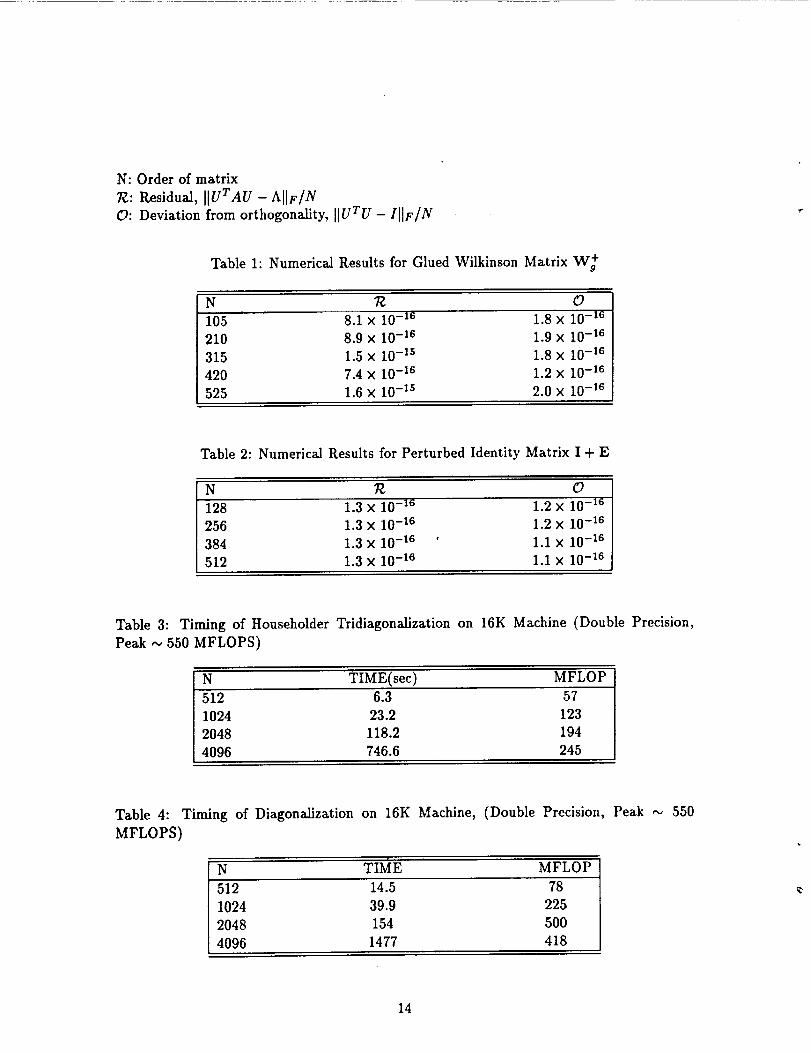
N: Order of matrix

T_: Residual, HUT AU -A[IF/N

O: Deviation from orthogonality, []uTu - II[F/N

Table 1: Numerical Results for Glued Wilkinson Matrix W +

N T¢ 0

105 8.1X I0 -16 1.8x 10-16

210 8.9x 10-16 1.9x 10-16

315 1.5x 10-15 1.8x 10-16

420 7.4x 10-16 1.2x 10-16

525 1.6x I0-Is 2.0x 10-16

Table 2: Numerical Results for Perturbed Identity Matrix I + E

N R O

128 1.3x 10-16 1.2x 10-16

256 1.3x 10-16 1.2× 10 -16

384 1.3x 10-16 • 1.1x 10-16

512 1.3x 10-16 I.Ix 10-16

Table 3: Timing of Householder Tridiagonalization on 16K Machine (Double Precision,

Peak ,,, 550 MFLOPS)

N TIME(sec) MFLOP

512 6.3 57

1024 23.2 123

2048 118.2 194

4096 746.6 245

Table 4: Timing of Diagonalization on 16K Machine, (Double Precision, Peak ,,, 550

MFLOPS)

N TIME MFLOP

512 14.5 78

1024 39.9 225

2048 154 500

4096 1477 418

14

i000

0

GQ

-m--I

E-.10

i

0.i

A

I00

I I I I I

X

I I I I ]

i000

N

/k

X

i

X

I I I

X

MP-2 IKMP-I 4k

MP-I 16k

Cray Y/MP

I I I

I I I I-

I I I I

10 4

15