Validation of Wind Power Plant Modeling Approaches in

NREL is a national laboratory of the U.S. Department of Energy Office of Energy Efficiency & Renewable Energy Operated by the Alliance for Sustainable Energy, LLC This report is available at no cost from the National Renewable Energy Laboratory (NREL) at www.nrel.gov/publications.

Contract No. DE-AC36-08GO28308

Conference Paper NREL/CP-5000-72706 May 2019

Validation of Wind Power Plant Modeling Approaches in Complex Terrain

Preprint Eliot Quon, Paula Doubrawa, Jennifer Annoni, Nicholas Hamilton, and Matthew Churchfield

National Renewable Energy Laboratory

Presented at the American Institute of Aeronautics and Astronautics SciTech Forum San Diego, California January 7–11, 2019

NREL is a national laboratory of the U.S. Department of Energy Office of Energy Efficiency & Renewable Energy Operated by the Alliance for Sustainable Energy, LLC This report is available at no cost from the National Renewable Energy Laboratory (NREL) at www.nrel.gov/publications.

Contract No. DE-AC36-08GO28308

National Renewable Energy Laboratory 15013 Denver West Parkway Golden, CO 80401 303-275-3000 • www.nrel.gov

Conference Paper NREL/CP-5000-72706 May 2019

Validation of Wind Power Plant Modeling Approaches in Complex Terrain

Preprint Eliot Quon, Paula Doubrawa, Jennifer Annoni, Nicholas Hamilton, and Matthew Churchfield

National Renewable Energy Laboratory

Suggested Citation Quon, Eliot, Paula Doubrawa, Jennifer Annoni, Nicholas Hamilton, and Matthew Churchfield. 2019. Validation of Wind Power Plant Modeling Approaches in Complex Terrain: Preprint. Golden, CO: National Renewable Energy Laboratory. NREL/CP-5000-72706. https://www.nrel.gov/docs/fy19osti/72706.pdf.

https://www.nrel.gov/docs/fy19osti/72706.pdf

NOTICE

This work was authored by the National Renewable Energy Laboratory, operated by Alliance for Sustainable Energy, LLC, for the U.S. Department of Energy (DOE) under Contract No. DE-AC36-08GO28308. Funding provided by the U.S. Department of Energy Office of Energy Efficiency and Renewable Energy Wind Energy Technologies Office. The views expressed herein do not necessarily represent the views of the DOE or the U.S. Government. The U.S. Government retains and the publisher, by accepting the article for publication, acknowledges that the U.S. Government retains a nonexclusive, paid-up, irrevocable, worldwide license to publish or reproduce the published form of this work, or allow others to do so, for U.S. Government purposes.

This report is available at no cost from the National Renewable Energy Laboratory (NREL) at www.nrel.gov/publications.

U.S. Department of Energy (DOE) reports produced after 1991 and a growing number of pre-1991 documents are available free via www.OSTI.gov.

Cover Photos by Dennis Schroeder: (clockwise, left to right) NREL 51934, NREL 45897, NREL 42160, NREL 45891, NREL 48097, NREL 46526.

NREL prints on paper that contains recycled content.

http://www.nrel.gov/publications

http://www.osti.gov/

Validation of Wind Power Plant Modeling Approaches

in Complex Terrain

Eliot Quon, Paula Doubrawa, Jennifer Annoni, Nicholas Hamilton, and Matthew Churchfield

National Renewable Energy Laboratory, Golden, Colorado, 80401, USA

The effect of terrain on wind-power-plant aerodynamics is often neglected due to thecomplexity of terrain-atmosphere-turbine interactions and the computational effort re-quired to adequately resolve the relevant physics. In this work, the effects of topographyon plant performance are investigated using a comprehensive set of measurements fromthe Wind Forecast Improvement Project 2 and three modeling approaches operating atdifferent levels of fidelity. A high-fidelity approach consists of large-eddy simulations ona terrain-resolving mesh to produce unsteady, heterogeneous flow that is sensitive to thelocal topography, with turbines modeled as actuator lines. In comparison, an engineeringapproach makes use of a steady-state wake model that has been modified to account forterrain effects. An intermediate level of fidelity is achieved through the use of a multi-physics model that couples wake dynamics to the aeroelastic response of each wind turbineand uses inflow from a large-eddy simulation. This paper details a case study of nine tur-bines in a near-neutral atmospheric boundary layer after a wind-speed ramp. In situ andremote-sensing measurements upstream of the wind plant are used to prescribe initial andboundary conditions to the models. Wind turbine power measurements are used to assessthe ability of the different models to capture the effects of terrain on turbine wake dynam-ics and therefore power production in an array. The study demonstrates that accountingfor unsteady turbulent inflow and averaging over time periods longer than 10 minutes arenecessary for realistic predictions of mean power output, due to unsteady, local variationsin wind speed and direction. Engineering models that account for local uphill terrainsteepness may not be sufficient in all cases as favorable pressure-gradient effects may beoverestimated and downwind terrain-induced vertical wake displacement is neglected.

I. Introduction

Wind power plants have proven to be a reliable, cost-effective source of renewable energy, and are keycomponents of the United States’ renewable energy portfolio. The U.S. Department of Energy (DOE) hasreported that 20% of the U.S. end-use demand could be satisfied by wind energy alone by 2030, and 35% by2050 [1]. To this end, modern wind plants must operate more intelligently and efficiently than before. Theperformance and efficiency of a wind plant are largely dictated by layout, wind turbine selection, controls,and atmospheric conditions. Plant layout is of importance because a power-producing wind turbine willhave a turbulent, low-speed wake that persists for some distance downstream. Therefore, the arrangement ofturbines within the plant determines the degree to which turbines can interact aerodynamically. The negativeimpact of an upstream turbine wake on downstream turbine performance may be mitigated using controls.Wake steering, for instance, uses yaw misalignment to redirect turbine wakes and minimize downstreamrotor waking [2]. The dynamics of these turbine wakes—including the extent to which they meander and thedistance at which they recover free-stream flow statistics—as well as the degree to which the wake trajectoriesmay be controlled, are modulated by atmospheric conditions. Predicting the performance of wind turbinesis further complicated by nonflat terrain, in which speedup on the windward side of hills and terrain-addedturbulence may not be reliably predicted. Neglecting terrain effects can underestimate power reduction fordownstream turbines and ultimately overestimate wind plant performance [3]. Furthermore, terrain-inducedmean or time-dependent lateral or vertical deflection of the wakes adds another layer of complexity to theconsideration of wake management and control. These challenges have motivated recent experimental andcomputational investigations [4].

1 of 18


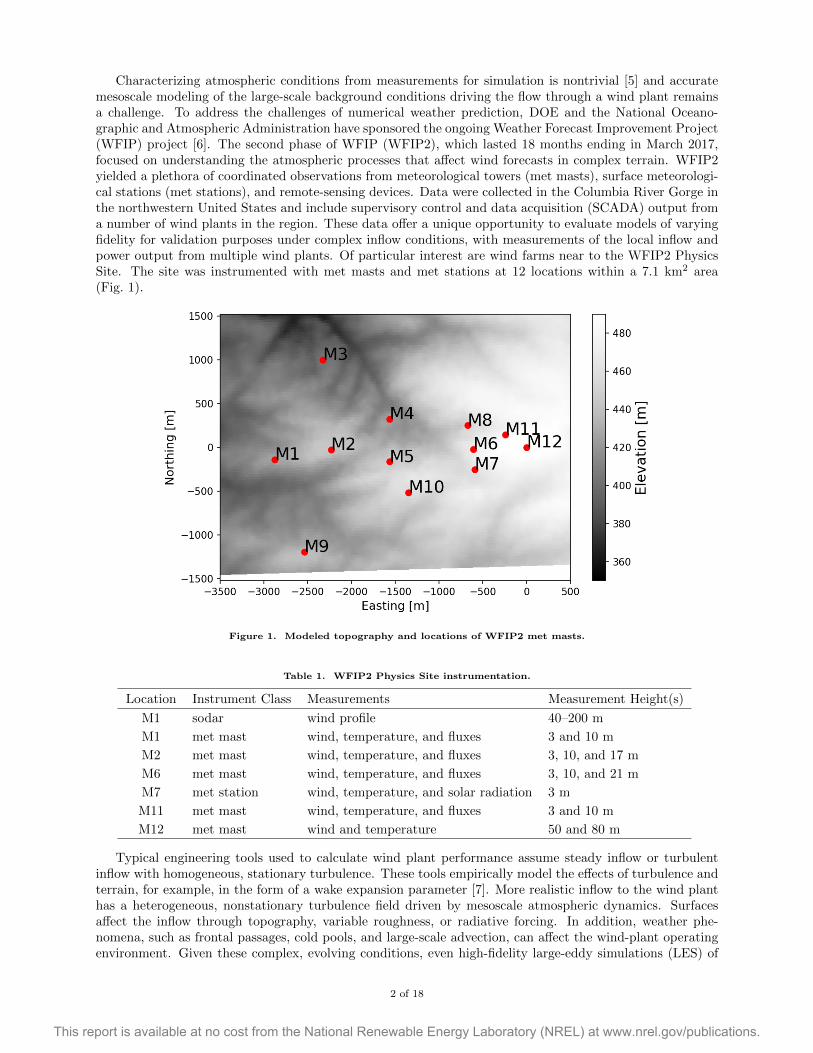
Characterizing atmospheric conditions from measurements for simulation is nontrivial [5] and accuratemesoscale modeling of the large-scale background conditions driving the flow through a wind plant remainsa challenge. To address the challenges of numerical weather prediction, DOE and the National Oceano-graphic and Atmospheric Administration have sponsored the ongoing Weather Forecast Improvement Project(WFIP) project [6]. The second phase of WFIP (WFIP2), which lasted 18 months ending in March 2017,focused on understanding the atmospheric processes that affect wind forecasts in complex terrain. WFIP2yielded a plethora of coordinated observations from meteorological towers (met masts), surface meteorologi-cal stations (met stations), and remote-sensing devices. Data were collected in the Columbia River Gorge inthe northwestern United States and include supervisory control and data acquisition (SCADA) output froma number of wind plants in the region. These data offer a unique opportunity to evaluate models of varyingfidelity for validation purposes under complex inflow conditions, with measurements of the local inflow andpower output from multiple wind plants. Of particular interest are wind farms near to the WFIP2 PhysicsSite. The site was instrumented with met masts and met stations at 12 locations within a 7.1 km2 area(Fig. 1).

Figure 1. Modeled topography and locations of WFIP2 met masts.

Table 1. WFIP2 Physics Site instrumentation.

Location Instrument Class Measurements Measurement Height(s)

M1 sodar wind profile 40–200 m

M1 met mast wind, temperature, and fluxes 3 and 10 m

M2 met mast wind, temperature, and fluxes 3, 10, and 17 m

M6 met mast wind, temperature, and fluxes 3, 10, and 21 m

M7 met station wind, temperature, and solar radiation 3 m

M11 met mast wind, temperature, and fluxes 3 and 10 m

M12 met mast wind and temperature 50 and 80 m

Typical engineering tools used to calculate wind plant performance assume steady inflow or turbulentinflow with homogeneous, stationary turbulence. These tools empirically model the effects of turbulence andterrain, for example, in the form of a wake expansion parameter [7]. More realistic inflow to the wind planthas a heterogeneous, nonstationary turbulence field driven by mesoscale atmospheric dynamics. Surfacesaffect the inflow through topography, variable roughness, or radiative forcing. In addition, weather phe-nomena, such as frontal passages, cold pools, and large-scale advection, can affect the wind-plant operatingenvironment. Given these complex, evolving conditions, even high-fidelity large-eddy simulations (LES) of

2 of 18


the atmospheric boundary layer (ABL) may neglect key physics for a given set of simulation conditions. For example, generating LES-resolved turbulence with a canonical precursor (using a strong recycling ap-proach on a separate periodic simulation domain [8]) carries the assumption that the ABL is in a stationary, quasi-equilibrium state. To simulate more realistic conditions, nonstationarity may be forced through time-varying boundary conditions and/or internal forcing terms in the governing equations [9, 10]. Most of the aforementioned sources of heterogeneity may be introduced using the boundary-condition or internal-forcing approach except for complex terrain effects.

Much of the previous high-fidelity research and analysis of wind plants in complex terrain was performed with Reynolds-averaged Navier-Stokes (RANS) solvers rather than LES [11]. However, high-fidelity LES is needed to capture turbulent motions in the ABL and accurately simulate the wind plant operating envi-ronment. A RANS study considering an idealized Gaussian hill has shown that terrain modifies the wake geometry in a nonlinear way; in other words, the wake from a turbine situated atop a hill is not the same as the superposition of flow over the hill without the turbine with the wake of a turbine on flat terrain [11]. A more recent study demonstrated that, compared to a wind-tunnel experiment, LES is able to accurately capture both the flow speedup over a Gaussian hill as well as the wake velocity deficit and added turbulence due to a turbine on top of that hill [12]. Another recent LES study highlights the computational challenges of modeling realistic complex terrain: when using a segregated pseudo-spectral flow solver, the cost to solve the pressure Poisson equation increases substantially with terrain complexity [4]. Other complex-terrain research has focused on the intricacies of LES numerical methods, including subgrid-scale modeling and the terrain representation. These modeling decisions can affect the size, shape, and location of recirculation zones on the lee side of a hill [13].

In the present study, we apply three models of increasing fidelity to evaluate the effects of complex terrain on turbines in the Columbia River Gorge, focusing on a 1-hour period following a wind speed ramp. During this 1-hour period, atmospheric conditions (described in Section II) were approximately constant. LES predictions of the heterogeneous flow field were validated against field measurements at the WFIP2 Physics Site and individual turbine power predictions from the three different models (detailed in Section III) were validated against the average power produced during the period of interest.

II. Site Characterization

The region of interest near the Columbia River Gorge and the subset of wind turbines under investigation are illustrated in Fig. 2. Locations of both the wind turbines and instrument sites are superimposed on the terrain, which were extracted from Shuttle Radar Topography Mission satellite data [14]. Table 1 summarizes the measurements from the WFIP2 Physics Site that have been used in this study.

II.A. Terrain

The current study builds on previous wind farm LES studies in flat terrain (e.g., Ref. [5, 15]). Modeling challenges in this work not only include resolving the uphill inflow and downhill outflow from the turbines, but also the flow over and around additional upwind flow features. Figures 1 and 2 identify the locations of WFIP2 measurements and turbines, respectively, and illustrate the terrain in the region. Within this study area, 25% of the terrain has a slope between 5◦ and 15◦. Figure 3(a) illustrates the terrain upwind and downwind of each of the wind turbines (WTs) in the front row (WT 1–5), whereas Fig 3(b) illustrates the terrain for the back row (WT 6–9). WT 1, for instance, is situated 0.7D above a gulch located 6D upwind, assuming westerly flow. It is important to note that reference measurements from the Physics Site were not taken from flat terrain (Fig. 3(c)). Terrain complexity, therefore, also poses challenges for the inflow validation effort. For a realistic LES turbulence field, observations from WFIP2 may correspond to simulated wind profiles that are offset from the actual measurement location due to spatial variability.

II.B. Atmospheric Conditions

Figure 4 shows observations from WFIP2 on November 21, 2016, used to characterize the wind plant inflow. This particular date is a case study from the DOE Mesoscale-to-Microscale Coupling project [16], selected based on meteorological interests that included a topographical wake from Mount Hood and mountain waves, both observed in mesoscale simulation. The reported met-mast measurements are from the 80-m tower at M12 (Fig. 1), which has four sonic anemometers: two at 50 m and two at 80 m above ground. In addition,

3 of 18


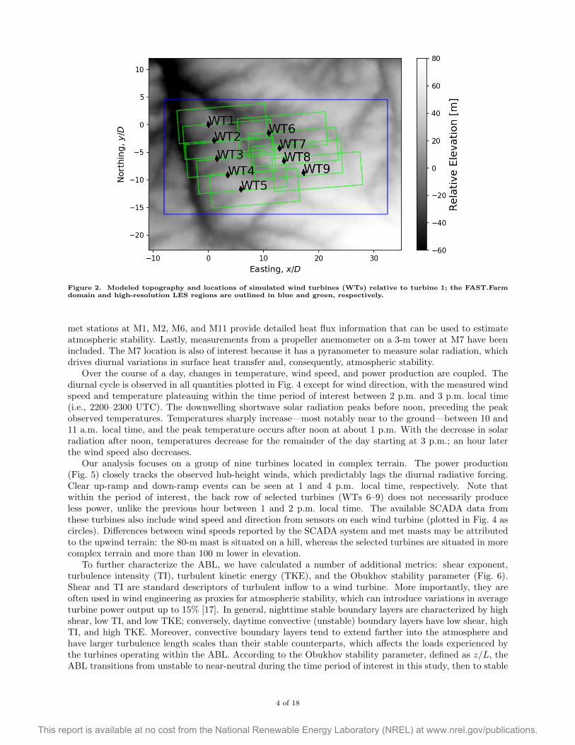
Figure 2. Modeled topography and locations of simulated wind turbines (WTs) relative to turbine 1; the FAST.Farmdomain and high-resolution LES regions are outlined in blue and green, respectively.

met stations at M1, M2, M6, and M11 provide detailed heat flux information that can be used to estimateatmospheric stability. Lastly, measurements from a propeller anemometer on a 3-m tower at M7 have beenincluded. The M7 location is also of interest because it has a pyranometer to measure solar radiation, whichdrives diurnal variations in surface heat transfer and, consequently, atmospheric stability.

Over the course of a day, changes in temperature, wind speed, and power production are coupled. Thediurnal cycle is observed in all quantities plotted in Fig. 4 except for wind direction, with the measured windspeed and temperature plateauing within the time period of interest between 2 p.m. and 3 p.m. local time(i.e., 2200–2300 UTC). The downwelling shortwave solar radiation peaks before noon, preceding the peakobserved temperatures. Temperatures sharply increase—most notably near to the ground—between 10 and11 a.m. local time, and the peak temperature occurs after noon at about 1 p.m. With the decrease in solarradiation after noon, temperatures decrease for the remainder of the day starting at 3 p.m.; an hour laterthe wind speed also decreases.

Our analysis focuses on a group of nine turbines located in complex terrain. The power production(Fig. 5) closely tracks the observed hub-height winds, which predictably lags the diurnal radiative forcing.Clear up-ramp and down-ramp events can be seen at 1 and 4 p.m. local time, respectively. Note thatwithin the period of interest, the back row of selected turbines (WTs 6–9) does not necessarily produceless power, unlike the previous hour between 1 and 2 p.m. local time. The available SCADA data fromthese turbines also include wind speed and direction from sensors on each wind turbine (plotted in Fig. 4 ascircles). Differences between wind speeds reported by the SCADA system and met masts may be attributedto the upwind terrain: the 80-m mast is situated on a hill, whereas the selected turbines are situated in morecomplex terrain and more than 100 m lower in elevation.

To further characterize the ABL, we have calculated a number of additional metrics: shear exponent,turbulence intensity (TI), turbulent kinetic energy (TKE), and the Obukhov stability parameter (Fig. 6).Shear and TI are standard descriptors of turbulent inflow to a wind turbine. More importantly, they areoften used in wind engineering as proxies for atmospheric stability, which can introduce variations in averageturbine power output up to 15% [17]. In general, nighttime stable boundary layers are characterized by highshear, low TI, and low TKE; conversely, daytime convective (unstable) boundary layers have low shear, highTI, and high TKE. Moreover, convective boundary layers tend to extend farther into the atmosphere andhave larger turbulence length scales than their stable counterparts, which affects the loads experienced bythe turbines operating within the ABL. According to the Obukhov stability parameter, defined as z/L, theABL transitions from unstable to near-neutral during the time period of interest in this study, then to stable

4 of 18


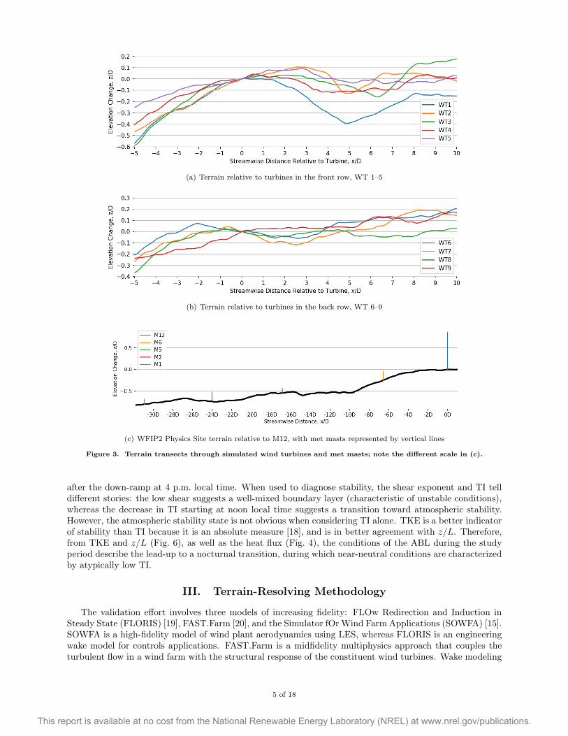
(a) Terrain relative to turbines in the front row, WT 1–5

(b) Terrain relative to turbines in the back row, WT 6–9

(c) WFIP2 Physics Site terrain relative to M12, with met masts represented by vertical lines

Figure 3. Terrain transects through simulated wind turbines and met masts; note the different scale in (c).

after the down-ramp at 4 p.m. local time. When used to diagnose stability, the shear exponent and TI telldifferent stories: the low shear suggests a well-mixed boundary layer (characteristic of unstable conditions),whereas the decrease in TI starting at noon local time suggests a transition toward atmospheric stability.However, the atmospheric stability state is not obvious when considering TI alone. TKE is a better indicatorof stability than TI because it is an absolute measure [18], and is in better agreement with z/L. Therefore,from TKE and z/L (Fig. 6), as well as the heat flux (Fig. 4), the conditions of the ABL during the studyperiod describe the lead-up to a nocturnal transition, during which near-neutral conditions are characterizedby atypically low TI.

III. Terrain-Resolving Methodology

The validation effort involves three models of increasing fidelity: FLOw Redirection and Induction inSteady State (FLORIS) [19], FAST.Farm [20], and the Simulator fOr Wind Farm Applications (SOWFA) [15].SOWFA is a high-fidelity model of wind plant aerodynamics using LES, whereas FLORIS is an engineeringwake model for controls applications. FAST.Farm is a midfidelity multiphysics approach that couples theturbulent flow in a wind farm with the structural response of the constituent wind turbines. Wake modeling

5 of 18


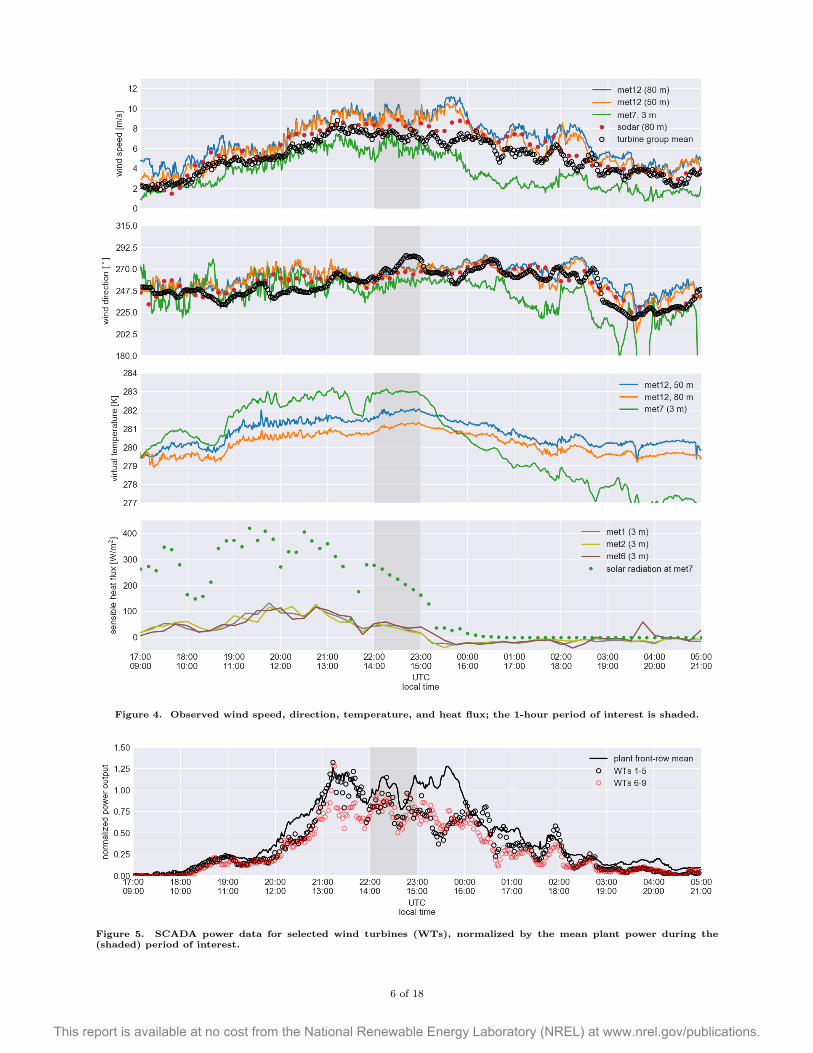
Figure 4. Observed wind speed, direction, temperature, and heat flux; the 1-hour period of interest is shaded.

Figure 5. SCADA power data for selected wind turbines (WTs), normalized by the mean plant power during the(shaded) period of interest.

6 of 18


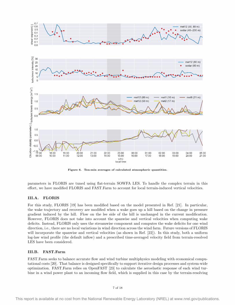
Figure 6. Ten-min averages of calculated atmospheric quantities.

parameters in FLORIS are tuned using flat-terrain SOWFA LES. To handle the complex terrain in thiseffort, we have modified FLORIS and FAST.Farm to account for local terrain-induced vertical velocities.

III.A. FLORIS

For this study, FLORIS [19] has been modified based on the model presented in Ref. [21]. In particular,the wake trajectory and recovery are modified when a wake goes up a hill based on the change in pressuregradient induced by the hill. Flow on the lee side of the hill is unchanged in the current modification.However, FLORIS does not take into account the spanwise and vertical velocities when computing wakedeficits. Instead, FLORIS only uses the streamwise component and computes the wake deficits for one winddirection, i.e., there are no local variations in wind direction across the wind farm. Future versions of FLORISwill incorporate the spanwise and vertical velocities (as shown in Ref. [22]). In this study, both a uniformlog-law wind profile (the default inflow) and a prescribed time-averaged velocity field from terrain-resolvedLES have been considered.

III.B. FAST.Farm

FAST.Farm seeks to balance accurate flow and wind turbine multiphysics modeling with economical compu-tational costs [20]. That balance is designed specifically to support iterative design processes and system-wideoptimization. FAST.Farm relies on OpenFAST [23] to calculate the aeroelastic response of each wind tur-bine in a wind power plant to an incoming flow field, which is supplied in this case by the terrain-resolving

7 of 18


SOWFA precursor simulation. For the current study, the FAST-modeled structural degrees of freedom havebeen disabled to focus on aerodynamic interactions. The aerodynamic response, based on blade-elementmomentum theory, is then used to estimate the dynamic flow field in the wake of each turbine, which isadvected downstream based on dynamic wake meandering principles. The wake flow from FAST.Farm ismoved downstream according to an effective advection velocity, calculated within a series of planes parallelto the rotor. Turbine loads are calculated in near-rotor subdomains while wake meandering and mergingcalculations are calculated on a background domain. Any point excluded from the background domain (e.g.,those points that are below the terrain surface) do not contribute to the effective advection velocity. Byinterpolating the LES field onto only points above the surface of the ground, the advection velocity is nat-urally terrain-following. The resulting turbulent wake flow does not pass through the surface, even thoughFAST.Farm does not include any explicit models for complex terrain, flow recirculation or separation, orlocal pressure gradients.

FAST.Farm simulations depend on two sampled data sets provided by a SOWFA large-eddy simulation.First, low-frequency sampling was performed every 2 s over a region encompassing all turbines of interest andextending downstream far enough so that simulated wake planes—the number of which is specified a priori—do not advect out of the sampled domain. A second, high-frequency data set was sampled concurrently at1/3-s intervals in 2D × 2D × 2D cubes centered around each turbine. This data set is used to calculateturbine power and unsteady aerodynamic loads.

III.C. SOWFA Large-Eddy Simulation

High-fidelity wake simulation is accomplished with SOWFA large-eddy simulation, which can accuratelyresolve all the energetic scales of turbulent motion in the ABL in addition to capturing the physics of wakemeandering, expansion, and recovery. The standard SOWFA simulation approach first simulates a canonicalABL on a horizontally periodic domain. Turbulent flow from this precursor LES is then mapped to a time-varying Dirichlet boundary condition on a finite-domain simulation with turbines. Turbines are modeledas actuator lines that correspond to momentum sources [15]. In this complex terrain study, we take thesame approach to turbulent inflow generation as with flat terrain. Inflow planes are extracted from the flat-terrain precursor and mapped onto the terrain-following mesh at the inlet boundary, in the same manner asRefs. [3,24]. This is a straightforward approach to generating inflow turbulence over complex terrain withouthaving to enforce periodicity. Since the inflow does not have any resolved terrain-added turbulence, the flowwill require some finite distance to adjust to the terrain. Over flat terrain, transition from under-resolvedturbulence on a 20-m grid to fully resolved turbulence on a 10-m grid can require 1–2 km [25]. In complexterrain, we expect this transition to be facilitated by topographical features.

The precursor simulation is aimed at reproducing the conditions observed in the vicinity of the turbinesat the WFIP2 Physics Site. Specifically, the high-frequency data from M12 were used to derive the mean flowconditions (from Fig. 4) and turbulence characteristics (from Fig. 6) at hub height, which were assumed tobe stationary over the 1-hour study period between 2200 and 2300 UTC. Surface roughness, an input to theSchumann-Grotzbach surface shear-stress model, was used as a tuning parameter to obtain the desired shearexponent (< 0.1) and turbulence intensity at hub height (5%–10%). At the lower surface, the measured heatflux (Fig. 4) was specified as a fixed flux boundary condition to provide heating representative of the slightlyunstable, near-neutral ABL that existed in the period prior to the nocturnal transition. Turbulence closureis achieved with the Deardorff one-equation eddy-viscosity model. The only unknowns are the temperatureprofile and consequently the ABL height. Due to limited data availability at the Physics Site, the ABLheight was estimated from the signal-to-noise ratio in measurements recorded by a radar acoustic soundingsystem located 3 miles away in Wasco, Oregon. During the study period, the temperature was assumedconstant with height, a characteristic of near-neutral conditions, through the ABL up to an estimated ABLheight of 600 m.

The precursor computational domain has uniform grid spacing of 20 m up to 1 km in height, after whichthe vertical spacing increases with height at a growth rate of 5%. The horizontal spacing is kept constantuntil the vertical spacing doubles, at which point the horizontal spacing also increases by a factor of twoto match the vertical spacing. Overall, the mesh is coarsened in this manner up to a uniform cell size of80 m and this cell size is extended up to a height of 3 km, resulting in 4.1 million computational cells.A solver-adjustable time-step size was permitted with the condition that the maximum Courant numberremains below 0.75.

In the terrain-resolving, finite-domain simulation, the mesh is refined by cell splitting to 10 m within the

8 of 18


outlined blue region in Fig. 2 to provide higher-resolution sampled fields for FLORIS and FAST.Farm. Thisapproach results in a mesh with 7.7 million computational cells. A Laplacian mesh-motion solver [26] isused to stretch the mesh over terrain mapped by the Shuttle Radar Topography Mission, with the minimumdomain height being 3 km, corresponding to the precursor domain. The redistribution of points is controlledby an inverse-distance diffusivity term. To maintain numerical stability in the flow simulation on the resultantmesh, 1/6-s time steps were simulated with a maximum Courant number of 0.3. Inflow to the lower-fidelitymodels was sampled from this simulation, ignoring the first 10 minutes of simulated time to account forterrain-induced transients.

After running the flat-terrain precursor, the simulation domain was further refined in the outlined greenregions of Fig. 2; after three refinement steps, the finest grid spacing is 1.25 m around the rotor. This cell sizeallows for over 70 cells across the rotor diameter to provide sufficient resolution for actuator line modeling.The turbine models in SOWFA and FAST.Farm are both based on manufacturer-provided aerodynamics,structural, and controls data. Overall, the final terrain- and turbine-resolving mesh contains 92 millioncomputational cells. The actuator-line simulation required a time-step size of 0.04 s that resulted in amaximum Courant number of 0.5.

IV. Results

Results from the three models are presented in the following four sections. First, we assess how wellthe LES inflow matches the observed flow (Section IV.A). Next, we validate the power predicted by thethree models against SCADA output (Section IV.B). Then, we analyze the flow field to explain our powerpredictions (Section IV.C). Finally, we characterize the different rotor wake trajectories over terrain (Sec-tion IV.D). Steady-state results from the FLORIS engineering model accounting for terrain were calculatedin minutes on a personal computer. Midfidelity FAST.Farm results were obtained with a computational costof 2 s wall clock time per second of simulation time on a 24-core high-performance-computing server. Incomparison, the high-fidelity LES required 3 minutes of wall clock time per second of simulation time whileutilizing 2064 cores (i.e., 100 core-hours per second of simulation time).

IV.A. Simulated Flow Characteristics

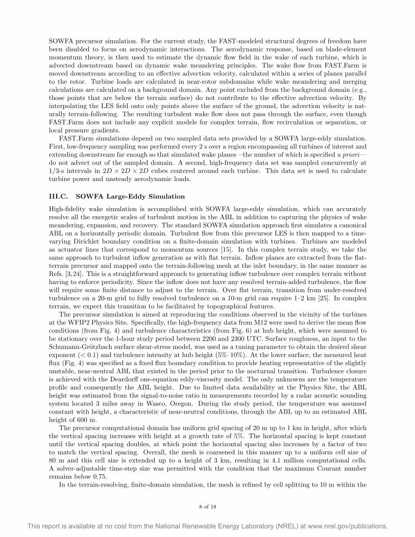
The validation against SCADA data first requires an accurate simulation of the background turbulent flow.Flow over flat terrain was simulated for 20,000 s to ensure that planar-averaged statistics are converged overtime. Figure 7 shows the simulated quantities of interest after convergence: friction velocity, wind shearexponent, TI, and TKE. Simulated quantities from the flat, horizontally periodic precursor (black curves)are compared with virtual instruments sampled within SOWFA (color curves). With the flat precursor,statistical quantities were calculated in two ways, either from planar averages (assuming homogeneity) orfrom time averages of a point probe (assuming stationarity). The latter approach replicates the treatmentof observations from the field. In all plots, the shaded region represents the range of values observed in thecorresponding real-world instruments from WFIP2.

In lieu of directly specifying a velocity profile, which is not well defined given limited height-varyingdata, the mean hub-height velocity was kept fixed and surface roughness was adjusted to match the observed

surface shear stress as described by friction velocity u∗ =[〈u′v′〉2 + 〈u′w′〉2

]0.25. Prime quantities denote

fluctuations about a mean and 〈·〉 denotes time averaging. A surface roughness of 0.005 m in SOWFA resultsin a planar-averaged u∗ that matches the measurement mean. Unlike the planar average, however, the 10-min time statistics of the flat-terrain probe displays significantly more variability. The mean u∗ is 9% lowerthan the planar average, but still within the range of observed values. Probes from the terrain-resolvingsimulation are lower than observations by 21%–34%. However, because of terrain variations, the quantitiesof interest calculated from terrain-resolved probes are not expected to match the corresponding flat-terrainvalues.

More important than matching u∗ at the ground is to match the shear across the rotor and turbulencelevel at hub height, as these quantities have a much greater impact on turbine performance and loads. Theestimated shear from the virtual sodar at M1 and virtual met mast at M12 are 0.022 and 0.032, respectively.The M12 shear closely matches the precursor value because the precursor target values were specified basedon the average values at this location. This difference may be attributed to the change in mean flow betweenM01 and M12, likely because M1 is located at 70-m lower elevation.

9 of 18


(a) Friction Velocity (at z=10 m) (b) Wind Shear

(c) Turbulence Intensity (d) Turbulent Kinetic Energy

Figure 7. Simulated conditions from the flat precursor simulation (black curves) and terrain-resolving simulation (colorcurves); the shaded region represents the range of observed values corresponding to the virtual measurements in terrain.

Turbulence levels in terms of TI and TKE are in agreement between all probe calculations, regardlessof terrain. This agreement suggests that in this case, the modest terrain variation (in terms of elevationchange and steepness) do not add an appreciable amount of turbulence and the primary terrain effect ison the mean flow. The mean and range of simulated values in both turbulence quantities is in excellentagreement with the observations at WFIP2. In addition, the velocity variances, which contribute to TI andTKE, are generally overpredicted by the planar-averaged statistics and should not be used for comparisonwith observations.

IV.B. Average Power Production

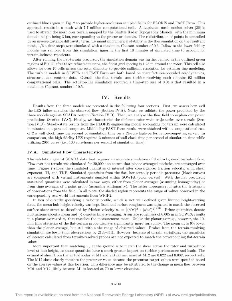
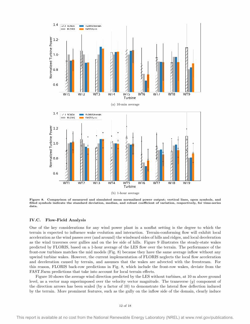
Having verified that our LES flow fields are representative of observed conditions at WFIP2 during theperiod of interest, we can now make an assessment of the power predictions for our three wind plant models.Figure 8 illustrates the mean and standard deviation (where applicable) in power for the reference SCADAdata and model outputs. Power has been normalized by the mean power from the front-row turbines, WT1–5 (Fig. 2). Because FLORIS (with and without terrain) is a steady-state model, there is no measure ofvariability available. SCADA data are available at 2-min intervals, therefore, the power statistics are basedon 30 data samples. In contrast, FAST.Farm and SOWFA have instantaneous power output at 100 Hz and25 Hz, respectively. Because we assumed that the period between 2200 and 2300 UTC is stationary, thereference SCADA data in both subplots are identical.

In total, 1.5 hours of terrain-resolved LES flow-field data (Fig. 2) are available for FLORIS and FAST.Farm.Omitting start-up transients in the LES terrain simulation retains at least 1 hour of usable inflow data, whichpermits analysis of averaging effects. However, only 9 minutes of comparable SOWFA LES turbine simula-tion time are available because of computational resource limitations, so the high-fidelity results have beenexcluded from this analysis. Figure 8 illustrates the predicted power, neglecting the initial 10 minutes ofeach turbine simulation to allow for wake development. We then compare the effects of averaging over 10

10 of 18


minutes—a standard averaging period in wind engineering practice—with a full 1-hour average to matchthe reference period. Note that the 10-min period in Fig. 8(a) overlaps with the first 10 minutes of thedata contributing to the 1-hour results in Fig. 8(b). To replicate the SCADA data processing, the 1-hourFAST.Farm data were first resampled to 2-min intervals before calculating the mean and standard deviation.Resampling of the SCADA data was not performed for the 10-min analysis, as only 5 data points wouldhave been retained and therefore precluded any statistically meaningful conclusion.

The full-hour average shows reduced variability in the FAST.Farm power output in terms of standarddeviation. However, this variability metric ranges from 15%–32% of the mean in the SCADA data, likelyresulting from data outliers and the limited sample size. As an alternative, the robust coefficient of variation(RCoV) may be considered:

RCoV =median (|P −median(P )|)

median(P )(1)

By this metric (indicated by the symbols in Fig. 8), the change in variability between turbines is negligiblefor both the SCADA and FAST.Farm data. The variability in the FAST.Farm predictions is within 11%±2%of the median, whereas the variability in measured power is within 16%±2% of the median.

Comparisons between the 10-min and 1-hour averaged power output indicate that a longer averagingperiod generally reduces the predicted change in power output resulting from terrain. In other words, theFLORIS results including terrain effects, which depend on the inflow averaging period, tend toward theflat-terrain FLORIS results (with log-law-modeled inflow) that have no time dependence. The front-rowoutput tends toward unity for the 1-hour average for both models. For the 10-min period, the mean powerfor WTs 1–5 is within 4%–15% of the front-row mean (i.e., a normalized turbine power of 1.0), and within0%–6% for the 1-hour period.

Simulated terrain effects on turbine power performance, based on Fig. 8(b), may be summarized into thefollowing terrain cases:

1. Terrain modeling may reasonably predict turbine performance in the field (WTs 2, 4, and 8).

2. Terrain modeling overpredicts turbine performance, with FLORIS and FAST.Farm in agreement (WTs1 and 3).

3. Terrain modeling underpredicts turbine performance, with FLORIS and FAST.Farm in agreement(WT5).

4. Terrain modeling underpredicts power production, with FLORIS and FAST.Farm in disagreement(WTs 6, 7, and 9).

Predictions are considered reasonable (Terrain Case 1) where the mean and/or median values are in agree-ment between the SCADA and model predictions. For Terrain Cases 1–3, FAST.Farm and FLORIS withterrain are in agreement in the front row (WTs 1–5). For all turbines in the back row (WTs 6–9), FAST.Farmand FLORIS differ significantly. Except for WT6, FLORIS with terrain results in negligible increases inpower output in the back row.

The effectiveness of the models in Terrain Case 1 is not definitive, considering that the mean and medianvalues tell different stories. Moreover, Terrain Case 1 includes a variety of terrain, as illustrated in Fig. 3: aturbine on an uphill slope (WT2), a turbine on the top of a hill (WT4), as well as a turbine on a slight downhillslope (WT8). Overpredictions of turbine performance (Terrain Case 2) typically result from overestimatingthe effect of the favorable pressure gradient. With WT2 as an exception, this trend holds true in the currentresults—WT1 and WT3 both have a relatively steep average windward slope of 13◦ (Fig. 3(a)). DespiteWT2 having a similar average windward slope of 11◦, performance is not overpredicted because the turbineis situated on the upslope rather than at a local elevation maxima.

Underpredictions in turbine performance (Terrain Cases 3 and 4) may not be directly attributed to theslope of the local terrain. With the exception of WT7, FAST.Farm turbine power predictions are in closeragreement with SCADA data than those from FLORIS (with and without terrain). This may be due to theunsteady prescribed inflow to FAST.Farm, and/or FLORIS neglecting the local flow field when advectingthe modeled turbine wakes. The terrain-induced flow physics are discussed further in Section IV.C.

11 of 18


(a) 10-min average

(b) 1-hour average

Figure 8. Comparison of measured and simulated mean normalized power output; vertical lines, open symbols, andfilled symbols indicate the standard deviation, median, and robust coefficient of variation, respectively, for time-seriesdata.

IV.C. Flow-Field Analysis

One of the key considerations for any wind power plant in a nonflat setting is the degree to which theterrain is expected to influence wake evolution and interaction. Terrain-conforming flow will exhibit localacceleration as the wind passes over (and around) the windward sides of hills and ridges, and local decelerationas the wind traverses over gullies and on the lee side of hills. Figure 9 illustrates the steady-state wakespredicted by FLORIS, based on a 1-hour average of the LES flow over the terrain. The performance of thefront-row turbines matches the mid models (Fig. 8) because they have the same average inflow without anyupwind turbine wakes. However, the current implementation of FLORIS neglects the local flow accelerationand deceleration caused by terrain, and assumes that the wakes are advected with the freestream. Forthis reason, FLORIS back-row predictions in Fig. 8, which include the front-row wakes, deviate from theFAST.Farm predictions that take into account for local terrain effects.

Figure 10 shows the average wind direction predicted by the LES without turbines, at 10 m above groundlevel, as a vector map superimposed over the velocity vector magnitude. The transverse (y) component ofthe direction arrows has been scaled (by a factor of 10) to demonstrate the lateral flow deflection inducedby the terrain. More prominent features, such as the gully on the inflow side of the domain, clearly induce

12 of 18


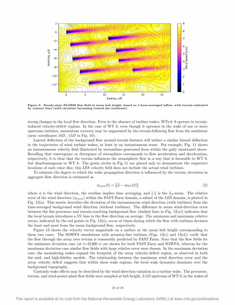
Figure 9. Steady-state FLORIS flow field at mean hub height, based on 1-hour-averaged inflow, with terrain indicatedby contour lines (with elevation increasing toward the southeast).

strong changes in the local flow direction. Even in the absence of turbine wakes, WTs 6–9 operate in terrain-induced velocity-deficit regions. In the case of WT 9, even though it operates in the wake of one or moreupstream turbines, momentum recovery may be augmented by the terrain-following flow from the southwest(near coordinates 10D, -15D in Fig. 10).

Lateral deflection of the background flow around terrain features will induce a similar lateral deflectionin the trajectories of wind turbine wakes, at least in an instantaneous sense. For example, Fig. 11 showsan instantaneous velocity field illustrated by streamlines generated from within the gully mentioned above.Recalling that convergence or divergence of streamlines corresponds to flow acceleration and deceleration,respectively, it is clear that the terrain influences the atmospheric flow in a way that is favorable to WT 9,but disadvantageous to WT 8. The green circles in Fig 11 are placed only to demonstrate the respectivelocations of each rotor disc; this LES velocity field does not include the actual wind turbines.

To estimate the degree to which the wake propagation direction is influenced by the terrain, deviation inaggregate flow direction is estimated as

φerror(t) =∥∥φ− φWT(t)

∥∥ (2)

where φ is the wind direction, the overline implies time averaging, and ‖·‖ is the L2-norm. The relativeerror of the wind direction (φerror) within the FAST.Farm domain, a subset of the LES domain, is plotted inFig. 12(a). This metric describes the deviation of the instantaneous wind direction (with turbines) from thetime-averaged background wind direction (without turbines). The difference in mean wind-direction errorbetween the flat-precursor and terrain-resolving background flow (dashed lines in Fig. 12(a)) indicates thatthe local terrain introduces a 5% bias to the flow direction on average. The minimum and maximum relativeerrors, indicated by the red points in Fig. 12(a), occur at times during which the flow with turbines deviatesthe least and most from the mean background flow, respectively.

Figure 13 shows the velocity vector magnitude on a surface at the mean hub height corresponding tothese two cases. The SOWFA simulations with actuator-line turbines (Figs. 13(c) and 13(d)) verify thatthe flow through the array over terrain is reasonably predicted by FAST.Farm. Note that the flow fields forthe minimum deviation case (at t=21200 s) are shown for both FAST.Farm and SOWFA, whereas for themaximum deviation case similar flow fields with large relative error were chosen. In the maximum deviationcase, the meandering wakes expand the footprint of the array velocity-deficit region, as observed in boththe mid- and high-fidelity models. The relationship between the maximum wind direction error and thearray velocity deficit suggests that within these wake regions, the local wake dynamics dominate over thebackground topography.

Unsteady wake effects may be described by the wind-direction variation in a turbine wake. The precursor,terrain, and wind-power-plant flow fields were sampled at hub height, 2.5D upstream of WT 9, in the wakes of

13 of 18


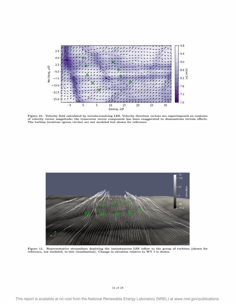
Figure 10. Velocity field calculated by terrain-resolving LES. Velocity direction vectors are superimposed on contoursof velocity vector magnitude; the transverse vector component has been exaggerated to demonstrate terrain effects.The turbine locations (green circles) are not modeled but shown for reference.

Figure 11. Representative streamlines depicting the instantaneous LES inflow to the group of turbines (shown forreference, not modeled, in this visualization). Change in elevation relative to WT 1 is shown.

14 of 18


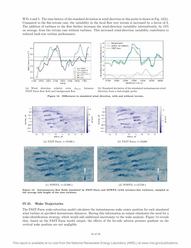
WTs 4 and 5. The time history of the standard deviation in wind direction at this probe is shown in Fig. 12(b).Compared to the flat-terrain case, the variability in the local flow over terrain is increased by a factor of 3.The addition of turbines to the flow further increases the wind-direction variability intermittently, by 15%on average, from the terrain case without turbines. This increased wind-direction variability contributes toreduced back-row turbine performance.

(a) Wind direction relative error φerror betweenFAST.Farm flow field and background flow.

(b) Standard deviation of the simulated instantaneous winddirection from a hub-height probe.

Figure 12. Differences in simulated wind direction, with and without terrain.

(a) FAST.Farm, t=21200 s (b) FAST.Farm, t=24200

(c) SOWFA, t=21200 s (d) SOWFA, t=21730 s

Figure 13. Instantaneous flow fields simulated by FAST.Farm and SOWFA (with actuator-line turbines), sampled atthe average hub height of the nine turbines.

IV.D. Wake Trajectories

The FAST.Farm wake-advection model calculates the instantaneous wake center position for each simulatedwind turbine at specified downstream distances. Having this information as output eliminates the need for awake-identification strategy, which would add additional uncertainty to the wake analysis. Figure 14 revealsthat, based on the FAST.Farm model output, the effects of the lee-side adverse pressure gradient on thevertical wake position are not negligible.

15 of 18


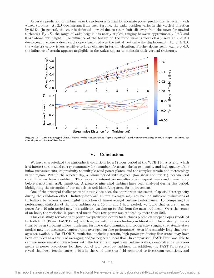
Accurate prediction of turbine wake trajectories is crucial for accurate power predictions, especially withwaked turbines. At 2D downstream from each turbine, the wake position varies in the vertical directionby 0.1D. (In general, the wake is deflected upward due to rotor-shaft tilt away from the tower for upwindturbines.) By 4D, the range of wake heights has nearly tripled, ranging between approximately 0.2D and0.5D above hub height. The influence of the terrain on the rotor wake is most clearly seen at x < 3Ddownstream, where a downward slope clearly reduces the initial vertical wake displacement. For x ≥ 3D,the wake trajectory is less sensitive to large changes in terrain elevation. Further downstream, e.g., x > 6D,the influence of terrain appears negligible as the wakes appear to maintain their vertical trajectory.

Figure 14. Time-averaged FAST.Farm wake trajectories (open symbols) and corresponding terrain slope, colored bythe slope at the turbine base.

V. Conclusions

We have characterized the atmospheric conditions for a 12-hour period at the WFIP2 Physics Site, whichis of interest to the wind energy community for a number of reasons: the large quantity and high quality of theinflow measurements, its proximity to multiple wind power plants, and the complex terrain and meteorologyin the region. Within the selected day, a 1-hour period with atypical (low shear and low TI), near-neutralconditions has been identified. This period of interest occurs after a wind-speed ramp and immediatelybefore a nocturnal ABL transition. A group of nine wind turbines have been analyzed during this period,highlighting the strengths of our models as well identifying areas for improvement.

One of the principal challenges in this study has been the appropriate treatment of spatial heterogeneityduring the validation effort. Industry-standard 10-min averages may not include sufficient realizations ofturbulence to recover a meaningful prediction of time-averaged turbine performance. By comparing theperformance statistics of the nine turbines for a 10-min and 1-hour period, we found that errors in meanpower for a 10-min period may be significant, varying up to 15% from the measured mean. Over the courseof an hour, the variation in predicted mean front-row power was reduced by more than 50%.

This case study revealed that power overprediction occurs for turbines placed on steeper slopes (modeledby both FLORIS and FAST.Farm), which agrees with previous findings in literature. The unsteady interac-tions between turbulent inflow, upstream turbine wake dynamics, and topography suggest that steady-statemodels may not accurately capture time-averaged turbine performance—even if reasonably long time aver-ages are available. For FLORIS simulations including terrain, high-power-producing flow states may havebeen excluded as a result of averaging and/or neglected local flow. In comparison, FAST.Farm was able tocapture more realistic interactions with the terrain and upstream turbine wakes, demonstrating improve-ments in power predictions for three out of four back-row turbines. In addition, the FAST.Farm resultsreveal that local terrain causes a bias in the wind direction field compared to freestream conditions, and

16 of 18


significantly increases variability in the local wind direction. Both of these effects are expected to have animpact on turbine power production and loads. Even though only qualitative comparisons between SOWFAand FAST.Farm are possible at the moment, the preliminary SOWFA results suggest that FAST.Farm isable to capture realistic wake evolution over complex terrain. Future work will simulate the full hour ofinterest with actuator lines, enabling direct quantitative comparisons between all three models.

The value of FLORIS lies in its computational efficiency and applicability to wind-power-plant controland layout optimizations. Optimal control schemes and wind plant layouts determined by FLORIS will notnecessarily be suboptimal, but conservative underpredictions of power are possible based on our findingsregarding time averaging and unsteady effects. In addition, adverse pressure-gradient effects are not neces-sarily negligible, as we have found that the turbine wakes do have a tendency to follow downsloping terrainfor up to 3D. Our FAST.Farm results suggest that an appropriate terrain-resolved inflow field can offerinsights into the instantaneous power production of turbines within a wind plant, at significantly reducedcomputational cost compared to SOWFA, with mean power predictions that are as good as or better thanFLORIS. However, the variability in power output is lower than the SCADA measurements. Without know-ing the instantaneous yaw position of each turbine, the source of variability over the 1-hour period—eitheraerodynamics or yaw misalignment—will not be known with absolute certainty. In addition, FAST.Farmmay overpredict the advection velocity as a consequence of the implemented averaging technique that ac-commodates terrain. By neglecting near-surface cells, the terrain elevation and near-surface flow velocityare artificially increased. This may contribute to the errors noted for turbines on relatively steep windwardslopes.

Acknowledgments

Many thanks to Kelsey Shaler for her FAST.Farm support and to Emmanuel Branlard who developedthe FAST model used in this effort. Also, to Patrick Hawbecker and Julie Lundquist, who provided guidancewith interpreting the WFIP2 measurements.

This work was authored by the National Renewable Energy Laboratory, operated by Alliance for Sustain-able Energy, LLC, for the U.S. Department of Energy (DOE) under Contract No. DE-AC36-08GO28308.Funding provided by the U.S. Department of Energy Office of Energy Efficiency and Renewable EnergyWind Energy Technologies Office. The views expressed in the article do not necessarily represent the viewsof the DOE or the U.S. Government. The U.S. Government retains and the publisher, by accepting thearticle for publication, acknowledges that the U.S. Government retains a nonexclusive, paid-up, irrevocable,worldwide license to publish or reproduce the published form of this work, or allow others to do so, for U.S.Government purposes.

References

1U.S. Department of Energy, “Wind Vision: A New Era for Wind Power in the United States,” Tech. Rep. DOE/GO-102015-4557, DOE Office of Energy Efficiency and Renewable Energy, Washington D.C., 2015.

2Fleming, P., Annoni, J., Scholbrock, A., Quon, E., Dana, S., Schreck, S., Raach, S., Haizmann, F., and Schlipf, D.,“Full-Scale Field Test of Wake Steering,” Wake Conference 2017 , Visby, Sweden, May 2017.

3Yang, X., Pakula, M., and Sotiropoulos, F., “Large-Eddy Simulation of a Utility-Scale Wind Farm in Complex Terrain,”Applied Energy, Vol. 229, Nov. 2018, pp. 767–777.

4Berg, J., Troldborg, N., Sørensen, N., Patton, E., and Sullivan, P., “Large-Eddy Simulation of Turbine Wake in ComplexTerrain,” Journal of Physics: Conference Series, Vol. 854, No. 012003, 2017.

5Quon, E., Churchfield, M. J., Cheung, L., and Kern, S., “Development of a Wind Plant Large-Eddy Simulationwith Measurement-Driven Atmospheric Inflow,” AIAA SciTech 2017 , American Institute of Aeronautics and Astronautics,Grapevine, Texas, Jan. 2017.

6Wilczak, J., Finley, C., Freedman, J., Cline, J., Bianco, L., Olson, J., Djalalova, I., Sheridan, L., Ahlstrom, M.,Manobianco, J., Zack, J., Carley, J. R., Benjamin, S., Coulter, R., Berg, L. K., Mirocha, J., Clawson, K., Natenberg, E.,and Marquis, M., “The Wind Forecast Improvement Project (WFIP): A Public–Private Partnership Addressing Wind EnergyForecast Needs,” Bulletin of the American Meteorological Society, Vol. 96, No. 10, Oct. 2015, pp. 1699–1718.

7Annoni, J., Fleming, P., Scholbrock, A., Roadman, J., Dana, S., Adcock, C., Porte-Agel, F., Raach, S., Haizmann, F., andSchlipf, D., “Analysis of Control-Oriented Wake Modeling Tools Using Lidar Field Results,” Wind Energy Science Discussions,Feb. 2018, pp. 1–17.

8Wu, X., “Inflow Turbulence Generation Methods,” Annual Review of Fluid Mechanics, Vol. 49, No. 1, 2017, pp. 23–49.9Gopalan, H., Gundling, C., Brown, K., Roget, B., Sitaraman, J., Mirocha, J. D., and Miller, W. O., “A Coupled

Mesoscale–Microscale Framework for Wind Resource Estimation and Farm Aerodynamics,” Journal of Wind Engineering andIndustrial Aerodynamics, Vol. 132, Sept. 2014, pp. 13–26.

17 of 18


10Rodrigo, J. S., Arroyo, R. C., Gancarski, P., Guillen, F. B., Avila, M., Barcons, J., Folch, A., Cavar, D., D Allaerts,Meyers, J., and Dutrieux, A., “Comparing Meso-Micro Methodologies for Annual Wind Resource Assessment and TurbineSiting at Cabauw,” J. Phys.: Conf. Ser., Vol. 1037, No. 7, 2018, pp. 072030.

11Politis, E. S., Prospathopoulos, J., Cabezon, D., Hansen, K. S., Chaviaropoulos, P. K., and Barthelmie, R. J., “ModelingWake Effects in Large Wind Farms in Complex Terrain: The Problem, the Methods and the Issues: Wake Effects in LargeWind Farms in Complex Terrain,” Wind Energy, Vol. 15, No. 1, Jan. 2012, pp. 161–182.

12Shamsoddin, S. and Porte-Agel, F., “Large-Eddy Simulation of Atmospheric Boundary-Layer Flow Through a WindFarm Sited on Topography,” Boundary-Layer Meteorology, Vol. 163, No. 1, April 2017, pp. 1–17.

13Ma, Y. and Liu, H., “Large-Eddy Simulations of Atmospheric Flows Over Complex Terrain Using the Immersed-BoundaryMethod in the Weather Research and Forecasting Model,” Boundary-Layer Meteorology, Vol. 165, No. 3, Dec. 2017, pp. 421–445.

14NASA JPL, “NASA Shuttle Radar Topography Mission Global 1 Arc Second,” 2013.15Churchfield, M. J., Lee, S., Moriarty, P. J., Martinez, L. A., Leonardi, S., Vijayakumar, G., and Brasseur, J. G., “A

Large-Eddy Simulation of Wind-Plant Aerodynamics,” 50th AIAA Aerospace Sciences Meeting, Nashville, Tennessee, Jan.2012.

16Haupt, S., Anderson, A., Berg, L., Brown, B., Churchfield, M., Draxl, C., Kalb, C., Koo, E., Kosovic, B., Kotamarthi,R., Mazzaro, L., Mirocha, J., Quon, E., Rai, R., and Sever, G., “Third-Year Report of the Atmosphere to Electrons Mesoscale-to-Microscale Coupling Project,” Tech. rep., Pacific Northwest National Laboratory, Dec. 2017.

17Wharton, S. and Lundquist, J. K., “Atmospheric Stability Affects Wind Turbine Power Collection,” Environ. Res. Lett.,Vol. 7, No. 1, 2012, pp. 014005.

18Wharton, S. and Lundquist, J. K., “Assessing Atmospheric Stability and Its Impacts on Rotor-Disk Wind Characteristicsat an Onshore Wind Farm: Atmospheric Stability on Rotor-Disk Wind Characteristics,” Wind Energy, Vol. 15, No. 4, May2012, pp. 525–546.

19Gebraad, P. M. O., Teeuwisse, F. W., van Wingerden, J. W., Fleming, P. A., Ruben, S. D., Marden, J. R., and Pao,L. Y., “Wind Plant Power Optimization through Yaw Control Using a Parametric Model for Wake Effects—a CFD SimulationStudy,” Wind Energ., Vol. 19, No. 1, Jan. 2016, pp. 95–114.

20Jonkman, J. M., Annoni, J., Hayman, G., Jonkman, B., and Purkayastha, A., “Development of FAST.Farm: A NewMulti-Physics Engineering Tool for Wind-Farm Design and Analysis,” 35th Wind Energy Symposium, American Institute ofAeronautics and Astronautics, Grapevine, Texas, Jan. 17.

21Shamsoddin, S. and Porte-Agel, F., “Wind Turbine Wakes over Hills,” Journal of Fluid Mechanics, Vol. 855, Nov. 2018,pp. 671–702.

22Martınez-Tossas, L. A., Annoni, J., Fleming, P. A., and Churchfield, M. J., “The Aerodynamics of the Curled Wake: ASimplified Model in View of Flow Control,” Wind Energy Science Discussions, Aug. 2018, pp. 1–17.

23“OpenFAST Documentation,” \url{http://openfast.readthedocs.io/en/master/}, Nov. 2017.24Han, Y., Stoellinger, M., and Naughton, J., “Large Eddy Simulation for Atmospheric Boundary Layer Flow over Flat

and Complex Terrains,” Journal of Physics: Conference Series, Vol. 753, Sept. 2016, pp. 032044.25Quon, E. W., Ghate, A. S., and Lele, S. K., “Enrichment Methods for Inflow Turbulence Generation in the Atmospheric

Boundary Layer,” J. Phys.: Conf. Ser., Vol. 1037, No. 7, 2018, pp. 072054.26Lohner, R. and Yang, C., “Improved ALE Mesh Velocities for Moving Bodies,” Communications in Numerical Methods

in Engineering, Vol. 12, No. 10, 1996, pp. 599–608.

18 of 18


Documents

Validation of Wind Power Plant Modeling Approaches in