Embed Size (px)
Citation preview
Valuation of Guaranteed Minimum Maturity Benefits in
variable annuities with surrender options
Jonathan Ziveyi1
Joint work with Michael Sherris2
and Yang Shen3
ASTIN, AFIR/ERM and IACA Colloquia
1Risk & Actuarial Studies, UNSW Business School, UNSW Australia.2CEPAR, Risk & Actuarial Studies, UNSW Australia3CEPAR, Risk & Actuarial Studies, UNSW Australia
1/26

Outline of the Presentation
Basics
Motivation
The problem statement
General solution
Numerical implementation
Numerical results
2/26
Basics
A variable annuity is a contract between an insurance company and apolicyholder.
The insurance company agrees to make periodic payments to thepolicyholder in future (mainly post retirement).
The policyholder purchases a variable annuity by paying either asingle premium payment or a series of payments.
Unlike traditional mutual funds and life insurance products, variableannuity contracts come with embedded guarantees which protect thepolicyholder’s savings against unanticipated outcomes.
Some of the advantages of variable annuities include
Tax-deferred earnings,Tax-free transfers across a variety of investment options,Death benefit protection options,Living benefit protection options,Lifetime income options.
3/26
Basics cont..
Variable annuities fulfill the social needs for the aging population byproviding products that deliver certainty of income upon retirement.Guarantees can be underwritten for the accumulation phase, annuityphase or untimely death of the policyholder, and they fall into twomajor groups i.e. GMDB and GMLB.GMLB can further be categorized into GMxB where where x standsfor maturity (M), income (I ) and withdrawal (W ).These guarantees exhibit financial option-like features, naturallyleading to the way they are valued in practise.Premiums paid when purchasing variable annuities are usuallyinvested in various subaccounts with different characteristics andinvestment strategies.Variable annuity subaccounts include actively managed portfolios,exchange-traded funds, index-linked portfolios alternative investmentsand other quantitative-driven strategies.Insurance companies usually charge proportional fees on variableannuity contracts as a way of funding the guarantees.
4/26

Basics cont..
If the fees are too high relative to the performance of the fund, thepolicyholder can choose to surrender the contract or the guaranteeprior to maturity in return of a surrender benefit.
The benefits will be net of surrender/penalty charges enforced as away of discouraging early termination of the contract.
We focus on the valuation of the GMMB rider embedded in a variableannuity contract in the case where the guarantee can be surrenderedanytime prior to maturity.
Shen and Xu (2005) formulate the valuation problem for equity-linkedpolicies with interest rate guarantees in the presence of surrenderoptions as a free-boundary problem which can be solved by usingfinite difference techniques.
Constabile et al. (2008) consider a similar valuation problem anddevise the binomial trees approach to generate fair premium values.
5/26
Motivation
Bauer et al. (2008) provide a general framework for consistent pricingof various types of guarantees embedded in variable annuities whichare currently traded in the market.
They present an extensive analysis of the guarantees by incorporatingthe possibility of surrendering the contracts anytime prior to maturity.
Bacinello (2013) considers the pricing of participating life insurancepolicies with surrender options using recursive binomial treesapproach.
Bernard et al. (2014) use American style option pricing techniquesdeveloped in Carr et al. (1992) to derive the representation of theoptimal surrender strategy for a variable annuity contract embeddedwith guaranteed minimum accumulation benefits (GMAB).
The authors treat the entire variable annuity contract (the mutualfund plus the GMAB) as a single underlying asset and then derive thecorresponding pricing formulas.
6/26
Key Results
In this paper, we provide alternative derivations and representation ofthe GMMB embedded in a variable annuity contract that can besurrendered early by exploiting techniques devised in Jamshidian(1992).
Using well established arguments developed in Jacka (1991), Myneni(1992) and El Karoui & Karatzas (1993), we transform the stoppingtime problem into a free-boundary problem leading to an equivalentrepresentation in Shen and Xu (2005).
Our main results involve the derivation of integral expressions for theguarantee values, early exercise boundaries and deltas for the GMMBby using Jamshidian (1992) techniques to transform the free-boundaryproblem to a non-homogeneous partial differential equation (PDE)which we later solve with the aide of Duhamels principle.
7/26
The Asset and Fund Dynamics
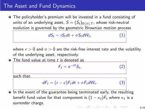
The policyholder’s premium will be invested in a fund consisting ofunits of an underlying asset, S = (St)0≤t≤T , whose risk-neutralevolution is governed by the geometric Brownian motion process
dSt = rStdt + σStdWt , (1)
where r > 0 and σ > 0 are the risk-free interest rate and the volatilityof the underlying asset, respectively.The fund value at time t is denoted as
Ft = e−ct
St , (2)
such that
dFt = (r − c)Ftdt + σFtdWt . (3)
In the event of the guarantee being terminated early, the resultingbenefit fund value for that component is (1− κt)Ft where κt is asurrender charge.
8/26

Problem Statement
We assume an exponentially decreasing surrender fee structure on theguarantee implying that the fund value of the guarantee component is(1− κt)Ft = e−κ(T−t)Ft .
The variable annuity contract at anytime prior to maturity can thenbe represented as
Ft = e−r(T−t)
E [FT ] (4)
+ ess supt≤τ
∗≤T
e−r(τ∗−t)
E
[
max(GT − e−κ(T−τ
∗)Fτ∗ , 0)|Ft
]
,
where the supremum is taken over all stopping times, τ∗.
The first component on the right-hand side of equation (4) is thediscounted expectation of maturity value of the fund which can beevaluated easily using a variety of techniques such as the equilibriumasset pricing theory.
The second component is a typical American put option and we willdenote this by C (t,F ).
9/26
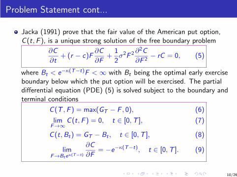
Problem Statement cont...
Jacka (1991) prove that the fair value of the American put option,C (t,F ), is a unique strong solution of the free boundary problem
∂C
∂t+ (r − c)F
∂C
∂F+
1
2σ2
F2∂
2C
∂F 2− rC = 0, (5)
where Bt < e−κ(T−t)F < ∞ with Bt being the optimal early exerciseboundary below which the put option will be exercised. The partialdifferential equation (PDE) (5) is solved subject to the boundary andterminal conditions
C (T ,F ) = max(GT − F , 0), (6)
limF→∞
C (t,F ) = 0, t ∈ [0,T ], (7)
C (t,Bt) = GT − Bt , t ∈ [0,T ], (8)
limF→Bte
κ(T−t)
∂C
∂F= −e
−κ(T−t), t ∈ [0,T ]. (9)
10/26

Solution Procedure
The underlying asset domain for the PDE (5) is bounded below by the earlyexercise boundary, Bt .
Jamshidian (1992) shows that one can consider an unbounded domain forthe underlying asset by noting that at anytime, t ∈ [0,T ], below the earlyexercise boundary
C (t,F ) = GT − e−κ(T−t)
Ft , (10)
implying that the following equation holds
∂C
∂t+ (r − c)F
∂C
∂F+
1
2σ2
F2 ∂
2C
∂F 2− rC
= (c − κ)e−κ(T−t)F − rGT . (11)
Combining equations (5) and (11), and using the fact that C (t,F ) is acontinuous differentiable function in F at Bt yields
∂C
∂t+ (r − c)F
∂C
∂F+
1
2σ2
F2 ∂
2C
∂F 2− rC (12)
+ 1{F≤Bteκ(T−t)}
[
rGT − (c − κ)e−κ(T−t)F
]
= 0,
11/26
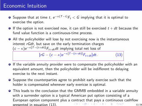
Economic Intuition
Suppose that at time t, e−κ(T−t)Ft < G implying that it is optimal toexercise the option.
If the option is not exercised now, it can still be exercised t + dt because thefund value function is a continuous-time process.
All the policyholder will lose by not exercising now is the instantaneousinterest rGdt, but save on the early termination charges(c − κ)e−κ[T−(t+dt)]Ft+dtdt implying total net loss of
[rG − (c − κ)e−κ[T−(t+dt)]Ft+dt ]dt. (13)
If the variable annuity provider were to compensate the policyholder with anequivalent amount, then the policyholder will be indifferent to delayingexercise to the next instant.
Suppose the counterparties agree to prohibit early exercise such that theholder is compensated whenever early exericse is optimal.
This leads to the conclusion that the GMMB embedded in a variable annuitywith a surrender option is a typical American put option consisting of aEuropean option component plus a contract that pays a continuous cashflowpresented in equation (13). 12/26
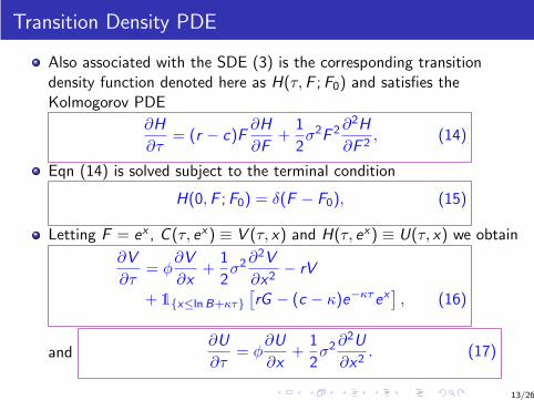
Transition Density PDE
Also associated with the SDE (3) is the corresponding transitiondensity function denoted here as H(τ,F ;F0) and satisfies theKolmogorov PDE
∂H
∂τ= (r − c)F
∂H
∂F+
1
2σ2
F2∂
2H
∂F 2, (14)
Eqn (14) is solved subject to the terminal condition
H(0,F ;F0) = δ(F − F0), (15)
Letting F = ex , C (τ, ex) ≡ V (τ, x) and H(τ, ex) ≡ U(τ, x) we obtain
∂V
∂τ= φ
∂V
∂x+
1
2σ2∂
2V
∂x2− rV
+ 1{x≤lnB+κτ}
[
rG − (c − κ)e−κτex]
, (16)
and∂U
∂τ= φ
∂U
∂x+
1
2σ2∂
2U
∂x2. (17)
13/26
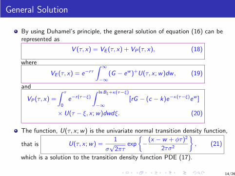
General Solution
By using Duhamel’s principle, the general solution of equation (16) can berepresented as
V (τ, x) = VE (τ, x) + VP(τ, x), (18)
where
VE (τ, x) = e−rτ
∫ ∞
−∞
(G − ew )+U(τ, x ;w)dw , (19)
and
VP(τ, x) =
∫ τ
0
e−r(τ−ξ)
∫ lnBξ+κ(τ−ξ)
−∞
[rG − (c − k)e−κ(τ−ξ)ew ]
× U(τ − ξ, x ;w)dwdξ. (20)
The function, U(τ, x ;w) is the univariate normal transition density function,
that is U(τ, x ;w) =1
σ√2πτ
exp
{
− (x − w + φτ)2
2τσ2
}
, (21)
which is a solution to the transition density function PDE (17).
14/26
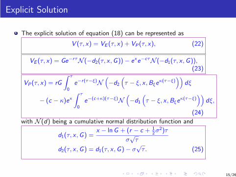
Explicit Solution
The explicit solution of equation (18) can be represented as
V (τ, x) = VE (τ, x) + VP(τ, x), (22)
VE (τ, x) = Ge−rτN (−d2(τ, x ,G ))− e
xe−cτN (−d1(τ, x ,G )),
(23)
VP(τ, x) = rG
∫ τ
0
e−r(τ−ξ)N
(
−d2
(
τ − ξ, x ,Bξeκ(τ−ξ)
))
dξ
− (c − κ)ex∫ τ
0
e−(c+κ)(τ−ξ)N
(
−d1
(
τ − ξ, x ,Bξeκ(τ−ξ)
))
dξ,
(24)
with N (d) being a cumulative normal distribution function and
d1(τ, x ,G ) =x − lnG + (r − c + 1
2σ2)τ
σ√τ
d2(τ, x ,G ) = d1(τ, x ,G )− σ√τ . (25)
15/26
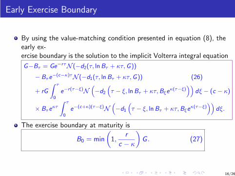
Early Exercise Boundary
By using the value-matching condition presented in equation (8), theearly ex-ercise boundary is the solution to the implicit Volterra integral equation
G−Bτ = Ge−rτN (−d2(τ, lnBτ + κτ,G ))
− Bτe−(c−κ)τN (−d1(τ, lnBτ + κτ,G )) (26)
+ rG
∫ τ
0
e−r(τ−ξ)N
(
−d2
(
τ − ξ, lnBτ + κτ,Bξeκ(τ−ξ)
))
dξ − (c − κ)
× Bτeκτ
∫ τ
0
e−(c+κ)(τ−ξ)N
(
−d1
(
τ − ξ, lnBτ + κτ,Bξeκ(τ−ξ)
))
dξ.
The exercise boundary at maturity is
B0 = min
(
1,r
c − κ
)
G . (27)
16/26
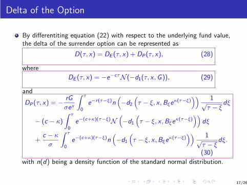
Delta of the Option
By differentiting equation (22) with respect to the underlying fund value,the delta of the surrender option can be represented as
D(τ, x) = DE (τ, x) + DP(τ, x), (28)
where
DE (τ, x) = −e−cτN (−d1(τ, x ,G )), (29)
and
DP(τ, x) = − rG
σex
∫ τ
0
e−r(τ−ξ)
n
(
−d2
(
τ − ξ, x ,Bξeκ(τ−ξ)
)) 1√τ − ξ
dξ
− (c − κ)
∫ τ
0
e−(c+κ)(τ−ξ)N
(
−d1
(
τ − ξ, x ,Bξeκ(τ−ξ)
))
dξ
+c − κ
σ
∫ τ
0
e−(c+κ)(τ−ξ)
n
(
−d1
(
τ − ξ, x ,Bξeκ(τ−ξ)
)) 1√τ − ξ
dξ.
(30)
with n(d) being a density function of the standard normal distribution.
17/26
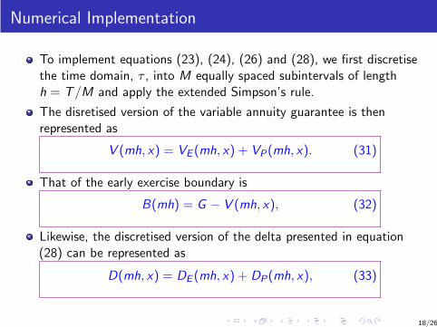
Numerical Implementation
To implement equations (23), (24), (26) and (28), we first discretisethe time domain, τ , into M equally spaced subintervals of lengthh = T/M and apply the extended Simpson’s rule.
The disretised version of the variable annuity guarantee is thenrepresented as
V (mh, x) = VE (mh, x) + VP(mh, x). (31)
That of the early exercise boundary is
B(mh) = G − V (mh, x), (32)
Likewise, the discretised version of the delta presented in equation(28) can be represented as
D(mh, x) = DE (mh, x) + DP(mh, x), (33)
18/26
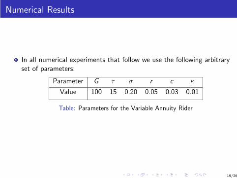
Numerical Results
In all numerical experiments that follow we use the following arbitraryset of parameters:
Parameter G τ σ r c κ
Value 100 15 0.20 0.05 0.03 0.01
Table: Parameters for the Variable Annuity Rider
19/26
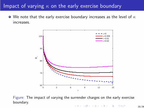
Impact of varying κ on the early exercise boundary
We note that the early exercise boundary increases as the level of κincreases.
τ
0 3 6 9 12 15
Bτ
60
70
80
90
100κ=0κ=0.005κ=0.01κ=0.02
Figure: The impact of varying the surrender charges on the early exerciseboundary.
20/26
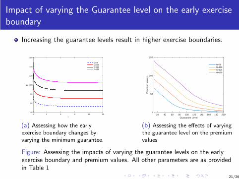
Impact of varying the Guarantee level on the early exercise
boundary
Increasing the guarantee levels result in higher exercise boundaries.
τ
0 3 6 9 12 15
Bτ
40
60
80
100
120
140
160
G=75G=100G=125G=150
(a) Assessing how the early
exercise boundary changes by
varying the minimum guarantee.
Guarantee Level20 40 60 80 100 120 140 160 180 200
Pre
miu
m V
alue
s
0
50
100
150
G=75G=100G=125G=150
(b) Assessing the effects of varying
the guarantee level on the premium
values
Figure: Assessing the impacts of varying the guarantee levels on the earlyexercise boundary and premium values. All other parameters are as providedin Table 1
21/26
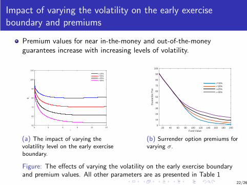
Impact of varying the volatility on the early exercise
boundary and premiums
Premium values for near in-the-money and out-of-the-moneyguarantees increase with increasing levels of volatility.
τ
0 3 6 9 12 15
Bτ
50
60
70
80
90
100
110
σ=15%σ=20%σ=25%σ=30%
(a) The impact of varying the
volatility level on the early exercise
boundary.
Fund Value20 40 60 80 100 120 140 160 180 200
Gua
rant
ee F
ee
0
10
20
30
40
50
60
70
80
90
100
σ=15%
σ=20%σ=25%
σ=30%
(b) Surrender option premiums for
varying σ.
Figure: The effects of varying the volatility on the early exercise boundaryand premium values. All other parameters are as presented in Table 1
22/26

Impact of varying interest rate levels on the early exercise
boundary and premiums
The rule of thumb when trading put options is that higher risk freeinterest rates mean cheaper put option prices, all things being equal.
τ
0 3 6 9 12 15
Bτ
55
60
65
70
75
80
85
90
95
100
r=3%r=4%r=4.5%r=5%
(a) The impact of varying interest
rates on the early exercise
boundary.
Fund Value20 40 60 80 100 120 140 160 180 200
Gua
rant
ee F
ee
0
10
20
30
40
50
60
70
80
90
100
r=3%
r=4%
r=5%
(b) The impact of varying interest
rates on guarantee premiums.
Figure: The effects of varying interest rates on the early exercise boundaryand premium values. All other parameters are as presented in Table 1
23/26
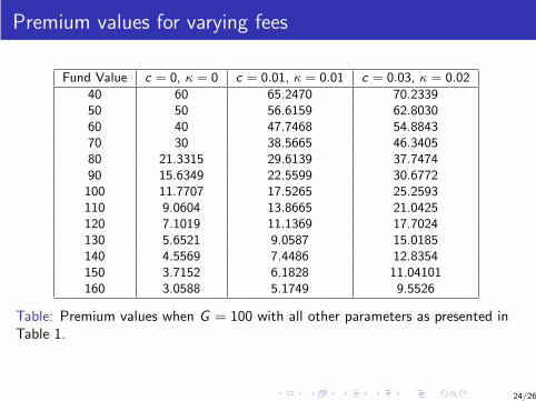
Premium values for varying fees
Fund Value c = 0, κ = 0 c = 0.01, κ = 0.01 c = 0.03, κ = 0.02
40 60 65.2470 70.2339
50 50 56.6159 62.8030
60 40 47.7468 54.8843
70 30 38.5665 46.3405
80 21.3315 29.6139 37.7474
90 15.6349 22.5599 30.6772
100 11.7707 17.5265 25.2593
110 9.0604 13.8665 21.0425
120 7.1019 11.1369 17.7024
130 5.6521 9.0587 15.0185
140 4.5569 7.4486 12.8354
150 3.7152 6.1828 11.04101
160 3.0588 5.1749 9.5526
Table: Premium values when G = 100 with all other parameters as presented inTable 1.
24/26
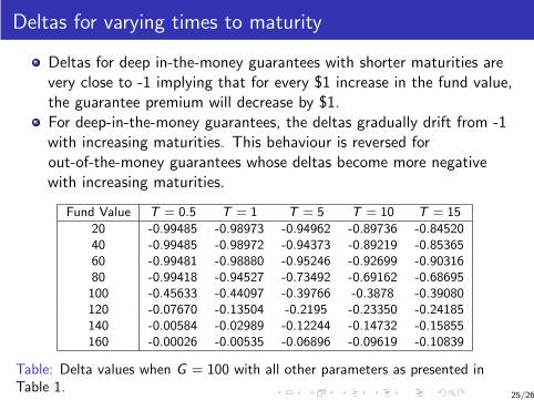
Deltas for varying times to maturity
Deltas for deep in-the-money guarantees with shorter maturities arevery close to -1 implying that for every $1 increase in the fund value,the guarantee premium will decrease by $1.For deep-in-the-money guarantees, the deltas gradually drift from -1with increasing maturities. This behaviour is reversed forout-of-the-money guarantees whose deltas become more negativewith increasing maturities.
Fund Value T = 0.5 T = 1 T = 5 T = 10 T = 15
20 -0.99485 -0.98973 -0.94962 -0.89736 -0.84520
40 -0.99485 -0.98972 -0.94373 -0.89219 -0.85365
60 -0.99481 -0.98880 -0.95246 -0.92699 -0.90316
80 -0.99418 -0.94527 -0.73492 -0.69162 -0.68695
100 -0.45633 -0.44097 -0.39766 -0.3878 -0.39080
120 -0.07670 -0.13504 -0.2195 -0.23350 -0.24185
140 -0.00584 -0.02989 -0.12244 -0.14732 -0.15855
160 -0.00026 -0.00535 -0.06896 -0.09619 -0.10839
Table: Delta values when G = 100 with all other parameters as presented inTable 1.
25/26

Questions and Comments?
26/26