Full Terms & Conditions of access and use can be found athttp://www.tandfonline.com/action/journalInformation?journalCode=ujrs20

Download by: [Ghent University] Date: 06 April 2016, At: 01:00

Canadian Journal of Remote SensingJournal canadien de télédétection

ISSN: 0703-8992 (Print) 1712-7971 (Online) Journal homepage: http://www.tandfonline.com/loi/ujrs20

Hyperspectral Image Denoising with a CombinedSpatial and Spectral Weighted Hyperspectral TotalVariation Model

Cheng Jiang, Hongyan Zhang, Liangpei Zhang, Huanfeng Shen & QiangqiangYuan

To cite this article: Cheng Jiang, Hongyan Zhang, Liangpei Zhang, Huanfeng Shen &Qiangqiang Yuan (2016): Hyperspectral Image Denoising with a Combined Spatial and SpectralWeighted Hyperspectral Total Variation Model, Canadian Journal of Remote Sensing, DOI:10.1080/07038992.2016.1158094

To link to this article: http://dx.doi.org/10.1080/07038992.2016.1158094

Published online: 04 Apr 2016.

Submit your article to this journal

View related articles

View Crossmark data

Canadian Journal of Remote Sensing, 42:1–20, 2016Copyright c© CASIISSN: 0703-8992 print / 1712-7971 onlineDOI: 10.1080/07038992.2016.1158094

Hyperspectral Image Denoising with a Combined Spatialand Spectral Weighted Hyperspectral TotalVariation Model

Cheng Jiang1,4, Hongyan Zhang2,4,*, Liangpei Zhang2,4, Huanfeng Shen3,4,and Qiangqiang Yuan1,4

1School of Geodesy and Geomatics, Wuhan University, 129 Luoyu Road, Wuhan 430079, China2The State Key Laboratory of Information Engineering in Surveying, Mapping, and Remote Sensing,Wuhan University, 129 Luoyu Road, Wuhan 430079, China3School of Resources and Environmental Sciences, Wuhan University, 129 Luoyu Road, Wuhan 430079,China4Collaborative Innovation Center of Geospatial Technology, Wuhan University, 129 Luoyu Road, Wuhan430079, China

Abstract. Hyperspectral image (HSI) denoising is a prerequisite for many subsequent applications. For an HSI, the level and typeof noise often vary with different bands and spatial positions, which make it difficult to effectively remove noise while preservingtextures and edges. To alleviate this problem, we propose a new total-variation model. The main contribution of the proposedapproach lies in that the adaptive regularization terms in both the spatial and the spectral dimensions are designed separately andthen combined into a unified framework. The 2 separate regularization terms allow a better description of the intrinsic natureof the original HSI data and can simultaneously penalize the noise from both the spatial and spectral perspectives. The designedweights for the regularization terms are positively correlated with the magnitude of the noise intensity and negatively correlatedwith the signal variation; thus, the original signal can be accurately retained and the noise can be effectively suppressed. Toefficiently process the HSI, which appears as a huge data cube, a new optimization algorithm based on the alternating directionmethod of multipliers (ADMM) procedure is proposed to solve the new model. Experiments using HYDICE and AVIRIS imageswere conducted to validate the effectiveness of the proposed method.

Resume. Hyperspectrale l’image (HSI) debruitage est une condition prealable pour de nombreuses applications ulterieures.Pour un HSI, le niveau et le type de bruit varie souvent avec differents groupes et positions spatiales, ce qui rend difficiled’eliminer efficacement le bruit tout en preservant les textures et les bords. Pour pallier ce probleme, nous proposons un nouveaumodele de variation totale. Les principales contributions de l’approche proposee mensonge dans la conception des termes deregularisation adaptative dans les deux dimensions spatiales et spectrales, et en les combinant dans un cadre unifie. Les deuxtermes de regularisation separes permettent une meilleure description de la nature intrinseque des donnees HSI original et peuventpenaliser simultanement le bruit a la fois des perspectives spatiales et spectrales. Les poids concus pour les termes de regularisationsont en correlation positive avec la grandeur de l’intensite du bruit et correlation negative avec la variation de signal; ainsi, lesignal d’origine peut etre retenu avec precision et le bruit peut etre efficacement supprimee. Pour traiter efficacement le HSI, quiapparaıt comme un enorme cube de donnees, un nouvel algorithme d’optimisation base sur la methode de direction alternee demultiplicateurs «alternating direction method of multipliers» (ADMM) procedure est proposee pour resoudre le nouveau modele.Des experiences utilisant des images AVIRIS et HYDICE et ont ete menees afin de valider l’efficacite de la methode proposee.

INTRODUCTIONWith their high spectral resolution, hyperspectral images

(HSIs) are commonly used in applications requiring fine identifi-cation of materials or precise estimation of physical parameters.As a result of the physical limitations of the sensors (Zhang et al.2012), HSIs often contain different levels of noise, which notonly affects the visual quality, but also can reduce the accuracy

Received 1 August 2015. Accepted 15 February 2016.*Corresponding author. e-mail: zhanghongyan@whu.edu.cn.

of the subsequent processing, e.g., unmixing (Iordache et al.2012), classification (Harris et al. 2006), clustering (Zhang etal. 2016) and fusion (Jiang et al. 2014). Therefore, with the rapiddevelopment of applications using HSIs, the denoising task isbecoming more and more important.

For gray images, there are a variety of denoising meth-ods, e.g., the total variation (TV) model (Rudin et al. 1992),Gaussian scale mixtures (Portilla et al. 2003), nonlocal means(Buades et al. 2005), wavelets (Selesnick 2002), anisotropicdiffusion (Perona and Malik 1990), and sparse representation(Elad and Aharon 2006). Intuitively, we can apply these meth-

1

Dow

nloa

ded

by [

Ghe

nt U

nive

rsity

] at

01:

00 0

6 A

pril

2016

2 CANADIAN JOURNAL OF REMOTE SENSING/JOURNAL CANADIEN DE TELEDETECTION

ods to an HSI in a band-by-band manner. However, because thestrong correlations between the HSI bands are overlooked, thesemethods often perform poorly. To deal with this problem, someresearchers (Othman and Qian 2006; Chen and Qian 2011) haveproposed to first decorrelate the HSI bands and then successivelyapply denoising methods in both the spatial and spectral dimen-sions. These methods work well when the HSI already has ahigh signal-to-noise ratio (SNR). The redundancy of the spectralbands can also be utilized by subspace-based methods, whichfirst rearrange the HSI into a matrix whose columns contain thespectral signatures and then separate the signal from the noise byestimating the signal subspace (Kuybeda et al. 2007; Acito et al.2010). However, the common approach is to extend the well-known 2-D denoising methods to higher dimensions. For exam-ple, Chen et al. (2011) extended Sendur and Selesnick’s (2002)well-known bivariate wavelet thresholding method from grayimage denoising to HSI denoising with a 3-D wavelet transform;Muti and Bourennane (2007) extended the classic 2-D Wienerfiltering to multidimensional Wiener filtering based on a tensormodel and multilinear algebra; Martın-Herrero (2007) extendedthe 2-D anisotropic diffusion for HSIs with 2 precisely defineddiffusion processes in the spatial and spectral dimensions, re-spectively; and Qian et al. (2012) extended the traditional 2-Dnonlocal means to a 3-D perspective. In recent years, methodsbased on tensor decomposition (Letexier and Bourennane 2008;Liu et al. 2012; Guo et al. 2013; Lin and Bourennane 2013b)and anisotropic diffusion (Mendez-Rial et al. 2010; Wang et al.2010; Mendez-Rial and Martin-Herrero 2012) have been exten-sively studied. In addition, some sophisticated strategies havealso been investigated with new, emerging technologies. For ex-ample, by stacking a local patch of an HSI into a 2-D matrix,Zhang et al. (2014) exploited low-rank matrix recovery theory todenoise the patch. By stacking cubes of voxels into a 4-D group,Maggioni (2013) applied a 4-D transform and collaborative fil-tering for volumetric data denoising and reconstruction. Basedon these existing methods, some hybrid methods have also beeninvestigated, such as combining nonlocal means with sparse rep-resentation (Qian and Ye 2013), wavelet packet transform withTUCKER3 decomposition (Lin and Bourennane 2013a), sparserepresentation with wavelets (Zelinski and Goyal 2006; Rastiet al. 2014), principal component analysis with block matching3-D (Chen et al. 2012) or 4-D filter (Chen et al. 2014), sparserepresentation with low-rank constraint (Zhao and Yang 2015)and TV with low-rank constraint (He et al. 2016).

As a simple but effective model, the TV model has beenwidely used in imaging science, in applications such as im-age restoration, superresolution, segmentation, inpainting, andunmixing. Very recently, the TV model has also been appliedto HSI denoising. For an HSI, there are 2 spatial dimensions(along-track and cross-track) and 1 spectral dimension (wave-length). Yuan et al. (2012) extended the traditional TV model tothe spatial and spectral adaptive hyperspectral TV (SSAHTV)model. The SSAHTV model denoises an HSI with the TV reg-ularization in the spatial dimensions and can adjust the degree

of smoothing on different pixels and different bands with a sin-gle regularization parameter. This model has been proved to bemuch more effective than the procedure that directly appliesthe traditional TV model to each band of the HSI. Althoughthe degree of smoothing can be adjusted in a 3-D manner, themodel is still not a real 3-D TV model without considering thefirst-order difference in the spectral dimension. The later workby Yuan et al. (2014) first applied a 2-D adaptive TV model toan HSI twice, from the front and side views, respectively, andthen adopted a Q-weighting strategy to fuse the 2 results. Theimprovement of this approach is a result of implicitly using theTV regularization in the spectral dimension. In addition, thereare also methods that explicitly adopt the TV regularizationin the spectral dimension, such as the methods proposed in Liet al. (2010) and Zhang (2012); however, the methods proposedin those studies cannot adjust the degree of smoothing, whichcan significantly affect the denoising performance for an HSIwith a nonstationary noise variance. To sum, although the TVmodel has been used for HSI denoising, a 3-D TV model forHSI denoising, which is simple, effective, and can deal with thesignal and noise variation, is still lacking.

In this work, we propose a new combined spatial and spec-tral weighted hyperspectral total variation (CSSWHTV) modelfor HSI denoising. As a 3-D data cube, the HSI is denoised notonly in the spatial dimensions but also in the spectral dimension.The prior model is a combination of 2 separate, finely designedregularization terms that can penalize the variations of pixelsin both the spatial and spectral dimensions. Unlike the existing3-D TV models, the proposed model can automatically adjustthe penalizing strength for the variations of the different pixels.To better attenuate the noise and protect the original information,the weight is designed to be positively correlated with the mag-nitude of the noise intensity and negatively correlated with thesignal variation. To solve the new CSSWHTV model, we pro-pose a fast algorithm based on the alternating direction methodof multipliers (ADMM; Eckstein and Bertsekas 1992; Gabayand Mercier 1976), a method from the augmented Lagrangianfamily. From the experimental results with both simulated andreal-image data, it is shown that the proposed CSSWHTV modelworks well, not only for random noise but also for striping noise(Acito et al. 2011b), which validates the effectiveness of theproposed CSSWHTV method.

The remainder of this article is organized as follows: In “Pro-posed Method,” the proposed CSSWHTV model is introduced.In “Numerical Solution,” we briefly review the ADMM proce-dure, and then the proposed algorithm to solve the CSSWHTVmodel is presented. The experimental results are presented in“Experiments and Discussion.” “Conclusions” concludes thearticle.

PROPOSED METHODMany previous studies (Chen and Qian 2011; Othman and

Qian 2006) have shown that, to acquire better results, the de-noising process should operate not only on the spatial dimen-

Dow

nloa

ded

by [

Ghe

nt U

nive

rsity

] at

01:

00 0

6 A

pril

2016

VOL. 42, NO. 1, FEBRUARY/FEVRIER 2016 3

sions but also on the spectral dimension. Due to the differencein the signal nature of the spatial and the spectral dimensions(Othman and Qian 2006), we chose to first design the corre-sponding weighted TV regularization terms separately and thencombine them effectively.

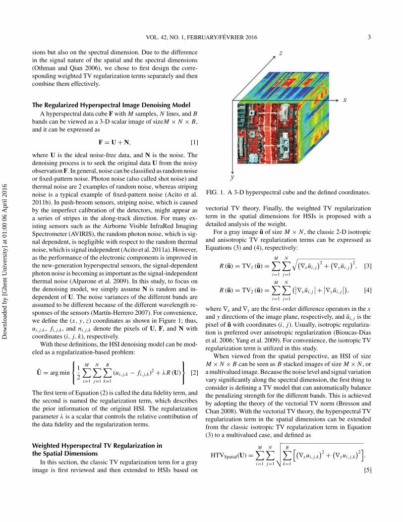
The Regularized Hyperspectral Image Denoising ModelA hyperspectral data cube F with M samples, N lines, and B

bands can be viewed as a 3-D scalar image of sizeM ×N × B,and it can be expressed as

F = U+ N, [1]

where U is the ideal noise-free data, and N is the noise. Thedenoising process is to seek the original data U from the noisyobservation F. In general, noise can be classified as random noiseor fixed-pattern noise. Photon noise (also called shot noise) andthermal noise are 2 examples of random noise, whereas stripingnoise is a typical example of fixed-pattern noise (Acito et al.2011b). In push-broom sensors, striping noise, which is causedby the imperfect calibration of the detectors, might appear asa series of stripes in the along-track direction. For many ex-isting sensors such as the Airborne Visible InfraRed ImagingSpectrometer (AVIRIS), the random photon noise, which is sig-nal dependent, is negligible with respect to the random thermalnoise, which is signal independent (Acito et al. 2011a). However,as the performance of the electronic components is improved inthe new-generation hyperspectral sensors, the signal-dependentphoton noise is becoming as important as the signal-independentthermal noise (Alparone et al. 2009). In this study, to focus onthe denoising model, we simply assume N is random and in-dependent of U. The noise variances of the different bands areassumed to be different because of the different wavelength re-sponses of the sensors (Martın-Herrero 2007). For convenience,we define the (x, y, z) coordinates as shown in Figure 1; thus,ui,j,k , fi,j,k , and ni,j,k denote the pixels of U, F, and N withcoordinates (i, j, k), respectively.

With these definitions, the HSI denoising model can be mod-eled as a regularization-based problem:

U = arg min

⎧⎨⎩1

2

M∑i=1

N∑j=1

B∑k=1

(ui,j,k − fi,j,k)2 + λR (U)

⎫⎬⎭ [2]

The first term of Equation (2) is called the data fidelity term, andthe second is named the regularization term, which describesthe prior information of the original HSI. The regularizationparameter λ is a scalar that controls the relative contribution ofthe data fidelity and the regularization terms.

Weighted Hyperspectral TV Regularization inthe Spatial Dimensions

In this section, the classic TV regularization term for a grayimage is first reviewed and then extended to HSIs based on

FIG. 1. A 3-D hyperspectral cube and the defined coordinates.

vectorial TV theory. Finally, the weighted TV regularizationterm in the spatial dimensions for HSIs is proposed with adetailed analysis of the weight.

For a gray image u of size M ×N , the classic 2-D isotropicand anisotropic TV regularization terms can be expressed asEquations (3) and (4), respectively:

R (u) = TV1 (u) =M∑i=1

N∑j=1

√(∇xui,j

)2 + (∇yui,j

)2, [3]

R (u) = TV2 (u) =M∑i=1

N∑j=1

(∣∣∇xui,j

∣∣+ ∣∣∇yui,j

∣∣), [4]

where∇x and∇y are the first-order difference operators in the x

and y directions of the image plane, respectively, and ui,j is thepixel of u with coordinates (i, j ). Usually, isotropic regulariza-tion is preferred over anisotropic regularization (Bioucas-Diaset al. 2006; Yang et al. 2009). For convenience, the isotropic TVregularization term is utilized in this study.

When viewed from the spatial perspective, an HSI of sizeM ×N ×B can be seen as B stacked images of size M ×N , ora multivalued image. Because the noise level and signal variationvary significantly along the spectral dimension, the first thing toconsider is defining a TV model that can automatically balancethe penalizing strength for the different bands. This is achievedby adopting the theory of the vectorial TV norm (Bresson andChan 2008). With the vectorial TV theory, the hyperspectral TVregularization term in the spatial dimensions can be extendedfrom the classic isotropic TV regularization term in Equation(3) to a multivalued case, and defined as

HTVSpatial(U) =M∑i=1

N∑j=1

√√√√ B∑k=1

[(∇xui,j,k

)2 + (∇yui,j,k

)2].

[5]

Dow

nloa

ded

by [

Ghe

nt U

nive

rsity

] at

01:

00 0

6 A

pril

2016

4 CANADIAN JOURNAL OF REMOTE SENSING/JOURNAL CANADIEN DE TELEDETECTION

This formula was first applied to HSI denoising in Yuan et al.(2012), and interested readers can refer to that study for moredetails.

It should be noted that by using Equation (5), the penalizingstrength is balanced for the different bands, which means it isautomatically adjusted to every HSI pixel just with the varyingindex k, rather than the indexes i and j . In other words, thepenalizing strength is automatically balanced in the spectral di-mension, rather than in the spatial dimensions. To automaticallyadjust the penalizing strength in the spatial dimensions, a weightWi,j is added to Equation (5), and the weighted hyperspectralTV regularization term in the spatial dimensions is defined as:

WTVSpatial(U) =M∑i=1

N∑j=1

Wi,j

√√√√ B∑k=1

[(∇xui,j,k

)2+(∇yui,j,k

)2].

[6]

As 3-D data, every pixel in an HSI shows different variationsin both the spatial and spectral dimensions, e.g., the pixels nearthe edges often have larger variations than those in the smoothareas. For a noisy HSI, the noise intensity also varies in differ-ent pixels. Therefore, to better attenuate the noise and retain thevariation in the pixels, the desired weight should be positivelycorrelated with the magnitude of the noise intensity and nega-tively correlated with the variation of the signal. Based on thisprinciple, the weight Wi,j in the spatial dimensions is defined as

τi,j = FVi,j × (1− PVi,j /FVi,j )α, [7]

Wi,j = τi,j

τ, τ =

M∑i=1

N∑j=1

τi,j

/MN , [8]

where α is a positive constant value and is empirically set as 2 inthis work. The vectorial gradient magnitudes FV i,j and PV i,j

are calculated on the 3-D data F and P as Equations (9) and(10), respectively.

FV i,j =√√√√ B∑

k=1

[(∇xfi,j,k

)2 + (∇yfi,j,k

)2], [9]

PV i,j =√√√√ B∑

k=1

[(∇xpi,j,k

)2 + (∇ypi,j,k

)2], [10]

where pi,j,k denotes the pixel of P with coordinates (i, j, k),and P is acquired by applying a simple 1-D mean filter [1/3 1/31/3] to F in the spectral dimension, as a coarse-noise attenuatedresult. We chose the mean filter in the spectral dimension to takeadvantage of its fast and effective noise attenuation property,and we bypassed its weakness of introducing blurring alongthe spectral dimension because only the gradients in the spatialdimensions are calculated, as in Equation (10).

For the choice of the weight, a brief qualitative analyzationcan be given as follows. Because FV i,j is the vectorial gradi-

ent, it will not only be large for the pixels that have large noiseintensities but also for those on the edges. Recall that the de-sired weight should be positively correlated with the magnitudeof the noise intensity and negatively correlated with the vari-ation of the signal; we have to distinguish the edges from thesmooth areas under the influence of noise. This is achieved byintroducingPV i,j /FV i,j , because after the smoothing processthe vectorial gradient values will decrease much more signifi-cantly for the pixels in plain areas than for those on the edges. Asimulation experiment will be given in “Experiments and Dis-cussion” in order for the meaning of these terms to be visualized.

Weighted Hyperspectral TV Regularization inthe Spectral Dimension

As we know, the noise in an HSI can be viewed from both thespatial dimensions and the spectral dimension, and the spatialdenoising process is not sufficient to effectively suppress thenoise in the spectral dimension. Therefore, a spectral denoisingprocess is needed to suppress the noise in the spectral dimen-sion and to avoid the artifacts that might have been introduced bythe spatial denoising (Othman and Qian 2006; Martın-Herrero2007). As with the discussion of the weighted hyperspectral TVregularization in the spatial dimensions, the weighted hyper-spectral TV regularization in the spectral dimension for HSIs isdiscussed in this section, and the complementary nature of thespatial and spectral denoising is further discussed in the nextsection.

When viewed from the spectral perspective, an HSI of sizeM × N × B can be viewed as a set of spectral signatures, ora multivalued 1-D signal. By defining the first-order differenceoperator in the spectral direction as ∇z, the traditional TV reg-ularization term in the spectral dimension can be written as:

TVSpectral(U) =B∑

k=1

M∑i=1

N∑j=1

∣∣∇zui,j,k

∣∣ [11]

In an HSI, the noise level and signal variation vary with dif-ferent spectral signatures (Acito et al. 2011a), especially for thespectral signatures with striping noise in certain bands. There-fore, the denoising processes on every spectral signature shouldnot be separate, and Equation (11) does not meet this require-ment. If we view the HSI as a multivalued 1-D signal and applythe vectorial TV norm (Bresson and Chan 2008), the hyperspec-tral TV regularization term in the spectral dimension is proposedas

HTVSpectral(U) =B∑

k=1

√√√√ M∑i=1

N∑j=1

(∇zui,j,k

)2. [12]

Similar to that in the spatial dimensions, Equation (12) intro-duces a coupling between the spectral signatures. In fact, Equa-tion (12) can allow the adjustment of the denoising strength fordifferent spectral signatures, due to the property of the vectorialTV norm.

Dow

nloa

ded

by [

Ghe

nt U

nive

rsity

] at

01:

00 0

6 A

pril

2016

VOL. 42, NO. 1, FEBRUARY/FEVRIER 2016 5

Note that the regularization term (12) can adjust only thepenalizing strength for different spectral signatures, rather thanthe signal in different bands. To overcome this problem, a weightW ′k , which is similar to that in the spatial dimensions, is added toEquation (12), and the weighted hyperspectral TV regularizationterm in the spectral dimension is defined as

WTVSpectral(U) =B∑

k=1

W ′k

√√√√ M∑i=1

N∑j=1

(∇zui,j,k

)2. [13]

Similar to the case in the spatial dimensions, the weight Wk isdefined as

τ ′k = FVk × (1−QVk/FVk)α, [14]

W ′k =τ ′kτ ′

, τ ′ =B∑

k=1

τ ′k

/B, [15]

where FVk and QVk are calculated on the 3-D data F and Q asEquations (16) and (17), respectively.

FVk =√√√√ M∑

i=1

N∑j=1

(∇zfi,j,k

)2, [16]

QVk =√√√√ M∑

i=1

N∑j=1

(∇zqi,j,k

)2, [17]

where qi,j,k denotes the pixel of Q with coordinates (i, j, k);Q is acquired by applying a simple 2-D mean filter [1/9 1/91/9; 1/9 1/9 1/9; 1/9 1/9 1/9] to F in the spatial dimensions,as a coarse-noise attenuated result. By adopting the weight W ′k ,the TV regularization term in the spectral dimension can alsoautomatically adjust the penalizing strength in a 3-D manner,and thus, better results can be expected.

The Combined Spatial and Spectral WeightedHyperspectral TV Model

An HSI can be denoised with model (2) by the use of 1 ofthe 2 regularization terms discussed, in the spatial dimensions:

U = arg minU

1

2

M∑i=1

N∑j=1

B∑k=1

(ui,j,k − fi,j,k)2

+λWTVSpatial(U); [18]

or in the spectral dimension:

U = arg minU

1

2

B∑k=1

M∑i=1

N∑j=1

(ui,j,k − fi,j,k)2

+λWTVSpectral(U). [19]

It is evident that better results can be expected by denoisingthe HSI with Equations (18) and (19) sequentially, similar to thestrategy in Chen and Qian (2011) and Othman and Qian (2006),

or by fusing the 2 denoised results produced by using Equations(18) and (19), respectively, similar to the strategy in (Yuan et al.2014). However, we cannot guarantee that the combination of 2local optimal results is the global best result. Because Equations(18) and (19) share the same data fidelity term, the prior termscan be easily combined into a unified regularization framework,and the CSSWHTV model is proposed as

U = arg minU

1

2

M∑i=1

N∑j=1

B∑k=1

(ui,j,k − fi,j,k)2

+λ1

M∑i=1

N∑j=1

Wi,j

√√√√ B∑k=1

[(∇xui,j,k

)2 + (∇yui,j,k

)2]

+λ2

B∑k=1

W ′k

√√√√ M∑i=1

N∑j=1

(∇zui,j,k

)2, [20]

where λ1 and λ2 are the regularization parameters. With the 2regularization terms, the noise in the HSI can be removed fromboth the spatial and spectral dimensions. By combining the 2regularization terms, which are complementary in the spatial andspectral perspectives, into a unified framework, the TV modelis effectively extended to a 3-D TV model, which is suitable for3-D HSI data.

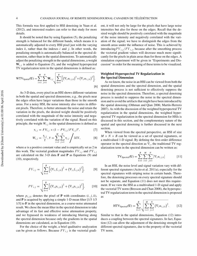
In the following, we present an example to help with theunderstanding of the complementary nature of the 2 regulariza-tion terms. In Figure 2, with the Washington DC Mall datasetas an example, the denoising results using models (18), (19),and (20) are presented, respectively. The data we used were thesame as the data used in “Experiments and Discussion,” andthe σ Equation (34) was set as 0.4. Note that for all the meth-ods, the regularization parameters were adjusted to achieve thehighest SNR. The first row represents the denoised band 100(1569.46 nm), the magnified local results in the red rectanglearea are shown in the second row, and the third row shows thespectral curves of pixel (153, 124). From the results shown inFigure 2, we can see that the noise in the spatial dimensions canbe effectively removed by the use of the model in (18), but thereis still noise in the spectral dimension. Conversely, the noise inthe spectral dimension can be effectively removed by the use ofthe model in (19), but there is still noise remaining in the spatialdimensions. However, by using the combined model in (20), notonly is the noise in each dimension effectively removed, but theoversmoothing problem in both the spatial dimensions and thespectral dimension is alleviated.

NUMERICAL SOLUTIONHSIs are much larger than gray images, so algorithms need

to be efficient. The proposed model in Equation (20) has 2 reg-ularization terms and is difficult to solve by the use of gradientmethods. Luckily, in recent years, the ADMM algorithm hasproved to be able to effectively and efficiently solve many con-strained and unconstrained problems in the image processing

Dow

nloa

ded

by [

Ghe

nt U

nive

rsity

] at

01:

00 0

6 A

pril

2016

6 CANADIAN JOURNAL OF REMOTE SENSING/JOURNAL CANADIEN DE TELEDETECTION

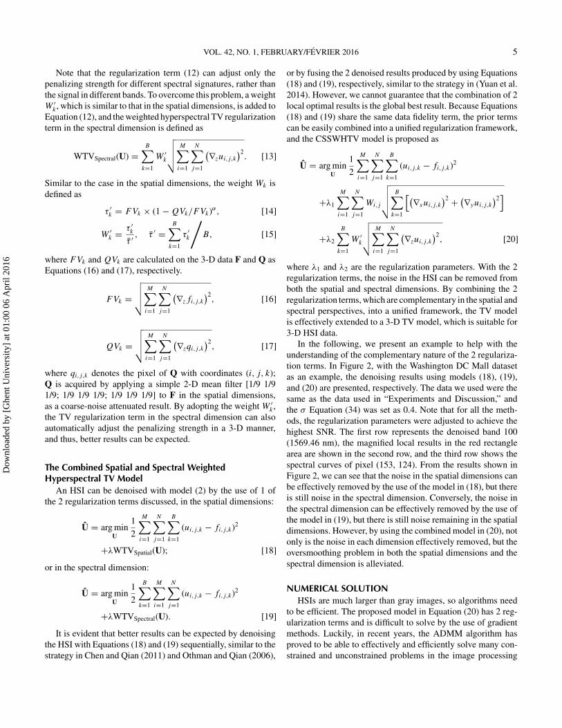
FIG. 2. Comparisons of the denoising results using different hyperspectral TV models. (a) The noisy data, (b) the result usingmodel (18), (c) the result using model (19), and (d) the result using model (20).

area, e.g., imaging inverse problems (Afonso et al. 2011) andunmixing (Bioucas-Dias and Figueiredo 2010; Iordache et al.2012, 2014; Zhao et al. 2013). In this section, we briefly reviewthe ADMM algorithm and then describe the version of ADMMused to solve the CSSWHTV model.

ADMM AlgorithmADMM benefits by decomposing a difficult problem into

a sequence of simple ones. The nature of ADMM is to usea variable splitting procedure followed by the adoption of anaugmented Lagrangian method. Consider the following uncon-strained problem:

minx

f1(x)+ f2(Gx) [21]

where x ∈ Rn, G ∈ Rp×n, f1 : Rn → R, and f2 : Rp → R.By creating a new variable,v ∈ Rn, Equation (21) is equivalentto:

minx,v

f1(x)+ f2(v), subject to v = Gx. [22]

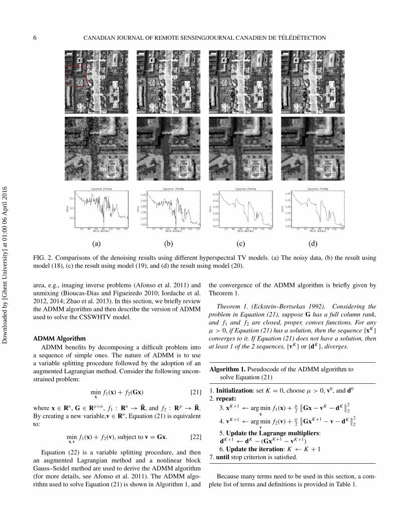
Equation (22) is a variable splitting procedure, and thenan augmented Lagrangian method and a nonlinear blockGauss–Seidel method are used to derive the ADMM algorithm(for more details, see Afonso et al. 2011). The ADMM algo-rithm used to solve Equation (21) is shown in Algorithm 1, and

the convergence of the ADMM algorithm is briefly given byTheorem 1.

Theorem 1. (Eckstein–Bertsekas 1992). Considering theproblem in Equation (21), suppose G has a full column rank,and f1 and f2 are closed, proper, convex functions. For anyμ > 0, if Equation (21) has a solution, then the sequence {xK}converges to it. If Equation (21) does not have a solution, thenat least 1 of the 2 sequences, {vK} or {dK}, diverges.

Algorithm 1. Pseudocode of the ADMM algorithm tosolve Equation (21)

1. Initialization: set K = 0, choose μ > 0, v0, and d0

2. repeat:3. xK+1 ← arg min

xf1(x)+ μ

2

∥∥Gx− vK − dK∥∥2

2

4. vK+1 ← arg minv

f2(v)+ μ

2

∥∥GxK+1 − v− dK∥∥2

2

5. Update the Lagrange multipliers:dK+1 ← dK − (GxK+1 − vK+1)6. Update the iteration: K ← K + 1

7. until stop criterion is satisfied.

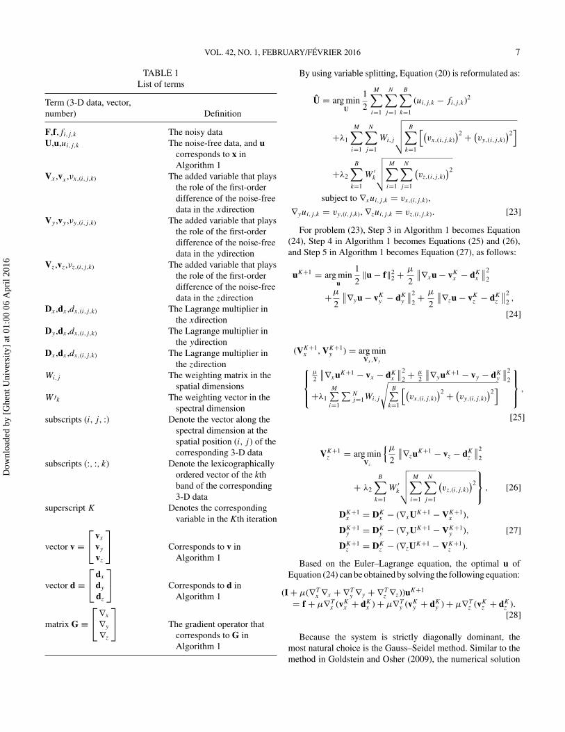
Because many terms need to be used in this section, a com-plete list of terms and definitions is provided in Table 1.

Dow

nloa

ded

by [

Ghe

nt U

nive

rsity

] at

01:

00 0

6 A

pril

2016

VOL. 42, NO. 1, FEBRUARY/FEVRIER 2016 7

TABLE 1List of terms

Term (3-D data, vector,number) Definition

F,f,fi,j,k The noisy dataU,u,ui,j,k The noise-free data, and u

corresponds to x inAlgorithm 1

Vx ,vx ,νx,(i,j,k) The added variable that playsthe role of the first-orderdifference of the noise-freedata in the xdirection

Vy ,vy ,νy,(i,j,k) The added variable that playsthe role of the first-orderdifference of the noise-freedata in the ydirection

Vz,vz,νz,(i,j,k) The added variable that playsthe role of the first-orderdifference of the noise-freedata in the zdirection

Dx ,dx ,dx,(i,j,k) The Lagrange multiplier inthe xdirection

Dy ,dx ,dx,(i,j,k) The Lagrange multiplier inthe ydirection

Dx ,dx ,dx,(i,j,k) The Lagrange multiplier inthe zdirection

Wi,j The weighting matrix in thespatial dimensions

W ′k The weighting vector in thespectral dimension

subscripts (i, j, :) Denote the vector along thespectral dimension at thespatial position (i, j ) of thecorresponding 3-D data

subscripts (:, :, k) Denote the lexicographicallyordered vector of the kthband of the corresponding3-D data

superscript K Denotes the correspondingvariable in the Kth iteration

vector v ≡⎡⎣vx

vy

vz

⎤⎦ Corresponds to v in

Algorithm 1

vector d ≡⎡⎣dx

dy

dz

⎤⎦ Corresponds to d in

Algorithm 1

matrix G ≡⎡⎣∇x

∇y

∇z

⎤⎦ The gradient operator that

corresponds to G inAlgorithm 1

By using variable splitting, Equation (20) is reformulated as:

U = arg minU

1

2

M∑i=1

N∑j=1

B∑k=1

(ui,j,k − fi,j,k)2

+λ1

M∑i=1

N∑j=1

Wi,j

√√√√ B∑k=1

[(vx,(i,j,k)

)2 + (vy,(i,j,k)

)2]

+λ2

B∑k=1

W ′k

√√√√ M∑i=1

N∑j=1

(vz,(i,j,k)

)2

subject to ∇xui,j,k = vx,(i,j,k),

∇yui,j,k = vy,(i,j,k),∇zui,j,k = vz,(i,j,k). [23]

For problem (23), Step 3 in Algorithm 1 becomes Equation(24), Step 4 in Algorithm 1 becomes Equations (25) and (26),and Step 5 in Algorithm 1 becomes Equation (27), as follows:

uK+1 = arg minu

1

2‖u− f‖2

2 +μ

2

∥∥∇xu− vKx − dK

x

∥∥2

2

+μ

2

∥∥∇yu− vKy − dK

y

∥∥2

2+ μ

2

∥∥∇zu− vKz − dK

z

∥∥2

2 ,

[24]

(VK+1x , VK+1

y ) = arg minVx ,Vy⎧⎪⎨

⎪⎩μ

2

∥∥∇xuK+1 − vx − dKx

∥∥22 + μ

2

∥∥∇yuK+1 − vy − dKy

∥∥2

2

+λ1

M∑i=1

∑Nj=1Wi,j

√B∑

k=1

[(vx,(i,j,k)

)2 + (vy,(i,j,k)

)2]

⎫⎪⎬⎪⎭ ,

[25]

VK+1z = arg min

Vz

{μ

2

∥∥∇zuK+1 − vz − dKz

∥∥2

2

+ λ2

B∑k=1

W ′k

√√√√ M∑i=1

N∑j=1

(vz,(i,j,k)

)2

⎫⎬⎭ , [26]

DK+1x = DK

x − (∇xUK+1 − VK+1x ),

DK+1y = DK

y − (∇yUK+1 − VK+1y ),

DK+1z = DK

z − (∇zUK+1 − VK+1z ).

[27]

Based on the Euler–Lagrange equation, the optimal u ofEquation (24) can be obtained by solving the following equation:

(I+ μ(∇Tx ∇x + ∇T

y ∇y + ∇Tz ∇z))uK+1

= f + μ∇Tx (vK

x + dKx )+ μ∇T

y (vKy + dK

y )+ μ∇Tz (vK

z + dKz ).[28]

Because the system is strictly diagonally dominant, themost natural choice is the Gauss–Seidel method. Similar to themethod in Goldstein and Osher (2009), the numerical solution

Dow

nloa

ded

by [

Ghe

nt U

nive

rsity

] at

01:

00 0

6 A

pril

2016

8 CANADIAN JOURNAL OF REMOTE SENSING/JOURNAL CANADIEN DE TELEDETECTION

to this problem can be written component-wise as

uK+1i,j,k =

μ

1+ 6μ(uK

i−1,j,k + uKi+1,j,k + uK

i,j−1,k

+uKi,j+1,k + uK

i,j,k−1 + uKi,j,k+1 + vK

x,(i−1,j,k)

−vKx,(i,j,k) + dK

x,(i−1,j,k) − dKx,(i,j,k) + vK

y,(i,j−1,k)

−vKy,(i,j,k) + dK

y,(i,j−1,k) − dKy,(i,j,k) + vK

z,(i,j,k−1)

−vKz,(i,j,k) + dK

z,(i,j,k−1) − dKz,(i,j,k))+

1

1+ 6μfi,j,k.

[29]

The solution Equations (25) and (26) can be obtained by thewell-known vect-soft threshold. For a vector a and threshold τ ,the vect-soft threshold is defined as:

vect-soft {a, τ } ={

max(‖a‖2 − τ, 0)

max(‖a‖2 − τ, 0)+ τ· a}

. [30]

Letting vx,(i,j, :), vy,(i,j, :), (∇xu− dx)(i,j, :), and (∇yu− dy)(i,j, :)

denote the vectors along the spectral direction at spatial position(i, j ) of Vx , Vy , (∇xU−Dx), and (∇yU−Dy), respectively, the

solution of Equation (25) is given by

[vK+1

x,(i,j, :)

vK+1y,(i,j, :)

]= vect-soft

⎧⎨⎩⎡⎣ (∇xuK+1 − dK

x )(i,j, :)

(∇yuK+1 − dKy )(i,j, :)

⎤⎦ ,

λ1Wi,j

μ

⎫⎬⎭ .

[31]Letting vz,( : , : ,k) and (∇zu − dz)( : , : ,k) denote the lexico-

graphically ordered column vectors of the kth band of Vz and(∇zU − Dz), respectively, the solution of Equation (26) is pre-sented as

vK+1z,( : , : ,k) = vect-soft

{(∇zuK+1 − dK

z )( : , : ,k),λ2W

′k

μ

}. [32]

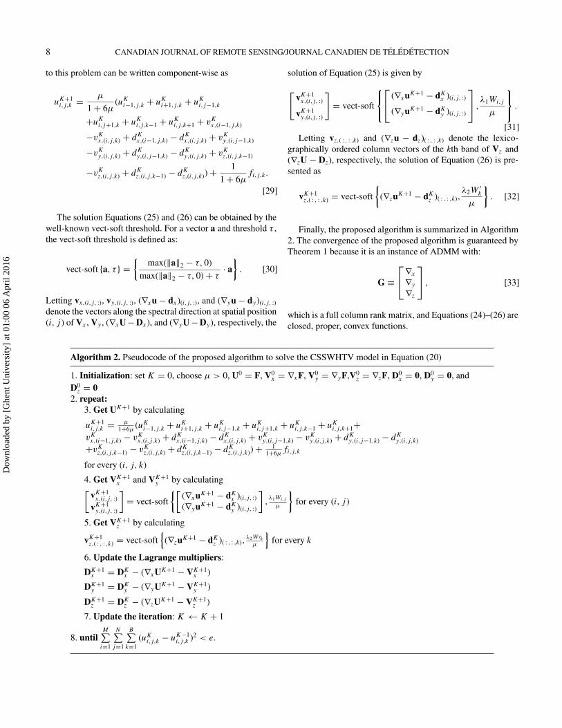
Finally, the proposed algorithm is summarized in Algorithm2. The convergence of the proposed algorithm is guaranteed byTheorem 1 because it is an instance of ADMM with:

G ≡⎡⎣∇x

∇y

∇z

⎤⎦ , [33]

which is a full column rank matrix, and Equations (24)–(26) areclosed, proper, convex functions.

Algorithm 2. Pseudocode of the proposed algorithm to solve the CSSWHTV model in Equation (20)

1. Initialization: set K = 0, choose μ > 0, U0 = F, V0x = ∇xF, V0

y = ∇yF,V0z = ∇zF, D0

x = 0, D0y = 0, and

D0z = 0

2. repeat:3. Get UK+1 by calculating

uK+1i,j,k = μ

1+6μ(uK

i−1,j,k + uKi+1,j,k + uK

i,j−1,k + uKi,j+1,k + uK

i,j,k−1 + uKi,j,k+1+

vKx,(i−1,j,k) − vK

x,(i,j,k) + dKx,(i−1,j,k) − dK

x,(i,j,k) + vKy,(i,j−1,k) − vK

y,(i,j,k) + dKy,(i,j−1,k) − dK

y,(i,j,k)

+vKz,(i,j,k−1) − vK

z,(i,j,k) + dKz,(i,j,k−1) − dK

z,(i,j,k))+ 11+6μ

fi,j,k

for every (i, j, k)

4. Get VK+1x and VK+1

y by calculating[vK+1

x,(i,j, :)

vK+1y,(i,j, :)

]= vect-soft

{[(∇xuK+1 − dK

x )(i,j, :)

(∇yuK+1 − dKy )(i,j, :)

],λ1Wi,j

μ

}for every (i, j )

5. Get VK+1z by calculating

vK+1z,( : , : ,k) = vect-soft

{(∇zuK+1 − dK

z )( : , : ,k),λ2W ′k

μ

}for every k

6. Update the Lagrange multipliers:

DK+1x = DK

x − (∇xUK+1 − VK+1x )

DK+1y = DK

y − (∇yUK+1 − VK+1y )

DK+1z = DK

z − (∇zUK+1 − VK+1z )

7. Update the iteration: K ← K + 1

8. untilM∑i=1

N∑j=1

B∑k=1

(uKi,j,k − uK−1

i,j,k )2 < e.

Dow

nloa

ded

by [

Ghe

nt U

nive

rsity

] at

01:

00 0

6 A

pril

2016

VOL. 42, NO. 1, FEBRUARY/FEVRIER 2016 9

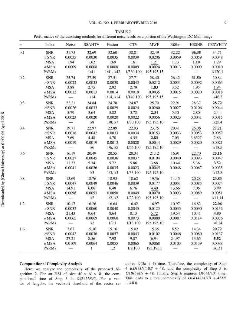
TABLE 2Performance of the denoising methods for different noise levels on a portion of the Washington DC Mall image

σ Index Noise SSAHTV Fusion CTV MWF BiShr. HSSNR CSSWHTV

0.1 SNR 31.75 32.69 32.60 32.81 32.49 32.22 36.35 34.71σSNR 0.0035 0.0030 0.0035 0.0039 0.0206 0.0059 0.0059 0.0048MSA 1.94 1.62 1.69 1.61 1.21 1.73 1.10 1.29σMSA 0.0009 0.0008 0.0008 0.0009 0.0024 0.0013 0.0009 0.0010PARMs — 1/41 1/41,1/42 1/360,100 195,195,15 — — 1/120,1

0.2 SNR 25.74 27.59 27.51 27.71 28.40 26.42 31.50 30.84σSNR 0.0022 0.0033 0.0030 0.0043 0.0212 0.0031 0.0092 0.0063MSA 3.88 2.75 2.92 2.79 1.83 3.52 1.95 1.94σMSA 0.0012 0.0013 0.0014 0.0019 0.0035 0.0015 0.0020 0.0018PARMs — 1/14 1/14,1/14 1/140,100 195,195,15 — — 1/46,2

0.3 SNR 22.21 24.84 24.78 24.87 25.70 22.91 28.37 28.72σSNR 0.0026 0.0033 0.0029 0.0024 0.0260 0.0027 0.0106 0.0044MSA 5.79 3.64 3.82 3.72 2.34 5.30 2.80 2.44σMSA 0.0023 0.0020 0.0020 0.0022 0.0056 0.0023 0.0041 0.0015PARMs — 1/8 1/8,1/7 1/80,100 195,195,10 — — 1/25,4

0.4 SNR 19.71 22.97 22.89 22.93 23.75 20.41 26.06 27.21σSNR 0.0018 0.0042 0.0033 0.0034 0.0153 0.0033 0.0053 0.0052MSA 7.69 4.48 4.70 4.55 2.83 7.05 3.6527 2.86σMSA 0.0019 0.0019 0.0013 0.0020 0.0044 0.0029 0.0020 0.0021PARMs — 1/6 1/6,1/5 1/56,100 195,195,10 — — 1/18,5

0.6 SNR 16.19 20.49 20.55 20.34 21.12 16.91 22.70 25.16σSNR 0.0027 0.0045 0.0036 0.0037 0.0104 0.0040 0.0093 0.0047MSA 11.37 5.34 5.72 5.86 3.68 10.44 5.36 3.52σMSA 0.0041 0.0026 0.0035 0.0023 0.0045 0.0048 0.0067 0.0035PARMs — 1/3 1/3,1/3 1/33,100 195,195,10 — — 1/12,8

0.8 SNR 13.69 18.76 18.95 18.62 19.36 14.45 20.28 23.83σSNR 0.0047 0.0049 0.0046 0.0039 0.0177 0.0051 0.0085 0.0074MSA 14.91 6.06 6.48 6.76 4.40 13.66 7.06 3.99σMSA 0.0098 0.0053 0.0050 0.0049 0.0070 0.0093 0.0089 0.0051PARMs — 1/2 1/2,1/2 1/22,100 195,195,10 — — 1/11,14

1.2 SNR 10.17 16.26 16.64 16.42 16.97 10.97 16.82 22.06σSNR 0.0032 0.0060 0.0040 0.0045 0.0125 0.0035 0.0090 0.0136MSA 21.43 9.64 8.64 8.13 5.72 19.54 10.41 4.80σMSA 0.0065 0.0069 0.0060 0.0073 0.0080 0.0087 0.0114 0.0076PARMs — 1/2 1/2,1 1/13,100 195,195,10 — — 1/8,24

1.6 SNR 7.67 15.36 15.16 15.02 15.35 8.52 14.34 20.72σSNR 0.0042 0.0036 0.0057 0.0043 0.0102 0.0046 0.0080 0.0137MSA 27.21 8.56 7.92 9.07 6.94 24.97 13.65 5.52σMSA 0.0109 0.0064 0.0055 0.0065 0.0068 0.0103 0.0139 0.0088PARMs — 1 1,2 1/9,100 195,195,5 — — 1/6,31

Computational Complexity AnalysisHere, we analyze the complexity of the proposed Al-

gorithm 2. For an HSI of size M × N × B, the com-putational time of Step 3 is O(21MNB ). For a vec-tor of lengthn, the vect-soft threshold of the vector re-

quires O(3n + 4) time. Therefore, the complexity of Step4 isO(MN (10B + 4)), and the complexity of Step 5 isO(B(5MN + 4)). Finally, Step 6 requires O(6MNB ) time.This leads to a total complexity of O(K(42MNB + 4MN+ 4B)).

Dow

nloa

ded

by [

Ghe

nt U

nive

rsity

] at

01:

00 0

6 A

pril

2016

10 CANADIAN JOURNAL OF REMOTE SENSING/JOURNAL CANADIEN DE TELEDETECTION

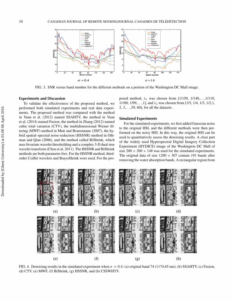
FIG. 3. SNR versus band number for the different methods on a portion of the Washington DC Mall image.

Experiments and DiscussionTo validate the effectiveness of the proposed method, we

performed both simulated experiments and real data experi-ments. The proposed method was compared with the methodin Yuan et al. (2012) named SSAHTV, the method in Yuanet al. (2014) named Fusion, the method in Zhang (2012) namedcubic total variation (CTV), the multidimensional Wiener fil-tering (MWF) method in Muti and Bourennane (2007), the hy-brid spatial–spectral noise-reduction (HSSNR) method in Oth-man and Qian (2006), and the method called BiShrink, whichuses bivariate wavelet thresholding and a complex 3-D dual-treewavelet transform (Chen et al. 2011). The HSSNR and BiShrinkmethods are both parameter free. For the HSSNR method, third-order Coiflet wavelets and BayesShrink were used. For the pro-

posed method, λ1 was chosen from [1/150, 1/140,. . .,1/110,1/100, 1/99,. . .,1], and λ2 was chosen from [1/5, 1/4, 1/3, 1/2,1,2, 3,. . .,59, 60], for all the datasets.

Simulated ExperimentsFor the simulated experiments, we first added Gaussian noise

to the original HSI, and the different methods were then per-formed on the noisy HSI. In this way, the original HSI can beused to quantitatively assess the denoising results. A clear partof the widely used Hyperspectral Digital Imagery CollectionExperiment (HYDICE) image of the Washington DC Mall ofsize 200× 200× 148 was used for the simulated experiments.The original data of size 1280 × 307 contain 191 bands afterremoving the water absorption bands. A rectangular region from

FIG. 4. Denoising results in the simulated experiment when σ = 0.4: (a) original band 74 (1174.65 nm), (b) SSAHTV, (c) Fusion,(d) CTV, (e) MWF, (f) BiShrink, (g) HSSNR, and (h) CSSWHTV.

Dow

nloa

ded

by [

Ghe

nt U

nive

rsity

] at

01:

00 0

6 A

pril

2016

VOL. 42, NO. 1, FEBRUARY/FEVRIER 2016 11

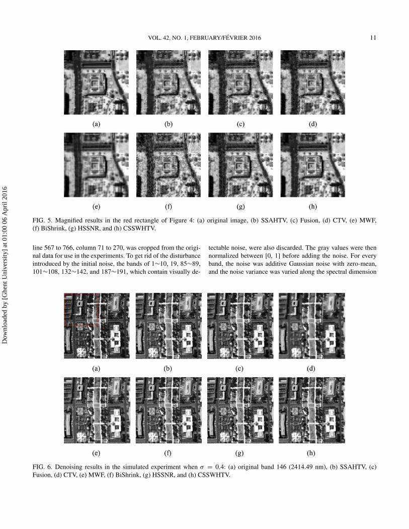
FIG. 5. Magnified results in the red rectangle of Figure 4: (a) original image, (b) SSAHTV, (c) Fusion, (d) CTV, (e) MWF,(f) BiShrink, (g) HSSNR, and (h) CSSWHTV.

line 567 to 766, column 71 to 270, was cropped from the origi-nal data for use in the experiments. To get rid of the disturbanceintroduced by the initial noise, the bands of 1∼10, 19, 85∼89,101∼108, 132∼142, and 187∼191, which contain visually de-

tectable noise, were also discarded. The gray values were thennormalized between [0, 1] before adding the noise. For everyband, the noise was additive Gaussian noise with zero-mean,and the noise variance was varied along the spectral dimension

FIG. 6. Denoising results in the simulated experiment when σ = 0.4: (a) original band 146 (2414.49 nm), (b) SSAHTV, (c)Fusion, (d) CTV, (e) MWF, (f) BiShrink, (g) HSSNR, and (h) CSSWHTV.

Dow

nloa

ded

by [

Ghe

nt U

nive

rsity

] at

01:

00 0

6 A

pril

2016

12 CANADIAN JOURNAL OF REMOTE SENSING/JOURNAL CANADIEN DE TELEDETECTION

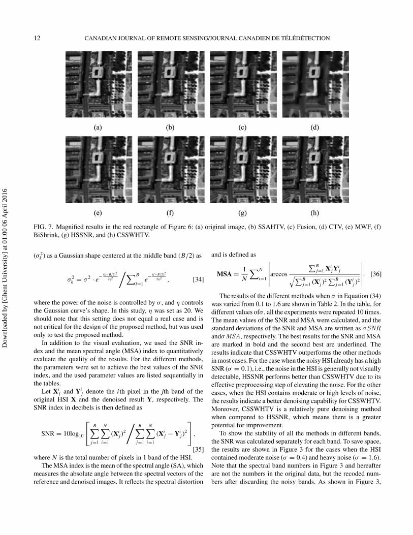
FIG. 7. Magnified results in the red rectangle of Figure 6: (a) original image, (b) SSAHTV, (c) Fusion, (d) CTV, (e) MWF, (f)BiShrink, (g) HSSNR, and (h) CSSWHTV.

(σ 2k ) as a Gaussian shape centered at the middle band (B/2) as

σ 2k = σ 2 · e−

(k−B/2)2

2η2

/∑B

l=1e− (l−B/2)2

2η2 , [34]

where the power of the noise is controlled by σ , and η controlsthe Gaussian curve’s shape. In this study, η was set as 20. Weshould note that this setting does not equal a real case and isnot critical for the design of the proposed method, but was usedonly to test the proposed method.

In addition to the visual evaluation, we used the SNR in-dex and the mean spectral angle (MSA) index to quantitativelyevaluate the quality of the results. For the different methods,the parameters were set to achieve the best values of the SNRindex, and the used parameter values are listed sequentially inthe tables.

Let Xij and Yi

j denote the ith pixel in the jth band of theoriginal HSI X and the denoised result Y, respectively. TheSNR index in decibels is then defined as

SNR = 10log10

⎡⎣ B∑

j=1

N∑i=1

(Xij )2

/B∑

j=1

N∑i=1

(Xij − Yi

j )2

⎤⎦ ,

[35]where N is the total number of pixels in 1 band of the HSI.

The MSA index is the mean of the spectral angle (SA), whichmeasures the absolute angle between the spectral vectors of thereference and denoised images. It reflects the spectral distortion

and is defined as

MSA = 1

N

∑N

i=1

∣∣∣∣∣∣arccos

∑Bj=1 Xi

j Yij√∑B

j=1 (Xij )2

∑Bj=1 (Yi

j )2

∣∣∣∣∣∣. [36]

The results of the different methods when σ in Equation (34)was varied from 0.1 to 1.6 are shown in Table 2. In the table, fordifferent values ofσ , all the experiments were repeated 10 times.The mean values of the SNR and MSA were calculated, and thestandard deviations of the SNR and MSA are written as σSNRandσMSA, respectively. The best results for the SNR and MSAare marked in bold and the second best are underlined. Theresults indicate that CSSWHTV outperforms the other methodsin most cases. For the case when the noisy HSI already has a highSNR (σ = 0.1), i.e., the noise in the HSI is generally not visuallydetectable, HSSNR performs better than CSSWHTV due to itseffective preprocessing step of elevating the noise. For the othercases, when the HSI contains moderate or high levels of noise,the results indicate a better denoising capability for CSSWHTV.Moreover, CSSWHTV is a relatively pure denoising methodwhen compared to HSSNR, which means there is a greaterpotential for improvement.

To show the stability of all the methods in different bands,the SNR was calculated separately for each band. To save space,the results are shown in Figure 3 for the cases when the HSIcontained moderate noise (σ = 0.4) and heavy noise (σ = 1.6).Note that the spectral band numbers in Figure 3 and hereafterare not the numbers in the original data, but the recoded num-bers after discarding the noisy bands. As shown in Figure 3,

Dow

nloa

ded

by [

Ghe

nt U

nive

rsity

] at

01:

00 0

6 A

pril

2016

VOL. 42, NO. 1, FEBRUARY/FEVRIER 2016 13

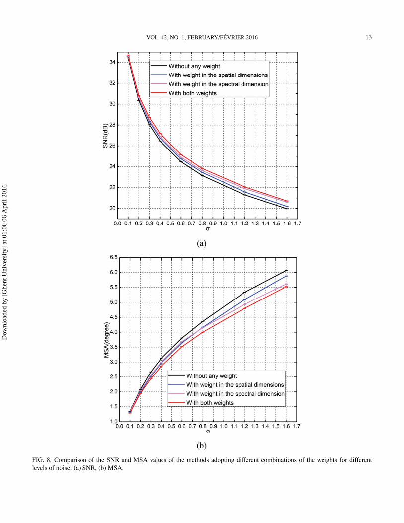
FIG. 8. Comparison of the SNR and MSA values of the methods adopting different combinations of the weights for differentlevels of noise: (a) SNR, (b) MSA.

Dow

nloa

ded

by [

Ghe

nt U

nive

rsity

] at

01:

00 0

6 A

pril

2016

14 CANADIAN JOURNAL OF REMOTE SENSING/JOURNAL CANADIEN DE TELEDETECTION

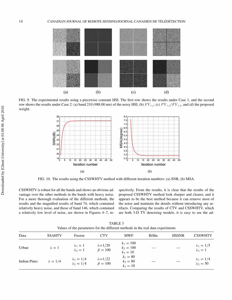
FIG. 9. The experimental results using a piecewise constant HSI. The first row shows the results under Case 1, and the secondrow shows the results under Case 2: (a) band 210 (988.00 nm) of the noisy HSI, (b) FV i,j , (c) PV i,j /FV i,j , and (d) the proposedweight.

FIG. 10. The results using the CSSWHTV method with different iteration numbers: (a) SNR, (b) MSA.

CSSWHTV is robust for all the bands and shows an obvious ad-vantage over the other methods in the bands with heavy noise.For a more thorough evaluation of the different methods, theresults and the magnified results of band 74, which containedrelatively heavy noise, and those of band 146, which containeda relatively low level of noise, are shown in Figures 4–7, re-

spectively. From the results, it is clear that the results of theproposed CSSWHTV method look sharper and clearer, and itappears to be the best method because it can remove most ofthe noise and maintain the details without introducing any ar-tifacts. Comparing the results of CTV and CSSWHTV, whichare both 3-D TV denoising models, it is easy to see the ad-

TABLE 3Values of the parameters for the different methods in the real data experiments

Data SSAHTV Fusion CTV MWF BiShr. HSSNR CSSWHTV

Urban λ = 1λ1 = 1λ2 = 1

λ=1/20β = 100

k1 = 100k2 = 100k3 = 10

— —λ1 = 1/5λ2 = 1

Indian Pines λ = 1/4λ1 = 1/4λ2 = 1/4

λ=1/22β = 100

k1 = 80k2 = 80k3 = 10

— —λ1 = 1/4λ2 = 50

Dow

nloa

ded

by [

Ghe

nt U

nive

rsity

] at

01:

00 0

6 A

pril

2016

VOL. 42, NO. 1, FEBRUARY/FEVRIER 2016 15

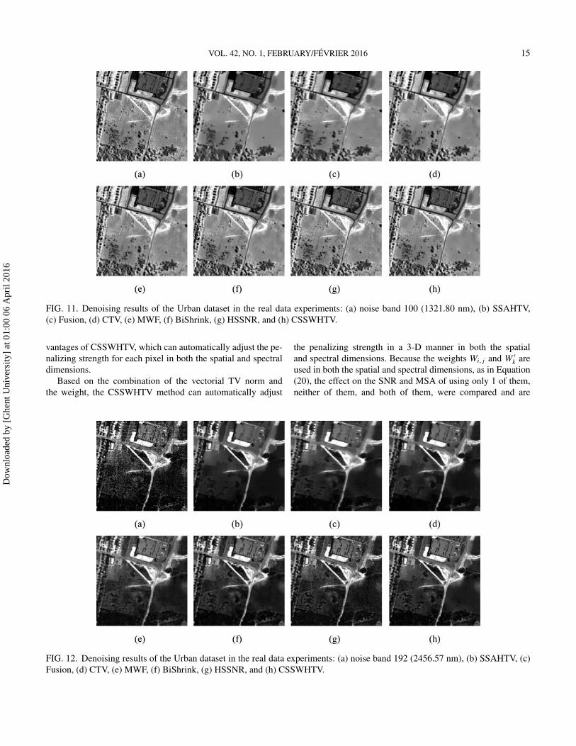
FIG. 11. Denoising results of the Urban dataset in the real data experiments: (a) noise band 100 (1321.80 nm), (b) SSAHTV,(c) Fusion, (d) CTV, (e) MWF, (f) BiShrink, (g) HSSNR, and (h) CSSWHTV.

vantages of CSSWHTV, which can automatically adjust the pe-nalizing strength for each pixel in both the spatial and spectraldimensions.

Based on the combination of the vectorial TV norm andthe weight, the CSSWHTV method can automatically adjust

the penalizing strength in a 3-D manner in both the spatialand spectral dimensions. Because the weights Wi,j and W ′k areused in both the spatial and spectral dimensions, as in Equation(20), the effect on the SNR and MSA of using only 1 of them,neither of them, and both of them, were compared and are

FIG. 12. Denoising results of the Urban dataset in the real data experiments: (a) noise band 192 (2456.57 nm), (b) SSAHTV, (c)Fusion, (d) CTV, (e) MWF, (f) BiShrink, (g) HSSNR, and (h) CSSWHTV.

Dow

nloa

ded

by [

Ghe

nt U

nive

rsity

] at

01:

00 0

6 A

pril

2016

16 CANADIAN JOURNAL OF REMOTE SENSING/JOURNAL CANADIEN DE TELEDETECTION

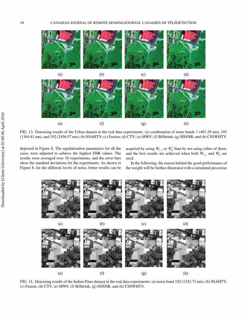
FIG. 13. Denoising results of the Urban dataset in the real data experiments: (a) combination of noise bands 1 (401.29 nm), 103(1364.81 nm), and 192 (2456.57 nm); (b) SSAHTV; (c) Fusion; (d) CTV; (e) MWF; (f) BiShrink; (g) HSSNR; and (h) CSSWHTV.

depicted in Figure 8. The regularization parameters for all thecases were adjusted to achieve the highest SNR values. Theresults were averaged over 10 experiments, and the error barsshow the standard deviations for the experiments. As shown inFigure 8, for the different levels of noise, better results can be

acquired by using Wi,j or W ′k than by not using either of them,and the best results are achieved when both Wi,j and W ′k areused.

In the following, the reason behind the good performance ofthe weight will be further illustrated with a simulated piecewise

FIG. 14. Denoising results of the Indian Pines dataset in the real data experiments: (a) noise band 102 (1342.73 nm), (b) SSAHTV,(c) Fusion, (d) CTV, (e) MWF, (f) BiShrink, (g) HSSNR, and (h) CSSWHTV.

Dow

nloa

ded

by [

Ghe

nt U

nive

rsity

] at

01:

00 0

6 A

pril

2016

VOL. 42, NO. 1, FEBRUARY/FEVRIER 2016 17

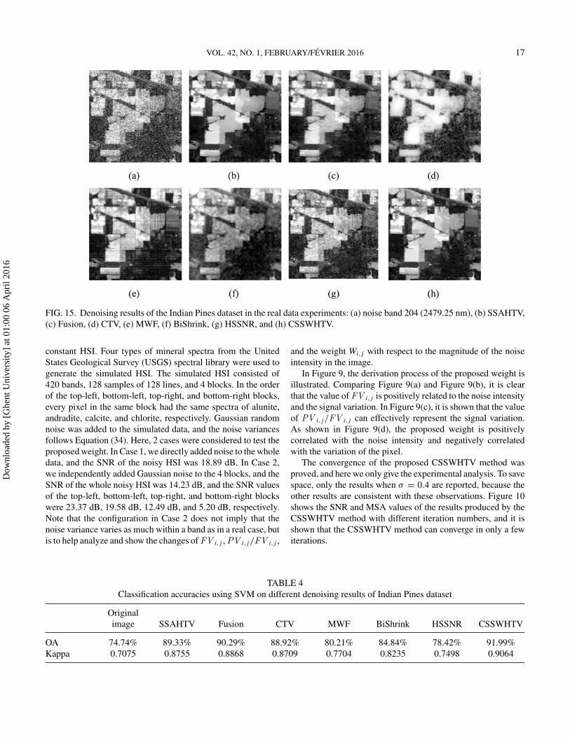
FIG. 15. Denoising results of the Indian Pines dataset in the real data experiments: (a) noise band 204 (2479.25 nm), (b) SSAHTV,(c) Fusion, (d) CTV, (e) MWF, (f) BiShrink, (g) HSSNR, and (h) CSSWHTV.

constant HSI. Four types of mineral spectra from the UnitedStates Geological Survey (USGS) spectral library were used togenerate the simulated HSI. The simulated HSI consisted of420 bands, 128 samples of 128 lines, and 4 blocks. In the orderof the top-left, bottom-left, top-right, and bottom-right blocks,every pixel in the same block had the same spectra of alunite,andradite, calcite, and chlorite, respectively. Gaussian randomnoise was added to the simulated data, and the noise variancesfollows Equation (34). Here, 2 cases were considered to test theproposed weight. In Case 1, we directly added noise to the wholedata, and the SNR of the noisy HSI was 18.89 dB. In Case 2,we independently added Gaussian noise to the 4 blocks, and theSNR of the whole noisy HSI was 14.23 dB, and the SNR valuesof the top-left, bottom-left, top-right, and bottom-right blockswere 23.37 dB, 19.58 dB, 12.49 dB, and 5.20 dB, respectively.Note that the configuration in Case 2 does not imply that thenoise variance varies as much within a band as in a real case, butis to help analyze and show the changes of FV i,j , PV i,j /FV i,j ,

and the weight Wi,j with respect to the magnitude of the noiseintensity in the image.

In Figure 9, the derivation process of the proposed weight isillustrated. Comparing Figure 9(a) and Figure 9(b), it is clearthat the value of FV i,j is positively related to the noise intensityand the signal variation. In Figure 9(c), it is shown that the valueof PV i,j /FV i,j can effectively represent the signal variation.As shown in Figure 9(d), the proposed weight is positivelycorrelated with the noise intensity and negatively correlatedwith the variation of the pixel.

The convergence of the proposed CSSWHTV method wasproved, and here we only give the experimental analysis. To savespace, only the results when σ = 0.4 are reported, because theother results are consistent with these observations. Figure 10shows the SNR and MSA values of the results produced by theCSSWHTV method with different iteration numbers, and it isshown that the CSSWHTV method can converge in only a fewiterations.

TABLE 4Classification accuracies using SVM on different denoising results of Indian Pines dataset

Originalimage SSAHTV Fusion CTV MWF BiShrink HSSNR CSSWHTV

OA 74.74% 89.33% 90.29% 88.92% 80.21% 84.84% 78.42% 91.99%Kappa 0.7075 0.8755 0.8868 0.8709 0.7704 0.8235 0.7498 0.9064

Dow

nloa

ded

by [

Ghe

nt U

nive

rsity

] at

01:

00 0

6 A

pril

2016

18 CANADIAN JOURNAL OF REMOTE SENSING/JOURNAL CANADIEN DE TELEDETECTION

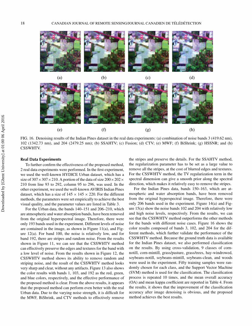
FIG. 16. Denoising results of the Indian Pines dataset in the real data experiments: (a) combination of noise bands 3 (419.62 nm),102 (1342.73 nm), and 204 (2479.25 nm); (b) SSAHTV; (c) Fusion; (d) CTV; (e) MWF; (f) BiShrink; (g) HSSNR; and (h)CSSWHTV.

Real Data ExperimentsTo further confirm the effectiveness of the proposed method,

2 real data experiments were performed. In the first experiment,we used the well-known HYDICE Urban dataset, which has asize of 307×307×210. A portion of the data of size 200×202×210 from line 93 to 292, column 95 to 296, was used. In theother experiment, we used the well-known AVIRIS Indian Pinesdataset, which has a size of 145× 145× 220. For the differentmethods, the parameters were set empirically to achieve the bestvisual quality, and the parameter values are listed in Table 3.

For the Urban data, the bands 140–151 and 206–210, whichare atmospheric and water absorption bands, have been removedfrom the original hyperspectral image. Therefore, there wereonly 193 bands used in the experiment. Different levels of noiseare contained in the image, as shown in Figure 11(a), and Fig-ure 12(a). For band 100, the noise is relatively low, and forband 192, there are stripes and random noise. From the resultsshown in Figure 11, we can see that the CSSWHTV methodcan effectively preserve the edges and textures for the band witha low level of noise. From the results shown in Figure 12, theCSSWHTV method shows its ability to remove random andstriping noise, and the result of the CSSWHTV method looksvery sharp and clear, without any artifacts. Figure 13 also showsthe color results with bands 1, 103, and 192 as the red, green,and blue colors, respectively, and the effective performance ofthe proposed method is clear. From the above results, it appearsthat the proposed method can perform even better with the realUrban data. Due to the varying noise strength, it is difficult forthe MWF, BiShrink, and CTV methods to effectively remove

the stripes and preserve the details. For the SSAHTV method,the regularization parameter has to be set as a large value toremove all the stripes, at the cost of blurred edges and textures.For the CSSWHTV method, the TV regularization term in thespectral dimension can give a smooth prior along the spectraldirection, which makes it relatively easy to remove the stripes.

For the Indian Pines data, bands 150–163, which are at-mospheric and water absorption bands, have been removedfrom the original hyperspectral image. Therefore, there wereonly 206 bands used in the experiment. Figure 14(a) and Fig-ure 15(a) show the noise bands 102 and 204 with relatively lowand high noise levels, respectively. From the results, we cansee that the CSSWHTV method outperforms the other methodsfor the bands with different noise cases. Figure 16 shows thecolor results composed of bands 3, 102, and 204 for the dif-ferent methods, which further validate the performance of theCSSWHTV method. Because the ground truth data is availablefor the Indian Pines dataset, we also performed classificationon the results. By using cross-validation, 9 classes of corn-notill, corn-mintill, grass/pasture, grass/trees, hay-windrowed,soybeans-notill, soybeans-mintill, soybeans-clean, and woodswere used in the experiment. Fifty training samples were ran-domly chosen for each class, and the Support Vector Machine(SVM) method is used for the classification. The classificationprocess is repeated 10 times, and the mean overall accuracy(OA) and mean kappa coefficient are reported in Table 4. Fromthe results, it shows that the improvement of the classificationaccuracy after image denoising is obvious, and the proposedmethod achieves the best results.

Dow

nloa

ded

by [

Ghe

nt U

nive

rsity

] at

01:

00 0

6 A

pril

2016

VOL. 42, NO. 1, FEBRUARY/FEVRIER 2016 19

CONCLUSIONSIn this article, a combined spatial and spectral weighted hy-

perspectral total variation (CSSWHTV) model has been pro-posed for denoising HSIs. By viewing the HSI as a 3-D cube, thenew model combines the TV regularizations in both the spatialand spectral dimensions into a unified framework. Moreover, toclearly remove the noise and retain the edges, the regularizationterms have been designed to be able to automatically controlthe penalizing strength for each pixel in both the spatial andspectral dimensions. To solve the proposed new model, we haveproposed a new algorithm, which is a version of the well-knownADMM procedure, which is fast and has a good convergenceproperty. Both simulated and real data experiments were con-ducted to validate the effectiveness of the proposed method.The consistent improvements when compared with the otherwell-known methods in different noise cases show that the pro-posed method is robust and can effectively remove noise whilepreserving the details, without introducing any new artifacts.

Despite the effective performance of the proposed method,an investigation into what extent it could improve the precisionof the subsequent applications would be interesting. The au-tomatic and efficient selection of the regularization parametersalso needs further study.

FUNDINGThis work was supported in part by the 863 program under

Grant 2013AA12A301, by the National Natural Science Foun-dation of China under Grants 41571362 and 41431175, and bythe NASG Key Laboratory of Land Environment and DisasterMonitoring (No. LEDM2014B01).

REFERENCESAcito, N., Diani, M., and Corsini, G. 2010. “Hyperspectral signal sub-

space identification in the presence of rare signal components.” IEEETransactions on Geoscience and Remote Sensing, Vol. 48(No. 4): pp.1940–1954.

Acito, N., Diani, M., and Corsini, G. 2011a. “Signal-dependent noisemodeling and model parameter estimation in hyperspectral images.”IEEE Transactions on Geoscience and Remote Sensing, Vol. 49(No.8): pp. 2957–2971.

Acito, N., Diani, M., and Corsini, G. 2011b. “Subspace-based strip-ing noise reduction in hyperspectral images.” IEEE Transactions onGeoscience and Remote Sensing, Vol. 49(No. 4): pp. 1325–1342.

Afonso, M. V., Bioucas-Dias, J. M., and Figueiredo, M. A. 2011. “Anaugmented Lagrangian approach to the constrained optimization for-mulation of imaging inverse problems.” IEEE Transactions on ImageProcessing, Vol. 20(No. 3): pp. 681–695.

Alparone, L., Selva, M., Aiazzi, B., Baronti, S., Butera, F., and Chiaran-tini, L. 2009. “Signal-dependent noise modelling and estimation ofnew-generation imaging spectrometers.” Paper presented at IEEE 1stWorkshop on Hyperspectral Image & Signal Processing: Evolutionin Remote Sensing (WHISPERS), Grenoble, France, August 2009.

Bioucas-Dias, J. M., and Figueiredo, M. A. 2010. “Alternating direc-tion algorithms for constrained sparse regression: Application tohyperspectral unmixing.” Paper presented at IEEE 2nd Workshop

on Hyperspectral Image & Signal Processing: Evolution in RemoteSensing (WHISPERS), Reykjavik, Iceland, June 2010.

Bioucas-Dias, J. M., Figueiredo, M. A., and Oliveira, J. P. 2006. “Totalvariation-based image deconvolution: a majorization-minimizationapproach.” Paper presented at International Conference on Acous-tics, Speech and Signal Processing (ICASSP), Toulouse, France,May 2006.

Bresson, X., and Chan, T. F. 2008. “Fast dual minimization of the vecto-rial total variation norm and applications to color image processing.”Inverse Problems and Imaging, Vol. 2(No. 4): pp. 455–484.

Buades, A., Coll, B., and Morel, J.-M. 2005. “A non-local algorithmfor image denoising.” Paper presented at IEEE Computer Vision andPattern Recognition, San Diego, CA, June 2005.

Chen, G., Bui, T. D., and Krzyzak, A. 2011. “Denoising of three-dimensional data cube using bivariate wavelet shrinking.” Interna-tional Journal of Pattern Recognition and Artificial Intelligence, Vol.25(No. 3): pp. 403–413.

Chen, G., Bui, T. D., Quach, K. G., and Qian, S.-E. 2014. “Denois-ing hyperspectral imagery using principal component analysis andblock-matching 4D filtering.” Canadian Journal of Remote Sensing,Vol. 40(No. 1): pp. 60–66.

Chen, G., and Qian, S.-E. 2011. “Denoising of hyperspectral imageryusing principal component analysis and wavelet shrinkage.” IEEETransactions on Geoscience and Remote Sensing, Vol. 49(No. 3):pp. 973–980.

Chen, G., Qian, S.-E., and Gleason, S. 2012. “Denoising of hyperspec-tral imagery by combining PCA with block-matching 3-D filtering.”Canadian Journal of Remote Sensing, Vol. 37(No. 6): pp. 590–595.

Eckstein, J., and Bertsekas, D. P. 1992. “On the Douglas–Rachfordsplitting method and the proximal point algorithm for maximalmonotone operators.” Mathematical Programming, Vol. 55(No. 1-3): pp. 293–318.

Elad, M., and Aharon, M. 2006. “Image denoising via sparse and redun-dant representations over learned dictionaries.” IEEE Transactionson Image Processing, Vol. 15(No. 12): pp. 3736–3745.

Gabay, D., and Mercier, B. 1976. “A dual algorithm for the solutionof nonlinear variational problems via finite element approximation.”Computers & Mathematics with Applications, Vol. 2(No. 1): pp.17–40.

Goldstein, T., and Osher, S. 2009. “The split Bregman method forL1-regularized problems.” SIAM Journal on Imaging Sciences, Vol.2(No. 2): pp. 323–343.

Guo, X., Huang, X., Zhang, L., and Zhang, L. 2013. “Hyperspectralimage noise reduction based on rank-1 tensor decomposition.” ISPRSJournal of Photogrammetry and Remote Sensing, Vol. 83(No. 9): pp.50–63.

Harris, J., Ponomarev, P., Shang, J., and Rogge, D. 2006. “Noise reduc-tion and best band selection techniques for improving classificationresults using hyperspectral data: application to lithological map-ping in Canada’s Arctic.” Canadian Journal of Remote Sensing, Vol.32(No. 5): pp. 341–354.

He, W., Zhang, H., Zhang, L., and Shen, H. 2016. “ Total-variation-regularized low-rank matrix factorization for hyperspectral imagerestoration.” IEEE Transactions on Geoscience and Remote Sensing,Vol. 54(No. 1): pp. 178–188.

Iordache, M.-D., Bioucas-Dias, J. M., and Plaza, A. 2012. “Total varia-tion spatial regularization for sparse hyperspectral unmixing.” IEEETransactions on Geoscience and Remote Sensing, Vol. 50(No. 11):pp. 4484–4502.

Dow

nloa

ded

by [

Ghe

nt U

nive

rsity

] at

01:

00 0

6 A

pril

2016

20 CANADIAN JOURNAL OF REMOTE SENSING/JOURNAL CANADIEN DE TELEDETECTION

Iordache, M.-D., Bioucas-Dias, J. M., and Plaza, A. 2014. “Collabo-rative sparse regression for hyperspectral unmixing.” IEEE Trans-actions on Geoscience and Remote Sensing, Vol. 52(No. 1): pp.341–354.

Jiang, C., Zhang, H., Shen, H., and Zhang, L. 2014. “Two-step sparsecoding for the pan-sharpening of remote sensing images.” IEEE Jour-nal of Selected Topics in Applied Earth Observations and RemoteSensing, Vol. 7(No. 5): pp. 1792–1805.

Kuybeda, O., Malah, D., and Barzohar, M. 2007. “Rank estimation andredundancy reduction of high-dimensional noisy signals with preser-vation of rare vectors.” IEEE Transactions on Signal Processing, Vol.55(No. 12): pp. 5579–5592.

Letexier, D., and Bourennane, S. 2008. “Noise removal from hyper-spectral images by multidimensional filtering.” IEEE Transactionson Geoscience and Remote Sensing, Vol. 46(No. 7): pp. 2061–2069.

Li, T., Chen, X.-M., Xue, B., Li, Q.-Q., and Ni, G.-Q. 2010. “A totalvariation denoising algorithm for hyperspectral data.” Paper pre-sented at Photonics Asia, Beijing, China, October 2010.

Lin, T., and Bourennane, S. 2013a. “Hyperspectral image processingby jointly filtering wavelet component tensor.” IEEE Transactionson Geoscience and Remote Sensing, Vol. 51(No. 6): pp. 3529–3541.

Lin, T., and Bourennane, S. 2013b. “Survey of hyperspectral image de-noising methods based on tensor decompositions.” EURASIP Jour-nal on Advances in Signal Processing, Vol. 2013(No. 1): pp. 1–11.

Liu, X., Bourennane, S., and Fossati, C. 2012. “Denoising of hyperspec-tral images using the PARAFAC model and statistical performanceanalysis.” IEEE Transactions on Geoscience and Remote Sensing,Vol. 50(No. 10): pp. 3717–3724.

Mendez-Rial, R., Calvino-Cancela, M., and Martın-Herrero, J. 2010.“Accurate implementation of anisotropic diffusion in the hypercube.”IEEE Geoscience and Remote Sensing Letters, Vol. 7(No. 4): pp.870–874.

Maggioni, M., Katkovnik, V., Egiazarian, K., and Foi, A. 2013. “Non-local transform-domain filter for volumetric data denoising and re-construction.” IEEE Transactions on Image Processing, Vol. 22(No.1): pp. 119–133.

Martın-Herrero, J. 2007. “Anisotropic diffusion in the hypercube.”IEEE Transactions on Geoscience and Remote Sensing, Vol. 45(No.5): pp. 1386–1398.

Mendez-Rial, R., and Martin-Herrero, J. 2012. “Efficiency of semi-implicit schemes for anisotropic diffusion in the hypercube.” IEEETransactions on Image Processing, Vol. 21(No. 5): pp. 2389–2398.

Muti, D., and Bourennane, S. 2007. “Survey on tensor signal algebraicfiltering.” Signal Processing, Vol. 87(No. 2): pp. 237–249.

Othman, H., and Qian, S.-E. 2006. “Noise reduction of hyperspec-tral imagery using hybrid spatial-spectral derivative-domain waveletshrinkage.” IEEE Transactions on Geoscience and Remote Sensing,Vol. 44(No. 2): pp. 397–408.

Perona, P., and Malik, J. 1990. “Scale-space and edge detection usinganisotropic diffusion.” IEEE Transactions on Pattern Analysis andMachine Intelligence, Vol. 12(No. 7): pp. 629–639.

Portilla, J., Strela, V., Wainwright, M. J., and Simoncelli, E. P. 2003.“Image denoising using scale mixtures of Gaussians in the waveletdomain.” IEEE Transactions on Image Processing, Vol. 12(No. 11):pp. 1338–1351.

Qian, Y., Shen, Y., Ye, M., and Wang, Q. 2012. “3-D nonlocal meansfilter with noise estimation for hyperspectral imagery denoising.” Pa-per presented at IEEE International Geoscience and Remote SensingSymposium (IGARSS), Munich, Germany, July 2012.

Qian, Y., and Ye, M. 2013. “Hyperspectral imagery restoration us-ing nonlocal spectral-spatial structured sparse representation withnoise estimation.” IEEE Journal of Selected Topics in AppliedEarth Observations and Remote Sensing Vol. 6(No. 2): pp. 499–515.

Rasti, B., Sveinsson, J. R., and Ulfarsson, M. O. 2014. “Wavelet-basedsparse reduced-rank regression for hyperspectral image restoration.”IEEE Transactions on Geoscience and Remote Sensing, Vol. 52(No.10): pp. 6688–6698.

Rudin, L. I., Osher, S., and Fatemi, E. 1992. “Nonlinear total variationbased noise removal algorithms.” Physica D: Nonlinear Phenomena,Vol. 60(No. 1): pp. 259–268.

Selesnick, I. W. 2002. “Bivariate shrinkage functions for wavelet-baseddenoising exploiting interscale dependency.” IEEE Transactions onSignal Processing, Vol. 50(No. 11): pp. 2744–2756.

Sendur, L., and Selesnick, I. W. 2002. “Bivariate shrinkage with localvariance estimation.” IEEE Signal Processing Letters, Vol. 9(No.12): pp. 438–441.

Wang, Y., Niu, R., and Yu, X. 2010. “Anisotropic diffusion for hyper-spectral imagery enhancement.” IEEE Sensors Journal, Vol. 10(No.3): pp. 469–477.

Yang, J., Yin, W., Zhang, Y., and Wang, Y. 2009. “A fast algorithm foredge-preserving variational multichannel image restoration.” SIAMJournal on Imaging Sciences, Vol. 2(No. 2): pp. 569–592.

Yuan, Q., Zhang, L., and Shen, H. 2012. “Hyperspectral image denois-ing employing a spectral–spatial adaptive total variation model.”IEEE Transactions on Geoscience and Remote Sensing, Vol. 50(No.10): pp. 3660–3677.

Yuan, Q., Zhang, L., and Shen, H. 2014. “Hyperspectral image de-noising with a spatial–spectral view fusion strategy.” IEEE Transac-tions on Geoscience and Remote Sensing, Vol. 52(No. 5): pp. 2314–2325.

Zelinski, A. C., and Goyal, V. K. 2006. “Denoising hyperspectral im-agery and recovering junk bands using wavelets and sparse approx-imation.” Paper presented at IEEE International Geoscience andRemote Sensing Symposium (IGARSS), Denver, Colorado, USA,August 2006.

Zhang, H. 2012. “Hyperspectral image denoising with cubic total vari-ation model.” Paper presented at ISPRS Annals of Photogrammetry,Remote Sensing and Spatial Information Sciences, Melbourne, Aus-tralia, August 2012.

Zhang, H., He, W., Zhang, L., Shen, H., and Yuan, Q. 2014. “Hyper-spectral image restoration using low-rank matrix recovery.” IEEETransactions on Geoscience and Remote Sensing, Vol. 52(No. 8):pp. 4729–4743.

Zhang, H., Zhang, L., and Shen, H. 2012. “A super-resolution recon-struction algorithm for hyperspectral images.” Signal Processing,Vol. 92(No. 9): pp. 2082–2096.

Zhang, H., Zhai, H., Zhang, L., and Li, P. 2016. “Spectral-SpatialSparse Subspace Clustering for Hyperspectral Remote Sensing Im-ages.” IEEE Transactions on Geoscience and Remote Sensing, doi:10.1109/TGRS.2016.2524557.

Zhao, X.-L., Wang, F., Huang, T.-Z., Ng, M. K., and Plemmons, R. J.2013. “Deblurring and sparse unmixing for hyperspectral images.”IEEE Transactions on Geoscience and Remote Sensing, Vol. 51(No.7): pp. 4045–4058.

Zhao, Y.-Q., and Yang, J. 2015. “Hyperspectral image denoising viasparse representation and low-rank constraint.” IEEE Transactionson Geoscience and Remote Sensing, Vol. 53(No. 1): pp. 296–308.

Dow

nloa

ded

by [

Ghe

nt U

nive

rsity

] at

01:

00 0

6 A

pril

2016