Embed Size (px)
Citation preview
Non-parametric estimation of intraday spot volatility: disentangling
instantaneous trend and seasonality
Thibault Vattera,∗, Hau-Tieng Wub, Valerie Chavez-Demoulina, Bin Yuc
aFaculty of Business and Economics (HEC), University of Lausanne, Switzerland.bDepartment of Mathematics, University of Toronto, Canada.
cDepartment of Statistics, University of California, Berkeley, USA.
Abstract
We provide a new framework to model trends and periodic patterns in high-frequency financial
data. Seeking adaptivity to ever changing market conditions, we enlarge the Fourier Flexible
Form into a richer functional class: both our smooth trend and the seasonality are non-
parametrically time-varying and evolve in real time. We provide the associated estimators
and show with simulations that they behave adequately in the presence of heteroskedastic and
heavy tailed noise and jumps. A study of echange rates returns sampled from 2010 to 2013
suggest that failing to factor in the seasonality’s dynamic properties may lead to misestimation
of the intraday spot volatility.
Keywords: Intraday spot volatility, Seasonality, Foreign exchange returns, Time-frequency
analysis, Synchrosqueezing
JEL: C14, C22, C51, C52, C58, G17
∗Corresponding author: Thibault Vatter. Phone: +41 21 693 61 04. Postal Address: Office 3016, AnthropoleBuilding, University of Lausanne, 1015 Lausanne, Switzerland.
Email addresses: [email protected] (Thibault Vatter), [email protected] (Hau-TiengWu), [email protected] (Valerie Chavez-Demoulin), [email protected] (Bin Yu)
Preprint submitted to Elsevier December 6, 2014
1. Introduction
Over the last two decades, increasingly easier access to high frequency data has offered a
magnifying glass to study financial markets. Analysis of these data poses unprecedented chal-
lenges to econometric modeling and statistical analysis. As for traditional financial time series
(e.g. daily closing prices), the most critical variable at higher frequencies is arguably the asset
return: from the pricing of derivatives to portfolio allocation and risk-management, it is a
cornerstone both for academic research and practical applications. Because its properties are
of such utmost importance, a vast literature sparked to find high-frequency models consistent
with the new observed features of the data.
Among all characteristics of the return, its second moment structure is empirically found
as preponderant, partly because of its power to asses market risk. Therefore, its time-varying
nature has received a lot of attention in the literature (see e.g. Andersen et al. 2003). While
most low frequency stylized features find themselves at higher frequencies, an empirical reg-
ularity is left unaddressed by most models designed to capture heteroskedasticity in financial
time series. It is now well documented that seasonality, namely intraday patterns due to the
cyclical nature of market activity, represents one of the main sources of misspecification for
usual volatility models (see e.g. Guillaume et al. 1994; Andersen and Bollerslev 1997, 1998).
More specifically, some periodicity in the volatility is inevitable, due, for instance, to mar-
ket openings and closings around the world, but is unaccounted for in the vast majority of
econometrics models. To avoid misspecification bias, one possibility is to explicitly incorporate
the seasonality in traditional models, for instance with the periodic-GARCH of Bollerslev and
Ghysels (1996). Alternatively, a pre-filtering step combined with a non-periodic model can
be used as in Andersen and Bollerslev (1997, 1998); Boudt et al. (2011); Muller et al. (2011);
Engle and Sokalska (2012). Even though an explicit inclusion of seasonality is advocated as
more efficient (see Bollerslev and Ghysels 1996), the resulting models are at the same time less
flexible and computationally more expensive. While they may potentially propagate errors,
two-step procedures are more convenient and often consistent whenever each step is consistent
2

(see Newey and McFadden 1994).
As a result, seasonality pre-filtering has received a considerable amount of attention in
the literature dedicated to high-frequency financial time series. In this context, an attractive
approach is to generalize the removal of weekends and holidays from daily data and use the
“business clock” (see Dacorogna et al. (1993)); a new time scale where time goes faster when the
market is inactive and conversely during “power hours”, at the cost of synchronicity between
assets. The other approach, which allows researchers to work in physical time (removing only
closed market periods), is to model the periodic patterns directly, either non-parametrically
with estimators of scale (e.g. in Martens et al. (2002); Boudt et al. (2011); Engle and Sokalska
(2012)) or using smoothing methods (e.g. splines in Giot (2005)) or parametrically with the
Fourier Flexible Form (FFF) (see Gallant (1981)), introduced by Andersen and Bollerslev
(1997, 1998) in the context of intraday volatility in financial markets.
Until now, the standard assumption in the literature is to consider a constant seasonality
over the sample period. However, it is seldom verified empirically and few studies acknowledge
this issue. Notably, Deo et al. (2006) uses frequency leakage as evidence in favor of a slowly
varying seasonality. Furthermore, Laakkonen (2007) observes that smaller sample periods yield
improved seasonality estimators. In this paper, we argue that the constant assumption can
only hold for arbitrary small sample periods, because the entire shape of the market (and
its periodic patterns) evolves over time. Contrasting with seasonal adjustments considered in
the literature, we relax the assumption of constant seasonality and suggest a non-parametric
framework to obtain “instantaneous” estimates of trend and seasonality.
From a time-frequency decomposition of the data, the proposed method extracts an instan-
taneous trend and seasonality, estimated respectively from the lowest and highest frequencies.
In fact, it is comparable to a “dynamic” combination of realized-volatility or bipower vari-
ation (RV/BV) and Fourier Flexible Form (FFF). In this case, the instantaneous trend and
seasonality can be estimated respectively using rolling moving averages (for the RV/BV part)
or rolling regressions (for the FFF part). Nonetheless, our model differs in several aspects.
First, it disentangles in a single step the trend from the seasonality. Second, it yields natu-
3
rally smooth pointwise estimates. Third, it is data-adaptive in the sense that there are less
parameters to fine tune. Fourth, the trend estimate is more robust to jumps in the log-price
than traditional realized measures such as the realized volatility of bipower variation.
There is a major reason why dynamic seasonality models are important when modeling
intraday returns, concerning practitioners and academics alike: non-dynamic models may lead
to severe underestimation/overestimation of intraday spot volatility. Hence there are pos-
sible implications whenever seasonality pre-filtering is used as an intermediate step. From
a risk management viewpoint, intraday measures such as intraday Value-at-Risk (VaR) and
Expected-shortfall (ES) under the assumption of constant seasonality may suffer from inappro-
priate high quantile estimation. In other words, the assumption may lead to alternate periods
of underestimated (respectively overestimated) VaR and ES when the seasonality is higher
(respectively lower) than suggested by a constant model. In the context of jump detection,
the assumption may induce an underestimation (respectively overestimation) of the number
and size of jumps when the seasonality is higher (respectively lower).
The rest of the paper is organized as follows. In Section 2, we describe our model for the
intraday return, from a continuous-time point of view to the discretized process. To relax the
constant seasonality assumption, we define a class of seasonality models which includes the
Fourier Flexible Form (FFF) as a special case. In Section 3, we provide a detailed exposition
of a method aimed at studying the class of models defined in Section 2. We start by recalling
the link between the FFF and the Fourier transform. We then sketch the theoretical basics
of time-frequency analysis, that was introduced to overcome this limitation (see Daubechies
(1992); Flandrin (1999)). Finally, we introduce the Synchrosqueezing transform, which is
specially aimed at studying the class of models defined in Section 2, and we provide associated
estimators of instantaneous trend and seasonality. In Section 4, we estimate the model using
four years of high-frequency data on the CHF/USD, EUR/USD, GBP/USD and JPY/USD
exchange rates. To obtain confidence intervals for the estimated trend and seasonality, we
develop tailor-made resampling procedures. In Section 5, we conduct simulations to study
the properties of the estimators from Section 3. We show that they are robust to various
4
heteroskedasticity and jumps specifications. We conclude in Section 6.
2. Intraday seasonality
On a generic filtered probability space, suppose that the log-price of the asset, denoted as p(t),
is determined by the continuous-time jump diffusion process
dp(t) = µ(t)dt+ σ(t)dW (t) + q(t)dI(t), (1)
where µ(t) is a continuous and locally bounded variation process, σ(t) > 0 is the stochastic
volatility with cadlag sample paths, W (t) is a standard Brownian motion and I(t) is a finite
activity counting process with jump size q(t) = p(t)− p(t−) independent from W (t).
An example of stochastic volatility popularized in Heston (1993) is the square-root process
from Cox et al. (1985), where σ2(t) = h2(t) and
dh2(t) = κ{θ − h2(t)
}dt+ ξh(t)dZ(t), (2)
with Z(t) another Brownian motion such that cov {dW (t), dZ(t)} = ρdt and 2κθ > ξ2 ensuring
that σ2(t) > 0 almost surely (Feller’s condition). When I(t) is a compound Poisson process
with intensity λ and q ∼ N(µJ , σ2J) (conditional on a jump occurring), then (1) along with (2)
boil down to the model from Bates (1996).
While usual continuous-time models may display realistic features of asset prices behavior
at a daily frequency, seasonality is invariably missing. Contrasting with this observation, the
econometric literature on high-frequency data often decomposes the spot volatility into three
separate components: the first being slowly time-varying, the second periodic and the third
purely stochastic (see e.g. Andersen and Bollerslev 1997; Engle and Sokalska 2012). As such,
5
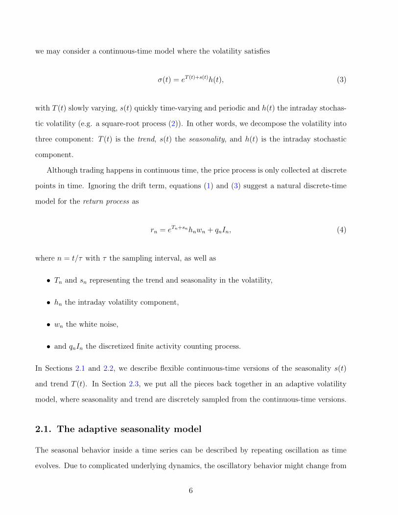
we may consider a continuous-time model where the volatility satisfies
σ(t) = eT (t)+s(t)h(t), (3)
with T (t) slowly varying, s(t) quickly time-varying and periodic and h(t) the intraday stochas-
tic volatility (e.g. a square-root process (2)). In other words, we decompose the volatility into
three component: T (t) is the trend, s(t) the seasonality, and h(t) is the intraday stochastic
component.
Although trading happens in continuous time, the price process is only collected at discrete
points in time. Ignoring the drift term, equations (1) and (3) suggest a natural discrete-time
model for the return process as
rn = eTn+snhnwn + qnIn, (4)
where n = t/τ with τ the sampling interval, as well as
• Tn and sn representing the trend and seasonality in the volatility,
• hn the intraday volatility component,
• wn the white noise,
• and qnIn the discretized finite activity counting process.
In Sections 2.1 and 2.2, we describe flexible continuous-time versions of the seasonality s(t)
and trend T (t). In Section 2.3, we put all the pieces back together in an adaptive volatility
model, where seasonality and trend are discretely sampled from the continuous-time versions.
2.1. The adaptive seasonality model
The seasonal behavior inside a time series can be described by repeating oscillation as time
evolves. Due to complicated underlying dynamics, the oscillatory behavior might change from
6
time to time. Intuitively, to capture this effect, we consider the adaptive seasonality model
s(t) =K∑k=1
ak(t) cos {2πkφ(t) + ξk} , (5)
where K ∈ N, ak(t) > 0, φ′(t) > 0, φ(0) = 0 and ξk ∈ R. The function ak(t) is called
the amplitude modulation (AM), φ(t) the phase function, ξk the phase shift, and φ′(t) the
instantaneous frequency (IF).
When the phase function is linear (ωt with ω > 0) and amplitude modulations are constant
(ak > 0 ∀k), then the model reduces to the Fourier Flexible Form (FFF) (see Gallant (1981)).
When the phase function is non-linear, the IF generalizes the concept of frequency, capturing
the number of oscillations one observes during an infinitesimal time period. As for the AM, it
represents the “instantaneous” magnitude of the oscillation.
While those time-varying quantities allow to capture momentary behavior, there is in gen-
eral no unique representation for an arbitrary s satisfying (5), even if K = 1. Indeed, there ex-
ists an infinity of smooth pairs of functions α(t) and β(t) so that cos(t) = {1 + α(t)} cos {t+ β(t)},
1 + α(t) > 0 and 1 + β′(t) > 0. This is known as the identifiability problem studied in Chen
et al. (2014). To resolve this issue, it is necessary to restrict the functional class and we borrow
the following definition from Chen et al. (2014):
Definition 1 (Intrinsic Mode Function Class Ac1,c2ε ). For fixed choices of 0 < ε � 1 and
ε � c1 < c2 < ∞, the space Ac1,c2ε of Intrinsic Mode Functions (IMFs) consists of functions
f : R→ R, f ∈ C1(R) ∩ L∞(R) having the form
f(t) = a(t) cos {2πφ(t)} , (6)
7
where a : R→ R and φ : R→ R satisfy the following conditions for all t ∈ R:
a ∈ C1(R) ∩ L∞(R), inft∈R
a(t) > c1, supt∈R
a(t) < c2, (7)
φ ∈ C2(R), inft∈R
φ′(t) > c1, supt∈R
φ′(t) < c2, (8)
|a′(t)| ≤ ε |φ′(t)|, |φ′′(t)| ≤ ε |φ′(t)|. (9)
This definition describes functions, referred to as IMF, mainly satisfying two requirements.
First, the AM and IF are both continuously differentiable and bounded from above and below.
Second, the rate of variation of both the AM and IF are small compared to the IF itself.
With the extra conditions on the IMF, the identifiability issue can be resolved in the following
way (Chen et al., 2014, Theorem 2.1). Suppose f(t) = a1(t) cos {2πφ1(t)} ∈ Ac1,c2ε can be
represented in a different form, for instance f(t) = a2(t) cos {2πφ2(t)}, which also satisfies the
conditions of Ac1,c2ε . Define α(t) = φ1(t) − φ2(t) and β(t) = a1(t) − a2(t), then α ∈ C2(R),
β ∈ C1(R) and |α′(t)| ≤ Cε, |α(t)| ≤ Cε and |β(t)| < Cε for all t ∈ R for a constant C
depending only on c1. In a nutshell, if a member of Ac1,c2ε can be represented in two different
forms, then the differences in phase function, AM and IF between the two forms are controllable
by the small model constant ε. In this sense, we are able to define AM and IF rigorously.
Because these conditions exclude jumps in AM and IF, in this paper, we make the working
assumption that the seasonality component of the market evolves slowly over time. As such,
we do not try to model abrupt changes. Note that the usual tests for structural breaks are
aimed at detecting if and where a break occurs, and they are not the modeling target of the
class Ac1,c2ε . To asses its validity when modeling financial data, we assume that the seasonality
belongs to the Ac1,c2ε class and resort to confidence interval estimation.
Note that the model from equation (5) comprises more than one oscillatory components.
To resolve the identifiability problem in this case, further conditions are necessary.
Definition 2 (Adaptive seasonality model Cc1,c2ε ). The space Cc1,c2ε of superpositions of IMFs
8
consists of functions f having the form
f(t) =K∑k=1
fk(t) and fk(t) = ak(t) cos {2πkφ(t) + ξk} (10)
for some finite K > 0 such that for each k = 1, . . . , K,
ξk ∈ R, ak(t) cos {2πkφ(t) + ξk} ∈ Ac1,c2ε and φ(0) = 0. (11)
Functions in the class Cc1,c2ε are composed of more than one IMF satisfying the condition
(11). In this case, an identifiability theorem similar to the one for Ac1,c2ε can be proved similarly
as that in (Chen et al., 2014, Theorem 2.2): if a member of Cc1,c2ε can be represented in two
different forms, then the two forms have the same number of IMFs, and the differences in their
phase function, AM and FM for each IMF are small. To summarize, with the Cc1,c2ε model and
its identifiability theorem, the IF and AM are well defined up to an uncertainty of order ε.
A popular member of Cc1,c2ε is the Fourier Flexible Form (FFF) (see Gallant (1981)), intro-
duced by Andersen and Bollerslev (1997, 1998) in the context of intraday seasonality. Using
Fourier series to decompose any periodic function into simple oscillating building blocks, a
simplified1 version of the FFF reads
s(t) =K∑k=1
[ak cos (2πkt) + bk sin (2πkt)] , (12)
where the sum of sines and cosines with integer frequencies captures the intraday patterns in the
volatility. Thus, we can view s(t) in (12) as a member of Cc1,c2ε with φ(t) = t, ξk = arctan(ak/bk)
and ak(t) =√a2k + b2
k for k = 1, . . . , K, that is with a fixed daily oscillation.
1Andersen and Bollerslev (1997, 1998) also consider the addition of dummy variables to capture weekdayeffects or particular events such as holidays in particular markets, but also unemployment reports, retail salesfigures, etc. While the periodic model captures most of the seasonal patterns, their dummy variables allow toquantify the relative importance of calendar effects and announcement events.
9
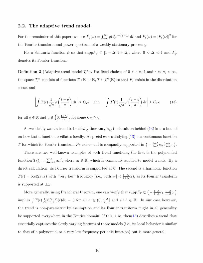
2.2. The adaptive trend model
For the remainder of this paper, we use Fy(ω) =∫∞−∞ y(t)e−i2πωtdt and Py(ω) = |Fy(ω)|2 for
the Fourier transform and power spectrum of a weakly stationary process y.
Fix a Schwartz function ψ so that suppFψ ⊂ [1 − ∆, 1 + ∆], where 0 < ∆ < 1 and Fψ
denotes its Fourier transform.
Definition 3 (Adaptive trend model T c1ε ). For fixed choices of 0 < ε � 1 and ε � c1 < ∞,
the space T c1ε consists of functions T : R→ R, T ∈ C1(R) so that FT exists in the distribution
sense, and
∣∣∣∣∫ T (t)1√aψ
(t− ba
)dt
∣∣∣∣ ≤ CT ε and
∣∣∣∣∫ T ′(t)1√aψ
(t− ba
)dt
∣∣∣∣ ≤ CT ε (13)
for all b ∈ R and a ∈(
0, 1+∆c1
], for some CT ≥ 0.
As we ideally want a trend to be slowly time-varying, the intuition behind (13) is as a bound
on how fast a function oscillates locally. A special case satisfying (13) is a continuous function
T for which its Fourier transform FT exists and is compactly supported in(− 1−∆
1+∆c1,
1−∆1+∆
c1
).
There are two well-known examples of such trend functions; the first is the polynomial
function T (t) =∑L
l=1 αltl, where αl ∈ R, which is commonly applied to model trends. By a
direct calculation, its Fourier transform is supported at 0. The second is a harmonic function
T (t) = cos(2πωt) with “very low” frequency (i.e., with |ω| < 1−∆1+∆
c1), as its Fourier transform
is supported at ±ω.
More generally, using Plancheral theorem, one can verify that suppFT ⊂(− 1−∆
1+∆c1,
1−∆1+∆
c1
)implies
∫T (t) 1√
aψ( t−b
a)(t)dt = 0 for all a ∈ (0, 1+∆
c1] and all b ∈ R. In our case however,
the trend is non-parametric by assumption and its Fourier transform might in all generality
be supported everywhere in the Fourier domain. If this is so, then(13) describes a trend that
essentially captures the slowly varying features of those models (i.e., its local behavior is similar
to that of a polynomial or a very low frequency periodic function) but is more general.
10
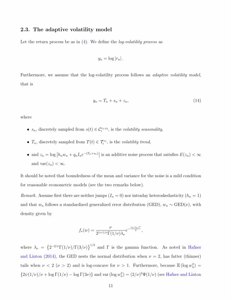
2.3. The adaptive volatility model
Let the return process be as in (4). We define the log-volatility process as
yn = log |rn| .
Furthermore, we assume that the log-volatility process follows an adaptive volatility model,
that is
yn = Tn + sn + zn, (14)
where
• sn, discretely sampled from s(t) ∈ Cc1,c2ε , is the volatility seasonality,
• Tn, discretely sampled from T (t) ∈ T c1ε , is the volatility trend,
• and zn = log∣∣hnwn + qnIne
−(Tn+sn)∣∣ is an additive noise process that satisfies E(zn) <∞
and var(zn) <∞.
It should be noted that boundedness of the mean and variance for the noise is a mild condition
for reasonable econometric models (see the two remarks below).
Remark. Assume first there are neither jumps (In = 0) nor intraday heteroskedasticity (hn = 1)
and that wn follows a standardized generalized error distribution (GED), wn ∼ GED(ν), with
density given by
fν(w) =ν
21+1/νΓ(1/ν)λνe−|w/λν |ν
2 ,
where λν ={
2−2/νΓ(1/ν)/Γ(3/ν)}1/2
and Γ is the gamma function. As noted in Hafner
and Linton (2014), the GED nests the normal distribution when ν = 2, has fatter (thinner)
tails when ν < 2 (ν > 2) and is log-concave for ν > 1. Furthermore, because E (logw2n) =
{2ψ(1/ν)/ν + log Γ(1/ν)− log Γ(3ν)} and var (logw2n) = (2/ν)2Ψ(1/ν) (see Hafner and Linton
11
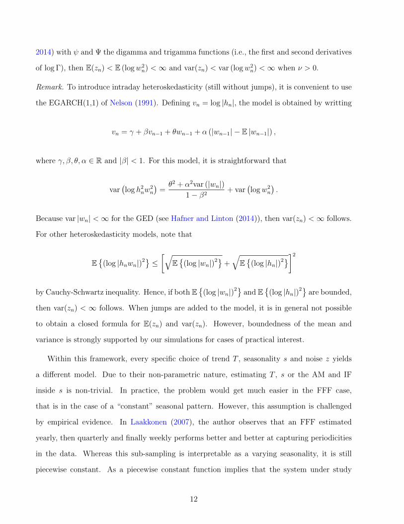
2014) with ψ and Ψ the digamma and trigamma functions (i.e., the first and second derivatives
of log Γ), then E(zn) < E (logw2n) <∞ and var(zn) < var (logw2
n) <∞ when ν > 0.
Remark. To introduce intraday heteroskedasticity (still without jumps), it is convenient to use
the EGARCH(1,1) of Nelson (1991). Defining vn = log |hn|, the model is obtained by writting
vn = γ + βvn−1 + θwn−1 + α (|wn−1| − E |wn−1|) ,
where γ, β, θ, α ∈ R and |β| < 1. For this model, it is straightforward that
var(log h2
nw2n
)=θ2 + α2var (|wn|)
1− β2+ var
(logw2
n
).
Because var |wn| <∞ for the GED (see Hafner and Linton (2014)), then var(zn) <∞ follows.
For other heteroskedasticity models, note that
E{
(log |hnwn|)2} ≤ [√E{
(log |wn|)2}+√
E{
(log |hn|)2}]2
by Cauchy-Schwartz inequality. Hence, if both E{
(log |wn|)2} and E{
(log |hn|)2} are bounded,
then var(zn) < ∞ follows. When jumps are added to the model, it is in general not possible
to obtain a closed formula for E(zn) and var(zn). However, boundedness of the mean and
variance is strongly supported by our simulations for cases of practical interest.
Within this framework, every specific choice of trend T , seasonality s and noise z yields
a different model. Due to their non-parametric nature, estimating T , s or the AM and IF
inside s is non-trivial. In practice, the problem would get much easier in the FFF case,
that is in the case of a “constant” seasonal pattern. However, this assumption is challenged
by empirical evidence. In Laakkonen (2007), the author observes that an FFF estimated
yearly, then quarterly and finally weekly performs better and better at capturing periodicities
in the data. Whereas this sub-sampling is interpretable as a varying seasonality, it is still
piecewise constant. As a piecewise constant function implies that the system under study
12
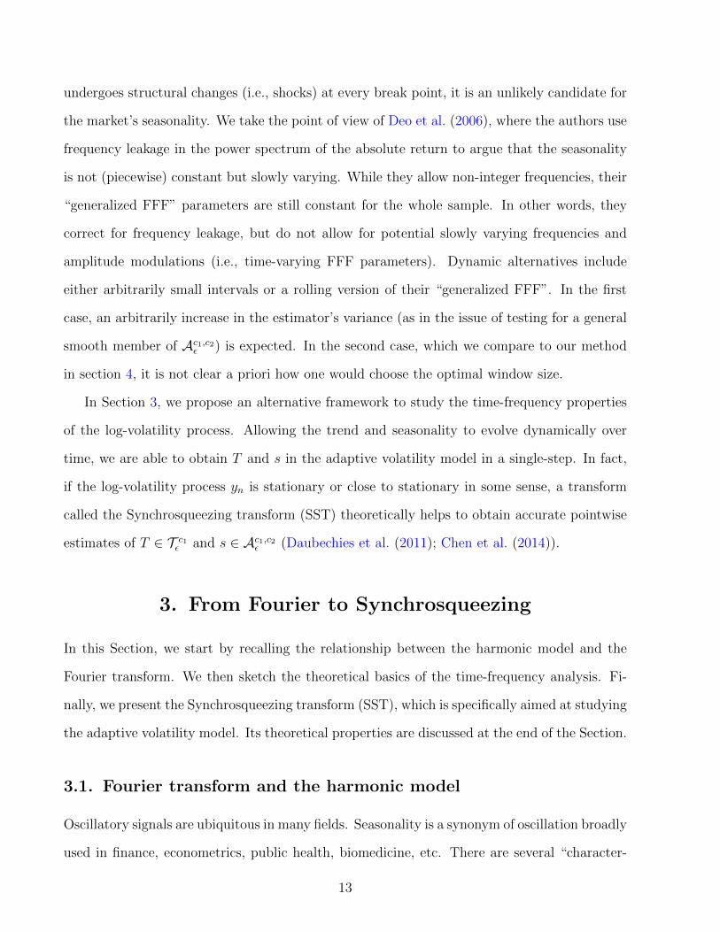
undergoes structural changes (i.e., shocks) at every break point, it is an unlikely candidate for
the market’s seasonality. We take the point of view of Deo et al. (2006), where the authors use
frequency leakage in the power spectrum of the absolute return to argue that the seasonality
is not (piecewise) constant but slowly varying. While they allow non-integer frequencies, their
“generalized FFF” parameters are still constant for the whole sample. In other words, they
correct for frequency leakage, but do not allow for potential slowly varying frequencies and
amplitude modulations (i.e., time-varying FFF parameters). Dynamic alternatives include
either arbitrarily small intervals or a rolling version of their “generalized FFF”. In the first
case, an arbitrarily increase in the estimator’s variance (as in the issue of testing for a general
smooth member of Ac1,c2ε ) is expected. In the second case, which we compare to our method
in section 4, it is not clear a priori how one would choose the optimal window size.
In Section 3, we propose an alternative framework to study the time-frequency properties
of the log-volatility process. Allowing the trend and seasonality to evolve dynamically over
time, we are able to obtain T and s in the adaptive volatility model in a single-step. In fact,
if the log-volatility process yn is stationary or close to stationary in some sense, a transform
called the Synchrosqueezing transform (SST) theoretically helps to obtain accurate pointwise
estimates of T ∈ T c1ε and s ∈ Ac1,c2ε (Daubechies et al. (2011); Chen et al. (2014)).
3. From Fourier to Synchrosqueezing
In this Section, we start by recalling the relationship between the harmonic model and the
Fourier transform. We then sketch the theoretical basics of the time-frequency analysis. Fi-
nally, we present the Synchrosqueezing transform (SST), which is specifically aimed at studying
the adaptive volatility model. Its theoretical properties are discussed at the end of the Section.
3.1. Fourier transform and the harmonic model
Oscillatory signals are ubiquitous in many fields. Seasonality is a synonym of oscillation broadly
used in finance, econometrics, public health, biomedicine, etc. There are several “character-
13
istics” one can use to describe an oscillatory signal (see Flandrin (1999)): for example, how
often an oscillation repeats itself “on average”, how large an oscillation is “on average”, etc.
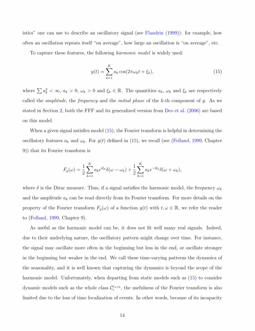
To capture these features, the following harmonic model is widely used:
y(t) =K∑k=1
ak cos(2πωkt+ ξk), (15)
where∑a2k < ∞, ak > 0, ωk > 0 and ξk ∈ R. The quantities ak, ωk and ξk are respectively
called the amplitude, the frequency and the initial phase of the k-th component of y. As we
stated in Section 2, both the FFF and its generalized version from Deo et al. (2006) are based
on this model.
When a given signal satisfies model (15), the Fourier transform is helpful in determining the
oscillatory features ak and ωk. For y(t) defined in (15), we recall (see (Folland, 1999, Chapter
9)) that its Fourier transform is
Fy(ω) =1
2
K∑k=1
akeiξkδ(ω − ωk) +
1
2
K∑k=1
ake−iξkδ(ω + ωk),
where δ is the Dirac measure. Thus, if a signal satisfies the harmonic model, the frequency ωk
and the amplitude ak can be read directly from its Fourier transform. For more details on the
property of the Fourier transform Fy(ω) of a function y(t) with t, ω ∈ R, we refer the reader
to (Folland, 1999, Chapter 9).
As useful as the harmonic model can be, it does not fit well many real signals. Indeed,
due to their underlying nature, the oscillatory pattern might change over time. For instance,
the signal may oscillate more often in the beginning but less in the end, or oscillate stronger
in the beginning but weaker in the end. We call these time-varying patterns the dynamics of
the seasonality, and it is well known that capturing the dynamics is beyond the scope of the
harmonic model. Unfortunately, when departing from static models such as (15) to consider
dynamic models such as the whole class Cc1,c2ε , the usefulness of the Fourier transform is also
limited due to the loss of time localization of events. In other words, because of its incapacity
14
to capture momentary behavior, we cannot use the Fourier transform to analyze the dynamics
of seasonality.
3.2. Time-frequency analysis
To overcome the limitation of the Fourier transform, time-frequency analysis was introduced
(see Daubechies (1992); Flandrin (1999) and the references inside for the historical discussion).
Heuristically, to capture the dynamics of the oscillatory signal, we take a small subset of
the given signal y(t) around a given time t0, and analyze its power spectrum. Ideally, this
provides information about the local behavior of y(t) around t0. We repeat the analysis at
all times, and the result is referred to as the time-frequency (TF) representation of the signal.
Mathematically, this idea is implemented by the short-time Fourier transform (STFT) and
continuous wavelet transform (CWT).
The STFT is defined by
Gy(t, ω) =
∫y(s) g(s− t) e−i2πωsds , (16)
where ω > 0 is frequency, and g is the window function associated with the STFT which
extracts the local signal for analysis. g has to be smooth enough and such that∫g(t)dt = 1.
The CWT is defined by
Wy(t, a) =
∫y(s) a−1/2 ψ
(s− ta
)ds , (17)
where a > 0. We call a the wavelet’s scale and ψ the mother wavelet which is smooth enough
and such that∫ψ(t)dt = 0.
In a nutshell, we select a subset of the whole signal by the window function or the mother
wavelet, and study how the signal oscillates locally. From the viewpoint of frame analysis, the
STFT and CWT are defined as the inner products between the signal to be analyzed and a
pre-assigned family of “templates”, or atoms – which are {g(· − t)e−i2πω·}ω∈R+,t∈R in STFT
15
and {a−1/2 ψ( ·−ta
)}a∈R+,t∈R in CWT. Furthermore, this inner product provides a way to resolve
events simultaneously in time (by translation) and frequency (by modulation and dilatation
respectively), but the properties of their respective templates yield different trade-offs between
temporal and frequency resolution due to the Heisenberg uncertainty principle. Take the high
frequency region for example. The STFT offers a better frequency resolution in frequency
events but an inferior resolution in time. In contrast, the CWT provides an inferior resolution
in frequency but a better resolution in time.
To further understand the time-frequency (TF) analysis, we consider the continuous wavelet
transform (CWT) of a purely harmonic signal y(t) = A cos(2πωt), and the same reasoning
follows for the short-time Fourier transform (STFT). From the Plancheral theorem, the CWT
of y becomes
Wy(t, a) = Aa1/2Fψ(ωa)ei2πωt. (18)
We observe that if Fψ(ω) is concentrated around ω = 1, then Wy(t, a) is concentrated around
a = 1/ω.
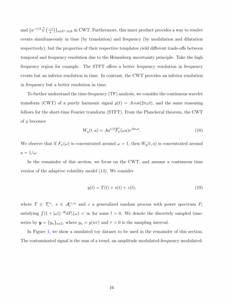
In the remainder of this section, we focus on the CWT, and assume a continuous time
version of the adaptive volatility model (14). We consider
y(t) = T (t) + s(t) + z(t), (19)
where T ∈ T c1ε , s ∈ Ac1,c2ε and z a generalized random process with power spectrum Pz
satisfying∫
(1 + |ω|)−2ldPz(ω) < ∞ for some l > 0. We denote the discretely sampled time-
series by y = {yn}n∈Z, where yn = y(nτ) and τ > 0 is the sampling interval.
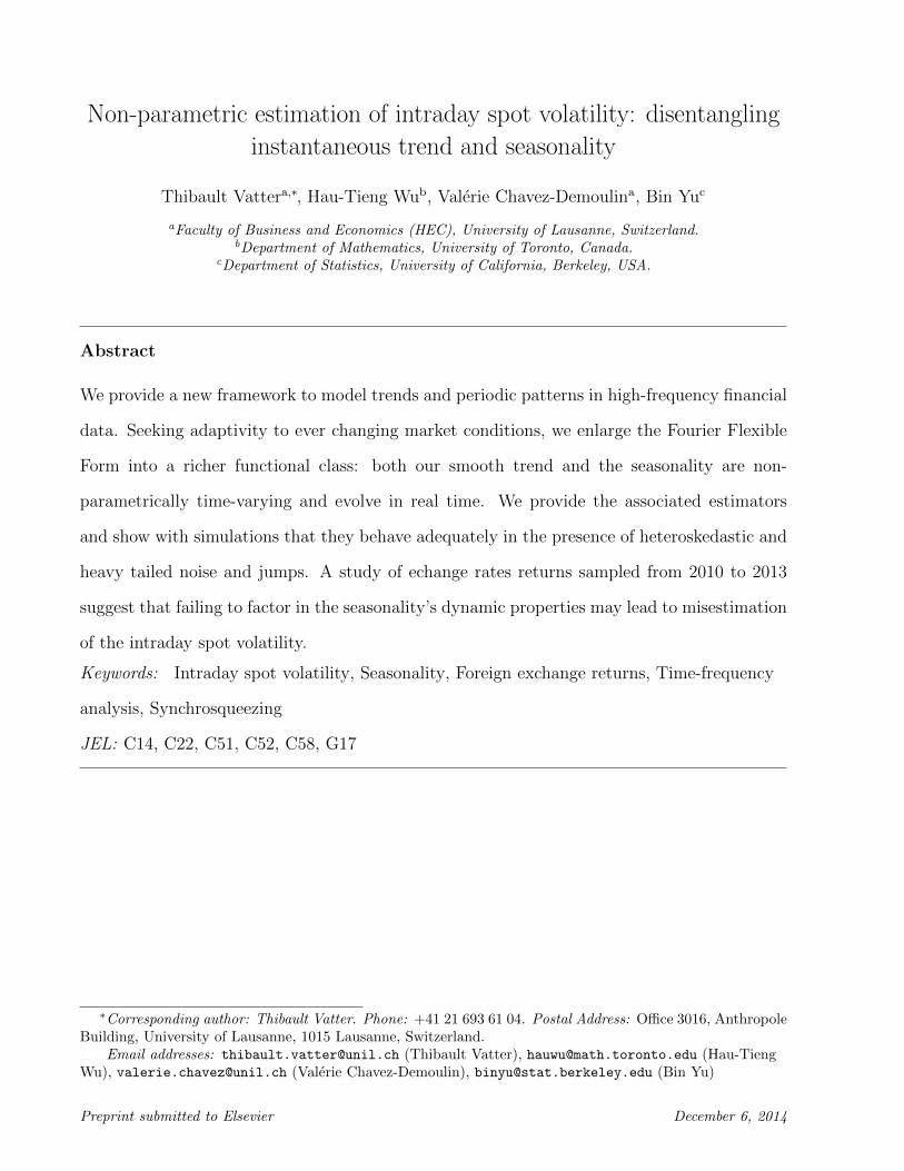
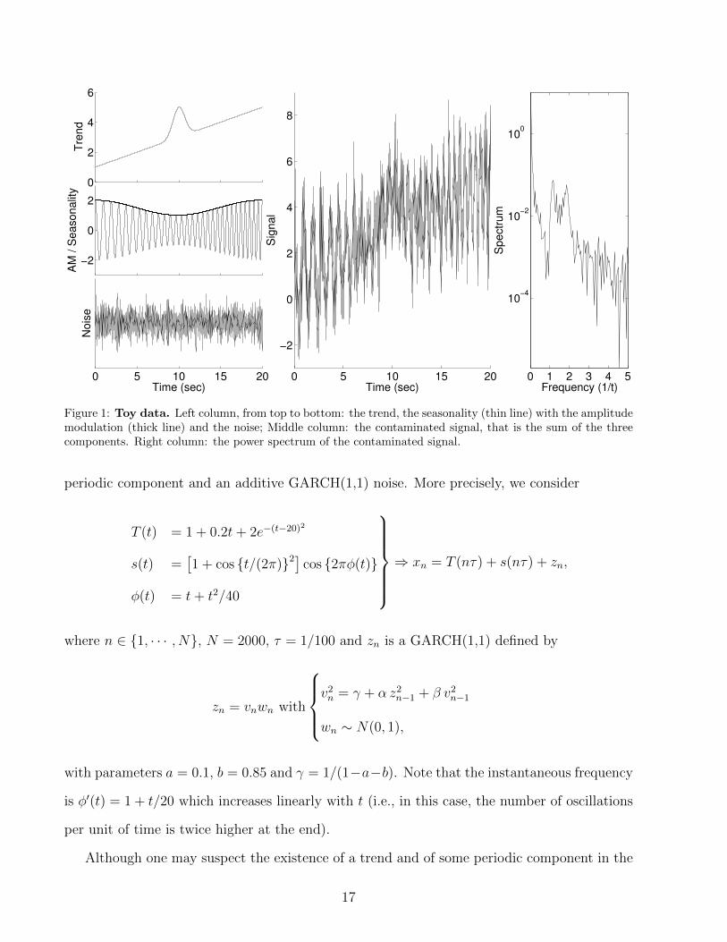
In Figure 1, we show a simulated toy dataset to be used in the remainder of this section.
The contaminated signal is the sum of a trend, an amplitude modulated-frequency modulated-
16
0 5 10 15 20
−2
0
2
4
6
8
Time (sec)
Sig
nal
0 1 2 3 4 5
10−4
10−2
100
Frequency (1/t)
Spectr
um
0
2
4
6
Tre
nd
−2
0
2
AM
/ S
easonalit
y
0 5 10 15 20Time (sec)
Nois
e
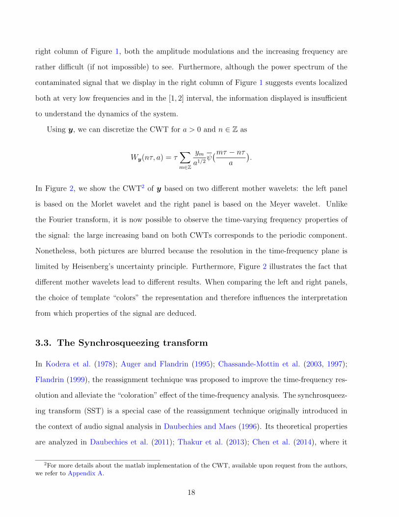
Figure 1: Toy data. Left column, from top to bottom: the trend, the seasonality (thin line) with the amplitudemodulation (thick line) and the noise; Middle column: the contaminated signal, that is the sum of the threecomponents. Right column: the power spectrum of the contaminated signal.
periodic component and an additive GARCH(1,1) noise. More precisely, we consider
T (t) = 1 + 0.2t+ 2e−(t−20)2
s(t) =[1 + cos {t/(2π)}2] cos {2πφ(t)}
φ(t) = t+ t2/40
⇒ xn = T (nτ) + s(nτ) + zn,
where n ∈ {1, · · · , N}, N = 2000, τ = 1/100 and zn is a GARCH(1,1) defined by
zn = vnwn with
v2n = γ + α z2
n−1 + β v2n−1
wn ∼ N(0, 1),
with parameters a = 0.1, b = 0.85 and γ = 1/(1−a−b). Note that the instantaneous frequency
is φ′(t) = 1 + t/20 which increases linearly with t (i.e., in this case, the number of oscillations
per unit of time is twice higher at the end).
Although one may suspect the existence of a trend and of some periodic component in the
17
right column of Figure 1, both the amplitude modulations and the increasing frequency are
rather difficult (if not impossible) to see. Furthermore, although the power spectrum of the
contaminated signal that we display in the right column of Figure 1 suggests events localized
both at very low frequencies and in the [1, 2] interval, the information displayed is insufficient
to understand the dynamics of the system.
Using y, we can discretize the CWT for a > 0 and n ∈ Z as
Wy(nτ, a) = τ∑m∈Z
yma1/2
ψ(mτ − nτ
a
).
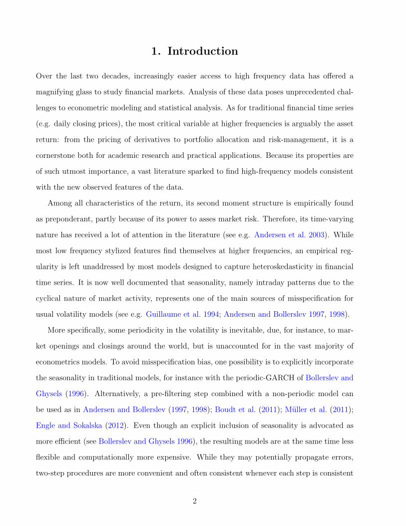
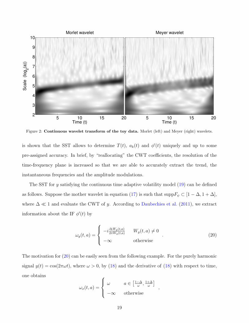
In Figure 2, we show the CWT2 of y based on two different mother wavelets: the left panel
is based on the Morlet wavelet and the right panel is based on the Meyer wavelet. Unlike
the Fourier transform, it is now possible to observe the time-varying frequency properties of
the signal: the large increasing band on both CWTs corresponds to the periodic component.
Nonetheless, both pictures are blurred because the resolution in the time-frequency plane is
limited by Heisenberg’s uncertainty principle. Furthermore, Figure 2 illustrates the fact that
different mother wavelets lead to different results. When comparing the left and right panels,
the choice of template “colors” the representation and therefore influences the interpretation
from which properties of the signal are deduced.
3.3. The Synchrosqueezing transform
In Kodera et al. (1978); Auger and Flandrin (1995); Chassande-Mottin et al. (2003, 1997);
Flandrin (1999), the reassignment technique was proposed to improve the time-frequency res-
olution and alleviate the “coloration” effect of the time-frequency analysis. The synchrosqueez-
ing transform (SST) is a special case of the reassignment technique originally introduced in
the context of audio signal analysis in Daubechies and Maes (1996). Its theoretical properties
are analyzed in Daubechies et al. (2011); Thakur et al. (2013); Chen et al. (2014), where it
2For more details about the matlab implementation of the CWT, available upon request from the authors,we refer to Appendix A.
18
Scale
(log
2(a
))
Morlet wavelet
Time (t)5 10 15 20
2
3
4
5
6
7
8
9
10Meyer wavelet
Time (t)5 10 15 20
Figure 2: Continuous wavelet transform of the toy data. Morlet (left) and Meyer (right) wavelets.
is shown that the SST allows to determine T (t), ak(t) and φ′(t) uniquely and up to some
pre-assigned accuracy. In brief, by “reallocating” the CWT coefficients, the resolution of the
time-frequency plane is increased so that we are able to accurately extract the trend, the
instantaneous frequencies and the amplitude modulations.
The SST for y satisfying the continuous time adaptive volatility model (19) can be defined
as follows. Suppose the mother wavelet in equation (17) is such that suppFψ ⊂ [1−∆, 1 + ∆],
where ∆� 1 and evaluate the CWT of y. According to Daubechies et al. (2011), we extract
information about the IF φ′(t) by
ωy(t, a) =
−i∂tWy(t,a)
2πWy(t,a)Wy(t, a) 6= 0
−∞ otherwise. (20)
The motivation for (20) can be easily seen from the following example. For the purely harmonic
signal y(t) = cos(2πωt), where ω > 0, by (18) and the derivative of (18) with respect to time,
one obtains
ωx(t, a) =
ω a ∈[
1−∆ω, 1+∆
ω
]−∞ otherwise
,
19
which is the desired information about its IF. Then the SST is defined by
Sy(t, ω) =
∫a : |Wy(t,a)|>Γ
Wy(t, a) a−3/2 δ {ωy(t, a)− ω } da, (21)
where Γ > 0 is the threshold chosen by the user, ω > 0 is the frequency and ωy(t, a) is defined
in (20). Keeping in mind that the frequency is reciprocally related to the scale, then (21) can
be understood as follows: based on the IF information ωy, at each time t, we collect the CWT
coefficients at scale a where a seasonal component with frequency close to ω is detected. This
additional step allows to mitigate the coloration due to the choice of template.
To discretize the SST, ωy is first obtained as
ωy(nτ, a) =
−i∂tWy(nτ, a)
2πWy(nτ, a)when |Wy(nτ, a)| 6= 0;
−∞ when |Wy(nτ, a)| = 0,
where ∂tWy(nτ, a) is defined as
∂tWy(nτ, a) = τ∑m∈Z
yma3/2
ψ′(mτ − nτ
a
).
Similarly, Sy(t, ω) is discretized as
Sy(nτ, ω) =
∫a: |Wy(nτ,a)|≥Γ
δ {|ωy(nτ, a)− ω|}Wy(nτ, a)a−3/2da.
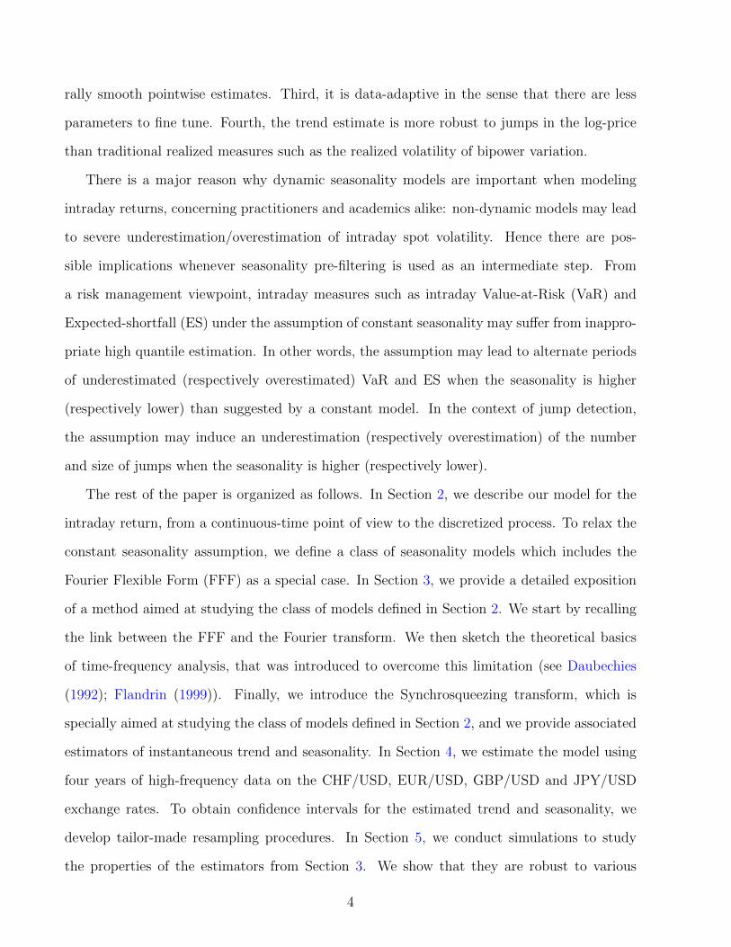
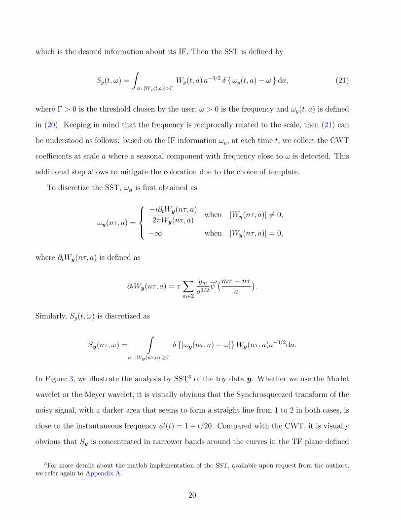
In Figure 3, we illustrate the analysis by SST3 of the toy data y. Whether we use the Morlet
wavelet or the Meyer wavelet, it is visually obvious that the Synchrosqueezed transform of the
noisy signal, with a darker area that seems to form a straight line from 1 to 2 in both cases, is
close to the instantaneous frequency φ′(t) = 1 + t/20. Compared with the CWT, it is visually
obvious that Sy is concentrated in narrower bands around the curves in the TF plane defined
3For more details about the matlab implementation of the SST, available upon request from the authors,we refer again to Appendix A.
20
Fre
quency (ω
)
Morlet wavelet
Time (t)5 10 15 20
5
4
3
2
1
Meyer wavelet
Time (t)5 10 15 20
Figure 3: Synchrosqueezed transform of the toy data. On the left: Morlet wavelet. On the right: Meyerwavelet.
by (t, kφ′(t)) (here with k = 1).
Using any curve extraction technique, it is possible to estimate the IF with high accuracy
and we denote this quantity as φ′. Furthermore, the restriction of Sy to the k-th narrow band
suffices to obtain an estimator of the k-th (complex) component of y as
fCk (nτ) =
1
Rψ
∫|kφ′(nτ)−ω|≤∆
Sy(nτ, ω)dω, (22)
where Rψ =∫ Fψ(ω)
ωdω. Then the corresponding estimator of the k-th (real) component fk and
amplitude modulations at time nτ are defined as
fk(nτ) = <{fCk (nτ)
}and ak(nτ) =
∣∣∣fCk (nτ)
∣∣∣ , (23)
where <(z) denotes the real part of z ∈ C. Finally, the restriction of Sy under a low-frequency
21
0 2 4 6 8 10 12 14 16 18 20−1
0
1
2
3
4
5
6
7
Time (sec)
Tru
e f
un
ctio
n v
s r
eco
nstr
ucte
d0
2
4
6
Tre
nd
1.1
1.3
1.5
1.7
1.9
IF
0 5 10 15 20
−2
0
2
Time (sec)
AM
/ S
ea
so
na
lity
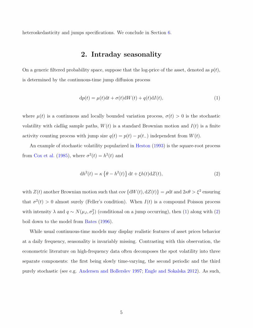
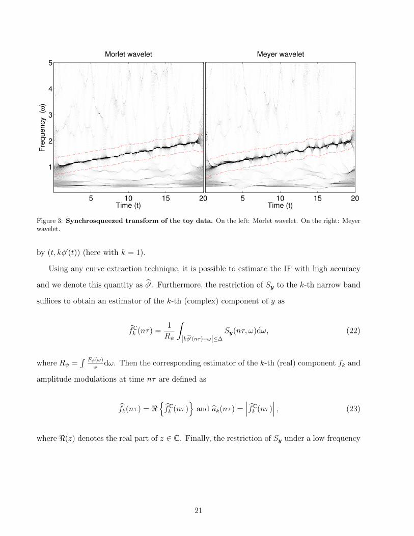
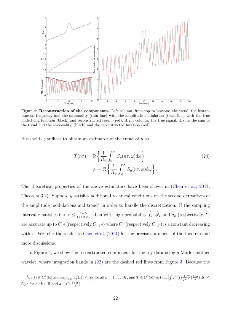
Figure 4: Reconstruction of the components. Left column, from top to bottom: the trend, the instan-taneous frequency and the seasonality (thin line) with the amplitude modulation (thick line) with the trueunderlying function (black) and reconstructed result (red); Right column: the true signal, that is the sum ofthe trend and the seasonality, (black) and the reconstructed function (red).
threshold ωl suffices to obtain an estimator of the trend of y as
T (nτ) = <{
1
Rψ
∫ ωl
0
Sy(nτ, ω)dω
}(24)
= yn −<{
1
Rψ
∫ ∞ωl
Sy(nτ, ω)dω
}.
The theoretical properties of the above estimators have been shown in (Chen et al., 2014,
Theorem 3.2). Suppose y satisfies additional technical conditions on the second derivatives of
the amplitude modulations and trend4 in order to handle the discretization. If the sampling
interval τ satisfies 0 < τ ≤ 1−∆(1+∆)c2
, then with high probability fk, φ′k and ak (respectively T )
are accurate up to Cτε (respectively Cτ,T ε) where Cτ (respectively Cτ,T ) is a constant decreasing
with τ . We refer the reader to Chen et al. (2014) for the precise statement of the theorem and
more discussions.
In Figure 4, we show the reconstructed component for the toy data using a Morlet mother
wavelet, where integration bands in (22) are the dashed red lines from Figure 3. Because the
4ak(t) ∈ C2(R) and supt∈R |a′′k(t)| ≤ εc2 for all k = 1, . . . ,K, and T ∈ C2(R) so that∣∣∣∫ T ′′(t) 1√
aψ(t−ba
)dt∣∣∣ ≤
CT ε for all b ∈ R and a ∈ (0, 1+∆c1
]
22
reconstruction is not dependent on the chosen mother wavelets5, it is not shown here for the
Meyer wavelet. Usually, while the instantaneous frequency is recovered precisely, the estimated
amplitude modulations are less ideal. Although this is important when the goal is forecasting,
it can be dampened by further smoothing the amplitude (here with a simple moving average
filter of length 1/τ).
In summary, for the harmonic model (15), the Fourier transform allows us to extract the
features of interest of the oscillation. When it comes to the adaptive volatility model (14), we
count on the synchrosqueezing transform to extract the oscillatory features of a given signal.
4. Application to foreign exchange data
As an empirical application, we study the EUR/USD, EUR/GBP, JPY/USD and USD/CHF
exchange rates from the beginning of 2010 to the end of 2013. We avoid the data preprocessing
by using pre-filtered 5-minute bid-ask pairs obtained from Dukascopy Bank SA6. The log-price
pn is computed as the average between the log bid and log ask prices and the return rn is
defined as the change between two consecutive log prices.
Because trading activity unquestionably drops during weekends and certain holidays (see
e.g. Dacorogna et al. 1993; Andersen and Bollerslev 1998), we exclude a number of days from
the sample, always from 21:05 GMT the night before until 21:00 GMT that evening. For
instance, weekends start on Friday at 21:05 GMT and last until Sunday at 21:00 GMT. Using
this definition of the trading day, we remove the fixed holidays of Christmas (December 24 -
December 26) and New Year’s (December 31 - January 2), as well as the moving holidays of
Martin Luther King’s Day, President’s Day, Good Friday, Memorial Day, July Fourth (also
when it is observed on July 3 or 5), Labor Day and Thanksgiving. After the cuts, we obtain
a sample of 998 days of data, containing 288 · 998 = 287424 intraday returns.
5This statement is correct up to the moments of the chosen mother wavelet ψ. The reconstruction errordepends on the first three moments of the chosen mother wavelet and its derivative but not on the profile of ψ(Daubechies et al. (2011); Chen et al. (2014))
6http://www.dukascopy.com/
23
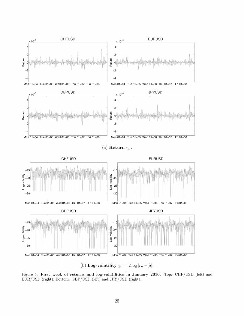
In panel 5a of Figure 5, we show the return rn for the four considered exchange rates
for the first week of trading, that is from January 3, 2010 (Sunday) at 21:05 pm GMT to
January 8, 2010 (Friday) at 21:00 pm GMT (1440 observations). While heteroskedasticity is
obviously present, it is arguably easier to discern its periodicity by looking at the log-volatility
yn = log |rn − µ| in panel 5b. Note that the smallest observations correspond to the case where
the price does not move during the 5 minutes interval (i.e., rn = 0 and yn = log |µ|).
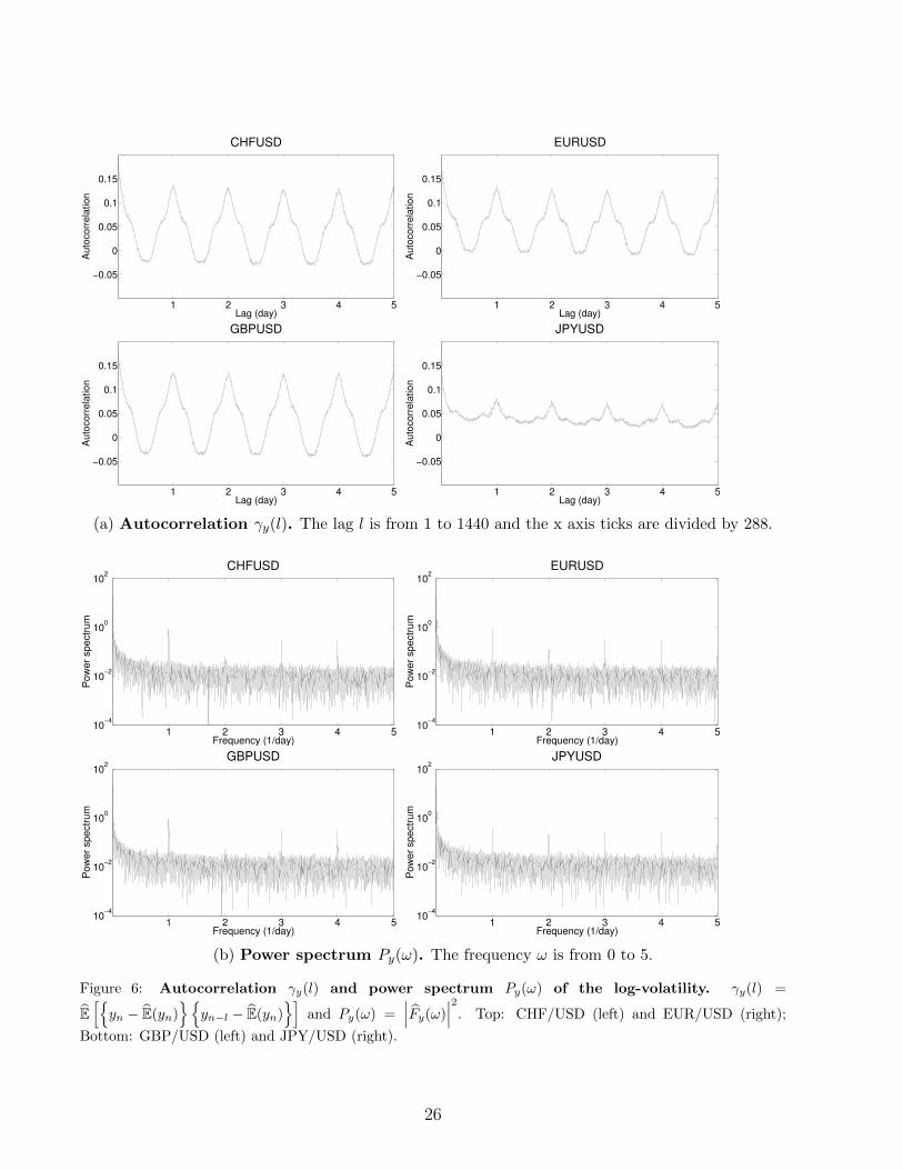
In Figure 6, the autocorrelation (Panel 6a) and the power spectrum (Panel 6b) of the log-
volatility indicate strong (daily) periodicities in the log-volatility. Although the shapes are
different for the various exchange rates, they all essentially display the same information: on
average, the seasonality is composed of periodic components of integer frequency. Note that
“on average” emphasizes the fact that both representations are only part of the picture. As
illustrated in Section 3, this representation misses the dynamics of the signal: for example, some
of the underlying periodic components may strengthen, weaken or even completely disappear
at some point. Another observation is that the JPY/USD curves are fairly different from the
others. First, according to the autocorrelation, the overall magnitude of oscillations (i.e., the
importance of the daily periodicity) is smaller. Second, according to the height of the power
spectrum’s second peak, the amplitude of the second component is much larger.
In Figure 7, we display |Sy(t, ω)|, the absolute value of the Synchrosqueezed transform,
in shades of gray for frequencies 0.5 ≤ ω ≤ 4.5. For all exchange rates, we observe much
darker curves (indicating higher values of |Sx(t, ω)|) at integer frequencies. As expected from
the power spectrums in Figure 6, the curves at 2 daily oscillations for all exchange rates
are very thin and sometimes fading, except for the JPY/USD. This apparent linearity of the
instantaneous frequency at integer values lends support for an amplitude-modulated version
of the FFF or, in other words, a member of Ac1,c2ε such that |φ(t)| = t. Although this kind
of constant frequency/amplitude modulated model can be estimated in different ways, we
carry the analysis within the SST framework. The red lines are the integration bands for the
reconstruction of the k-th periodic component using (22) and (23), that is at ω = k ±∆ with
k ∈ {1, 2, 3, 4} and ∆ = 0.02.
24
Mon 01−04 Tue 01−05 Wed 01−06 Thu 01−07 Fri 01−08
−4
−2
0
2
4
x 10−3 CHFUSD
Retu
rn
Mon 01−04 Tue 01−05 Wed 01−06 Thu 01−07 Fri 01−08
−4
−2
0
2
4
x 10−3 EURUSD
Retu
rn
Mon 01−04 Tue 01−05 Wed 01−06 Thu 01−07 Fri 01−08
−4
−2
0
2
4
x 10−3 GBPUSD
Retu
rn
Mon 01−04 Tue 01−05 Wed 01−06 Thu 01−07 Fri 01−08
−4
−2
0
2
4
x 10−3 JPYUSD
Retu
rn
(a) Return rn.
Mon 01−04 Tue 01−05 Wed 01−06 Thu 01−07 Fri 01−08
−30
−25
−20
−15
CHFUSD
Log−
vola
tilit
y
Mon 01−04 Tue 01−05 Wed 01−06 Thu 01−07 Fri 01−08
−30
−25
−20
−15
EURUSD
Log−
vola
tilit
y
Mon 01−04 Tue 01−05 Wed 01−06 Thu 01−07 Fri 01−08
−30
−25
−20
−15
GBPUSD
Log−
vola
tilit
y
Mon 01−04 Tue 01−05 Wed 01−06 Thu 01−07 Fri 01−08
−30
−25
−20
−15
JPYUSD
Log−
vola
tilit
y
(b) Log-volatility yn = 2 log |rn − µ|.
Figure 5: First week of returns and log-volatilities in January 2010. Top: CHF/USD (left) andEUR/USD (right); Bottom: GBP/USD (left) and JPY/USD (right).
25
1 2 3 4 5
−0.05
0
0.05
0.1
0.15
CHFUSD
Lag (day)
Au
toco
rre
latio
n
1 2 3 4 5
−0.05
0
0.05
0.1
0.15
EURUSD
Lag (day)
Au
toco
rre
latio
n
1 2 3 4 5
−0.05
0
0.05
0.1
0.15
GBPUSD
Lag (day)
Au
toco
rre
latio
n
1 2 3 4 5
−0.05
0
0.05
0.1
0.15
JPYUSD
Lag (day)
Au
toco
rre
latio
n
(a) Autocorrelation γy(l). The lag l is from 1 to 1440 and the x axis ticks are divided by 288.
1 2 3 4 510
−4
10−2
100
102
CHFUSD
Frequency (1/day)
Po
we
r sp
ectr
um
1 2 3 4 510
−4
10−2
100
102
EURUSD
Frequency (1/day)
Po
we
r sp
ectr
um
1 2 3 4 510
−4
10−2
100
102
GBPUSD
Frequency (1/day)
Po
we
r sp
ectr
um
1 2 3 4 510
−4
10−2
100
102
JPYUSD
Frequency (1/day)
Po
we
r sp
ectr
um
(b) Power spectrum Py(ω). The frequency ω is from 0 to 5.
Figure 6: Autocorrelation γy(l) and power spectrum Py(ω) of the log-volatility. γy(l) =
E[{yn − E(yn)
}{yn−l − E(yn)
}]and Py(ω) =
∣∣∣Fy(ω)∣∣∣2. Top: CHF/USD (left) and EUR/USD (right);
Bottom: GBP/USD (left) and JPY/USD (right).
26
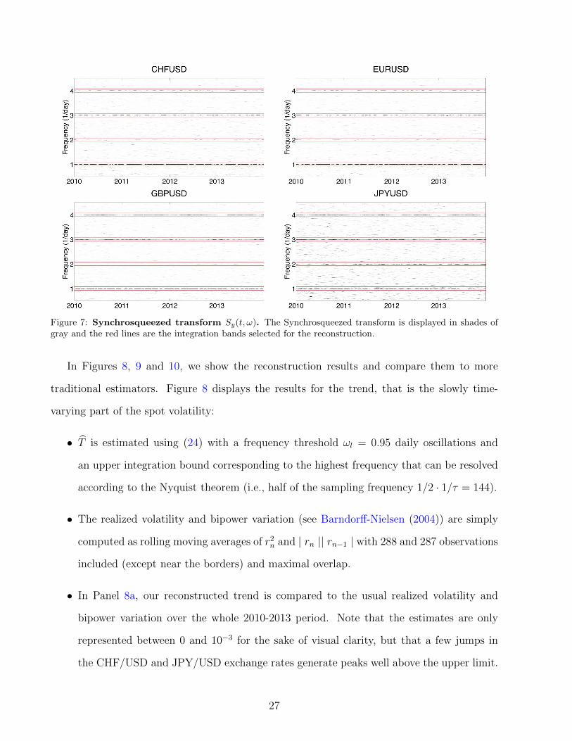
Figure 7: Synchrosqueezed transform Sy(t, ω). The Synchrosqueezed transform is displayed in shades ofgray and the red lines are the integration bands selected for the reconstruction.
In Figures 8, 9 and 10, we show the reconstruction results and compare them to more
traditional estimators. Figure 8 displays the results for the trend, that is the slowly time-
varying part of the spot volatility:
• T is estimated using (24) with a frequency threshold ωl = 0.95 daily oscillations and
an upper integration bound corresponding to the highest frequency that can be resolved
according to the Nyquist theorem (i.e., half of the sampling frequency 1/2 · 1/τ = 144).
• The realized volatility and bipower variation (see Barndorff-Nielsen (2004)) are simply
computed as rolling moving averages of r2n and | rn || rn−1 | with 288 and 287 observations
included (except near the borders) and maximal overlap.
• In Panel 8a, our reconstructed trend is compared to the usual realized volatility and
bipower variation over the whole 2010-2013 period. Note that the estimates are only
represented between 0 and 10−3 for the sake of visual clarity, but that a few jumps in
the CHF/USD and JPY/USD exchange rates generate peaks well above the upper limit.
27
• In Panel 8b, the three trend estimates are compared over a shorter time period in the
summer of 2011, that is in the middle of United States debt-ceiling crisis/European
sovereign debt crisis of 2011. Our reconstructed trend visibly constitutes a smoothed
version of the usual volatility measures, which usually fall inside the 95% confidence
interval except for upward spikes due to jumps. Notice the steep volatility increase
in all exchange rates as stock markets around the worlds started to fall following the
downgrading of America’s credit rating on 6 August 2011 by Standard & Poor’s. This
is especially true for the Swiss Franc, facing increasing pressure from currency markets
because considered a safe investment in times of economic uncertainty.
Figures 9 and 10 display the results for the amplitude modulations and seasonality:
• s is estimated using (22) and (23), as well as s(nτ) =∑K
k=1 fk(nτ).
• The Fourier Flexible Form/rolling Fourier Flexible Form (FFF/rFFF) are estimated us-
ing the ordinary least-square estimator on the whole sample/a four-weeks rolling window.
• In Figure 9, we show the amplitude modulations of the first periodic component. It is
noteworthy that when a unique FFF is estimated for the whole sample, the correspond-
ing amplitude is very close to the mean amplitude obtained with the SST. Furthermore,
we observe that the rFFF closely tracks the SST but is far wigglier. This was expected
because the SST estimator is essentially an instantaneous (and smooth by construction)
version of the FFF. Finally, notice that, as expected from Figure 6, the amplitude mod-
ulations of the first component in the JPY/USD are much smaller than the three other
exchange rates.
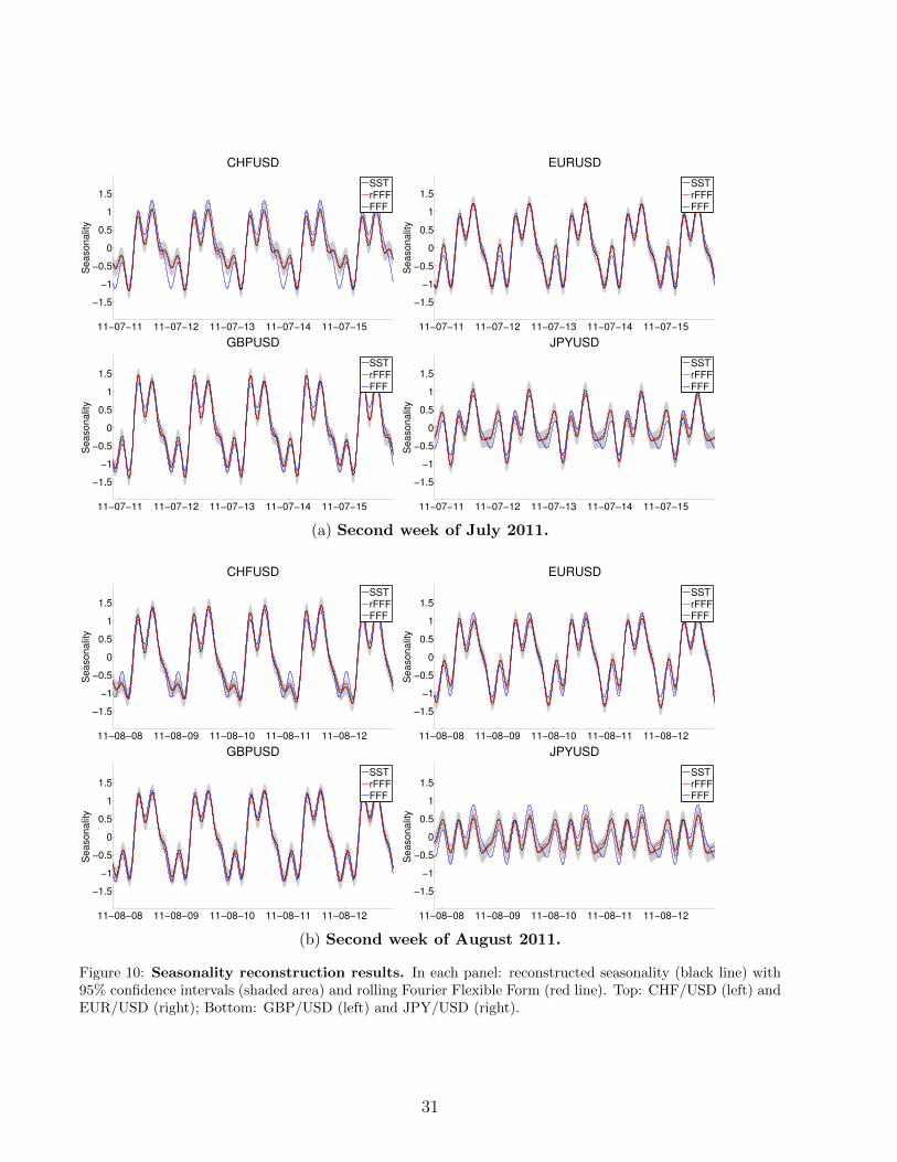
• In Panels 10a and 10b of Figure 10, we show the seasonality estimated as a sum of the
four periodic components: the FFF represents the average daily oscillation, the rFFF
is a wiggly estimate of the dynamics and the SST extracts a smooth instantaneous
seasonality. As in Figure 9, we observe that the overall magnitude of oscillation is much
smaller in the JPY/USD exchange rate.
28

2010 2011 2012 2013
0.2
0.4
0.6
0.8
x 10−3
Tre
nd
CHFUSD
exp(T)RVBV
2010 2011 2012 2013
0.2
0.4
0.6
0.8
x 10−3
Tre
nd
EURUSD
exp(T)RVBV
2010 2011 2012 2013
0.2
0.4
0.6
0.8
x 10−3
Tre
nd
GBPUSD
exp(T)RVBV
2010 2011 2012 2013
0.2
0.4
0.6
0.8
x 10−3
Tre
nd
JPYUSD
exp(T)RVBV
(a) Trend reconstruction for 2010-2013.
Jul 2011 Aug 2011 Sep 2011
0.2
0.4
0.6
0.8
x 10−3
Tre
nd
CHFUSD
exp(T)RVBV
Jul 2011 Aug 2011 Sep 2011
0.2
0.4
0.6
0.8
x 10−3
Tre
nd
EURUSD
exp(T)RVBV
Jul 2011 Aug 2011 Sep 2011
0.2
0.4
0.6
0.8
x 10−3
Tre
nd
GBPUSD
exp(T)RVBV
Jul 2011 Aug 2011 Sep 2011
0.2
0.4
0.6
0.8
x 10−3
Tre
nd
JPYUSD
exp(T)RVBV
(b) Zoom during the summer of 2011.
Figure 8: Trend reconstruction results. In each panel: reconstructed trend (black line), realized volatility(red line) and bipower variation (blue line). In Panel 8b: 95% confidence intervals for the reconstructed trend(shaded area). Top: CHF/USD (left) and EUR/USD (right); Bottom: GBP/USD (left) and JPY/USD (right).
29

2010 2011 2012 2013
0.2
0.6
1
1.4
Am
plit
ud
e 1
CHFUSD
SSTrFFFFFF
2010 2011 2012 2013
0.2
0.6
1
1.4
Am
plit
ud
e 1
EURUSD
SSTrFFFFFF
2010 2011 2012 2013
0.2
0.6
1
1.4
Am
plit
ud
e 1
GBPUSD
SSTrFFFFFF
2010 2011 2012 2013
0.2
0.6
1
1.4
Am
plit
ud
e 1
JPYUSD
SSTrFFFFFF
Figure 9: Amplitude modulations reconstruction results. In each panel: reconstructed amplitude mod-ulations of the first component (black line) with 95% confidence intervals (shaded area), Fourier Flexible Form(dashed line) and rolling Fourier Flexible Form (red line). Top: CHF/USD (left) and EUR/USD (right);Bottom: GBP/USD (left) and JPY/USD (right).
Remark. In Chen et al. (2014), the authors give theoretical bounds on the error committed
when reconstructing the trend and seasonality with the SST. However, those bounds have
two disadvantages: they are both very rough and impractical to implement. To obtain the
confidence intervals displayed in Figures 8, 9 and 10, we used the following procedure:
1. Use T (nτ) and fk(nτ) to recover the residuals
zn = yn − T (nτ)−K∑k=1
fk(nτ)
for n ∈ {1, · · · , N}.
2. Bootstrap B samples zbn for b ∈ {1, · · · , B} and n ∈ {1, · · · , N}.
3. Add back T (nτ) and fk(nτ) to zbn in order to obtain
ybn = zbn + T (nτ) +K∑k=1
fk(nτ)
30
11−07−11 11−07−12 11−07−13 11−07−14 11−07−15
−1.5
−1
−0.5
0
0.5
1
1.5
Se
aso
na
lity
CHFUSD
SSTrFFFFFF
11−07−11 11−07−12 11−07−13 11−07−14 11−07−15
−1.5
−1
−0.5
0
0.5
1
1.5
Se
aso
na
lity
EURUSD
SSTrFFFFFF
11−07−11 11−07−12 11−07−13 11−07−14 11−07−15
−1.5
−1
−0.5
0
0.5
1
1.5
Se
aso
na
lity
GBPUSD
SSTrFFFFFF
11−07−11 11−07−12 11−07−13 11−07−14 11−07−15
−1.5
−1
−0.5
0
0.5
1
1.5
Se
aso
na
lity
JPYUSD
SSTrFFFFFF
(a) Second week of July 2011.
11−08−08 11−08−09 11−08−10 11−08−11 11−08−12
−1.5
−1
−0.5
0
0.5
1
1.5
Se
aso
na
lity
CHFUSD
SSTrFFFFFF
11−08−08 11−08−09 11−08−10 11−08−11 11−08−12
−1.5
−1
−0.5
0
0.5
1
1.5
Se
aso
na
lity
EURUSD
SSTrFFFFFF
11−08−08 11−08−09 11−08−10 11−08−11 11−08−12
−1.5
−1
−0.5
0
0.5
1
1.5
Se
aso
na
lity
GBPUSD
SSTrFFFFFF
11−08−08 11−08−09 11−08−10 11−08−11 11−08−12
−1.5
−1
−0.5
0
0.5
1
1.5
Se
aso
na
lity
JPYUSD
SSTrFFFFFF
(b) Second week of August 2011.
Figure 10: Seasonality reconstruction results. In each panel: reconstructed seasonality (black line) with95% confidence intervals (shaded area) and rolling Fourier Flexible Form (red line). Top: CHF/USD (left) andEUR/USD (right); Bottom: GBP/USD (left) and JPY/USD (right).
31
for b ∈ {1, · · · , B} and n ∈ {1, · · · , N}.
4. Estimate T b(nτ) and f bk(nτ) for b ∈ {1, · · · , B} and n ∈ {1, · · · , N} to compute pointwise
confidence intervals.
As zn are found to be autocorrelated, a naive bootstrapping scheme is not appropriate. To
deal with this dependence issue, we use the automatic block-length selection procedure from
Politis and White (2004) along with circular block-bootstrap. In our case, the pointwise boot-
strapped distribution of the estimates is found to be approximately normal. However, a bias
correction proves to be necessary, which is achieved for instance for the trend by substracting
the bootstrapped bias∑B
b=1 Tb(nτ)/B − T (nτ) from the estimate T (nτ).
In summary, an impressing feature of our estimated trend is its robustness to jumps, which
affect both the realized volatility and, albeit to a lesser extent, the bipower variation. Regarding
the seasonality, Figures 9 and 10 strongly suggest that it evolves dynamically over time. Finally,
although similar estimates of trend and seasonality can be obtained with moving averages and
rolling regressions respectively, the SST provides smooth estimates and does not require an
arbitrary choice of the length of the window or the rolling overlap. One could argue that the
choice of mother wavelet is also arbitrary, but as illustrated in Section 2, the influence of this
choice on the SST estimators is negligible. In any case, the main message is that dynamic
methods are necessary to properly understand the seasonality, as static models can lead to
severe underestimation/overestimation of the intraday spot volatility.
5. Simulation study
In this section, we present simulations that use a realistic setting. To study the properties of the
estimators from Section 3, we directly sample 1000 times 150 days of data (i.e., 288·150 = 43200
observations) from the adaptive volatility model from equation (14), that is
yn = Tn + sn + zn,
32
where Tn and sn are deterministic functions and
zn = log∣∣hnwn + qnIne
−(Tn+sn)∣∣
with hn, wn and qnIn as described in Section 2. Using the EUR/USD sample (cf. Section 4, for
more details), we collect the first 150 days of extracted trend and seasonality, the latter either
with constant amplitude (estimated with the FFF) or with amplitude modulations (estimated
with the SST). Furthermore, we use the exponential of the estimated residuals (see Section
4) to obtain realistic parameters to simulate hnwn from either a GED(ν) (with hn = 1), an
EGARCH(1,1) or a GARCH(1,1). Finally, for the sake of simplicity, we assume that the two
components of the jump process are
• qn = eTn+snjn, where jn ∼ N(0, σj) with σj ∈ {4σw, 10σw} with σw the standard deviation
of the estimated i.i.d. GED(ν),
• and In ∼ B(1, λ) data) with λ ∈ {1/288, 1/1440}, that is one jump per day or week on
average.
Note that the assumption of proportionality to eTn+sn does not affect the following results.
In Figure 11, we show the results of a preliminary simulation study for both the trend and
seasonality with amplitude modulations when the noise is GED/GARCH with/without jumps,
where the case “with” is the most extreme (one 10 sigma jump per day). A striking feature
of the two panels is that there is basically no visible difference between the four kinds of noise
considered. Although not reported here, the pointwise biases and variances for the trend and
seasonality were also studied. While the biases were again indistinguishable (and basically
negligible for the trend) between the GED/GARCH with/without jumps, the variances were
higher for the GARCH with no visible effect from the jumps.
33

30 60 90 120
1
2
3
4
x 10−4
Days
Tre
nd
w ∼ GED, no jumps
estimated exp(trend)true exp(trend)
30 60 90 120
1
2
3
4
x 10−4
Days
Tre
nd
w ∼ GED, λj = 1/288, σj = 10σw
estimated exp(trend)true exp(trend)
30 60 90 120
1
2
3
4
x 10−4
Days
Tre
nd
w ∼ GARCH, no jumps
estimated exp(trend)true exp(trend)
30 60 90 120
1
2
3
4
x 10−4
Days
Tre
nd
w ∼ GARCH, λj = 1/288, σj = 10σw
estimated exp(trend)true exp(trend)
(a) Trend for the whole (simulated) data.
1 2 3 4
−1
0
1
Days
Se
aso
na
lity
w ∼ GED, no jumps
estimated seasonalitytrue seasonality
1 2 3 4
−1
0
1
Days
Se
aso
na
lity
w ∼ GED, λj = 1/288, σj = 10σw
estimated seasonalitytrue seasonality
1 2 3 4
−1
0
1
Days
Se
aso
na
lity
w ∼ GARCH, no jumps
estimated seasonalitytrue seasonality
1 2 3 4
−1
0
1
Days
Se
aso
na
lity
w ∼ GARCH, λj = 1/288, σj = 10σw
estimated seasonalitytrue seasonality
(b) Seasonality for the first week of the (simulated) data.
Figure 11: Trend and seasonality preliminary simulation results. In each panel: mean estimate (blackline), true quantity (red line) and estimated 95% confidence intervals (shaded area).
34
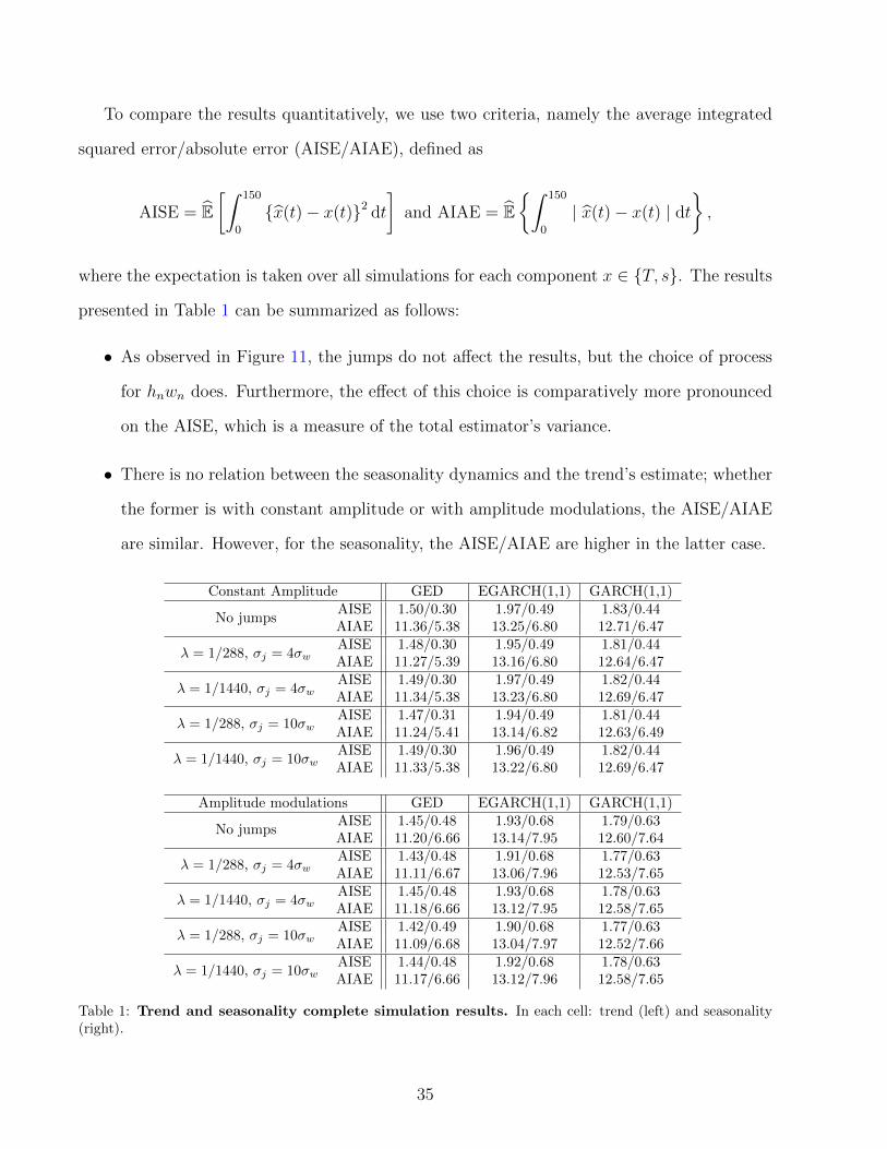
To compare the results quantitatively, we use two criteria, namely the average integrated
squared error/absolute error (AISE/AIAE), defined as
AISE = E[∫ 150
0
{x(t)− x(t)}2 dt
]and AIAE = E
{∫ 150
0
| x(t)− x(t) | dt},
where the expectation is taken over all simulations for each component x ∈ {T, s}. The results
presented in Table 1 can be summarized as follows:
• As observed in Figure 11, the jumps do not affect the results, but the choice of process
for hnwn does. Furthermore, the effect of this choice is comparatively more pronounced
on the AISE, which is a measure of the total estimator’s variance.
• There is no relation between the seasonality dynamics and the trend’s estimate; whether
the former is with constant amplitude or with amplitude modulations, the AISE/AIAE
are similar. However, for the seasonality, the AISE/AIAE are higher in the latter case.
Constant Amplitude GED EGARCH(1,1) GARCH(1,1)
No jumpsAISE 1.50/0.30 1.97/0.49 1.83/0.44AIAE 11.36/5.38 13.25/6.80 12.71/6.47
λ = 1/288, σj = 4σwAISE 1.48/0.30 1.95/0.49 1.81/0.44AIAE 11.27/5.39 13.16/6.80 12.64/6.47
λ = 1/1440, σj = 4σwAISE 1.49/0.30 1.97/0.49 1.82/0.44AIAE 11.34/5.38 13.23/6.80 12.69/6.47
λ = 1/288, σj = 10σwAISE 1.47/0.31 1.94/0.49 1.81/0.44AIAE 11.24/5.41 13.14/6.82 12.63/6.49
λ = 1/1440, σj = 10σwAISE 1.49/0.30 1.96/0.49 1.82/0.44AIAE 11.33/5.38 13.22/6.80 12.69/6.47
Amplitude modulations GED EGARCH(1,1) GARCH(1,1)
No jumpsAISE 1.45/0.48 1.93/0.68 1.79/0.63AIAE 11.20/6.66 13.14/7.95 12.60/7.64
λ = 1/288, σj = 4σwAISE 1.43/0.48 1.91/0.68 1.77/0.63AIAE 11.11/6.67 13.06/7.96 12.53/7.65
λ = 1/1440, σj = 4σwAISE 1.45/0.48 1.93/0.68 1.78/0.63AIAE 11.18/6.66 13.12/7.95 12.58/7.65
λ = 1/288, σj = 10σwAISE 1.42/0.49 1.90/0.68 1.77/0.63AIAE 11.09/6.68 13.04/7.97 12.52/7.66
λ = 1/1440, σj = 10σwAISE 1.44/0.48 1.92/0.68 1.78/0.63AIAE 11.17/6.66 13.12/7.96 12.58/7.65
Table 1: Trend and seasonality complete simulation results. In each cell: trend (left) and seasonality(right).
35
6. Discussion
Our disentangling of instantaneous trend and seasonality of the intraday spot volatility is an
extension of classical econometric models that provides adaptivity to ever changing markets.
The proposed method suggests a realistic framework for the high frequency time series behav-
ior. First, it lets the realized volatility be modeled as an instantaneous trend which evolves in
real time within the day. Second, it allows the seasonality to be non-constant over the sample.
In a simulation study using a realistic setting, numerical results confirm that the proposed
estimators for the trend and seasonality components have an appropriate behavior. We show
that this result holds even in presence of heteroskedastic and heavy tailed noise and is also
robust to jumps.
Using the CHF/USD, EUR/USD, GBP/USD and USD/JPY exchange rates sampled every
5 minutes between 2010 and 2013, we confirm empirically that the oscillation frequency is
constant, as suggested originally in the Fourier Flexible Form from Andersen and Bollerslev
(1997, 1998). In the four exchange rates, we show that the amplitude modulations of the
periodic components and hence the overall magnitude of oscillation evolve dynamically over
time. As such, neglecting those modulations in the periodic part of the volatility would imply
either an overestimation (when the periodic components are lower than their mean value)
or an underestimation (when the periodic components are higher than their mean value).
Furthermore, we show that the SST estimator gives results comparable to a smooth version of
a rolling Fourier Flexible Form. However, the adaptivity of SST should still be emphasized,
as it does not require ad-hoc choices neither of the rolling overlapping ratio nor of the length
of each window as for a parametric regression.
While we illustrate our model by simultaneously disentangling the low and high frequency
components of the intraday spot volatility in the FX market, it is possible to embed the new
methodology into a forecasting exercise. Although this is beyond the scope of the present paper,
which is rather aimed at presenting the modeling framework, the exercise may be useful in
the context of an investor’s optimal portfolio choice or for risk-management purposes. Further
36
research directions include the extension of the framework to both the non-homogeneously
sampled (“tick-by-tick”) as well as multivariate data. We will return to these questions and
related issues in future works.
Acknowledgements
Most of this research was conducted while the corresponding author was visiting the Berkeley
Statistics Department. He is grateful for its support and helpful discussions with the members
both in Bin Yu’s research group and the Coleman Fung Risk Management Research Center.
This research is also supported in part by the Center for Science of Information (CSoI), a US
NSF Science and Technology Center, under grant agreement CCF-0939370, and by NSF grants
DMS-1160319 and CDS&E-MSS 1228246.
References
Andersen, T. G. and Bollerslev, T. (1997), “Intraday periodicity and volatility persistence in
financial markets,” Journal of Empirical Finance, 4, 115–158.
— (1998), “Deutsche Mark - Dollar Volatility : Intraday Activity Patterns , Macroeconomic
Announcements,” The Journal of Finance, 53, 219–265.
Andersen, T. G., Bollerslev, T., Diebold, F. X., and Labys, P. (2003), “Modeling and Fore-
casting Realized Volatility,” Econometrica, 71, 579–625.
Auger, F. and Flandrin, P. (1995), “Improving the readability of time-frequency and time-scale
representations by the reassignment method,” IEEE Trans. Signal Process., 43, 1068–1089.
Barndorff-Nielsen, O. E. (2004), “Power and Bipower Variation with Stochastic Volatility and
Jumps,” Journal of Financial Econometrics, 2, 1–37.
37
Bates, D. S. (1996), “Jumps and stochastic volatility: exchange rate processes implicit in
deutsche mark options,” Review of Financial Studies, 9, 69–107.
Bollerslev, T. and Ghysels, E. (1996), “Periodic autoregressive conditional heteroscedasticity,”
Journal of Business & Economic Statistics, 14, 139–151.
Boudt, K., Croux, C., and Laurent, S. (2011), “Robust estimation of intraweek periodicity in
volatility and jump detection,” Journal of Empirical Finance, 18, 353–367.
Chassande-Mottin, E., Auger, F., and Flandrin, P. (2003), “Time-frequency/time-scale reas-
signment,” in Wavelets and signal processing, Boston, MA: Birkhauser Boston, Appl. Numer.
Harmon. Anal., pp. 233–267.
Chassande-Mottin, E., Daubechies, I., Auger, F., and Flandrin, P. (1997), “Differential reas-
signment,” Signal Processing Letters, IEEE, 4, 293–294.
Chen, Y.-C., Cheng, M.-Y., and Wu, H.-T. (2014), “Non-parametric and adaptive modelling
of dynamic periodicity and trend with heteroscedastic and dependent errors,” Journal of the
Royal Statistical Society: Series B (Statistical Methodology), 76, 651–682.
Cox, J. C., Ingersoll Jonathan E., J., and Ross, S. A. (1985), “A Theory of the Term Structure
of Interest Rates,” Econometrica, 53, 385–407.
Dacorogna, M. M., Muller, U. A., Nagler, R. J., Olsen, R. B., and Pictet, O. V. (1993),
“A geographical model for the daily and weekly seasonal volatility in the foreign exchange
market,” Journal of International Money and Finance, 12, 413–438.
Daubechies, I. (1992), Ten Lectures on Wavelets, Philadelphia: Society for Industrial and
Applied Mathematics.
Daubechies, I., Lu, J., and Wu, H.-T. (2011), “Synchrosqueezed wavelet transforms: An em-
pirical mode decomposition-like tool,” Applied and Computational Harmonic Analysis, 30,
243–261.
38

Daubechies, I. and Maes, S. (1996), “A nonlinear squeezing of the continuous wavelet transform
based on auditory nerve models,” in Wavelets in Medicine and Biology, CRC-Press, pp. 527–
546.
Deo, R., Hurvich, C., and Lu, Y. (2006), “Forecasting realized volatility using a long-memory
stochastic volatility model: estimation, prediction and seasonal adjustment,” Journal of
Econometrics, 131, 29–58.
Engle, R. F. and Sokalska, M. E. (2012), “Forecasting intraday volatility in the US equity
market. Multiplicative component GARCH,” Journal of Financial Econometrics, 10, 54–83.
Flandrin, P. (1999), Time-frequency/time-scale Analysis, Wavelet Analysis and Its Applica-
tions, Academic Press Inc.
Folland, G. B. (1999), Real Analysis: Modern Techniques and Their Applications, Wiley-
Interscience.
Gallant, R. (1981), “On the bias in flexible functional forms and an essentially unbiased form:
The fourier flexible form,” Journal of Econometrics, 15, 211–245.
Giot, P. (2005), “Market risk models for intraday data,” The European Journal of Finance,
11, 309–324.
Guillaume, D. M., Pictet, O. V., and Dacorogna, M. M. (1994), “On the intra-daily perfor-
mance of GARCH processes,” Working papers, Olsen and Associates.
Hafner, C. M. and Linton, O. (2014), “An almost closed form estimator for the EGARCH
model,” SSRN Electronic Journal.
Heston, S. L. (1993), “A closed-form solution for options with stochastic volatility with appli-
cations to bond and currency options,” Review of Financial Studies, 6, 327–343.
Kodera, K., Gendrin, R., and Villedary, C. (1978), “Analysis of time-varying signals with small
BT values,” Acoustics, Speech and Signal Processing, IEEE Transactions on, 26, 64–76.
39
Laakkonen, H. (2007), “Exchange rate volatility, macro announcements and the choice of in-
traday seasonality filtering method,” Research Discussion Papers 23/2007, Bank of Finland.
Martens, M., Chang, Y.-C., and Taylor, S. J. (2002), “A comparison of seasonal adjustment
methods when forecasting intraday volatility,” The Journal of Financial Research, 25, 283–
299.
Muller, H.-G., Sen, R., and Stadtmuller, U. (2011), “Functional data analysis for volatility,”
Journal of Econometrics, 165, 233–245.
Nelson, D. B. (1991), “Conditional heteroskedasticity in asset returns a new approach,” Econo-
metrica, 29, 347–370.
Newey, W. K. and McFadden, D. (1994), “Large sample estimation and hypothesis testing,” in
Handbook of Econometrics, eds. Engle, R. F. and McFadden, D. L., Elsevier North Holland,
vol. 4, pp. 2111–2245.
Politis, D. N. and White, H. (2004), “Automatic Block-Length Selection for the Dependent
Bootstrap,” Econometric Reviews, 23, 53–70.
Thakur, G., Brevdo, E., Fuckar, N. S., and Wu, H.-T. (2013), “The Synchrosqueezing algorithm
for time-varying spectral analysis: robustness properties and new paleoclimate applications,”
Signal Processing, 93, 1079–1094.
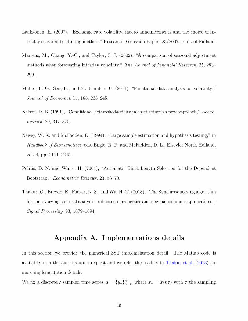
Appendix A. Implementations details
In this section we provide the numerical SST implementation detail. The Matlab code is
available from the authors upon request and we refer the readers to Thakur et al. (2013) for
more implementation details.
We fix a discretely sampled time series y = {yn}Nn=1, where xn = x(nτ) with τ the sampling
40
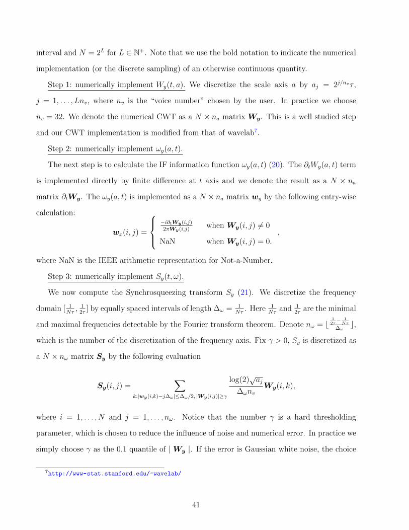
interval and N = 2L for L ∈ N+. Note that we use the bold notation to indicate the numerical
implementation (or the discrete sampling) of an otherwise continuous quantity.
Step 1: numerically implement Wy(t, a). We discretize the scale axis a by aj = 2j/nvτ ,
j = 1, . . . , Lnv, where nv is the “voice number” chosen by the user. In practice we choose
nv = 32. We denote the numerical CWT as a N × na matrix Wy. This is a well studied step
and our CWT implementation is modified from that of wavelab7.
Step 2: numerically implement ωy(a, t).
The next step is to calculate the IF information function ωy(a, t) (20). The ∂tWy(a, t) term
is implemented directly by finite difference at t axis and we denote the result as a N × na
matrix ∂tWy. The ωy(a, t) is implemented as a N × na matrix wy by the following entry-wise
calculation:
wx(i, j) =
−i∂tWy(i,j)
2πWy(i,j)when Wy(i, j) 6= 0
NaN when Wy(i, j) = 0.,
where NaN is the IEEE arithmetic representation for Not-a-Number.
Step 3: numerically implement Sy(t, ω).
We now compute the Synchrosqueezing transform Sy (21). We discretize the frequency
domain [ 1Nτ, 1
2τ] by equally spaced intervals of length ∆ω = 1
Nτ. Here 1
Nτand 1
2τare the minimal
and maximal frequencies detectable by the Fourier transform theorem. Denote nω = b12τ− 1Nτ
∆ωc,
which is the number of the discretization of the frequency axis. Fix γ > 0, Sy is discretized as
a N × nω matrix Sy by the following evaluation
Sy(i, j) =∑
k:|wy(i,k)−j∆ω |≤∆ω/2, |Wy(i,j)|≥γ
log(2)√aj
∆ωnvWy(i, k),
where i = 1, . . . , N and j = 1, . . . , nω. Notice that the number γ is a hard thresholding
parameter, which is chosen to reduce the influence of noise and numerical error. In practice we
simply choose γ as the 0.1 quantile of |Wy |. If the error is Gaussian white noise, the choice
7http://www-stat.stanford.edu/~wavelab/
41
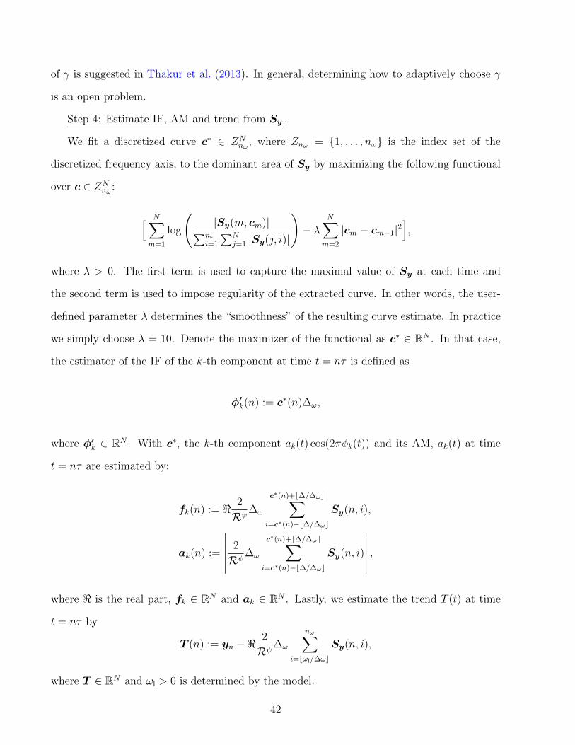
of γ is suggested in Thakur et al. (2013). In general, determining how to adaptively choose γ
is an open problem.
Step 4: Estimate IF, AM and trend from Sy.
We fit a discretized curve c∗ ∈ ZNnω , where Znω = {1, . . . , nω} is the index set of the
discretized frequency axis, to the dominant area of Sy by maximizing the following functional
over c ∈ ZNnω :
[ N∑m=1
log
(|Sy(m, cm)|∑nω
i=1
∑Nj=1 |Sy(j, i)|
)− λ
N∑m=2
|cm − cm−1|2],
where λ > 0. The first term is used to capture the maximal value of Sy at each time and
the second term is used to impose regularity of the extracted curve. In other words, the user-
defined parameter λ determines the “smoothness” of the resulting curve estimate. In practice
we simply choose λ = 10. Denote the maximizer of the functional as c∗ ∈ RN . In that case,
the estimator of the IF of the k-th component at time t = nτ is defined as
φ′k(n) := c∗(n)∆ω,
where φ′k ∈ RN . With c∗, the k-th component ak(t) cos(2πφk(t)) and its AM, ak(t) at time
t = nτ are estimated by:
fk(n) := < 2
Rψ∆ω
c∗(n)+b∆/∆ωc∑i=c∗(n)−b∆/∆ωc
Sy(n, i),
ak(n) :=
∣∣∣∣∣∣ 2
Rψ∆ω
c∗(n)+b∆/∆ωc∑i=c∗(n)−b∆/∆ωc
Sy(n, i)
∣∣∣∣∣∣ ,where < is the real part, fk ∈ RN and ak ∈ RN . Lastly, we estimate the trend T (t) at time
t = nτ by
T (n) := yn −<2
Rψ∆ω
nω∑i=bωl/∆ωc
Sy(n, i),
where T ∈ RN and ωl > 0 is determined by the model.
42


