Embed Size (px)
Citation preview

Georgetown University Law CenterScholarship @ GEORGETOWN LAW
2012
vGUPPI: Scoring Unilateral Pricing Incentives inVertical MergersSerge MoresiCharles River Associates (CRA), [email protected]
Steven C. SalopGeorgetown University Law Center, [email protected]
Georgetown Business, Economics and Regulatory Law Research Paper No. 12-022
This paper can be downloaded free of charge from:http://scholarship.law.georgetown.edu/fwps_papers/163http://ssrn.com/abstract=2085999
This open-access article is brought to you by the Georgetown Law Library. Posted with permission of the author.Follow this and additional works at: http://scholarship.law.georgetown.edu/fwps_papers
Part of the Antitrust and Trade Regulation Commons, Corporation and Enterprise Law Commons, and the Econometrics Commons

1
vGUPPI: Scoring Unilateral Pricing Incentives in Vertical Mergers
Serge Moresi1
Steven C. Salop2
February 5, 2013
I. Introduction
Vertical mergers can raise a variety of competitive concerns, including
foreclosure, coordination, and misuse of sensitive competitive information. One key
concern is input foreclosure. Input foreclosure involves raising the costs of competitors
in the downstream market.3 For example, a vertical merger between an input supplier
and a downstream output manufacturer can create unilateral incentives for the supplier to
raise the price of its inputs to one or several “targeted” competitors of the manufacturer.4
The higher input prices could raise the costs of the downstream rivals, which could in
1 Vice President and Director of Competition Modeling, Charles River Associates (CRA). 2 Professor of Economics and Law, Georgetown University Law Center and Senior Consultant, CRA. 3 Input foreclosure is different from customer foreclosure, which involves reducing sales opportunities, and hence the revenues, of the upstream input competitors by denying them the ability to sell inputs to the downstream merging firm. For a discussion of both foreclosure concepts in the context of vertical mergers, see Michael H. Riordan & Steven C. Salop, Evaluating Vertical Mergers: A Post-Chicago Approach, 63 ANTITRUST L.J. 513 (1995). For other analyses of vertical mergers, see Jeffrey Church, Vertical Mergers, in 2 ISSUES IN COMPETITION LAW AND POL’Y 1455 (2008); Michael H. Riordan, Competitive Effects of Vertical Integration, in HANDBOOK ANTITRUST ECON. 145 (Paolo Buccirossi, ed., 2008); and the sources cited therein. See also EUROPEAN COMMISSION, GUIDELINES ON THE ASSESSMENT OF NONHORIZONTAL MERGERS UNDER THE COUNCIL REGULATION ON THE CONTROL OF CONCENTRATIONS BETWEEN UNDERTAKINGS, 2008 O.J. (C 265) 6, available at http://eur-lex.europa.eu/LexUriServ/LexUriServ.do? uri=OJ:C:2008:265:0006:0025:EN:PDF (adopted on Nov. 28, 2007 and published on Oct. 18, 2008) (hereinafter, E.C. Non-Horizontal Merger Guidelines). For a general framework, see Thomas G. Krattenmaker & Steven C. Salop, Anticompetitive Exclusion: Raising Rivals' Costs to Achieve Power Over Price, 96 YALE L.J. 209 (1986). 4 A similar concern applies to complementary product mergers. The merger may lead the merged firms to refuse to deal with or raise the price of the complements to competitors that are not integrated.

2
turn increase the sales and profits of the downstream merger partner. These effects could
lead the downstream firms to raise prices and harm consumers.
Vertical mergers also can increase competition by the creation of efficiencies.5
Vertically related firms must cooperate to some degree to bring products to market. This
creates greater opportunities for efficiency gains than for horizontal mergers. These
efficiencies can involve the creation of superior products and lower costs. The most
well-known efficiency benefit is the elimination of double marginalization (EDM).6 This
efficiency occurs when the merger allows the downstream firm to acquire the upstream
merger partner’s input at an effective transfer price equal to marginal cost. This gives the
downstream merging firm an incentive to reduce the price of its products after the
merger, other things held constant. Merger-specific EDM is not inevitable, however,
because the downstream merging firm may be locked-in to inputs provided by other firms
or it may pay a price equal to marginal cost absent the merger.7 However, where EDM
does occur, it can offset the incentives to raise the prices of the upstream and downstream
merging firms. 5 The activities of firms at different product levels are complementary to one another. Actions to promote products at one level often benefit products at the other level. The activities also often require some degree of cooperation. See E.C. Non-Horizontal Merger Guidelines, at ¶¶13-14. See also Riordan & Salop, supra note 3, at 522; Church, supra note 3, at 1463. 6 This is referred to as “elimination of double marginalization” because, when the upstream firm in the pre-merger market sets an input price above its marginal cost of the input, the downstream firm then sets an output price that marks up the marginal cost of the input a second time. In contrast, the vertically integrated firm has the incentive to mark up the marginal cost only once. See JEAN TIROLE, THE THEORY OF INDUSTRIAL ORGANIZATION (1992) §4.2. EDM also can occur for complementary product mergers. 7 The downstream merging firm may pay a pre-merger marginal price of the input equal to marginal cost, either as a result of upstream competition, two-part tariffs or other non-linear pricing, or because it would be practical to achieve EDM absent the merger. The merged firm also may have the incentive to transfer inputs internally at price above marginal cost. See Riordan & Salop, supra note 3; Chaim Fershtman & Kenneth L. Judd, Equilibrium Incentives in Oligopoly, 77 AM. ECON. REV. 927 (1987); Steffen Ziss, Hierarchies, intra-firm competition and mergers, 25 INT’L J. INDUS. ORG. 237 (2007).

3
In this article, we explain how the upward (or downward) pricing pressure
resulting from unilateral incentives following a vertical merger can be scored with
vertical Gross Upward Pricing Pressure Indices (“vGUPPIs”). There are vGUPPIs for
the upstream and downstream merging firms and, in addition, vGUPPIs for the rivals of
the downstream firm whose costs are raised as a result of the upstream firm’s incentives
to increase its input prices. The vGUPPIs provide more direct evidence on unilateral
pricing incentives than other metrics commonly used in vertical merger cases, such as
concentration indices and foreclosure rates.8 They also are simpler to implement and
require less data than merger simulation models.9 Thus, when the U.S. Vertical Merger
Guidelines are revised, the vGUPPIs can be used to help gauge incentives.10
There are several advantages to using vGUPPIs. First, vGUPPIs are “incentive
scoring devices” that are premised on the assumption that firms are rational, profit-
maximizing entities, an assumption that remains at the core of antitrust.11 The economic
8 The analysis of vGUPPIs also clarifies the proper measurement of foreclosure rates, including the impact of input substitution. 9 For simulation models for vertical mergers, see Michael A. Salinger, Vertical Mergers and Market Foreclosure, 103 Q.J. ECON. 345 (1988); Kenneth Hendricks & R. Preston McAfee, A Theory of Bilateral Oligopoly, 48 ECON. INQUIRY 391 (2010). These models focus on mergers between firms that are already partially vertically integrated, and thus their mergers have both horizontal and vertical components. These models assume homogeneous products both upstream and downstream, whereas many vertical mergers involve firms that produce differentiated products. (In contrast, the vGUPPIs developed in this article are based on a model with product differentiation both upstream and downstream.) For further discussion on merger simulation models, see Francine Lafontaine & Margaret Slade, Vertical Integration and Firm Boundaries: The Evidence, 45 J. ECON. LITERATURE 629 (2007). 10 U.S. Department of Justice, Vertical Merger Guidelines (June 14, 1984), available at http://www.justice.gov/atr/public/guidelines/2614.htm. The E.C. Non-Horizontal Merger Guidelines were adopted in 2007 and explicitly use the concept of input foreclosure analyzed here. 11 For example, see 1 PHILLIP E. AREEDA & HERBERT J. HOVENKAMP, ANTITRUST LAW: AN ANALYSIS OF ANTITRUST PRINCIPLES AND THEIR APPLICATION ¶ 113, at 137 (2d ed. 2000). This assumption has recently been challenged in several articles. For example, see Amanda P. Reeves & Maurice E. Stucke, Behavioral Antitrust, 86 IND. L.J. 1527 (2011); William Rinner and Avishalom Tor, Behavioral Antitrust: A New Approach to the Rule of Reason after Leegin, 2011 UNIVERSITY OF
4
incentives of the firms provide relevant information about the likely outcomes of
combinations. While incentive scoring is not the only information relevant for evaluating
likely effects, it clearly is useful evidence. Indeed, incentive scoring methodologies are
particularly useful when compared to simple structural measures such as the HHI or other
concentration indices.12
Second, the vGUPPIs have the related advantage that they do not require markets
to be defined in advance. While market definition is simple in some matters, it raises
contentious issues in others.13 The vGUPPIs can be calculated from observable data and
variables that often can be roughly estimated, so they can be used as part of a preliminary
analysis to screen vertical mergers that raise input foreclosure or output reduction
ILLINOIS LAW REVIEW 805 (2011). For one recent critique of the use of behavioral economics in antitrust, see Judd E. Stone and Joshua D. Wright, Misbehavioral Economics: The Case Against Behavioral Antitrust, 33 Cardozo Law Review 1517 (2012). 12 Three different “vertical HHI” measures have been proposed in the economic literature, based on different economic models of the upstream market. See Joshua S. Gans, Concentration-Based Merger Tests and Vertical Market Structure, 50 J.L. & ECON. 661 (2007). Like the horizontal HHI, these vertical HHI measures assume homogeneous products and thus are not appropriate in many merger cases involving differentiated products. Furthermore, the HHI is not directly related to unilateral pricing incentives. See U.S. Dep’t of Justice & Fed. Trade Comm’n, Horizontal Merger Guidelines §6.1 (2010) [hereinafter, “2010 Merger Guidelines” or “Guidelines”], available at http://www.justice.gov/atr/public/guidelines/hmg-2010.pdf. See also Joseph Farrell & Carl Shapiro (2010), Antitrust Evaluation of Horizontal Mergers: An Economic Alternative to Market Definition, B.E.J. THEORETICAL ECON.: POLICIES & PERSP., vol. 10, no. 1, art. 9, at 23 (2010), available at http://www.bepress.com/bejte/vol10/iss1/art41; Jonathan B. Baker & Steven C. Salop, Should Concentration Be Dropped From the Merger Guidelines?, published in PERSPECTIVES ON FUNDAMENTAL ANTITRUST THEORY, American Bar Association Section of Antitrust Law (July 2001), reprinted in 33 U. WEST LOS ANGELES L. REV. 3 (2001). 13 In these cases, the variables used in vGUPPI and GUPPI analysis also are used in market definition analysis and there is a close relationship between GUPPIs and the SSNIP test for market definition. Under linear demand, a GUPPI higher than 10% implies a price increase larger than 5%. Therefore, in horizontal merger cases in which the GUPPI is higher than 10%, one could define a narrow market that includes only the products of the merging firms, and view the proposed transaction as constituting a “merger to monopoly”. See Serge Moresi, The Use of Upward Price Pressure Indices in Merger Analysis, ANTITRUST SOURCE, Feb. 2010, available at http://www.abanet.org/antitrust/at-source/10/02/Feb10-Moresi2-25f.pdf.

5
concerns. The vGUPPI estimates then can be refined as more data is collected and more
analysis can be done.
Third, the “vertical arithmetic” methodology currently used to gauge foreclosure
concerns has certain limitations.14 The vertical arithmetic evaluates the incentive for
non-price rationing, but foreclosure concerns often focus on the use of price to foreclose.
These are not equivalent methodologies because it generally is more profitable to
foreclosure by raising price than by refusing to deal or using non-price means to raise
competitors’ costs. In addition, the vertical arithmetic methodology does not take into
account the effects of merger-specific EDM or gauge the direct impact of the merger on
the pricing incentives of the downstream merging firm. However, for gauging input
foreclosure concerns, the tests are related. The vertical arithmetic can be expressed as a
vGUPPI test with a specific safe harbor.
The vGUPPIs measure economic incentives. A vertical merger can create
unilateral incentives for the upstream merging firm to raise the price of its inputs to the
competitors of the downstream merger partner, and also can create unilateral incentives
for the downstream merging firm to reduce prices as a result of vertical efficiencies,
particularly EDM. These are the central incentives driving input foreclosure concerns
14 For examples of the use of vertical arithmetic, see Steven C. Salop, Stanley M. Besen & E. Jane Murdoch, An Economic Analysis of Primestar's Competitive Behavior and Incentives, FCC Submission (Jan. 7, 1998) (hereinafter, Salop et al. (Primestar)); Daniel Rubinfeld, The Primestar Acquisition of the News Corp./MCI Direct Broadcast Satellite Assets, 16 REV. INDUS. ORG. 193 (2000); Steven C. Salop, Carl Shapiro, David Majerus, Serge Moresi & E. Jane Murdoch, News Corporation’s Partial Acquisition of DIRECTV: Economic Analysis of Vertical Foreclosures Claims, FCC Submission (July 1, 2003) (hereinafter Salop et al. (DIRECTV)), available at http://apps.fcc.gov/ecfs//document/view.action?id=6514283359; David Sibley & Michael Doane, Raising the Costs of Unintegrated Rivals: An Analysis of Barnes & Noble's Proposed Acquisition of Ingram Book Company, in Daniel Slottje, ed., ECONOMIC ISSUES IN MEASURING MARKET POWER. Amsterdam: North-Holland, 211-232; Jonathan B. Baker, Comcast/NBCU: The FCC Provides a Roadmap for Vertical Merger Analysis, 25 Antitrust Magazine 36 (Spring 2011).

6
and efficiency rationales in vertical merger cases. Our analysis also identifies an
additional incentive effect—a vertical merger also might give the downstream merging
firm a unilateral incentive to raise its price above the pre-merger level (all else equal).
By doing so, its sales would decrease. However, if consumer substitution increases the
sales of competitors that use the inputs supplied by the upstream merger partner, the
profits of the upstream merger partner would rise. Pre-merger, the downstream firm does
not take into account this positive effect on the upstream firm, but it would post-merger.
We derive three vGUPPI scores: a vGUPPIu for the pricing incentives of the
upstream merging firm, a vGUPPId for the pricing incentives of the downstream merging
firm, and a vGUPPIr for the pricing incentives of the targeted downstream rivals. The
vGUPPIr results from the vGUPPIu. While GUPPIs are designed to be “gross” measures
that do not take efficiencies into account, it might be argued that EDM should be
incorporated into the vGUPPI methodology on the grounds that it is an inherent
efficiency benefit in vertical mergers. To address this point, we have extended the
methodology to derive vGUPPId measures that adjust for EDM. This adjustment reduces
the level of the vGUPPId and can even lead to a negative value, that is, a first-round
incentive to reduce the price of the downstream output of the merged firm.
The fact that the two merging firms operate at different levels in the vertical chain
of production adds a complexity to the interpretation of the vGUPPIs. The vGUPPIu of
the upstream merging firm involves the merged firm’s incentives to raise its input price to
downstream rivals. In contrast, the vGUPPId of the downstream merging firm involves
its incentive to raise (or reduce) its output price post-merger. This is important because
even if the upstream firm has the incentive to raise its input price significantly, that price

7
increase may not raise the costs of the downstream competitors very much, if the input
has good substitutes or if it is not a significant cost factor for the downstream competitors
(or both). To take an extreme example, suppose that an automobile company were to
acquire a spark plug supplier and had the incentive to (say) double the price of spark
plugs to its automobile competitors.15 Because spark plugs are only a small cost item,
that doubling may not materially raise the cost of those rivals, and thus may not lead to
significant increases in the cost of automobiles.
This analysis shows the relevance of the upward pricing incentives of the
downstream rival or rivals whose costs are increased, as measured by the vGUPPIr. The
vGUPPIr score provides a better measure than the vGUPPIu of the upward pricing
pressure that the targeted downstream rivals would have post-merger. The vGUPPIr
together with the vGUPPId provide evidence of the upward pricing pressure in the output
market.
At the same time, it is important to recognize the limitations of the vGUPPIs.
First, like the horizontal merger GUPPIs, the vGUPPIs are based on diversion ratios,
price-cost margins and price ratios.16 However, the vGUPPIs are somewhat more
complicated than the horizontal GUPPIs.17 This added complexity would complicate the
15 For example, see Ford Motor Company v. United States, 405 U.S. 562 (1972). 16 In fact, the vGUPPIu and vGUPPIr (which score the pricing incentives of the upstream merging firm and the targeted downstream competitor) are related to the horizontal GUPPI for a hypothetical merger of the downstream merging firm and the targeted competitor. When there is input substitution, the relationship is more complex. 17 The vGUPPIr also depends on the rate at which upstream cost increases are passed through into input price increases. The importance of the upstream merging firm’s input in the costs of the downstream firms also is a relevant factor for calculating the vGUPPIs.

8
use of the vGUPPIs as a simple initial screen, rather than as part of a full competitive
effects analysis.
Second, like the horizontal GUPPIs, the vGUPPIs do not by themselves comprise
a complete competitive effects analysis. Instead, they gauge only first-round incentives
to raise prices. The vGUPPIs do not take into account pricing feedbacks between the two
merging firms.18 They also ignore any effect of the merger on the incentives of other
input suppliers to change their prices in response to the merger-induced price increase by
the upstream merging firm. Accounting for those effects could have a significant impact
on the upward pricing pressure placed on the targeted rivals.19 The vGUPPIs also do not
take into account pricing reactions of downstream rivals, except for the downstream
rivals that are targeted with an input price increase. They also do not take into account
the offsetting impact of supply-side factors (e.g., entry and repositioning) and merger-
specific efficiencies other than EDM, or the impact of EDM and other efficiencies on the
pricing incentives of other input suppliers. Thus, the vGUPPIs are used in conjunction
with other evidence of competitive effects and efficiencies in a full competitive effects
analysis.
18 GUPPI analysis for horizontal mergers can be extended to account for feedback effects between the two merging firms. See Gregory J. Werden, A Robust Test for Consumer Welfare Enhancing Mergers Among Sellers of Differentiated Products, 44 J. INDUS. ECON. 409 (1996); Carl Shapiro, Mergers with Differentiated Products, ANTITRUST 23 (Spring 1996); Jerry Hausman, Serge Moresi & Mark Rainey, Unilateral Effects of Mergers With General Linear Demand, 111 ECON. LETTERS 119 (2011). 19 For example, an input price increase by the upstream merging firm might induce suppliers of substitute inputs to raise price as well, which would lead to greater upward pricing pressure. The impact of price increases by other upstream firms has played an important role in the analysis of the anticompetitive effects of vertical mergers. See Janusz A. Ordover, Garth Saloner & Steven C. Salop, Equilibrium Vertical Foreclosure, 80 AM. ECON. REV. 127 (1990). For a different example, EDM might lead the downstream merging firm to reduce the price of its output, which would tend to reduce the upstream merging firm’s incentive to engage in input foreclosure. See Salop et al. (DIRECTV), supra note 14 (Appendix B).

9
The remainder of the paper is organized as follows. Section II provides the basic
analytic framework and presents the vGUPPI formulae for the case with no input
substitution. Section III extends the analysis to the case with input substitution. These
two sections also provide several examples illustrating how to apply and calculate the
vGUPPIs. Section IV carries out further policy analysis, including the issue of possible
vGUPPI safe harbors. Section V compares the vGUPPI methodology to the vertical
arithmetic methodology that has been used to score foreclosure concerns in vertical
mergers. Section VI concludes with a discussion of the incentive scoring approach and
other possible GUPPI metrics that might be developed. A Glossary follows, along with
an Appendix that describes the formal economic model underlying the vGUPPIs and
provides technical details for several formulae.
II. Basic Analytics of Vertical GUPPIs
The basic GUPPI methodology can be applied to vertical mergers. There are
vertical GUPPIs (vGUPPIs) for input foreclosure and output reduction concerns. There
are three vGUPPIs: a vGUPPIu for the input pricing incentives of the upstream merging
firm in selling inputs to a targeted downstream rival; a vGUPPIr for the pricing
incentives of the foreclosed downstream rival; and a vGUPPId for the pricing incentives
of the downstream merger partner.
For simplicity of analysis and exposition, we will assume that each input supplier
produces a single input, and each output manufacturer purchases inputs from several
suppliers. These suppliers produce a specific type of input such as, for example,
chemical products for use as catalysts in the production process used by the downstream
firms, or operating systems for mobile devices. In addition, each manufacturer also uses

10
other types of inputs such as labor and capital. We assume that the merger has no effect
on the prices of these other inputs.
We generally will assume that the relevant inputs and the downstream products
are differentiated products (i.e., imperfect substitutes). These assumptions are typically
made for unilateral effects GUPPI analysis.20 We also will assume that each input
supplier can charge different prices to its various customers (i.e., the downstream
manufacturers). This permits analysis of the impact of a vertical merger on the incentives
of the merged firm to raise the price it charges for its input to each downstream
competitor separately.21
The simplest scenario occurs where there is no further ability for firms to
substitute between the inputs sold by the upstream merging firm and other inputs
following an input price increase by the upstream merging firm.22 This explicates the
basic analysis, which then can be refined to account for the input substitution.
20 Product differentiation includes minor differences in delivery speed, return privileges, customer service and warranties, as well as technical product differences. When perfect substitution leads to price equal to marginal cost, the vGUPPIs will equal zero. 21 We also make the following technical assumptions. First, the input suppliers simultaneously set their prices to each manufacturer to maximize profits. Second, the downstream manufacturers simultaneously set their output prices to maximize profits. Third, when a downstream manufacturer sets its price, it does not observe the prices that the input suppliers are charging to the other manufacturers. The details of the formal economic model and the derivation of the vGUPPIs are set out in the Appendix. 22 The “single monopoly profit” theory (that there is a single monopoly profit that can be achieved in the absence of vertical integration) would not apply, except under very limited circumstances. This is the case even if the input of the upstream merging firm is used in fixed proportions with other inputs, so that the upstream merging firm is a monopolist for the relevant input. In particular, the theory does not apply if the downstream firms sell differentiated products. For example, suppose that the upstream merging firm is the only supplier of the relevant input to a rival of the downstream merging firm and, for simplicity, that the downstream merging firm does not use that input. Suppose further that the downstream firms sell differentiated products. In this case, the upstream merging firm would charge the downstream rival the monopoly input price pre-merger, and it would raise that price further post-merger. This is because the input price increase would induce the downstream rival to raise the price of its products and thus allow the downstream merger partner to earn higher profits. (The formal proof involves a simple economic argument. For a small input price increase, the profit loss of the upstream merging firm is of second-order

11
A. vGUPPIu: Vertical GUPPI for the Upstream Merging Partner’s Price
A vertical merger can have an impact on the incentives of the merged firm to raise
the price of the input that it sells to one or more specific targeted downstream rivals. The
vGUPPIu scores the first-round incentive of the merged firm to raise the price it charges
for its input to each targeted manufacturer. Because input suppliers can charge different
prices to different customers, there is a separate vGUPPIu for each downstream
competitor that might be targeted.23
The vGUPPIu can be explained using the same economics principles as in the
2010 Merger Guidelines:
Adverse [input] price effects can arise when the [vertical] merger gives the merged entity an incentive to raise the price of [the input] previously sold by [the upstream] merging firm [to a rival of the downstream merging partner] and thereby divert sales [of the downstream rival] to products previously sold by the [downstream] merging firm, boosting the profits on the latter products. Taking as given other prices and product offerings, that boost to profits is equal to the value to the merged firm of the sales diverted to those products. The value of sales diverted to a product is equal to the number of units diverted to that product multiplied by the margin between price and incremental cost on that product. … If the value of diverted sales is proportionately small, significant [input] price effects are unlikely.24
The Guidelines further explain that the GUPPI can be calculated as follows:
For this purpose, the value of diverted sales is measured in proportion to the lost revenues attributable to the reduction in unit sales resulting from the [input] price increase. Those lost revenues equal the reduction in the number of units sold of [the input] multiplied by [the price of the
magnitude, while the profit gain of the downstream merger partner is of first-order magnitude. See Riordan & Salop, supra note 3 at 566 (Figure A-1).) 23 For each targeted downstream competitor, the derivation of vGUPPIu holds all the other prices constant, except for the output price of the downstream competitor that is subject to the input price increase. We analyze below (in Section II.D) the extension of the vGUPPIu formula to account for the fact that the input prices charged to other targeted rivals also would rise. 24 See Guidelines, supra note 12.

12
input].25
Applying this same methodology to vertical mergers, one would calculate the
vGUPPIu as follows:
value of sales diverted to downstream merging partnervGUPPIurevenue on volume lost by upstream merging partner
=
The formula for the vGUPPIu is the following:
/UD D D RvGUPPIu DR M P W= × × (1)
where UDDR denotes the “vertical” diversion ratio from the upstream merging firm (U) to
the downstream merger partner (D), following a unilateral increase in the input price
charged to the targeted downstream rival (R) under consideration,26 DM denotes the
downstream merger partner’s percentage incremental profit margin,27 DP denotes the
price of the output sold by the downstream merging firm, and RW denotes the price of the
input (per unit of output) sold by the upstream merging firm to the targeted downstream
rival.28
25 Id., at note 11.
26 Specifically, UDDR is the volume of output gained by firm-D, expressed as a fraction of the volume of
input sales to firm-R lost by firm-U. This definition and others are summarized in the Glossary.
27 The dollar incremental profit margin of the downstream merging firm is equal to D DP C− , where DC
denotes the firm’s marginal cost of production (including the costs of all other types of inputs). The corresponding percentage profit margin is given by ( ) /D D D DM P C P= − . The margins of the upstream
merging firm and the targeted downstream competitor, UM and RM , are defined in a similar way, except
that for the upstream merging firm the margin can vary across customers. 28 Diversion ratios, margins and prices are evaluated at their pre-merger values. Equation (1) assumes that 1 unit of output requires 1 unit of input from the upstream merging firm. Thus, the input price RW must be
calculated as being equal to the targeted firm’s total payments to the upstream merging firm divided by the targeted firm’s total quantity of output (that uses the upstream merging firm’s input).

13
The form of vGUPPIu in equation (1) is very similar to the standard GUPPI used
for horizontal mergers. Like the standard GUPPI, the vGUPPIu is the product of a
diversion ratio, a profit margin and a price ratio. The main difference is that the vertical
diversion ratio here is not the usual horizontal diversion ratio between two direct
(horizontal) competitors, but instead is the diversion ratio from an upstream firm (the
upstream merging firm) to a downstream firm (the downstream merger partner). As we
discuss shortly, this vertical diversion ratio between the merging parties, UDDR , is closely
related to the usual horizontal diversion ratio RDDR between the targeted rival and the
downstream merging firm.
The vGUPPIu is a positive number (like the horizontal GUPPI) as long as the
margin and the diversion ratio are positive. In this scenario, the downstream merging
firm would benefit from an increase in the price charged by the upstream merger partner
to the targeted rival, and this fact creates positive upward pricing pressure on the input
price. Of course, a positive vGUPPIu by itself does not imply that the merger is
anticompetitive.29 The vGUPPIu is larger when the diversion ratio, the downstream
profit margin and the downstream/upstream price ratio are higher.
Example 1: vGUPPIu when there is no input substitution
Suppose the upstream merging firm raises the price of its input to a targeted rival
of the downstream merger partner and, as a result, the targeted rival reduces its input
purchases from the upstream merging firm by 100 units. In the case with no input
29 Similarly, every horizontal merger raises the HHI.

14
substitution, the targeted rival will reduce output by 100 units.30 Suppose the diversion
ratio RDDR from the targeted rival to the downstream merging firm is equal to 40%, so
that the downstream merging firm will capture 40 out of those 100 units. Thus, the
diversion ratio UDDR from the upstream merging firm to the downstream merger partner
also is equal to 40%. Suppose the margin MD of the downstream merger partner is equal
to 50%, and the output price of the downstream merger partner is twice the input price
per unit of output paid by the targeted rival to the upstream merging firm, i.e.,
/ 2D RP W = . Equation (1) then yields vGUPPIu = 40% (i.e., 0.4 0.5 2× × ).
This illustrative example shows that a vertical merger can create a substantial
incentive to raise the price of the input to a targeted competitor.31 The vGUPPIu is
smaller if the margin and diversion ratios are smaller. For example, if MD =25% and
DRUD=20%, then vGUPPIu = 10%. If the price of the input represents a small fraction
of the price of the output, the vGUPPIu could be very large. For example, if the
input/output price ratio were 20 instead of 2, then the vGUPPIu in the latter example
would raise from 10% up to 100%. This latter point raises the issue of whether one also
should score the upward pricing pressure on the output price of the targeted rival (that is
implied by the upward pricing pressure on the input price).
B. vGUPPIr: Implied Vertical GUPPI for the Foreclosed Rival’s Price
An increase in the upstream merging firm’s input price would raise the marginal
cost of production of the targeted downstream rival, which would give the rival an 30 For each downstream firm, we choose measurement units for output and input so that the number of units of input purchased from the upstream merging firm is equal to the number of units of output produced. See supra note 28. We also assume constant returns to scale. 31 Assuming linear demand, a vGUPPIu of 40% corresponds to a (first-round) input price increase of 20% charged to the targeted rival.

15
incentive to raise its own price. This mechanism suggests the relevance of the upward
pricing incentives of the downstream rival whose costs would be raised post-merger. The
vGUPPIr translates the merged firm’s incentive to raise the input price it charges to a
targeted downstream rival into the resulting impact on the incentive of the targeted rival
to raise its output price. Thus, the vGUPPIr is derived from vGUPPIu.
There are two main benefits to calculating the vGUPPIr. First, the vGUPPIr is a
better predictor than vGUPPIu of the potential impact of the vertical merger on the
customers of the targeted downstream rival. Second, the vGUPPIr is comparable to the
vGUPPId for the output price of the downstream merging firm, as described in the next
section. This is important because, in some cases, a vertical merger might create upward
pricing pressure upstream and downward pricing pressure downstream. Assessing the net
effect of the merger by combining a positive vGUPPIu and a negative vGUPPId is likely
to be difficult because vGUPPIu pertains to the upstream price of the input, while
vGUPPId pertains to the downstream price of the output. However, combining a positive
vGUPPIr and a negative vGUPPId is easier because both pertain to downstream prices.
The formula for the vGUPPIr is the following:32
/U R RvGUPPIr vGUPPIu PTR W P= × × (2)
where UPTR denotes the cost pass-through rate of the upstream merging firm33 and RP
denotes the price of the output sold by the targeted downstream rival.34
32 The derivation of equation (2) is as follows. The vGUPPIu corresponds to a percentage input price
increase (to the targeted downstream rival) equal to UvGUPPIu PTR× and thus the nominal input price
increase is equal to U RvGUPPIu PTR W× × . The vGUPPIr is equal to this increase in the targeted rival’s
marginal cost of production, expressed as a percentage of the price of the targeted rival’s output.
16
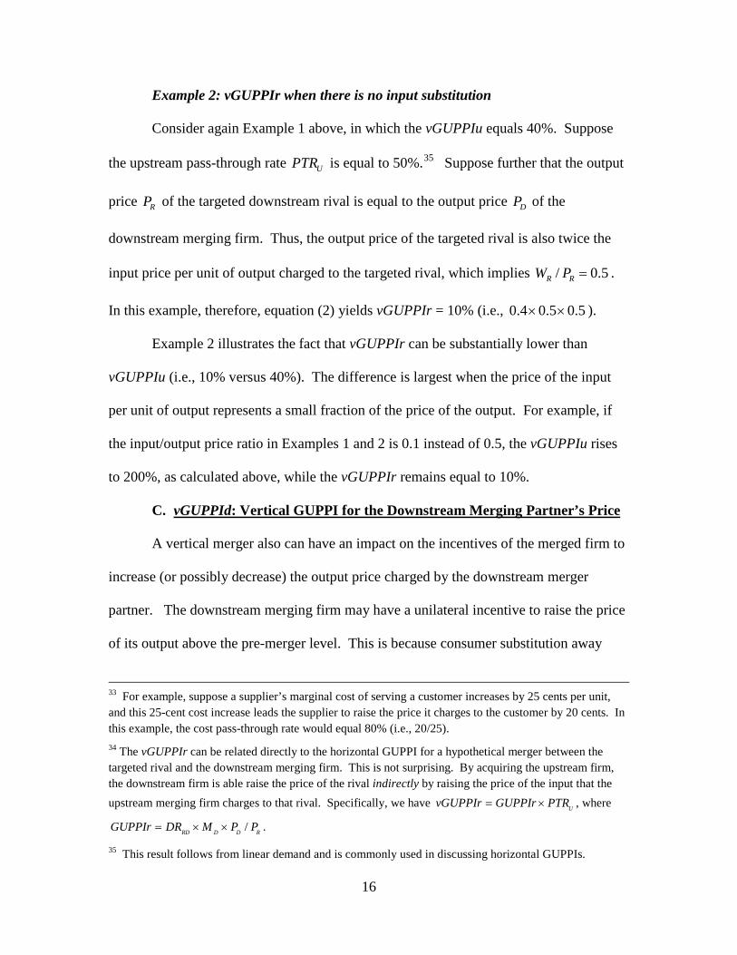
Example 2: vGUPPIr when there is no input substitution
Consider again Example 1 above, in which the vGUPPIu equals 40%. Suppose
the upstream pass-through rate UPTR is equal to 50%.35 Suppose further that the output
price RP of the targeted downstream rival is equal to the output price DP of the
downstream merging firm. Thus, the output price of the targeted rival is also twice the
input price per unit of output charged to the targeted rival, which implies / 0.5R RW P = .
In this example, therefore, equation (2) yields vGUPPIr = 10% (i.e., 0.4 0.5 0.5× × ).
Example 2 illustrates the fact that vGUPPIr can be substantially lower than
vGUPPIu (i.e., 10% versus 40%). The difference is largest when the price of the input
per unit of output represents a small fraction of the price of the output. For example, if
the input/output price ratio in Examples 1 and 2 is 0.1 instead of 0.5, the vGUPPIu rises
to 200%, as calculated above, while the vGUPPIr remains equal to 10%.
C. vGUPPId: Vertical GUPPI for the Downstream Merging Partner’s Price
A vertical merger also can have an impact on the incentives of the merged firm to
increase (or possibly decrease) the output price charged by the downstream merger
partner. The downstream merging firm may have a unilateral incentive to raise the price
of its output above the pre-merger level. This is because consumer substitution away
33 For example, suppose a supplier’s marginal cost of serving a customer increases by 25 cents per unit, and this 25-cent cost increase leads the supplier to raise the price it charges to the customer by 20 cents. In this example, the cost pass-through rate would equal 80% (i.e., 20/25). 34 The vGUPPIr can be related directly to the horizontal GUPPI for a hypothetical merger between the targeted rival and the downstream merging firm. This is not surprising. By acquiring the upstream firm, the downstream firm is able raise the price of the rival indirectly by raising the price of the input that the upstream merging firm charges to that rival. Specifically, we have UvGUPPIr GUPPIr PTR= × , where
/RD D D RGUPPIr DR M P P= × × . 35 This result follows from linear demand and is commonly used in discussing horizontal GUPPIs.

17
from the firm to rivals increases the input sales that the upstream merger partner makes to
rivals, which tends to increase the profits of the upstream merger partner. This upward
pricing pressure is the only downstream incentive effect if the downstream merging firm
does not use the input produced by the upstream merger partner. In this case, the
incremental profits of the upstream merger partner (resulting from the incremental input
sales to downstream rivals) give the downstream firm an incentive to raise price that it
does not have absent the merger.
However, if the downstream merging firm also uses the input of the upstream
merger partner, then the downstream firm also may have a unilateral incentive to reduce
its output price below the pre-merger level. This is the EDM effect. An output
expansion by the downstream firm increases the input sales that the upstream firm makes
to the downstream firm, which tends to increase the profits of the upstream firm.
We first consider a scenario that does not reckon EDM into the vGUPPId. This
scenario is appropriate when EDM is not found to be merger-specific.36 We refer to the
vGUPPI measure for this scenario as vGUPPId1. Following again the GUPPI
methodology described in the 2010 Merger Guidelines, we calculate vGUPPId1 as
follows:
value of sales diverted to upstream merging partnervGUPPId1revenue on volume lost by downstream merging partner
=
The vGUPPId1 is a positive number that can be written as:
/DU U U DvGUPPId1 DR M W P= × × (3)
36 Supra note 7.

18
where DUDR denotes the vertical diversion ratio from the downstream merging firm to
the upstream merger partner, UW and UM denote the upstream merging firm’s price and
percentage profit margin (on average across all the customers of the upstream merging
firm, excluding the downstream merger partner), and DP denotes the downstream merger
partner’s output price.
The vertical diversion ratio DUDR can be related to the horizontal diversion ratios
from the downstream merging firm to its rivals. For example, if all the rivals of the
downstream merging firm purchase the input sold by the upstream merger partner (and
one unit of output requires one unit of that input), then DUDR is equal to the “market
recapture rate” (or “aggregate diversion ratio”) following a unilateral price increase by
the downstream merging firm.37 This can be illustrated with the following example.
Example 3: vGUPPId when there is no EDM
Suppose the downstream merging firm unilaterally raises the price of its output
and, as a result, its unit sales fall by 100 units. Suppose further that the market recapture
rate is 75% so that the other downstream firms capture 75 out of those 100 units.
Suppose also that one-third of those 75 units (i.e., 25 units) require the input of the
upstream merging firm. Thus, the diversion ratio from the downstream merging firm to
the upstream merger partner is 25%DUDR = . Suppose the upstream merging firm earns
a margin MU of 50% on input sales to rivals of the downstream merger partner and the
37 The market recapture rate is the fraction of the output lost by the downstream merging firm that would be recaptured by all the other output manufacturers (including the targeted rivals). The 2010 Merger Guidelines use the market recapture rate in the context of market definition. Guidelines §4.1.3.

19
input price per unit of output is half the output price of the downstream merger partner,
i.e., WU /PD= 0.50. From equation (3), vGUPPId1 = 6.25% (i.e. 0.25 x 0.50 x 0.50).
In this analysis, the input prices of the upstream merger partner are held constant
at the pre-merger level. Thus, vGUPPId1 scores the first-round incentive to raise the
output price of the downstream merging firm before any increase in the input price
charged to any targeted downstream rivals. Specifically, it does not take into account the
impact of raising rivals’ costs on the pricing incentives of the downstream merging firm.
The vGUPPId1 also does not take into account any potential downward pricing
pressure from merger-specific EDM. Accounting for EDM will reduce the vGUPPId and
possibly make it negative. Suppose that the downstream merging firm is unable to
substitute away from inputs purchased from rival suppliers with inputs from the upstream
merger partner. Even here, merger-specific EDM could reduce its marginal cost. This
leads to the following formula, which we denote as vGUPPId2:
/UD D DvGUPPId2 vGUPPId1 M W P= − × (4)
where vGUPPId1 is given in equation (3), and UDM and DW denote the margin and price
of the upstream merging firm on input sales to the downstream merging firm.
Equation (4) implies that if market demand is perfectly price inelastic and
downstream firms are symmetric, then vGUPPId2 = 0. This key result follows because a
price increase by the downstream merging firm has no effect on total market output
(since market elasticity is zero) and also no effect on the total input sales and profits of
the upstream merger partner (since the latter earns the same margin on sales to all the

20
downstream firms). Thus, the merger does not create any incentive for the downstream
merging firm to change the price of its output, i.e., vGUPPId2 = 0.38
In fact, if instead market demand is not perfectly inelastic (or if some downstream
firms are not customers of the upstream merging firm) and there is symmetry among the
customers of the upstream firm, then vGUPPId2 < 0 and there is a strict incentive for the
downstream firm to reduce its price. For example, consider again Example 3 where
vGUPPId1 = 6.25%. Suppose the upstream merging firm also earns a margin of 50% on
input sales to the downstream merging firm, and the input/output price ratio also equals
0.5 for the downstream firm. Then, vGUPPId2 = -18.75% (i.e., 0.0625 0.5 0.5− × ). This
is because a price reduction by the downstream merging firm expands output and
increases its input purchases from the upstream merger partner by more than it reduces
the rivals’ input purchases. Therefore, in this case, the merger on balance creates
downward pricing pressure on the downstream merging firm.
In short, merger-specific EDM can make a substantial difference to the analysis,
even if there is no potential for input substitution.39 If vGUPPId <0, it will mitigate the
impact of vGUPPIr>0 and lead to a lower likelihood of significant adverse effects. The
first-round net incentive effect on downstream prices then could be gauged by calculating
a weighted average of vGUPPIr and vGUPPId.
D. Multiple Targeted Downstream Rivals
The vGUPPIu and vGUPPIr analyzed above evaluated the merged firm’s
incentives to raise the input prices charged to downstream rivals “one at a time.” That is,
38 Formally, zero market elasticity and symmetry imply 1DUDR = , U DW W= and U UDM M= . Equations
(3) and (4) then imply vGUPPId2 = 0. 39 Input substitution is discussed in Section III.
21
for each targeted downstream competitor, the vGUPPIu formula was derived holding the
input prices charged to other targeted competitors constant at their pre-merger level. This
is a conservative approach because the incentive to raise the input price to any given
targeted rival is higher if the merged firm simultaneously raises price also to other rivals.
This is an important issue because the merged firm may have the incentive to
foreclose multiple firms simultaneously, which can significantly increase the profitability
and the incentives to raise input prices further. Relying solely on the vGUPPIu (or the
vGUPPIr) calculated for a targeted price increase to a single rival can ignore significant
interaction effects from simultaneous price increases and, therefore, lead to significant
under-prediction of adverse effects.40
The vGUPPIu and vGUPPIr formulae can be extended to account for these
interaction effects. When the merged firm raises the input price to multiple downstream
rivals, there is more diversion to the downstream merger partner (than when it raises the
input price to just one rival). For example, suppose that the upstream firm were to raise
the input prices simultaneously to all its downstream rivals. If so, then a greater
percentage of the sales lost by each rival would be diverted to the downstream merger
partner because the downstream merger partner would be the only firm that did not
experience a price increase. This analysis can be illustrated with the following example.
40 The same issue arises in horizontal merger cases involving multi-product firms, if the GUPPIs for the multiple products sold by one merging firm are calculated separately for each product and one at a time. It is noteworthy that the Guidelines seem to instruct practitioners to evaluate the upward pricing pressure for each individual product separately. Guidelines §6.1 (“Adverse unilateral price effects can arise when the merger gives the merged entity an incentive to raise the price of a product previously sold by one merging firm and thereby divert sales to products previously sold by the other merging firm, boosting the profits on the latter products.”) (emphasis added) However, the Guidelines do not indicate whether the upward pricing pressure for each individual product sold by the same merging firm should be evaluated one at a time or simultaneously (i.e., whether the other prices charged by that firm should be held constant at their pre-merger level or should be assumed to rise as well).

22
Example 4: Simultaneously targeting multiple downstream rivals
Consider again Examples 1 and 2 above in which the diversion ratio between the
targeted downstream rival and the downstream merger partner was equal to 40%. That is,
if the merged firm raises the input price to that rival only, the downstream merger partner
captures 40% of the output that the rival loses as the result of the input price increase.
Given the margin and price data in these examples, the vGUPPIu and vGUPPIr were
40% and 10%, respectively. Suppose there is an identical second rival that also
purchases the input of the upstream merging firm and thus also can be targeted for input
foreclosure by the merged firm. One conservatively could apply the same vGUPPIs of
40% and 10% to the second targeted rival as well. However, if the merged firm raises the
input price to both rivals simultaneously, suppose the downstream merger partner would
capture 50% of the sales lost by the two rivals.41 This increase in the diversion ratio from
40% to 50% leads to an increase in the vGUPPIu from 40% to 50% and a corresponding
increase in the vGUPPIr from 10% to 12.5%.
41 This is consistent with a 20% diversion ratio between the two targeted rivals. As a general matter, if all the targeted downstream rivals are symmetric, so that the input price increases would be the same for each targeted rival and each targeted rival would have the same incentive to raise its own price, and if the downstream firms face linear demand, then the vGUPPIu and vGUPPIr can be calculated by replacing the standard diversion ratio RDDR for a single targeted rival (calculated holding the prices of other targeted
rivals constant) with the “overall” diversion ratio /(1 )RD RD RRDR DR DR∗ = − , where RRDR denotes the
aggregate diversion ratio from a targeted rival to all the other targeted rivals (following a unilateral price increase by a targeted rival). For example, suppose there are 3 targeted rivals and, if any one of them were to raise price unilaterally and lose 100 units of sales, then the downstream merging firm would capture 30 units (i.e., 30%RDDR = ) and each of the other 2 targeted rivals would capture 20 units (i.e., 40%RRDR = ).
(The remaining 30 units would be diverted to non-targeted rivals and outside goods.) With linear demand, if all 3 targeted rivals simultaneously raise price equally, then each of them loses 100 units “initially” and then recaptures 40 units when the other 2 targeted rivals also raise price. Thus, the 3 targeted rivals lose a total of 180 units when they raise price simultaneously. The downstream merging firm captures 90 units (i.e., 30 units from each targeted rival) and thus the overall diversion ratio equals 50% (i.e., 90/180). That
is, /(1 ) 0.3 /(1 0.4) 0.5RD RD RRDR DR DR∗ = − = − = .

23
III. Accounting for Input Substitution
The basic analysis above assumed that there is no ability for downstream rivals to
substitute away from the input sold by the upstream merging firm if it raises its price. As
a result, the only constraint on the upstream firm’s incentive to raise prices is the fact that
higher input prices will lead to higher output prices, which will choke off demand for the
products of the targeted firms and the inputs that they require. The lack of input
substitution also limited the magnitude of potential EDM.
The analysis changes when there is a potential for input substitution.42 When
downstream firms have access to production technologies that permit them to substitute
away from the input of the upstream merging firm to other suppliers, the market power of
the upstream merging firm will be lessened, both before and after the merger. This
substitution will mitigate (or possibly even eliminate) the cost increase and the associated
increase in the price of the targeted firm’s output. As a result, diversion to the
downstream merging firm from the input price increase also will be reduced. These
effects will reduce the incentive to engage in input foreclosure, perhaps very
substantially. This input substitution can be reckoned into the vGUPPI analysis.
A. vGUPPIu
In the presence of input substitution, the vGUPPIu formula is given as follows:
/1 /
RD D D R
R SR P
DR M P WvGUPPIuM E E× ×
=+ ×
(5)
The numerator in equation (5) is the vGUPPIu in the absence of input
substitution, and the denominator is the adjustment to be made to account for input
substitution. Since the denominator exceeds unity, input substitution tends to reduce the 42 Formal analysis is provided in the Appendix.

24
vGUPPIu (all else equal). The magnitude of the denominator—and the incentive to raise
the input price to the targeted rival—depends on two elasticities, SRE and Ep.43 SRE
measures the extent to which the targeted rival can substitute away from the upstream
merging firm’s input to other input suppliers.44 PE measures the extent to which the
targeted rival passes through an increase in the upstream merging firm’s input price into
its output price).45
Example 5: vGUPPIu when there is input substitution
Consider again the assumptions of Example 1. If there is no input substitution
( 0RES = ), the vGUPPIu equals 40% (i.e., the numerator in equation (5) equals 40%).
Suppose instead that there is input substitution and assume 2.5SRE = , 0.25PE = and
50%RM = . Thus, the denominator in equation (5) equals 6 (i.e., 1 0.5 2.5 / 0.25+ × ). It
follows that input substitution reduces the vGUPPIu from 40% to about 6.7% (i.e., 40%
divided by 6). This shows the large impact that input substitution can have on the
incentive to raise post-merger input prices.
43 We will discuss the estimation and the properties of these elasticities in Section III.D below.
44 We use URS to denote the upstream merging firm’s share of the targeted rival’s total purchases of the
relevant input. This share pertains to the relevant inputs under consideration (e.g., chemical products used as catalysts) and ignores all other types of inputs (e.g., other chemicals, labor and fuel). SRE denotes the
elasticity of URS with respect to an increase in the input price RW that the upstream merging firm charges to
the rival. For example, suppose a supplier raises the price of its input to a manufacturer by 10% and, as a result of the input price increase, the supplier’s share of the manufacturer’s total input purchases falls by 25%, say from 60% to 45%. In this example, SRE would equal 2.5 (i.e., 25% divided by 10%).
45 PE denotes the elasticity of the price of the targeted rival ( RP ) with respect to an increase in the input
price that the rival must pay to the upstream merging firm ( RW ). For example, suppose a supplier raises the
price of its input to a manufacturer by 10% and, as a result of the input price increase, the manufacturer raises the price of its output by 2.5%. In this example, PE would equal 0.25 (i.e., 2.5% divided by 10%).

25
Despite the additional complexity created by input substitution, the signs of the
various terms in equation (5) make intuitive sense. A higher value of SRE implies that the
targeted rival will substitute a larger share of inputs previously purchased from the
upstream merging firm with purchases from other suppliers (as opposed to raising its
output price) and thus implies that the merged firm will have a weaker incentive to raise
the input price to the targeted rival. Conversely, a higher value of PE implies that the
targeted rival will have an increased propensity to pass through an input price increase in
its output price (as opposed to substituting input purchases from the upstream merging
firm with input purchases from other suppliers) and thus implies that the merged firm will
have a stronger incentive to raise the input price to the targeted rival. Finally, a higher
value of RM implies that the targeted rival faces a more inelastic demand and, therefore,
the targeted rival loses fewer sales when it raises its output price in response to an input
price increase. This in turn implies that the volume of sales diverted from the foreclosed
rival to the merger partner is smaller, and hence the merged firm will have a weaker
incentive to raise the input price to the targeted downstream rival.
B. vGUPPIr
When there is input substitution, the vGUPPIr formula is given as follows:
post
URRU
R UR
SWvGUPPIr vGUPPIu PTRP S
= × × × (6)
where vGUPPIu is given in equation (5) and:
1post
URU SR
UR
S vGUPPIu PTR ES
= − × × (7)

26
These two equations show that input substitution has two effects that tend to
reduce the vGUPPIr. First, as indicated by equation (7), the fraction /postUR URS S is smaller
than unity and accounts for the fact that the targeted rival would respond to an increase in
the input price by reducing the share of its input purchases from the upstream merging
firm. Second, the value of vGUPPIu in equation (6) is smaller when there is input
substitution, which accounts for the fact that the input price increase by the upstream
merging firm would be smaller to begin with.
Example 6: vGUPPIr when there is input substitution
Consider again Example 5 where input substitution reduces vGUPPIu from 40%
to about 6.7%. From equation (7), input substitution also reduces the fraction /postUR URS S
from 1 to 0.917 (since 0.067 0.5 2.5 0.083U SRvGUPPIu PTR E× × = × × = ). It then
follows from equation (6) that input substitution reduces vGUPPIr from 10% to about
1.5% (i.e., 0.067 0.5 0.5 0.917× × × ).
C. vGUPPId3
If EDM is merger-specific and cognizable and the downstream merging firm also
has some ability to substitute inputs from rival suppliers with inputs from the upstream
merger partner, then the vGUPPId formula is given as follows:
22 ( ) /SD UD D DvGUPPId3 vGUPPId E M W P= − × × (8)
where vGUPPId2 is given in equation (4) and SDE denotes the pre-merger elasticity of the
upstream merging firm’s share of the downstream merging firm’s input purchases with
respect to the price that the upstream firm charges to the downstream firm. As shown by
equation (8), vGUPPId3 is lower than vGUPPId2. The input substitution further reduces
the upward pricing pressure and more likely will result in downward pricing pressure.

27
Example 7: vGUPPId when there is EDM and input substitution
Consider again Example 3 where, in the absence of EDM and input substitution,
vGUPPId1 is equal to 6.25%. Assuming that the upstream merging firm earns a margin
of 50% on input sales to the downstream merging firm, i.e., 50%UDM = , and that the
input price per unit of output is half the output price of the downstream merging firm, i.e.,
/ 0.5D DW P = , we found vGUPPId2 = -18.75%. Thus, in this illustrative example,
accounting for cognizable EDM was sufficient to turn a positive vGUPPId1 into a
negative vGUPPId2. If we also account for input substitution by the downstream
merging firm, the EDM effect becomes even stronger. To illustrate, suppose that the
downstream merging firm has the same ability as the targeted rival to substitute inputs
between the upstream merging firm and other suppliers, i.e., 2.5SDE = . Then, equation
(8) implies 3 50%vGUPPId = − (i.e., 218.75 2.5 0.5 0.5− − × × ).
D. Data Requirements and Calibration
In order to calculate the vGUPPIs when there is no input substitution, it is
necessary to have information similar to what is needed to calculate standard horizontal
GUPPIs. These data include the margins and prices of the upstream merging firm and the
downstream firms, as well as the diversion ratios among the downstream firms. In
addition, the analyst requires an estimate of the cost pass-through rate of the upstream
merging firm.
Certain variables might need to be estimated. To account for potential input
substitution between the input of the upstream merging firm and other suppliers of the
relevant input, it is necessary to estimate the elasticities SRE and PE for each targeted
rival. In addition, it is necessary to estimate the elasticity SDE for the downstream

28
merging firm to account for merger-specific EDM resulting from input substitution.
These elasticities might be estimated from data in public or proprietary documents from
the merging firms or from natural experiments.
These elasticities also may be inferred from other variables and the assumption of
profit-maximization.46 In particular, if one assumes for simplicity that downstream firms
are symmetric, then profit-maximization by the upstream merging firm implies:
1/SR SD U PE E M E E= = − × (9)
where E denotes the elasticity of downstream market demand with respect to an increase
in the downstream market price. If an estimate of the market elasticity E is available,
then equation (9) can be used together with an estimate of the input price pass-through
elasticity PE to “calibrate” the values of SRE and SDE . If instead an estimate of E is not
available, one can assume 1E = , and if an estimate of PE is not available then one can
use the approximation:47
/P R R RE PTR W P= × (10)
where RPTR is the standard cost pass-through rate that applies when a downstream firm
incurs an increase in its marginal cost of production (and does not expect any changes in
46 See, e.g., Joe Farrell & Carl Shapiro, Improving Critical Loss Analysis, ANTITRUST SOURCE, Feb. 2008, available at http://www.americanbar.org/content/dam/aba/publishing/antitrust_source/ index_1.authcheckdam.pdf.
47 By definition, ( / ) /P R R R R RE PTR C W W P= × ∆ ∆ × . Equation (10) thus might overstate the value of PE
because it implicitly assumes that / 1R RC W∆ ∆ = . This assumption is correct when there is no input
substitution.

29
its competitors’ prices).48
Example 8: Calibrating the values of SRE and SDE
Assuming that 0.5RPTR = and / 0.5R RW P = , then equation (10) implies that
0.25PE = (i.e., 0.5 0.5× ). Assuming a 50% margin and a market elasticity of 1 (i.e.,
50%UM = and 1E = ), equation (9) implies 1.75SR SDE E= = (i.e., 1/ 0.5 1 0.25− × ).
IV. Further Policy Analysis
Implementation of the vGUPPI methodology by the agencies would involve
several additional policy decisions. First, it would need to decide whether to focus on the
vGUPPIu or the vGUPPIr. Second, it would want to decide whether or not to apply a
safe harbor, and if so, at what level.
A. vGUPPIu versus vGUPPIr
In horizontal mergers, there is a GUPPI for each product sold by the merging
firms. We have calculated three basic vGUPPIs, one for the output price of the
downstream merging firm (vGUPPId), one for the input price charged by the upstream
merging firm to a rival of the downstream merging firm (vGUPPIu), and one for the
output price of the downstream rival targeted for the input price increase (vGUPPIr).
While it is clear that vGUPPId should be used to score the merger impact on the pricing
incentives of the downstream merging firm, there could be a policy debate about
48 When there are multiple targeted downstream rivals, the elasticity PE also could be higher as well as the
diversion ratio (see Section II.D). This depends on whether each targeted rival expects that the other targeted rivals also will face an input price increase and raise their prices as a result. The simpler approach would hold the beliefs and strategies of all non-merging firms (including the targeted downstream firms) constant and thus the same as their pre-merger beliefs and strategies, which would not lead to a higher PE .
This is the approach used for horizontal GUPPIs and therefore the most straightforward extension of the GUPPI methodology to vertical mergers.

30
vGUPPIu and vGUPPIr. Competitive effects analysis (and any safe harbor or
anticompetitive presumptions) could be based on the vGUPPIr of the targeted
downstream rival instead of, or in addition to, the vGUPPIu of the upstream firm.
In our view, there is a good policy rationale to prefer the use of the vGUPPIr
instead of vGUPPIu. The vGUPPIr is more relevant to gauging harm to the consumers
that purchase the downstream product. Even if the vGUPPIu is large, the input may be
sufficiently unimportant that it would not lead to significant effects downstream.
However, there are arguments that it would be inappropriate to eliminate a policy role for
vGUPPIu. It might be argued that harm to the downstream targeted rivals is or should be
sufficient harm to be cognizable. That is, these targeted downstream rivals also might be
“consumers” for the purposes of vertical merger enforcement.
There are competing doctrinal threads here. On the one hand, Aspen Ski makes it
clear that it is necessary to show consumer harm, not simply harm to a rival.49 Vertical
restraints cases like Jefferson Parish that allege exclusionary effects from exclusive
dealing are treated similarly.50 However, on the other hand, the 2010 Merger Guidelines
take the approach that it is not necessary to show adverse effects on consumers in
downstream markets for mergers of competing buyers that raise buy-side competitive
concerns.51 It appears that the Agencies intend that harm to the sellers would be
49 Aspen Skiing Co. v. Aspen Highlands Skiing Corp., 472 U.S. 585, 608-09 (1985). See also Krattenmaker & Salop, supra note 3. 50 Jefferson Parish Hosp. Dist. No. 2 v. Hyde, 466 U.S. 2 (1984) (applying rule of reason to exclusive dealing); United States v. Dentsply, Int’l, Inc. 399 F.3d. 181 (3d Cir. 2005). 51 Guidelines §12 (“Nor do the Agencies evaluate the competitive effects of mergers between competing buyers strictly, or even primarily on the basis of effects in the downstream markets in which the merging firms sell.”) This analysis seems to assume no merger efficiencies. If there are efficiencies, then there could be a trade-off between harm to the sellers and benefits to consumers. See Steven C. Salop & Serge Moresi, Updating the Merger Guidelines: Comments (Public Comment to Horizontal Merger Guidelines

31
sufficient to render the merger anticompetitive. Thus, this remains a policy issue for any
revision of the U.S. Vertical Merger Guidelines.
B. Safe Harbors
In light of the numerous policy issues raised in this article, it is premature for us
to recommend specific vGUPPI levels for use in a preliminary safe harbor, or indeed
whether to implement safe harbors.52 Instead, we merely will highlight a number of
discussion issues that will be relevant in making that determination. First, there is the
issue of whether to specify the safe harbor in terms of the vGUPPIr or the vGUPPIu.
The vGUPPIu better predicts the harm to the downstream competitors who are customers
of the upstream merging firm. However, harms to the customers of the downstream
competitors are better predicted by the vGUPPIr.
Second, there is the issue of whether to specify safe harbors based on the simplest
vGUPPIs derived for an input price increase that targets a single rival, or whether to take
into account the potential or likelihood of multi-rival targeting of post-merger input price
increases. The latter clearly predicts a greater incentive to foreclose.53
Third, there is the issue of which vGUPPId to specify for the safe harbor. The
most restrictive approach would be to use vGUPPId1 where it is not clear whether EDM
Review Project Nov. 2009), available at http://www.ftc.gov/os/comments/horizontalmergerguides/545095-00032.pdf. 52 The 2010 Merger Guidelines suggest a horizontal GUPPI safe harbor when “the value of diverted sales is proportionately small.” 2010 Merger Guidelines, supra note 10 at §6.1. A subsequent speech by then-deputy AAG Carl Shapiro explicitly specified the safe harbor level as a GUPPI less than 5%. Carl Shapiro, Update from the Antitrust Division: Remarks to the Antitrust Law Fall Forum (November 18, 2010) at 24. (“Put differently, unilateral price effects for a given product are unlikely if the gross upward pricing pressure index for that product is less than 5%.”) This GUPPI safe harbor presumably is premised on a certain level of presumed efficiency benefits, along with other competitive effects factors and uncertainty. 53 See supra Section II.D.

32
will be a cognizable efficiency benefit, but use the vGUPPId2 or vGUPPId3 where it
likely would be cognizable.
Fourth, there is the issue of whether to reduce the data requirements of an initial
screen by relying on assumed values for the pass-through rate UPTR and assuming no
input substitution, as set out in Section II. For example, one simple approach would be to
assume 50%UPTR = and assume further that there is no input substitution or EDM.54 It
might be argued that basing the safe harbor on no EDM or input substitution could lead to
an overly intrusive standard. The argument on the other side is that a safe harbor is
intended to be narrow. Moreover, the actual value of UPTR might be expected
sometimes to exceed the default level of 50%. Finally, concerns about over- or under-
intrusiveness also can be eliminated by changing the safe harbor level rather than the
assumptions on which it is based.
V. Comparing vGUPPIu to the Vertical Arithmetic Methodology
“Vertical arithmetic” is another methodology that has been used to score
foreclosure incentives in vertical mergers.55 The vGUPPIs and vertical arithmetic have
similar goals and the calculations share a common approach. In fact, the vertical
arithmetic can be expressed as a vGUPPIu test with a specific safe harbor.
However, there are several differences. First, the vertical arithmetic gauges only
the likelihood of withholding the input. Unlike the vGUPPIs, it does not gauge the
54 The assumption of 50%UPTR = is consistent with linear demand functions in the downstream output
market and fixed-proportion demand functions in the upstream input market. With variable proportions, the upstream cost pass-through rate UPTR can be smaller than 50% (e.g., if downstream demand functions
are linear). 55 Vertical arithmetic calculations have been carried out for a number of vertical mergers and joint ventures. See supra note 14.
33
impact on prices paid by consumers in the downstream market. Second, and related, the
vertical arithmetic does not take into account the impact of EDM, whereas the vGUPPId
does. Third, the vertical arithmetic evaluates the incentive for non-price rationing
through a partial or total refusal to deal, whereas the vGUPPIs evaluate pricing
incentives.
For mergers in markets where the input price is fixed at a regulated level, the
vertical arithmetic can be used to evaluate the incentives for non-price exclusion (i.e.,
denying, delaying or degrading access) from a facility that is used as an input by
downstream competitors and is controlled by the upstream merging partner. For
example, it would apply to telephony mergers where the price of access to the local ILEC
network is regulated. However, in markets where input prices are not regulated but are
set by the upstream merging firms, the vGUPPIu has advantages, even aside from EDM
or gauging downstream effects. Increasing input prices is generally a more profitable
way of rationing demand than is withholding input sales at a constant price. This greater
profitability normally leads to a greater incentive to foreclose.56
The relationship of the incentives for non-price rationing expressed by the vertical
arithmetic methodology and the pricing incentives expressed by the vGUPPIu is
straightforward to explain. Suppose the upstream merging firm were to withhold one unit
of the input from a targeted rival of the downstream merger partner, but maintain the
same input price for the remaining units sold. In that case, the upstream firm’s profits
would be reduced by its dollar incremental profit margin U RM W . Faced with this loss of
a unit of the input, the targeted downstream rival would attempt to substitute to other 56 In the case of non-price foreclosure that must be lumpy (e.g., all or nothing refusals to deal or discrete quality degradation), non-price foreclosure could end up being more severe than price foreclosure.

34
possibly less efficient or more costly inputs. Either way, it might also have the incentive
to raise its price. As a result, the downstream rival likely would lose some sales to other
downstream firms, including the downstream merger partner. In the simplest vertical
arithmetic scenario, it is assumed that these other downstream firms do not raise their
prices, but simply absorb the sales diverted to them at their original prices.57
Suppose that the input is used in fixed proportions, for example, one unit of input
for each unit of output. Suppose that in response to the withholding of one unit of the
input by the upstream merging firm, the downstream merging firm obtains a fraction
UDDR of a unit of additional sales. Suppose that it earns a dollar profit margin D DM P on
each of these sales and, therefore, incremental profits of UD D DDR M P .
The other downstream firms also obtain additional sales (except of course the
foreclosed rival). Those firms also may use the input supplied by the upstream merging
firm, and they will purchase more of it as their sales expand post-foreclosure. This
diversion to the downstream merging firm and the non-targeted rivals in turn allows the
upstream merging firm to recapture a fraction F of the withheld unit from sales to other
firms, including the downstream merging firm.58 Thus, assuming that the upstream
57 The same assumption also applies to vGUPPIu. 58 Assuming fixed proportions (i.e., each downstream firm purchases one unit of the upstream merging firm’s input for each unit of output produced), RF R= , where RR is the aggregate diversion ratio, that is,
the fraction of the sales lost by the targeted rival that are diverted to the downstream merging firm and the other non-targeted rivals in the market, following a unilateral price increase by the targeted rival. If one assumes that the downstream firms have the same aggregate diversion ratio ( R ) to their competitors, then 1F R ME= = − , where E is the downstream market elasticity and M is the average margin of the downstream firms. See Serge Moresi, Diversion Ratios and Market Elasticity: Some Useful Formulas, unpublished paper (2011), available at http://crai.com/uploadedFiles/RELATING_MATERIALS/ Publications/LAE/Antitrust_and_Competition_Economics/Diversion_Ratios_and_Market_Elasticity_Some_Useful_Formulas.pdf.

35
merging firm earns the same dollar margin from all its customers, the net loss in margin
of the upstream merging firm is equal to (1 ) U RF M W− .
Comparing the profit gains by the downstream merging partner to the profit losses
by the upstream merging partner, the withholding would be profitable on balance, if and
only if:
(1 )UD D D U RDR M P F M W> − (11)
This can be rewritten in terms of the vGUPPIu. Using equation (1), withholding
one unit of input would be profitable if and only if:
(1 ) UvGUPPIu F M> − (12)
For example, suppose that 15%vGUPPIu = and (1 ) 20%UF M− = , so that
equation (9) would not be satisfied. In this case, vertical arithmetic would lead to the
conclusion that (non-price) foreclosure is not profitable. In contrast, if the input price is
not regulated, the vGUPPIu of 15% would indicate that it is profitable for the merged
firm to raise the input price. This difference in the profitability conditions flows from the
fact that when the input price is raised, the customer pays a higher price on all the units it
continues to purchase. However, the vertical arithmetic assumes that the merged firm
withholds input sales to a downstream rival but does not raise its price on the units that
the downstream rival continues to purchase. Thus, the withholding strategy of the
vertical arithmetic methodology is less profitable than is the price-increasing strategy of
the vGUPPIu.
One can view of the vertical arithmetic as a vGUPPIu test with an effective safe
harbor level set equal to (1 ) UF M− . This means that use of the vertical arithmetic could
lead to a more or less permissible policy, depending on the vGUPPIu safe harbor used by

36
the agency. For example, if 50%UM = and 60%F = , then the use of the vertical
arithmetic effectively would amount to a vGUPPIu safe harbor of 30%.
VI. Conclusions
This article has applied the basic GUPPI methodology to encompass pricing
incentives in vertical mergers. It has formulated vGUPPIs for scoring the merged firm’s
incentives to engage in input foreclosure and reduce output and explained how the
vGUPPIs relate to hypothetical partial equity transactions between the downstream
merging firm and its competitors. It also has analyzed several ways to take EDM into
account. The vGUPPIs thus can be used for the evaluation of vertical mergers in the
same way that standard GUPPIs are used for horizontal mergers.
This analysis of vGUPPIs is part of a larger project to design a menu of
“incentive scoring” methodologies for various competitive concerns raised in merger
policy. The standard GUPPIs can be used to score the incentives for unilateral price
increases in horizontal mergers. The basic GUPPI methodology can be extended for
firms that compete in quantities or capacity instead of price,59 bidding markets,60 and
markets with congestion issues.61 It also can be applied to acquisitions of partial
ownership interests.62
The vGUPPIs here are used to score the incentives for input foreclosure and
downstream unilateral price increases in vertical mergers. We (and our co-authors) have 59 Moresi, supra note 13. 60 Id. 61 Robert Willig, Unilateral Competitive Effects of Mergers: Upward Pricing Pressure, Product Quality, and Other Extensions, 39 REV. INDUS. ORG.19 (2011); Brijesh P. Pinto & David S. Sibley, Network Congestion and the Unilateral Effects Analysis of Mergers, unpublished manuscript (2012). 62 2010 Merger Guidelines §13; Daniel P. O’Brien & Steven C. Salop, Competitive Effects of Partial Ownership: Financial Interest and Corporate Control, 67 ANTITRUST L.J. 559 (2000).

37
previously designed an analogous coordination price pressure index (“CPPI”)
methodology to score the incentives and ability for leading firms in a market to engage in
parallel accommodating conduct in the context of horizontal mergers.63
The use of these incentive scoring methodologies represents a significant advance
in the economic evaluation of competitive effects analysis for mergers and joint ventures,
in particular in the early phase of an investigation. Antitrust analysis is premised on the
assumption that firms are rational, profit-maximizing entities. Thus, the economic
incentives of the firms provide relevant information about the likely outcomes of these
combinations. While incentive scoring is not the only information relevant for evaluating
likely effects, it clearly is useful evidence.
Incentive scoring methodologies are more informative than simple structural
measures such as the HHI or other concentration indices. The increase in the HHI
generally does not relate directly to the change in unilateral incentives caused by a
merger. As a matter of economic analysis, those concentration indices are particularly
relevant for some type of conduct but not others.64 Thus, economic analysis does not
support concentration having the primary predictive role ascribed to it in cases like
Philadelphia National Bank.65 This shortcoming of concentration as a predictor has now
been recognized in cases like Baker Hughes.66 Incentive scoring methodologies like the
GUPPI, vGUPPI and CPPI can help fill the gap.
63 Serge Moresi, David Reitman, Steve C. Salop & Yianis Sarafidis, Gauging Parallel Accommodating Conduct Concerns with the CPPI, unpublished manuscript (2011), available at http://papers.ssrn.com/sol3/papers.cfm?abstract_id=1924516). 64 Robert E. Dansby & Robert D. Willig, Industry Performance Gradient Indexes, 69 AM. ECON. REV. 249 ( 1979). 65 United States v. Philadelphia National Bank, 374 U.S. 321,362-63 (1963). 66 United States v. Baker Hughes, Inc., 908 F.2d 981, 984 (1990).

38
Additional incentive scoring methodologies also are needed. The vGUPPIu is
designed primarily to address input foreclosure concerns in vertical merger cases. A
somewhat different analysis likely is needed to evaluate the incentives to engage in
customer foreclosure. Similarly, the CPPI is designed to address coordinated price
increases through parallel accommodating conduct. A somewhat different analysis likely
is needed to evaluate the incentives to engage in collusive conduct that relies on detection
and punishment of defections from tacitly agreed-upon terms of coordination.67 We hope
that this article helps create further momentum to move antitrust analysis forward in this
direction.
67 Analysis of the incentives to engage in coordination also may differ if firms interact in multiple markets. See, e.g., B. Douglas Bernheim & Michael D. Whinston, Multimarket Contact and Collusive Behavior, 21 RAND J. ECON. 1 (1990).

39
Glossary
Firm-U, Firm-D, Firm-R: The upstream merging firm (U), the downstream merging firm (D) and the downstream rival (R) targeted for input foreclosing price increases.
Diversion Ratio UDDR : The fraction of Firm-U’s sales lost (when Firm-U raises its price) that are gained by Firm-D.
Diversion Ratio RDDR : The fraction of Firm-R’s sales lost (when Firm-R raises its price) that are gained by Firm-D.
Diversion Ratio DUDR : The fraction of Firm-D’s sales lost (when Firm-D raises its price) that are gained by Firm-U.
Upstream Prices RW and DW : Input prices charged by Firm-U to Firm-R and Firm-D, respectively.
Upstream Average Price UW : Average input price charged by Firm-U to all downstream firms, excluding Firm-D.
Downstream Prices DP and RP : Output prices charged by Firm-R and Firm-D, respectively.
Average Upstream Margin UM : Firm-U’s average variable profit margin (i.e., its
average price charged to all firms except Firm-D less its variable cost, U UW C− )
expressed as a percentage of its average price. That is, ( ) /U U U UM W C W= − .
Upstream Margin UDM : Firm-U’s variable profit margin on input sales to Firm-D.
Downstream Margin DM : Firm-D’s variable profit margin (i.e., its price less its variable
cost, D DP C− ) expressed as a percentage of its price. That is, ( ) /D D D DM P C P= − .
Downstream Margin RM : Firm-R’s variable profit margin (i.e., its price less its variable
cost, R RP C− ) expressed as a percentage of its price. That is, ( ) /R R R RM P C P= − .
Upstream Pass-Through Rate UPTR : The absolute (i.e., dollar) increase in the input
price charged to Firm-R ( RW∆ ) following an absolute increase in Firm-U’s marginal cost
of serving Firm-R ( UC∆ ), expressed as a percentage of the increase in marginal cost.
That is, /U R UPTR W C= ∆ ∆ .

40
Downstream Pass-Through Rate RPTR : The absolute (i.e., dollar) increase in the output
price charged by Firm-R ( RP∆ ) following an absolute increase in Firm-R’s marginal cost
of production ( RC∆ ), expressed as a percentage of the increase in marginal cost. That is,
/R R RPTR P C= ∆ ∆ .
Downstream Pass-Through Elasticity PE : The percentage increase in Firm-R’s output price caused by a one-percent increase in Firm-U’s input price charged to Firm-R. That is, ( / ) /( / )P R R R RE P P W W= ∆ ∆ . Equivalently, ( / ) /P R R R R RE PTR C W W P= × ∆ ∆ × .
Market Elasticity E : The percentage reduction in downstream market demand caused by a one-percent increase in the downstream market price.
Purchase Share URS : Firm-U’s share of Firm-R’s total purchases of the relevant input.
Purchase Share Ratio /postUR URS S : The ratio of Firm-U’s share of Firm-R’s input
purchases after the target price increase to the share before the input price increase.
Purchase Share Elasticities SRE and SDE : SRE is the elasticity of the purchase share URS
with respect to an increase in the input price RW that Firm-U charges to Firm-R.
Similarly, SDE is the elasticity of Firm-U’s share of the input purchases of Firm-D with
respect to an increase in the input price DW that Firm-U charges to Firm-D.

41
APPENDIX
A. The Technical Underpinnings of vGUPPI Analysis
The vGUPPIs can be derived from a formal economic model of upstream
competition among input suppliers and downstream competition among output
manufacturers.
1. Basic model with differentiated inputs and differentiated products
The formal model is a three-stage game involving N input suppliers and M output
manufacturers. In the first stage, the suppliers simultaneously set the prices of their
inputs and each supplier can set different prices to different manufacturers.68 In the
second stage, each manufacturer observes only the input prices at which it will be able to
purchase inputs from the suppliers; it does not observe the input prices that the suppliers
are charging the other manufacturers. The manufacturers then simultaneously set their
product prices. These prices determine the each manufacturer’s product demand, that is,
the orders that the manufacturer receives from its own customers. In the third stage, each
manufacturer chooses how many inputs to purchase from each supplier, given the volume
of orders received and the input prices set by the suppliers. Production and delivery then
occur, and the game ends.
We assume that each supplier and manufacturer chooses its price to maximize
profits,69 and that manufacturers also choose inputs to minimize their costs. The
68 We assume suppliers set linear prices and manufacturers have no bargaining power over input prices. 69 We assume no coordination both before and after the merger.

42
equilibrium concept considered in this analysis is perfect Bayesian equilibrium.70 We
thus analyze the model using backward induction.71
a. Manufacturers’ purchases of inputs
Each manufacturer faces a standard cost-minimization problem (in stage 3).
Specifically, manufacturer m must fulfill a given volume mQ of orders (that it received in
stage 2) and faces given input prices 1mW , 2
mW , …, NmW from supplier 1, supplier 2, …,
supplier N, respectively (that the suppliers set in stage 1). We assume that the
manufacturer must purchase from the N suppliers a total volume of inputs equal to m mA Q ,
that is, one unit of output of manufacturer m requires mA units of input.72 We further
assume that the manufacturer’s cost of production can be reduced by purchasing inputs
70 Because manufacturers do not observe the input prices offered to their competitors, each manufacturer must form beliefs about the input prices paid by other manufacturers. In equilibrium, those beliefs must be correct. In general, there are many perfect Bayesian equilibria because there are many different ways that beliefs can be specified following an unexpected (off equilibrium) input price offer. In this paper, we assume that each manufacturer has “passive beliefs” about the input prices offered to its competitors. This means that, when a supplier contemplates raising the price of its input to a given manufacturer, the supplier expects that the manufacturer will not change its beliefs with respect to the input prices that the supplier is offering to its competitors (and hence that the manufacturer also will not change its beliefs with respect to the output prices that its competitors will set in the downstream market). This assumption of passive beliefs affects the manufacturer’s response to an input price increase, and hence the equilibrium level of input prices. See Patrick Rey & Jean Tirole, A Primer on Foreclosure, in Mark Armstrong and Rob Porter, eds., III HANDBOOK INDUS. ORG. 2145 (2007) at § 2.1.2. 71 For a formal treatment of the concepts of perfect Bayesian equilibrium and backward induction, see, e.g., ROBERT GIBBONS, GAME THEORY FOR APPLIED ECONOMISTS (1992).
72 The value of the scale factor mA depends on the choice of units of measurement for the manufacturer’s
output and the relevant inputs purchased by the manufacturer. With no loss of generality, we will set the value of mA so that, at the pre-merger equilibrium, the manufacturer purchases from the upstream merging
firm a quantity of input equal to the manufacturer’s quantity of output. See also infra note 79.

43
from multiple suppliers, so that the manufacturer’s cost-minimization solution is to
purchase inputs from several of the N suppliers.73
1 2( , ,..., )j Nm m m mS W W W denotes supplier j’s share of the total volume of inputs
purchased (from the N suppliers) by manufacturer m. Thus, the volume of inputs
purchased by manufacturer m from supplier j is given by 1 2( , ,..., )j Nm m m m m mS W W W A Q . We
assume that the function jmS is decreasing in j
mW and increasing in kmW for k j≠ . That
is, supplier j will get a smaller share of the manufacturer’s input purchases if it raises the
price it charges the manufacturer for its input, and it will get a higher share if another
supplier raises its price. We use 1 2( , ,..., )Nm m m mC W W W to denote the marginal cost of
production of manufacturer m. We assume that the function mC is increasing in the input
prices 1 2( , ,..., )Nm m mW W W faced by manufacturer m. (The marginal cost of production mC
also includes the incremental costs of other types of inputs.) We assume that the
manufacturers’ production technologies exhibit constant returns to scale, and thus the
functions jmS and mC do not depend on the level of output ( mQ ).
b. Competition among manufacturers in the downstream market
Assuming a standard model of Bertrand competition with differentiated products,
manufacturer m takes the equilibrium prices charged by the other manufacturers as given
and chooses its price mP to maximize its profit,
( ) ( , )m m m m mP C D P P−− (A1)
73 We assume each manufacturer faces a cost-minimization problem similar to that in Roman Inderst & Tommaso Valletti, Incentives for input foreclosure, 55 EUR. ECON. REV. 820 (2011).

44
where mP− is the vector of equilibrium prices of all the other manufacturers and mD is the
demand function for the product sold by manufacturer m.74 The first-order condition
(FOC) for the price of manufacturer m to be profit-maximizing is:
( ) 0mm m m
m
DD P CP
∂+ − =
∂ (A2)
Solving this equation for mP , the equilibrium price strategy of manufacturer m is a
function of the manufacturer’s marginal cost, or ( )m mP C .75 Note that this pricing
strategy is actually a function of the input prices that suppliers charge to manufacturer m
since mC depends on those prices (see Section 1.a above). For this reason, we sometimes
write 1 2( , ,..., )Nm m m mP W W W instead of ( )m mP C .
c. Competition among suppliers in the upstream market
Consider input supplier n and the price niW that it charges to manufacturer i. In
equilibrium, supplier n sets niW to maximize its total profits holding all other prices
constant, except for the price of manufacturer i, i.e., iP .76 We thus write the profit
function of supplier n as:
( ) ( ) ( ( )) ( ) ( ( ))M
n n n n n n n n ni i i i i i i i k k k k k i i
k iW C S W A D P W W C S A D P W
≠
− + −∑ (A3)
where nkC is the marginal cost of supplier n of producing inputs for manufacturer k. This
profit function adds up all the profits that supplier n obtains from all the manufacturers. 74 We focus on vertical mergers where the upstream and downstream merging firms are not vertically integrated. See supra notes 9 and 12. 75 This function implicitly also depends on the equilibrium prices of the other manufacturers. See supra note 71. 76 The supplier takes the equilibrium prices charged by the other manufacturers as given because they do not observe the input price that the supplier is charging to the manufacturer under consideration.

45
The FOC for niW is:
( ) 0n
n n n i i ii i i i in n
i i i
D P SW C A S D other termsP W W
∂ ∂ ∂− + + = ∂ ∂ ∂
(A4)
The first term in (A4) is negative and represents the loss from reduced sales to
manufacturer i that supplier n would incur if it raised the price niW that it charges to
manufacturer i. Specifically, manufacturer i would reduce its purchases from supplier n
for two reasons. First, manufacturer i would increase the price of its product by the
amount / ni iP W∂ ∂ and this would lead to a reduction in its volume of sales equal to
( / )( / )ni i i iD P P W∂ ∂ ∂ ∂ . If manufacturer i were to hold supplier n’s share of its total input
purchases constant (i.e., if niS did not change), this would reduce supplier n’s input sales
to manufacturer i by the amount ( / )( / )n ni i i i i iA S D P P W∂ ∂ ∂ ∂ . Second, manufacturer i
actually would reduce niS by the amount /n n
i iS W∂ ∂ and this would lead to a further
reduction in supplier n’s input sales to manufacturer i equal to ( / )n ni i i iA D S W∂ ∂ .
The “other terms” in (A4) are positive and represent two sources of profit gains to
supplier n following an increase in the price charged to manufacturer i. First, supplier n
would be earning a higher margin on the volume of inputs that manufacturer i would
continue to purchase from supplier n. Second, supplier n would be selling larger volumes
of inputs to the other manufacturers because some of the customers of manufacturer i
would be switching to other manufacturers. To simplify the exposition, we do not show
these profit gains explicitly in (A4) and instead denote them as “other terms”. (These
other terms do not matter for the derivation of the vGUPPIs, as will be shown below.)

46
In (perfect Bayesian) equilibrium, (A4) and (A2) are satisfied for all input prices
and all output prices respectively.
2. Unilateral effects of a vertical merger on pricing incentives
We analyze the potential unilateral effects on pricing incentives from a vertical
merger of supplier 1 and manufacturer 1.
a. vGUPPIu for the upstream merging firm
The vertical merger of supplier 1 and manufacturer 1 can give supplier 1 a
unilateral incentive to raise the price of the input to manufacturer 2, a rival of the
downstream merger partner. A similar unilateral incentive exists for each downstream
rival that might be targeted with an input price increase.
The profit function of the merged firm is given by:
1 1 11 1 1 1 1 1 1
1( ) ( , ) ( ) ( , )
M
k k k k kk
P C D P P W C S A D P P− −=
− + −∑ (A5)
so that the post-merger FOC with respect to 12W can be written as:
1 21 1 1
2 2
11 1 1 2 2 2
2 2 2 2 21 12 2 2
( )
( ) 0
D PP CP W
D P SW C A S D other termsP W W
∂ ∂− +
∂ ∂
∂ ∂ ∂− + + = ∂ ∂ ∂
(A6)
This FOC says that post-merger the merged firm’s incentive to increase 12W must
be zero. Instead of solving for the equilibrium of the model, we follow the GUPPI
methodology and evaluate the merged firm’s incentive to increase 12W , beginning at the
pre-merger equilibrium. That is, we evaluate the left-hand side of (A6) at the pre-merger
equilibrium strategies. Therefore, in (A6), the downstream price of each manufacturer m
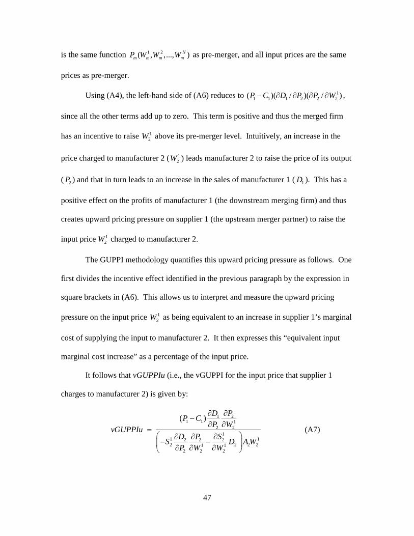
47
is the same function 1 2( , ,..., )Nm m m mP W W W as pre-merger, and all input prices are the same
prices as pre-merger.
Using (A4), the left-hand side of (A6) reduces to 11 1 1 2 2 2( )( / )( / )P C D P P W− ∂ ∂ ∂ ∂ ,
since all the other terms add up to zero. This term is positive and thus the merged firm
has an incentive to raise 12W above its pre-merger level. Intuitively, an increase in the
price charged to manufacturer 2 ( 12W ) leads manufacturer 2 to raise the price of its output
( 2P ) and that in turn leads to an increase in the sales of manufacturer 1 ( 1D ). This has a
positive effect on the profits of manufacturer 1 (the downstream merging firm) and thus
creates upward pricing pressure on supplier 1 (the upstream merger partner) to raise the
input price 12W charged to manufacturer 2.
The GUPPI methodology quantifies this upward pricing pressure as follows. One
first divides the incentive effect identified in the previous paragraph by the expression in
square brackets in (A6). This allows us to interpret and measure the upward pricing
pressure on the input price 12W as being equivalent to an increase in supplier 1’s marginal
cost of supplying the input to manufacturer 2. It then expresses this “equivalent input
marginal cost increase” as a percentage of the input price.
It follows that vGUPPIu (i.e., the vGUPPI for the input price that supplier 1
charges to manufacturer 2) is given by:
1 21 1 1
2 21
1 12 2 22 2 2 21 1
2 2 2
( ) D PP CP WvGUPPIu
D P SS D A WP W W
∂ ∂−
∂ ∂=
∂ ∂ ∂− − ∂ ∂ ∂
(A7)

48
This is the standard GUPPI ratio described in the 2010 Merger Guidelines. The
numerator is the “value of sales diverted” to the merger partner, that is, the profit gained
by manufacturer 1 following an increase in the input price charged to manufacturer 2.
The denominator is the “lost revenues attributable to the reduction in unit sales [to
manufacturer 2] resulting from the input price increase [to manufacturer 2]”.77
Dividing both the numerator and the denominator by 12 2 2 2( / )( / )D P P W− ∂ ∂ ∂ ∂ and
then using the FOC for 2P (i.e., 2 2 2 2 2/( / )P C D D P− = − ∂ ∂ ), one obtains:
21 1 11 1
2 2 2 2(1 / )SR P
DR M PvGUPPIuM E E S A W
=+
(A8)
where 21 1 2 2 2( / ) /( / )DR D P D P= − ∂ ∂ ∂ ∂ is the diversion ratio from manufacturer 2 to
manufacturer 1, ( ) /m m m mM P C P= − is the percentage profit margin of manufacturer m,
1 1 1 12 2 2 2( / )( / )SRE S W W S= − ∂ ∂ is the elasticity of supplier 1’s share of manufacturer 2’s total
input purchases with respect to an increase in the input price 12W charged by supplier 1 to
manufacturer 2, and 1 12 2 2 2( / )( / )PE P W W P= ∂ ∂ is the elasticity of the price of the output of
manufacturer 2 with respect to an increase in the input price 12W charged by supplier 1 to
manufacturer 2.78
Note that the vGUPPIu formula in (A8) depends on the pre-merger profit margin
( 1 1P C− ) of the downstream merger partner. This could suggest that a higher profit
77 2010 Merger Guidelines at §6.1. 78 Equations (1) and (5) in the main text are derived from (A8). With no loss of generality, we assume that
units of measurement are such that, at the pre-merger equilibrium, 1
2 2 1S A = , i.e., each targeted rival
purchases a quantity of input from the upstream merging firm equal to the quantity of output that it
produces. This simply means that the input price 1
2W must be calculated as the cost of the input purchased
from the upstream merging firm per unit of output produced by the targeted rival.
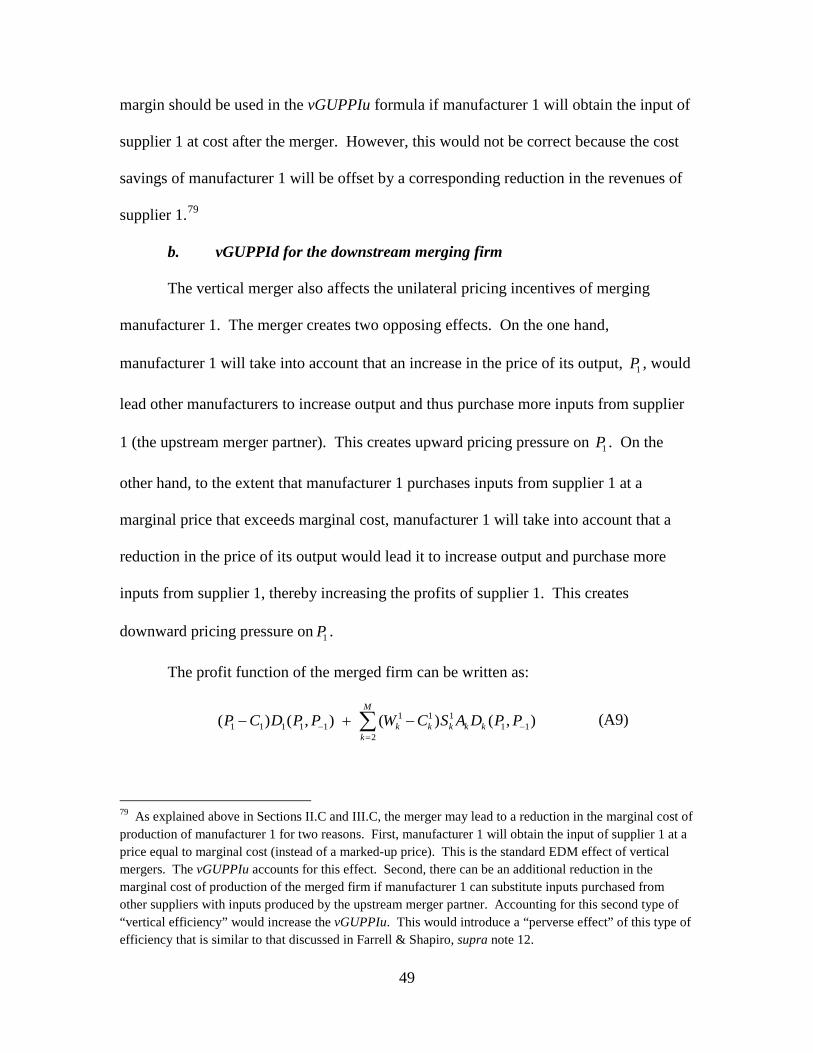
49
margin should be used in the vGUPPIu formula if manufacturer 1 will obtain the input of
supplier 1 at cost after the merger. However, this would not be correct because the cost
savings of manufacturer 1 will be offset by a corresponding reduction in the revenues of
supplier 1.79
b. vGUPPId for the downstream merging firm
The vertical merger also affects the unilateral pricing incentives of merging
manufacturer 1. The merger creates two opposing effects. On the one hand,
manufacturer 1 will take into account that an increase in the price of its output, 1P , would
lead other manufacturers to increase output and thus purchase more inputs from supplier
1 (the upstream merger partner). This creates upward pricing pressure on 1P . On the
other hand, to the extent that manufacturer 1 purchases inputs from supplier 1 at a
marginal price that exceeds marginal cost, manufacturer 1 will take into account that a
reduction in the price of its output would lead it to increase output and purchase more
inputs from supplier 1, thereby increasing the profits of supplier 1. This creates
downward pricing pressure on 1P .
The profit function of the merged firm can be written as:
1 1 11 1 1 1 1 1 1
2( ) ( , ) ( ) ( , )
M
k k k k kk
P C D P P W C S A D P P− −=
− + −∑ (A9)
79 As explained above in Sections II.C and III.C, the merger may lead to a reduction in the marginal cost of production of manufacturer 1 for two reasons. First, manufacturer 1 will obtain the input of supplier 1 at a price equal to marginal cost (instead of a marked-up price). This is the standard EDM effect of vertical mergers. The vGUPPIu accounts for this effect. Second, there can be an additional reduction in the marginal cost of production of the merged firm if manufacturer 1 can substitute inputs purchased from other suppliers with inputs produced by the upstream merger partner. Accounting for this second type of “vertical efficiency” would increase the vGUPPIu. This would introduce a “perverse effect” of this type of efficiency that is similar to that discussed in Farrell & Shapiro, supra note 12.

50
where 1 21 1 1 1 1( , ,..., )NC C C W W= is the post-merger marginal cost of manufacturer 1 since
supplier 1 will provide the input to manufacturer 1 at cost, i.e., 1 11 1W C= . For later use,
we denote by 1C∆ the post-merger reduction in the marginal cost of production of
manufacturer 1:
1 2 1 21 1 1 1 1 1 1 1 1( , ,..., ) ( , ,..., )N NC C W W W C C W W∆ = − (A10)
The first-order condition with respect to 1P reads:
1 1 111 1 1
21 1
( ) ( ) 0M
kk k k k
k
DDD P C W C S AP P=
∂∂+ − + − =
∂ ∂∑ (A11)
or equivalently:
1 1 1 11 1 1 1
2 1
( ) 0M
k k k k kk
DD P C S A DR M WP=
∂+ − − =
∂∑ (A12)
where 1 1 1 1( / ) /( / )k kDR D P D P= − ∂ ∂ ∂ ∂ is the diversion ratio from manufacturer 1 to
manufacturer k (following a unilateral price increase by manufacturer 1) and
1 1 1 1( ) /k k k kM W C W= − is the percentage profit margin that supplier 1 earns on sales to
manufacturer k.
Comparing (A2) and (A12) (evaluated at the pre-merger equilibrium point), it
follows that the merger affects the pricing incentives of manufacturer 1 (i.e., the merger
partner that operates downstream) in two ways. First, the merger increases the “effective
marginal cost” of manufacturer 1 by the amount 1 1 112
Mk k k k kk
S A DR M W=∑ . Intuitively,
suppose that manufacturer 1 unilaterally reduces its price and increases output by 1 unit.
This increases the production cost of manufacturer 1 (by 1C ) and reduces the profits of
supplier 1 (i.e., the merger partner that operates upstream). This is because the increase

51
in output of manufacturer 1 leads to a reduction in output by manufacturer k equal to
1kDR units, and therefore to a reduction 11k k kS A DR in the amount of input that
manufacturer k purchases from supplier 1. This in turn decreases the profit of supplier 1
by an amount equal to 1 1 11k k k k kS A DR M W . Since a similar effect occurs with respect to each
of the rivals of manufacturer 1, the total loss of supplier 1 is equal to
1 1 112
Mk k k k kk
S A DR M W=∑ . This loss to the upstream merger partner becomes an “opportunity
cost” of expanding manufacturer 1’s sales post-merger, and thus creates upward pricing
pressure on the output price 1P of manufacturer 1.
Second, the merger might reduce the marginal cost of production faced by
manufacturer 1 by the amount 1C∆ , what is commonly referred to as EDM (i.e.,
elimination of double marginalization). EDM creates a downward pricing pressure on
the output price 1P of manufacturer 1.
It then follows that the vertical GUPPI for the price of manufacturer 1, which we
denote vGUPPId, is equal to:
1
1
CvGUPPId vGUPPId1P∆
= − (A13)
where
1 1 11 1
2/
M
k k k k kk
vGUPPId1 S A DR M W P=
= ∑ (A14)
is the vertical GUPPI for the price of manufacturer 1 in the absence of EDM.
This analysis can be simplified by (i) assuming that supplier 1 happens to charge
the same price to all the rivals of manufacturer 1, i.e., 1 11kW W−= , (ii) assuming that

52
supplier 1 earns the same margin on all the sales to the rivals of manufacturer 1, i.e.,
1 11kM M −= , and (iii) defining the diversion ratio from manufacturer 1 to supplier 1 equal
to 1 11 12
Mk k kk
DR S A DR=
=∑ . In this case, (A13) reduces to:
1 1 11 1 1 1
1
DR M W CvGUPPIdP
− − − ∆= (A15)
In the main text, we use (A15) and measure each of 11M − and 1
1W− by its average
value across all the rivals of manufacturer 1. In addition, we approximate the reduction
in manufacturer 1’s marginal cost using:
1 1 1 11 1 1 1 1 1( )C S S A M W∆ = + ∆ (A16)
where 11S∆ is the increase in supplier 1’s share of the total inputs used by manufacturer 1
post-merger. This implicitly assumes that pre-merger all the suppliers charge the same
input price to manufacturer 1, i.e., 1 11 1W W− = . Thus, manufacturer 1 saves an amount
equal to 1 11 1W C− on each unit of input obtained from supplier 1 post-merger.80
The vGUPPId1 formula in (3) corresponds to (A15) with 1 0C∆ = (i.e., there is no
EDM and no input substitution), while the vGUPPId2 formula in (4) corresponds to
(A15) and (A16) under the assumption that 11 0S∆ = (i.e., there is EDM but there is no
input substitution).
B. Derivation Of The vGUPPIs When There Is Input Substitution
80 Equation (A15) is an approximation because it assumes that the downstream merging firm can substitute some of the inputs purchased from other suppliers with inputs from the upstream merger partner without incurring any additional costs.

53
When there is input substitution, several of the derivations change.81
1. Equation (5)
Input substitution breaks the equality between UDDR and RDDR as follows:
//RD P R
UDP R SR
DR E MDRE M E
×=
+ (B1)
Intuitively, from the Lerner condition, the demand elasticity faced by the downstream
rival is equal to 1/ RM . It follows that /P RE M measures the elasticity of the rival’s total
purchases of inputs with respect to the input price paid to the upstream merging firm.
The numerator of (B1) thus represents the volume of sales gained by the downstream
merging firm; it depends on both the extent to which the targeted rival will lose sales
( /P RE M ) and the extent to which lost sales by the targeted rival are diverted to the
downstream merging firm ( RDDR ). The denominator represents the volume of sales (to
the targeted rival) lost by the upstream merging firm; the first term ( /P RE M ) measures
the extent to which the targeted rival will reduce its purchases from the upstream merging
firm because the targeted rival will raise price and thus reduce output; the second term
( SRE ) measures the extent to which the targeted rival will reduce its purchases from the
upstream merging firm because the targeted rival will substitute inputs from the upstream
merging firm with inputs from other suppliers. Equations (1) and (B1) then imply (5).
2. Equations (6) and (7)
All else equal, the percentage increase in the input price charged to the targeted
rival would be equal to UvGUPPIu PTR× .82 If there is input substitution, however, the
81 In this section, we use the notation from the body of the article, that is, the subscript “U” refers to the upstream merging firm and the subscripts “D” and “R” refer to the downstream merging firm and targeted rival respectively.

54
expression U SRvGUPPIu PTR E× × is the percentage reduction in the upstream merging
firm’s share ( URS ) of the targeted rival’s input purchases. Therefore, post-merger the
upstream firm’s share of the targeted rival’s total input purchases falls to the level postURS
given by:
(1 )postUR U SR URS vGUPPIu PTR E S= − × × × (B2)
and the rival’s marginal cost rises by /postR U R UR URC vGUPPIu PTR W S S∆ = × × × .83
Equation (B2) can be written as equation (7). The vGUPPIr is by definition equal to
/R RC P∆ , which leads to equation (6).
3. Equations (4) and (8)
As explained above, the vGUPPId formula (A13) can be written as:
D
D
CvGUPPId vGUPPId1P∆
= − (B3)
where vGUPPId1 is given in equation (3) and DC∆ is given in (A16), which we rewrite
with different notation as follows:84
(1 )UDD UD D
UD
SC M WS∆
∆ = + × × (B4)
If there is no input substitution, 0UDS∆ = . Thus, (B3) and (B4) lead to (4). If
there is input substitution, we use the approximation UD UD SD UDS M E S∆ = × × . Combining
this with (B3) and (B4) leads to the equation for vGUPPId3 in (8). 82 See Sonia Jaffe & Glen E. Weyl, The First-Order Approach to Merger Analysis, forthcoming in AM. ECON. J.: MICROECONOMICS, available at http://dx.doi.org/10.2139/ssrn.1765024. 83 This is an approximation because it assumes that the targeted downstream rival can substitute some of the inputs purchased from the upstream merging firm with inputs from other suppliers without incurring any additional costs. In addition, (B2) is a linear approximation. 84 Supra note 79


![Unilateral acts of states: Ninth report on unilateral acts ... · 147 UNILATERAL ACTS OF STATES [Agenda item 6] DOCUMENT A/CN.4/569 and Add.1 Ninth report on unilateral acts of States,](https://img.pdfslide.net/doc/110x75/5f7232786650045f097b30a8/unilateral-acts-of-states-ninth-report-on-unilateral-acts-147-unilateral-acts.jpg)