Vibration Fatigue Analysis in MSC.NASTRAN · PDF fileVibration Fatigue Analysis in MSC.NASTRAN 3 ACKNOWLEDGEMENTS My humble gratitude to the Almighty, to Whom this and all work is

_________________________________________________________

Vibration Fatigue Analysis in

MSC.NASTRAN _________________________________________________________

JULY 2011

MAVERICK UNITED CONSULTING ENGINEERS

Vibration Fatigue Analysis in MSC.NASTRAN

2

TABLE OF CONTENTS

ACKNOWLEDGEMENTS ....................................................................................................................................... 3

1.1 GL, ML VIBRATION FATIGUE ANALYSIS ......................................................................................................... 4 1.1.1 Maximum Absolute Principal Stress or Strain Field Generation in the Time or Frequency Domain ....................................... 5 1.1.1.1 Choice of Analysis Method ....................................................................................................................................................................................... 5 1.1.1.2 GL, ML Pseudo-Static Analysis ............................................................................................................................................................................... 6 1.1.1.3 GL, ML Transient Analysis ...................................................................................................................................................................................... 7 1.1.1.4 GL, ML Modal Superposition Transient Analysis .................................................................................................................................................... 8 1.1.1.5 GL, ML Frequency Domain Stationary (and Ergodic) Random Analysis ................................................................................................................. 9 1.1.2 Stress-Life (S-N), Strain-Life (E-N) or Crack Propagation LEFM Uniaxial Fatigue Analysis ................................................ 10 1.1.2.1 Stress-Life (S-N) (Total Life) Uniaxial Fatigue Analysis ....................................................................................................................................... 11 1.1.2.2 Strain-Life (E-N) (Crack Initiation) Uniaxial Fatigue Analysis .............................................................................................................................. 20 1.1.2.3 Crack Propagation LEFM Uniaxial Fatigue Analysis ............................................................................................................................................. 21 1.1.3 Stress-Life (S-N), Strain-Life (E-N) or Crack Propagation LEFM Multi-axial Fatigue Analysis ........................................... 22

BIBLIOGRAPHY ..................................................................................................................................................... 23


3

ACKNOWLEDGEMENTS

My humble gratitude to the Almighty, to Whom this and all work is dedicated.

A special thank you also to my teachers at Imperial College of Science, Technology and Medicine, London and my

fellow engineering colleagues at Ove Arup and Partners London and Ramboll Whitbybird London.

Maverick United Consulting Engineers


4

1.1 GL, ML Vibration Fatigue Analysis

It has been estimated from time to time that 75% of all machine and structural failures have been caused by some

form of fatigue. It was once thought that metal becomes brittle under the action of cyclic loads. This has proved to

be incorrect. We know now that fatigue failure starts on a microscopic scale as a minute crack or defect in the

material. This gradually grows under the action of stress fluctuations because plastic deformations are not

completely reversible. The crack proceeds on planes of the greatest tensile stresses. When the crack reduces the

effective cross section to a size that cannot sustain the applied load, the component fractures in ductile failure.

Fatigue cracks initiate and grow as a result of cyclic plastic deformation. Without plasticity there can be no

fatigue failure. All attempts are made to explain how plasticity is taken into account when determining fatigue life

from linear elastic finite element analysis.

Fatigue is the failure under repeated or otherwise varying load, which never reaches a level sufficient to cause

failure in a single application. The phenomenon was discovered by August Wohler between 1852 and 1870. There

are two stages to fatigue failure. In stage I (short crack), a short crack growth occurs controlled by the maximum

shear stress i.e. the crack occurs at 45 degrees to the direction of the maximum absolute principal stress. In stage II

(long crack), a long crack occurs controlled by the maximum absolute principal stress in a direction perpendicular

to the maximum absolute principal stress. We shall only concern ourselves with the more important stage II long

crack growth.

The fatigue analysis is described for MSC.NASTRAN and the fatigue solver MSC.FATIGUE, which is within the

pre and post-processor MSC.PATRAN.

Fatigue damage would normally initiate at the surface. Hence, it is quite common to skin solid elements with a very

thin mesh of shells (of 0.01mm thickness say) to avoid stress resolution problems i.e. the inaccuracies in

extrapolating the stress results from the middle of the solid to the surfaces. In order to skin the solid mesh, the

thickness of the solid elements is reduced by the small finite thickness of the shell elements, which have the same

material property as the solids.

A uniaxial fatigue analysis involves two processes: -

I. The maximum absolute principal stress or strain field generation in the time or frequency domain

II. Fatigue analysis by either

(a) the stress life S-N (total life = crack initiation + crack propagation) approach relating local elastic

stress to fatigue life,

(b) the strain life E-N (crack initiation) approach relating local strain to fatigue life, or

(c) the crack propagation method LEFM relating the stress intensity to the crack propagation rate

The FE analysis techniques that can be used for the different life prediction methods are as follows.

Total Life Crack Initiation Crack Growth

Pseudo-static Pseudo-static Pseudo-static

Transient Transient Transient

Modal Transient Modal Transient Modal Transient

Random Frequency

Multi-axial fatigue analysis is more complicated and specialist material should be sought.


5

1.1.1 Maximum Absolute Principal Stress or Strain Field Generation in the Time or Frequency Domain

1.1.1.1 Choice of Analysis Method

There are 4 methods by which the stress or strain field can be generated.

I. The pseudo-static method SOL 101 is used only when the cyclic loading does not induce any

dynamic effects in the response of the structure.

II. The transient method SOL 109 can be used where dynamic effects are important on deterministic

loadings.

III. The modal superposition transient method SOL 112 performs the FE analysis on deterministic

loadings in the modal coordinates instead of the physical coordinates and hence is far more

efficient than the transient method. However, sufficient modes must be included.

IV. Finally, the frequency domain random analysis (employing SOL 108 or SOL 111) approach may

be used very efficiently if the loading is (narrowband or broadband) random, not deterministic like

a sine wave or a discernible spike.

The results of the fatigue analysis are usually requested at the nodes, not the elements.


6

1.1.1.2 GL, ML Pseudo-Static Analysis

The analysis procedure is described as follows: -

(i) Ensure that the maximum frequency of excitation is less than 1/3 of the first fundamental natural

frequency of the structure to justify ignoring dynamic effects

The maximum frequency of excitation is obtained from an FFT or PSD analysis of the input time

history whilst the first fundamental natural frequency of the structure is ascertained from a linear

natural modes (SOL 103) analysis. The low frequency of the excitation relative to the lowest natural

frequency would ensure that dynamic effects (dynamic amplification) do not contribute significantly to

the response of the structure to the cyclic loadings. Hence a pseudo-static based fatigue analysis would

be valid.

(ii) Perform a linear static analysis (SOL 101) with unit static loads at all DOFs with the cyclic

loading, each unit load in a separate subcase requesting the element static stress or strain

recovery

Element static stress or strain recovery is requested for each subcase for all elements in the element

coordinate system by specifying the STRESS (PLOT) or STRAIN (PLOT) command.

(iii) Perform a rotation of the nodal static stress or strain tensors from the element coordinate system

to the basic coordinate system and subsequently derive the maximum absolute static principal

stress or strain

The static stress or strain tensors are requested in the element coordinate system for each and every

element in MSC.NASTRAN. The state of static stress or strain of any element must be resolved onto

its principal plane to obtain the principal stresses or strains. In general, for a shell element, there will be

2 principal stress or strain tensors whilst a solid element will produce 3 principal stress or strain

tensors. For uniaxial fatigue analysis theory to be valid, the minimum absolute principal stresses or

strains (, for shells and , and , for solids) be it tensile (extension) or compressive

(contraction) must be zero or negligible. This is because the cyclic variation of the minimum absolute

principal stresses or strains is not accounted for within the uniaxial fatigue analysis. Another

assumption made is that there is negligible rotation of the principal stress or strain plane of each

element throughout the variation of the cyclic loadings. In other words, the direction of the maximum

absolute principal stress or strain stays approximately constant throughout the loading history. Both of

these assumptions are usually valid because in most parts of most structures, the direction of the

maximum absolute principal stress or strain is usually constant and the minimum absolute principal

stresses or strains are usually negligible. This occurs due to the inherent dominant load path within any

part of the structure as a consequence of its geometry. MSC.NASTRAN solves for displacements at the

nodes from which the element stress or strain recovery is performed to obtain the element stresses or

strains in the corresponding element coordinate system. These stresses or strains are then extrapolated

to the nodes in the element coordinate system and are output in the .op2 file. MSC.FATIGUE is

employed to transform these nodal stress or strain results into the basic coordinate system. Then, the

maximum absolute principal stress or strain is calculated at each node within MSC.FATIGUE.

(iv) Multiply the unit load static element principal stress fields by their corresponding time histories

to obtain the element maximum absolute principal stress field variation in the time domain


7

1.1.1.3 GL, ML Transient Analysis


(i) Determine the maximum frequency of excitation and the first fundamental natural frequency of

the structure to ascertain if dynamic effects are significant

(ii) Perform a linear transient analysis (SOL 109 or SOL112) with the actual cyclic time signals at

the relevant DOFs as input in MSC.NASTRAN within one subcase, requesting the element time

domain stress or strain recovery

Element time domain stress or strain recovery is requested for all elements in the element coordinate

system by specifying the STRESS (PLOT) or STRAIN (PLOT) command.

(iii) Perform a rotation of the nodal time domain stress or strain tensors from the element coordinate

system to the basic coordinate system and subsequently derive the time domain maximum

absolute principal stress or strain

Two assumptions are made at this stage, first that the state of principal stresses or strains are uniaxial,

i.e. the cyclic variation of the minimum absolute principal stresses or strains are insignificant in

causing fatigue and secondly that there is negligible rotation of the principal stress or strain plane of

each element throughout the variation of the cyclic loadings. These assumptions are usually justified

due to the inherent dominant load path within any part of the structure as a consequence of its

geometry. MSC.NASTRAN solves for displacements at the nodes from which the element stress or

strain recovery is performed to obtain the element stresses or strains in the corresponding element

coordinate system. These stresses or strains are then extrapolated to the nodes in the element coordinate

system and are output in the .op2 file. MSC.FATIGUE is employed to transform these nodal stress or

strain results into the basic coordinate system. Then, the maximum absolute principal stress or strain is

calculated at each node within MSC.FATIGUE.


8

1.1.1.4 GL, ML Modal Superposition Transient Analysis




(ii) Perform an eigenvalue analysis requesting modal nodal stress or strain recovery within a linear

modal transient analysis SOL112 with the actual cyclic time signals at the relevant DOFs as input

in MSC.NASTRAN requesting the time domain modal responses in modal space

$ EXECUTIVE CONTROL SECTION

SOL 112

$ CASE CONTROL SECTION

SUBCASE 1

$ Normal modes analysis to obtain the modal stress or strain field

ANALYSIS = MODES

METHOD = < ID IN EIGRL >

ELSTRESS(PLOT)=ALL

STRAIN(PLOT)=ALL

$

SUBCASE 2

$ Modal transient response to obtain the modal responses in modal space

METHOD = < ID IN EIGRL >

DLOAD = < ID OF TLOAD1 >

SDISPLACEMENT(PUNCH,PLOT) = ALL

For each mode, there is a modal response (in modal space) at all DOFs as a function of time. These can

be viewed in the punch file requested if intended.

(iii) From the nodal time domain stress or strain tensors in the basic coordinate system derive the

time domain maximum absolute principal stress or strain






geometry. Since this is a modal approach, MSC.NASTRAN solves for modal displacements at the

nodes from which the modal nodal stresses or strains are computed in the basic coordinate system and

stored in the .op2 file. Hence, MSC.FATIGUE does not need to be employed to transform these nodal

stress or strain results into the basic coordinate system as this has already been done. Then, the

maximum absolute principal stress or strain is calculated at each node within MSC.FATIGUE by

multiplying the modal responses (in modal space) to the mode shapes.


9

1.1.1.5 GL, ML Frequency Domain Stationary (and Ergodic) Random Analysis




(ii) Calculate the input PSDs and CPSDs corresponding each and every loaded DOF from the time

signals and generate the 3x3 PSD matrix

The PSD matrix is 3x3 to correspond to loadings in the three basic (global) directions.

(iii) Perform a linear frequency response analysis (SOL 108 or SOL 111) with unit harmonic loads at

all the corresponding loaded DOFs as input in MSC.NASTRAN within one subcase, requesting

the nodal stress or strain transfer function

Nodal stress or strain transfer functions are requested by specifying the STRESS (PLOT) or STRAIN

(PLOT) command. If the modal approach SOL 111 is employed, request the utilization of modes up to

at least 3 times the highest loading frequency. It is important to choose the points of the transfer

function to include points that define the natural modes of the structure well, and also those that fall in

the vicinity of points that define the prominent parts of the input PSD.

(iv) From the nodal frequency domain stress or strain transfer function in the basic coordinate

system derive the maximum absolute principal stress or strain transfer functions






geometry. In the frequency domain, MSC.NASTRAN solves for nodal stress or strain transfer function

in the basic coordinate system. Hence, MSC.FATIGUE does not need to be employed to transform

these nodal stress or strain transfer function into the basic coordinate system as this has already been

done. However, the maximum absolute principal stress or strain transfer function is calculated at each

node within MSC.FATIGUE.

(v) Multiply the input PSD matrix to the transfer function squared to obtain the response maximum

absolute principal stress or strain PSD


10

1.1.2 Stress-Life (S-N), Strain-Life (E-N) or Crack Propagation LEFM Uniaxial Fatigue Analysis

The S-N (total life = crack initiation + crack propagation) method is appropriate for long life (high-cycle)

fatigue problems where there is little plasticity as the method is based on nominal stresses. The S-N method does

not work well when strains have a significant plastic component, as S is the elastic stress range. Fatigue life of N

greater than 104-105 (high-cycle fatigue) can be analyzed with the S-N method. The S-N method is not suitable for

components where crack initiation or crack growth modelling is not appropriate, e.g., composites, welds, plastics,

and other non-ferrous materials. The S-N method does not account for the sequence of loading, obviously higher

stress ranges early in the life is more detrimental than later. S-N method is especially appropriate if large amounts

of S-N material data exist. On the other end of the spectrum of design philosophies is that of fail safe. This is where

a failure must be avoided at all costs. And if the structure were to fail it must fall into a state such that it would

survive until repairs could be made. This is illustrated with a stool having six legs. If one leg were to fail, the stool

would remain standing until repairs could be made. This philosophy is heavily used in safety critical items such as

in the aerospace or offshore industries.

The E-N (crack initiation) method is appropriate for fatigue life of N less than 104-105 (low-cycle fatigue). It can

also be used for long life (high-cycle) fatigue problems. The E-N method is appropriate for most defect free

metallic structures and components where crack initiation is important. It is appropriate for components that are

made from metallic, isotropic ductile materials which have symmetric cyclic stress-strain behavior. The safe life

philosophy is a philosophy adopted by many, but especially the ground vehicle industry. Products are designed to

survive a specific design life. Full scale tests are usually carried out with margins of safety applied. In general, this

philosophy results in fairly optimized structures such as a stool with three legs. Any less than three legs and it

would fall over. This philosophy adopts the crack initiation method and is used on parts and components that are

relatively easy and inexpensive to replace and not life threatening if failure were to occur. Most of the life is taken

up in the initiation of a crack. The propagation of that crack is very rapid and short in comparison.

The crack propagation method is appropriate for pre-cracked structures or structures which must be presumed to

be already cracked when manufactured such as welds. It is useful for pre-prediction of test programs to avoid

testing components where cracks will not grow and for the planning inspection programs to ensure checks are

carried out with the correct frequency. It is beneficial to simply determine the amount of life left after crack

initiation. Again it is appropriate only for components that are made from metallic, isotropic ductile materials

which have symmetric cyclic stress-strain behavior. The middle ground philosophy is that of damage tolerance.

This philosophy, adopted heavily in the aerospace community and nuclear power generation, relies on the

assumption that a flaw already exists and that a periodic inspection schedule will be set up to ensure that the crack

does not propagate to a critical state between inspection periods. As implied, this philosophy adopts the crack

growth method. This is illustrated using our stool (now with four legs) but with someone inspecting it. This

particular design philosophy is generally used in conjunction with the fail safe philosophy, first to design for no

failure, and then to assume that, for whatever reason, a flaw exists and must be monitored.


11

1.1.2.1 Stress-Life (S-N) (Total Life) Uniaxial Fatigue Analysis

Stress life (S-N) prediction is appropriate for high endurance fatigue, i.e. fatigue failures that occur from about

104-105 cycles to infinity. On a double logarithmic plot logS vs logN, most steels and ferrous alloys exhibit a

horizontal line below which the metal cannot be fractured by fatigue, known as the fatigue or endurance limit. For

ferrous alloys with strength below 1400MPa, the endurance limit is approximately half its ultimate strength.

The endurance limit for ferrous alloys with an ultimate strength above 1400MPa is approximately 700MPa, i.e. that

is the limitation. In addition to this, the stress at 103 cycles, S3, can be approximated by 0.9Su.

Using the Goodman relationship (for mean tensile stress correction) and knowing the endurance limit, it can be

quickly ascertained if fatigue would be an issue or not. Unlike steel, aluminium does not show an endurance

limit.

S refers to the stress range whilst N refers to the number of cycles to failure. The S-N curve should always be

quoted with the corresponding probability of failure, 0% and 50%. Knowing just the 50% probability of failure S-N

curve is meaningless as there is no information of the scatter of results. The S-N curve should correspond to the

material M-S-N and not the component, the latter of which is usually referred to as the C-S-N curve. Unlike the C-

S-N curve, the M-S-N curve is independent of the test specimen. Only 2 parameters are required to define the M-S-

N curve, namely m and k. Usually the double logarithmic curve is used and so the log S versus log N plots straight

lines.

As mentioned, fatigue cannot occur without some local plasticity. The S-N method makes no effort to define the

amount of plasticity or compensate for it in any specific manner. All plasticity is built into the S-N curve itself.

Part features that produce stress concentrations greatly reduce the fatigue life. The stress concentration factor is

Kt (geometry based). In the FE model, Kt = 1 if the stress concentrations is due to a geometry such as a hole that is

explicitly modeled. Otherwise, a non-unity value of Kt should be applied.

Klogm

1Nlog

m

1Slog

KlogSlogmNlog ,hence

KNSm

Log N

Log S

103-104

Low Cycle

High Cycle

106-107

Sut


12

The fatigue concentration factor is Kf (material based). This is similar to the stress concentration, Kt, except it

accounts for the fact that small notches have less effect on fatigue than is indicated by Kt. This has led to the idea of

a fatigue concentration factor, Kf, which is normally less than Kt, being introduced and being used to replace Kt. Kf

is related to Kt according to

where p’ is a material constant dependent on grain size and strength and r is the notch root radius.

The presence of residual compressive stresses on the surface if a metal has been shown to be a very successful

method of improving fatigue endurance. On the other hand, the presence of residual tensile stresses on the surface

has a very detrimental effect. Other factors that affect fatigue life worth bearing in mind are temperature effects,

corrosion and surface finish and conditioning. Tests on a number of aluminium or steel alloys ranging down to –

50 degrees have shown little affect on the fatigue life. On the other hand, at temperature in excess of 400 degrees,

there is a rapid fall in fatigue strength. Corrosion lowers fatigue life considerably. Corrosion is a process of

oxidation, and under static conditions a protective oxide film is formed which tends to retard further corrosion.

However, with cyclic loading, the protective coating is ruptured in every cycle allowing further corrosion. The

combined effects of corrosion and fatigue can be quite detrimental. Fatigue failures in metals almost always

develop at a free surface. Hence the surface finish and conditioning has a significant effect on the fatigue life. A

polished surface finish is much better than a rough machined surface since this reduces the mild stress

concentrations at the surface. The hardening conditioning processes increase fatigue strength whilst plating and

corrosion protection tends to diminish fatigue strength.

In TIME DOMAIN solutions, the static response must be added to the dynamic response if the dynamic analysis

is performed about the initial undeflected (by the static loads) state with only the dynamic loads applied, hence

causing the dynamic response to be measured relative to the static equilibrium position. Hence, the total response

= the dynamic response + the static response to static loads. Alternatively, in TIME DOMAIN solutions, if

the dynamic analysis is performed with the deflected static shape as initial input and the static loads maintained

throughout the dynamic excitations, the total or absolute response (static and dynamic) is obtained straight away

from the dynamic analysis. Hence total response = dynamic response (which already includes the static

response to static loads). Either way, the mean of the response must be ascertained in order to perform mean stress

correction.

The time domain (including the pseudo-static) fatigue analysis is summarized as follows: -

(i) Perform rainflow cycle counting (Matsuishi and Endo) on the irregular sequence yielding the stress

range S, number of cycles n over the duration of the time signal (hence n in Hertz or cycles per

second), and the mean for each bin.

(ii) Perform mean (tensile) stress correction on the stress range of each bin using the Goodman straight

line, the Gerber parabola or Soderberg straight line on plots of stress amplitude versus mean stress.


13

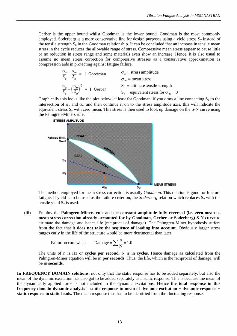
0for stress equivalentS

strength tensileultimateS

stress mean

amplitude stress

me

u

m

a

Gerber is the upper bound whilst Goodman is the lower bound. Goodman is the most commonly

employed. Soderberg is a more conservative line for design purposes using a yield stress Sy instead of

the tensile strength Su in the Goodman relationship. It can be concluded that an increase in tensile mean

stress in the cycle reduces the allowable range of stress. Compressive mean stress appear to cause little

or no reduction in stress range and some materials even show an increase. Hence, it is also usual to

assume no mean stress correction for compressive stresses as a conservative approximation as

compression aids in protecting against fatigue failure.

Graphically this looks like the plot below, at least for Goodman, if you draw a line connecting Su to the

intersection of a and m and then continue it on to the stress amplitude axis, this will indicate the

equivalent stress Se with zero mean. This stress is then used to look up damage on the S-N curve using

the Palmgren-Miners rule.

The method employed for mean stress correction is usually Goodman. This relation is good for fracture

fatigue. If yield is to be used as the failure criterion, the Soderberg relation which replaces Su with the

tensile yield Sy is used.

(iii) Employ the Palmgren-Miners rule and the constant amplitude fully reversed (i.e. zero-mean as

mean stress correction already accounted for by Goodman, Gerber or Soderberg) S-N curve to

estimate the damage and hence life (reciprocal of damage). The Palmgren-Miner hypothesis suffers

from the fact that it does not take the sequence of loading into account. Obviously larger stress

ranges early in the life of the structure would be more detrimental than later.

The units of n is Hz or cycles per second. N is in cycles. Hence damage as calculated from the

Palmgren-Miner equation will be in per seconds. Thus, the life, which is the reciprocal of damage, will

be in seconds.

In FREQUENCY DOMAIN solutions, not only that the static response has to be added separately, but also the

mean of the dynamic excitation has also got to be added separately as a static response. This is because the mean of

the dynamically applied force is not included in the dynamic excitations. Hence the total response in this

frequency domain dynamic analysis = static response to mean of dynamic excitation + dynamic response +

static response to static loads. The mean response thus has to be identified from the fluctuating response.

0.1N

nDamage when occurs Failure


14

The frequency domain random fatigue analysis is summarized as follows: -

(i) Perform equivalent rainflow cycle counting (to generate the PDF) on the response PSD. The

intensity of the signal is given by the RMS. The number of cycles per second is given by the number of

peaks per second, E[P] (peaks/s), function of the moments of the PSD. The total number of cycles, St is

E[P].TSt

Hence the number of cycles for a particular stress range is the probability (from the integral of the

PDF) multiplied by the total number of cycles

tS.dS).S(pcycles of number

Thus, the number of cycles per second for the particular stress range, ni is given by

]P[E.dS).S(p

T/S.dS).S(pn ti

The frequency content or bandedness (in effect the distribution of cycles) of the random PSD needs to

be quantified in order to choose and justify the correct method of generating the PDF. This can be done

by calculating irregularity factor, or by the Dirlik rainflow cycle distribution, both of which is a

function of four moments of the PSD namely m0, m1, m2 and m4.

Performing a frequency domain random analysis on a deterministic (as opposed to narrowband or

broadband random) signal is very conservative. For instance, the PSD of a sine wave with an amplitude

of say 140MPa is simply a spike. We know that the RMS of the sinusoidal time signal is 0.7071 times

the amplitude, hence 100MPa. This RMS will be represented by the area of the PSD. We also know

that generating a random time signal from a PSD will predict a peak amplitude of 3 (to 4.5) times the

RMS, hence 300MPa here. This is because the amplitude distribution of a narrow or broadband signal

is Gaussian. This is much higher than the 140MPa value of the original signal. Thus the frequency

domain approach will be conservative as the greatest damage in a fatigue analysis will be produced by

the large stress ranges even with a relatively low number of cycles.

If we have a narrowband process, all we really need is the RMS to perform a fatigue calculation. The

narrowband solution is traditionally the method employed to ascertain the distribution of the cycles. J.S. Bendat (1964) developed the theoretical basis for the so called Narrow Band solution. However, the fact

that this solution was suitable only for a specific class of response conditions was an unhelpful limitation for

the practical engineer. This was the first frequency domain method for predicting fatigue damage from

PSDs and it assumes that the PDF of peaks is equal to the PDF of stress amplitudes.

The Narrow Band solution was then obtained by substituting the Rayleigh PDF of peaks with the PDF

of stress ranges. The fact that the fatigue PDF is stress range and the Rayleigh PDF is the peak is

accounted for.

The Rayleigh is actually only a function of the RMS and hence just of m0 as RMS = m0. The

narrowband solution is however very conservative (approximately by 100 times) for broadband

processes as it assumes that all positive peaks are matched with corresponding troughs of similar


15

magnitude. The problem with this solution is that by using the Rayleigh PDF, positive troughs and

negative peaks are ignored and all positive peaks are matched with corresponding troughs of similar

magnitude regardless of whether they actually form stress cycles. For wide band response data the method

therefore overestimates the probability of large stress ranges and so any damage calculated will tend to

be conservative. This is illustrated below.

The above figure shows two time histories. The narrow band history is made up by summing two

independent sine waves at relatively close frequencies, while the wide band history uses two sine

waves with relatively widely spaced frequencies. Narrow banded time histories are characterized by the

frequency modulation known as the beat effect. Wide band processes are characterized by the presence

of positive troughs and negative peaks and these are clearly seen in the overhead as a sinusoidal ripple

superimposed on a larger, dominant sine wave. The problem with the narrow band solution is that

positive troughs and negative peaks are ignored and all positive peaks are matched with corresponding

troughs of similar magnitude regardless of whether they actually form stress cycles. To illustrate why

the narrow band solution becomes conservative with wide band histories, take every peak (and trough)

and make a cycle with it by joining it to an imaginary trough (peak) at an equal distance the other side

of the mean level. This is shown in the bottom graph. It is easy to see that the resultant stress signal

contains far more high stress range cycles than were present in the original signal. This is the reason

why the narrow band solution is so conservative.

For broadband signals, Dirlik has produced an empirical closed form expression for the PDF of

rainflow ranges, which was obtained using extensive computer simulations to model the signals using

the Monte Carlo technique. This equation has been found to be a widely applicable solution which

consistently out performs all of the other available methods.


16

Since Bendat first derived the narrow band solution a number of methods have been derived in order to

improve on its short comings. Tunna and Wirsching solutions are both, effectively, corrected versions

of the narrow band approach. Tunna’s equation was developed with specific reference to the railway

industry. Wirsching’s technique was developed with reference to the offshore industry, although it has

been found to be applicable to a wider class of industrial problems. The Chaudhury and Dover, and

Hancock solutions were both developed for the offshore industry. They are both in the form of an

equivalent stress parameter. Neither tend to work well when used for other industrial problems.

Furthermore, the omission of rainflow cycles from the solution output for both approaches is a further

limitation. The Steinberg solution method is used by the electronics industry in the USA.


17

The approach of Steinberg leads to a very simple solution based on the assumption that no stress cycles

occur with ranges greater than 6 rms values. The distribution of stress ranges is then arbitrarily

specified to follow a Gaussian distribution.

Note that the PDF predicts 68.3% time at 2 rms, 27.1% time at 4 rms, and 4.3% time at 6 rms. It is possible

to define the maximum stress range used in the subsequent fatigue analysis. If this is set at 6 rms it is

possible to see that large stress ranges are omitted using this approach. MSC.FATIGUE will set this

value automatically, if not over ridden, to be somewhere around 9 rms for stress range! Anything less

than this is likely to result in an under prediction of fatigue damage. Of course this is counter balanced

by the fact that medium range stress cycles of levels between 4 and 6 rms are over predicted.

Nevertheless it must be stated that this approach is very questionable. It is included only as a means of

allowing designers in the electronics industry, who are used to the Steinberg approach, a means of

comparison.

(ii) Mean (tensile) stress correction cannot be accounted with the PSD method as the PSD contains not

any mean.

(iii) Employ the Palmgren-Miners rule. Failure occurs when

0.1)S(N

nDamage

i

i

Employing the S-N curve,

mi

S

K)S(N

the damage, D is calculated as follows

dS)S(pSK

E[P]

)S(N

nD ,Damage

m

i

i


18

The units of n is Hz or cycles per second. N is in cycles. Hence damage as calculated from the

Palmgren-Miner equation will be in per seconds. Thus, the life, which is the reciprocal of damage, will

be in seconds.

A good method to check whether a PSD has been specified correctly from a time signal is to perform a fatigue

analysis with the PSD as the response PSD in the frequency domain, doing the equivalent rainflow count (with the

Dirlik algorithm) and comparing the stress-life results with a fatigue analysis in the time domain with the time

signal. The rainflow count can also be compared. This checking method will verify that the time signal is random,

Gaussian and stationary. Alternatively, as done usually for any random analysis, the PSD can be converted back

into the time signal and the statistics of the new signal compared with that of the original signal.

An example of a hand-based random frequency domain fatigue analysis is presented. Consider a typical steel S-

N curve.

The idealized response stress PSD is as follows.

The statistics of the PSD are derived.

Two hand methods can be used to approximate the frequency domain random fatigue analysis. One is used when

the PSD is narrowbanded and the other used when the PSD is broadbanded. For a narrowband approximation, an

equivalent solitary sinusoidal wave is derived from the RMS, i.e.


19

Equivalent Sinusoidal Wave Range = 2 x 112 x 2 = 315 MPa.

Hence,

secondper 10x04.3

cycles 2.32292

s/cycles 807.9

315

3728

807.9

S

3728

]P[E

N

nD

4

238.0/1238.0/1

Thus, the life which is the reciprocal is 3293s or 0.92 hours.

For a broadbanded approximation,

Equivalent 1Hz Sinusoidal Wave Range = 2 x 10000 x 2 = 283 MPa.

Equivalent 10Hz Sinusoidal Wave Range = 2 x 2500 x 2 = 141 MPa.

Hence, noting that n corresponds to the frequency of the waves, namely 1Hz and 10Hz,

secondper 10x0314.3

10x0571.110x9743.1

cycles141

3728

Hz 10

cycles283

3728

Hz 1

N

nD

5

55

238.0/1238.0/1

Thus the life is 32987s or 9.2 hours.

The broadbanded approximation is better since the 1Hz and 10Hz is well separated. Note that the foregoing

two hand approximations of the PSD with deterministic signals is not necessarily conservative or

unconservative, but simply approximations. Contrast with the aforementioned fact that representing a

deterministic signal with a PSD and performing a narrowband or broadband solution is conservative, and

also performing a narrowband solution on a broadband PSD is also conservative.

With the rigorous computational method, using the damage expression

dS)S(pSK

E[P].T

)S(N

nD ,Damage

m

i

i

the Narrow Band solution gives life of 0.41 hours (cf. hand based 0.92 hours) and the Dirlik gives life of 2.13 hours

(cf. hand based 9.2 hours).


20

1.1.2.2 Strain-Life (E-N) (Crack Initiation) Uniaxial Fatigue Analysis

Strain life (E-N) prediction is appropriate for low endurance fatigue, i.e. fatigue failures that occur before 104-105

cycles. Low cycles to failure does not necessarily mean a short design life because the frequency of cyclic loading

can be small. For instance, an aircraft fuselage is only pressurized once every flight and so it will take years to

accumulate 104-105 cycles. Failure at low endurance results from stresses and strains that are high and will result in

marked plastic deformation (hysteresis) in every cycle. Hence, strain-life methods are useful when cycles have

some plastic strain component.

The E-N curves are related to the plastic strain range p. This is also the width of the hysteresis loop. The E-N

relationship of the following form applies for most metals up to 105 cycles.

pN = k

A logp versus log N graph plots a straight line. The constant is between 0.5 and 0.6 for most metals at room

temperature.

6 parameters are required to fully define the E-N curve.

With linear finite element analysis, Neuber’s rule can be employed to account for nonlinear stress strain material

curves in the fatigue analysis.

The strain-life fatigue analysis can be performed in the time (not frequency) domain.


21

1.1.2.3 Crack Propagation LEFM Uniaxial Fatigue Analysis

The crack propagation fatigue analysis is more complicated and specialist material should be sought. The crack

propagation fatigue analysis can be performed in the time (not frequency) domain


22

1.1.3 Stress-Life (S-N), Strain-Life (E-N) or Crack Propagation LEFM Multi-axial Fatigue Analysis

Multi-axial fatigue analysis is more complicated and specialist material should be sought.


23

BIBLIOGRAPHY

1. MCEVILY, Arthur, J. Metal Failures, Mechanisms, Analysis, Prevention. John Wiley & Sons, New York,

2002.

2. BISHOP, Dr. Neil. Fundamentals of FEA Based Fatigue Analysis & Vibration Fatigue in MSC.FATIGUE

and MSC.NASTRAN Seminar Notes 2002. MacNeal-Schwendler Corp., England, 2002.

3. MACNEAL-SCHWENDLER CORP. MSC.NASTRAN Fatigue Analysis Quick Start Guide 2001. MacNeal-

Schwendler Corp., Los Angeles, 2001.

4. MACNEAL-SCHWENDLER CORP. MSC.NASTRAN Fatigue Analysis User Guide 2001. MacNeal-

Schwendler Corp., Los Angeles, 2001.

Documents

Vibration Fatigue Analysis in MSC.NASTRAN · PDF fileVibration Fatigue Analysis in MSC.NASTRAN 3 ACKNOWLEDGEMENTS My humble gratitude to the Almighty, to Whom this and all work is