LETTERSPUBLISHED ONLINE: 30 AUGUST 2009 | DOI: 10.1038/NGEO615

Virtual seismometers in the subsurface of theEarth from seismic interferometryAndrew Curtis1,2*, Heather Nicolson1,2,3, David Halliday1,2,4, Jeannot Trampert5 and Brian Baptie2,3

The Earth’s interior can be imaged by analysing the recordsof propagating seismic waves. However, the global arrayof permanent seismometers that record seismic energy isconfined almost exclusively to land-based sites. This limitsthe resolution of subsurface images, and results in relativelyfew local measurements from areas of great geologicaland tectonic interest (for example, the mid-ocean ridgesand the Tibetan plateau)1. Here we use an unconventionalform of seismic interferometry2–5 to turn earthquakes intovirtual seismometers located beneath the Earth’s surface.Seismic waves generated by one earthquake lead to transientstrain in the subsurface at other locations around theglobe. This strain can be quantified from seismograms ofindependent earthquakes that have occurred in those locations.This technique can therefore provide information on thesubsurface strain in regions of the globe that lack instrumentalnetworks. Applying our method to earthquakes in Alaskaand the southwestern United States, we show that theinformation that can be obtained from these earthquakesabout other such events is consistent with that provided byinstrumental seismometers. Our approach may allow real-time, non-invasive, subsurface seismic strain monitoring,particularly in areas remote from instrumental networks.

To interrogate the Earth’s subsurface at depths greater than afew kilometres, traditional seismology analyses seismic wave energyfrom earthquakes. Other energy recorded in seismograms, such asambient Earth oscillation, is considered noise and is excluded fromanalysis. Since 2003, however, methods of seismic interferometryhave been developed to synthesize impulsive source seismogramsfrom ambient noise recorded at two seismic receivers2. Theseseismograms simulate the situation where energy from a relativelyimpulsive, imagined or ‘virtual’ source occurring at the location ofone receiver was recorded by the other.

In Fig. 1a we show a sketch of source–receiver geometriesused for interferometry. Recordings of each boundary sourceat the pair of receivers are cross-correlated, then integrated(summed) over all sources. The result gives the seismogramthat would have been recorded at one receiver if the otherreceiver had instead been a source. Theoretically such seismogramscan be constructed provided the sources of seismic energy aredistributed to form an enclosing boundary of sources, althoughthe latter geometrical constraint can often be relaxed in practice(see below). Given a suitable receiver geometry, interferometryobviates the need for actual earthquake sources for imaging theEarth2,6–10. Variations of interferometric theory work in attenuativemedia, for diffusive, electromagnetic and electro-kinetic energypropagation11–14, when using active rather than passive sources of

1School of GeoSciences, University of Edinburgh, Grant Institute, West Mains Road, Edinburgh EH9 3JW, UK, 2ECOSSE (Edinburgh Collaborative ofSubsurface Science and Engineering), UK, 3British Geological Survey, Murchison House, Kings Buildings, West Mains Road, Edinburgh EH9 3LA, UK,4Schlumberger Cambridge Research, High Cross, Madingley Road, Cambridge, CB3 0EL, UK, 5Faculteit Aardwetenschappen, University of Utrecht,Postbus 80.021, Utrecht, Netherlands. *e-mail: Andrew.Curtis@ed.ac.uk.

elastic or electromagnetic energy15–21 and can be used to create novelmethods for wavefield simulation22–24.

Although in principle interferometry frees seismologists fromconstraints imposed by the global distribution of earthquakes,which is strongly biased towards active margins and mid-oceanridges, the global receiver distribution is also strongly biased(Supplementary Fig. S2). More than two-thirds of the Earth’ssurface is covered by liquid water or ice, rendering receiverinstallation difficult and expensive. Even many land-based areashave few receivers because they are geographically or politicallyinhospitable (for example, the Tibetan and Andean plateaus,Central Africa). Hence, most of the Earth’s subsurface can onlybe interrogated using long earthquake–receiver or receiver–receiverpaths of energy propagation. This provides relatively poor spatialresolution of some of the most intriguing tectonic, geologicaland geophysical phenomena such as mid-ocean ridges and plateconvergence zones, and consequently there is a need for data to berecorded locally to such phenomena.

By taking the reciprocal of its usual form, in the SupplementaryMethods we show that the impulsive source form of interferometrycan also be used in the opposite sense: to turn any energy sourceinto a virtual sensor. In this form, we apply interferometry usingsources enclosed within a boundary of receivers (Fig. 1b). Thisapproach is related to that of ref. 25, but they used the passivenoise (rather than impulsive source) form of interferometry. Wedemonstrate a substantial improvement over their results. It has

x2

x’ x’ x’

x2 x2

x1 x1 x1V V V

S S S

a cb

Figure 1 | Schematic overview of seismic interferometric methods.a, So far, seismic interferometry estimates the Green’s function betweenthe locations of two receivers (triangles) at x1 and x2, by cross-correlatingrecorded waves radiating from energy sources (stars), on some boundary Ssurrounding volume V. b, In the Supplementary Information we usereciprocity to approximate the same Green’s function given energy sourcesat x1 and x2 recorded at receivers on S. c, It has been shown that for a and b,the Green’s function can be approximated using only receivers around theextension of the x1−x2 line (within the grey areas)28.

NATURE GEOSCIENCE | ADVANCE ONLINE PUBLICATION | www.nature.com/naturegeoscience 1© 2009 Macmillan Publishers Limited. All rights reserved.

LETTERS NATURE GEOSCIENCE DOI: 10.1038/NGEO615

0 1,000 2,000 3,000 4,000 5,000 6,000 7,000¬1

0

1

Delay time (s)

0 1,000 2,000 3,000 4,000 5,000 6,000 7,000Delay time (s)

0 1,000 2,000 3,000 4,000 5,000 6,000 7,000Delay time (s)

0 1,000 2,000 3,000 4,000 5,000 6,000 7,000Delay time (s)

Nor

mal

ized

am

plitu

deN

orm

aliz

ed a

mpl

itude

Nor

mal

ized

am

plitu

deN

orm

aliz

ed a

mpl

itude

Latit

ude

(N)

Longitude (E)

¬1

0

1

¬1

0

1

¬1

0

1

a

b

c

d

e

75°

5°10°15°

20°25°30°35°

40°

45°

50°

55°

60°

65°

70°

90° 100° 110° 120° 130° 140° 150° 160° 170° 180° 190° 200° 210° 220° 230° 240° 250°

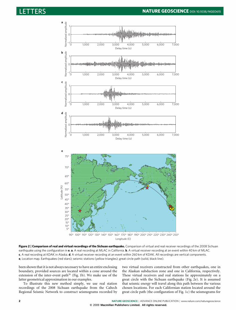
Figure 2 | Comparison of real and virtual recordings of the Sichuan earthquake. Comparison of virtual and real receiver recordings of the 2008 Sichuanearthquake using the configuration in e. a, A real recording at MLAC in California. b, A virtual receiver recording at an event within 40 km of MLAC.c, A real recording at KDAK in Alaska. d, A virtual receiver recording at an event within 260 km of KDAK. All recordings are vertical components.e, Location map. Earthquakes (red stars); seismic stations (yellow triangles); great circle path (solid, black line).

been shown that it is not always necessary to have an entire enclosingboundary, provided sources are located within a cone around theextension of the inter-event path26 (Fig. 1b). We make use of thelatter geometrical approximation in our examples.

To illustrate this new method simply, we use real stationrecordings of the 2008 Sichuan earthquake from the CaltechRegional Seismic Network to construct seismograms recorded by

two virtual receivers constructed from other earthquakes, one inthe Alaskan subduction zone and one in California, respectively.These virtual receivers and real stations lie approximately on agreat circle with the Sichuan earthquake (Fig. 2e). It is assumedthat seismic energy will travel along this path between the variouschosen locations. For each Californian station located around thegreat circle path (the configuration of Fig. 1c) the seismograms for

2 NATURE GEOSCIENCE | ADVANCE ONLINE PUBLICATION | www.nature.com/naturegeoscience

© 2009 Macmillan Publishers Limited. All rights reserved.

NATURE GEOSCIENCE DOI: 10.1038/NGEO615 LETTERSWestern USA station map

236° 248°32°

34°

36°

38°

40°

42°

238° 240° 242° 244° 246°

R06C

MLAC

4

3

2

1

Latit

ude

(N)

Longitude (E)

Figure 3 | South-west USA location map. Earthquakes (red stars)numbered 1–4; seismic stations used in interferometry (blue triangles);seismic stations for comparison (yellow triangles); focal mechanisms ofvirtual receivers are shown as standard lower hemisphere projections nearto their locations. Dashed lines indicate inter-earthquake paths; solid linesconnected by arcs indicate the region within which receivers were locatedfor each earthquake pair.

the Sichuan and virtual receiver earthquakes are cross-correlated,then the resulting cross-correlations are summed. In Fig. 2 we showthe real recordings of the Sichuan earthquake at stations locatedclose to each virtual receiver (Fig. 2a and c) and the resulting virtualreceiver records (Fig. 2b and d).

The real and virtual traces should not be exactly the samebecause the virtual receiver records strain whereas real receiversmeasure displacement (Supplementary Methods). In addition, thestations used for comparison are not collocated with the virtualreceivers. Nevertheless, the similarity between the real and virtualreceiver recordings is clear.

As the match in Fig. 2 is not perfect, we consider test casesusing earthquake and receiver geometries that allow a deeperanalysis of the method. The Supplementary Methods shows thatvirtual sensors inherit the spatio-temporal response function of theoriginal earthquake source: those constructed from purely normaland purely thrust earthquakes thus measure strains in a vertical–horizontal plane, whereas those from strike–slip earthquakesmeasure strain in the purely horizontal plane. Those constructedfrom subsurface explosions or implosions measure volumetricexpansion of the rock mass (the solid-body equivalent of a pressuresensor in a fluid)27. Supplementary Table S1 summarizes the straincomponents measured for each canonical earthquake or explosivesource mechanism.

Figure 3 shows earthquakes and stations used for verification.Two earthquakes with approximately canonical (strike–slip andnormal) moment tensor sources were chosen to be converted intovirtual sensors because (1) seismometers (MLAC andR06C) exist intheir local vicinity for comparison, (2) they had a well-constrainedmoment tensor source mechanism, (3) they had the lowest possiblemagnitude subject to constraints (1) and (2) and hence are spatially

0 50 100 150 200 250 300 350 400Delay time (s)

Delay time (s)

0 50 100 150 200 250 300 350 400

Nor

mal

ized

am

plitu

de

0

0.2

0.4

0.6

0.8

1.0

Am

plitu

de

¬1.0

¬0.5

0

0.5

1.0

Figure 4 | Comparison of real and virtual recordings in California.Comparison of seismograms (top) and envelope functions (bottom) forearthquake 1 recorded by the normal virtual receiver 4 (solid line) with thedirectly recorded, inverted, time derivative of the radial componentmeasurements from seismometer R06C (dashed line). Virtual receiverrecords are constructed using 15 stations from the USArray and Berkeleyseismic networks (Fig. 3), and all records are band-passed between 15 and33 seconds period.

and temporally as localized as possible, reducing associated relativephase differences between recordings on seismometers and virtualsensors (the source times used for the seismometer recordings arethose from the International Seismology Centre (ISC) catalogue;no centroid moment tensor (CMT) source mechanisms andtimings were available).

We analysed seismograms from two other earthquakes recordedon these virtual sensors, one chosen to have the source–virtualsensor path aligned roughly east–west, the other chosen to have aroughly perpendicular path. We compare strain recordings of theseevents on the virtual sensors with estimates of strain constructedfrom recordings of particle velocity from the neighbouringseismometers (see theMethods section below).

Virtual sensors were constructed by integrating (summing)unweighted recordings from a subset of other available seismome-ters that did not include either comparison seismometer (Sup-plementary Methods, Equation (S18)). Each subset consisted ofseismometers within a cone around the propagation path directionat the virtual sensor (Fig. 3), as these are expected to record themainenergy that integrates constructively within the virtual receiverseismogram28. Conclusions herein are robust to changes in thesubtending angle of the cone.

Figure 4 shows earthquake 1 recorded by the virtual sensorconstructed from the N–S oriented normal fault. This virtualreceivermeasures the difference between the e33 and e11 componentsof the strain. Although we do not have a comparison measurementfor the e33 component (see Supplementary Fig. S4, which showsa comparison to the vertical component of particle velocity), wecan construct a comparison seismogram for the e11 component(see Methods). Figure 4 shows that the fit is excellent. Hence, forthis event at this station, the signal is probably dominated by thehorizontal strain component e11. As the vertical strain componentis approximately related to the derivative of the Rayleigh waveeigenfunctions with depth beneath the virtual receiver, we infer thatthe eigenfunction is likely to be approximately constant with depthat the earthquake location.

A strike–slip virtual receiver such as earthquake 3 in Fig. 3records the sum of the e12 and e21 components of the strain (Supple-mentary Methods, Equations (S30)–(S33)). In the Supplementary

NATURE GEOSCIENCE | ADVANCE ONLINE PUBLICATION | www.nature.com/naturegeoscience 3© 2009 Macmillan Publishers Limited. All rights reserved.

LETTERS NATURE GEOSCIENCE DOI: 10.1038/NGEO615

Discussion, Supplementary Fig. S2 shows that the virtual and realrecordings of earthquake 1 using this strike–slip virtual receiveralso compare well. Supplementary Fig. S5 shows the case whenearthquake 2 is recorded on a virtual receiver constructed fromearthquake 4. In this geometry the Supplementary Methods showsthat the virtual sensor records only the e33 component, providing afundamentally newmeasurement in seismology.

Previously, Hong andMenke25 estimated virtual seismograms bya different method. They added active source recordings together togenerate pseudo-noise sequences and then applied the passive noiseform of interferometry to estimate inter-source responses (thatis, they sum over receivers, then cross-correlate). Unfortunately,accurate seismogram construction from passive noise requiresmuch longer time series than are afforded by typical earthquakeseismograms23, and consequently in Supplementary Fig. S5 weshow that their method produces less accurate seismogramapproximations. Our approach is different: we use the impulsivesource form of interferometry by first cross-correlating responsesand only then summing over receivers. This requires only the actual,recorded seismograms at each receiver.

Although we formulated theory only for acoustic and elasticwave propagation (see Supplementary Methods), this can be ex-tended into forms appropriate for diffusive, attenuating, electro-magnetic or electro-kinetic energy propagation11–14. It is appliedhere to earthquake sources, but we could equally construct virtualsensors from fractures occurring in stressed solid material in alaboratory, or from impulsive pressure sources in liquid or gas, pro-vided energy from such sources is recorded using an appropriatelyplaced array of receivers.

The inter-earthquake seismogram is obtained by back-projecting data recorded from one earthquake through empiricallyrecorded Green’s functions from another, an explicit elasticexpression of the acoustic time-reversal experiment of Derodeand colleagues29. However, the method also converts the datafrom particle displacement (or time derivatives thereof) at thereal seismometers to strain due to seismic waves at the subsurfacelocations, the strain components matching those of the originalsource. Also, as this method essentially back-projects recordingsto the virtual sensor location, it is equally possible to back-projectother signals such as passive noise recordings to either or both ofthe pair of subsurface source locations. This offers the possibilityof monitoring inter-earthquake Green’s functions as a function oftime either before or after the original earthquakes occurred, byusing standard passive noise interferometry2–5.

In the exploration industry, seismic-frequency strain recordingshave been shown to be particularly useful for wavefield analysis andsubsurface imaging26,27. The direct, non-invasive sensitivity to strainprovided by the virtual seismometers introduced here is the firstsuchmeasurement within the interior of a solid. This holds promisefor analysing stress or strain triggering of earthquakes by passingseismic waves, for example, as no other method has the potential toprovide such deep or such widely distributed measurements of thestrain field in the Earth’s subsurface.

MethodsIn the Supplementary Methods we present a general acoustic and elasticformulation for constructing virtual sensors using interferometry. We also developtheory for the particular case of an earthquake double-couple moment tensorsource radiating Rayleigh and Love surface waves, as so far, seismic interferometryhas derived useful information largely from the reconstruction of surface waves.We thus derive precisely which components of surface wave strain are recordedby virtual receivers constructed from canonical normal, thrust and strike–slipearthquakes, allowing verification of the method by comparison with directlyrecorded seismograms in these cases (Supplementary Table S1).

A potential problem in verifying virtual receiver seismograms (for example,in Fig. 4) is that no direct seismic frequency strain sensors exist in the Earthclose to earthquakes for comparison. To make direct comparisons possible, inprinciple one could construct horizontal strain measurements by computing

scaled differences between closely spaced seismometers27, but in the frequencyrange considered here (15–33 s period) across the southwestern US this is generallynot possible because the seismometer distribution is spatially aliased. Insteadwe derive estimates of the scaled horizontal strain in a direction in line with thesource–seismometer path by taking time derivatives of measured seismograms.This results in frequency domain multiplication by iω= ick, where ω and k aretemporal and in-line spatial frequencies, respectively, and c is the phase velocity.Thus we approximate a spatial derivative (multiplication by ik) assuming thatthe unknown phase velocity c does not change rapidly within the frequency bandconsidered (we also took account of the azimuth of propagation, which can changethe sign of the horizontal strain estimates).

There is no equivalent operation for approximating vertical strains in theexamples presented above. Vertical strain measurements from virtual receiverstherefore constitute new information about Earth vibrations.

If an earthquake is considered to be temporally impulsive with moment tensorM1 and is recorded by a virtual sensor constructed from another earthquake withmoment tensorM2, the data consist of a sum of strain Green’s functions betweenthe locations of the two earthquakes, scaled by the product of the respectivemomenttensor components (Supplementary Methods, Equations (S15)–(S18)). However,earthquake sources are also generally non-impulsive. If Wi(ω) is the frequencydomain representation of the source time function of earthquake i, the seismogramsrecorded at the virtual sensor are modulated byW2W1

∗ (Supplementary Methods,Equations (S10) and (S11)). Hence, if for example the two source time functionswere similar,W2 ≈W1, the recorded data would consist of inter-earthquake strainGreen’s functions modulated by the autocorrelation of the source time function,shifted in time by t2− t1, where ti is the origin time of earthquake i. We remove thattime shift in the results presented in this letter and in Supplementary Methods. Asa consequence, compared with zero-phase seismometer recordings, residual phaseshifts in the virtual sensor records are caused by differences between the two sourcetime functionsW1 andW2.

Received 14 April 2009; accepted 28 July 2009; published online30 August 2009

References1. Bijwaard, H. & Spakman, W. Non-linear global P-wave tomography by iterated

linearized inversion. Geophys. J. Int. 141, 71–82 (2000).2. Campillo, M. & Paul, A. Long-range correlations in the diffuse seismic coda.

Science 299, 547–549 (2003).3. Shapiro, N. & Campillo, M. Emergence of broadband Rayleigh waves from

correlations of the ambient seismic noise.Geophys. Res. Lett. 31, L07614 (2004).4. Shapiro, N., Campillo, M., Stehly, L. & Ritzwoller, M. High-resolution

surface-wave tomography from ambient seismic noise. Science 307,1615–1617 (2005).

5. Gertstoft, P., Sabra, K. G., Roux, P., Kuperman, W. A. & Fehler, M. C.Green’s functions extraction and surface-wave tomography from microseismsin southern California. Geophysics 71, SI23–SI31 (2006).

6. Claerbout, J. F. Synthesis of a layered medium from its acoustic transmissionresponse. Geophysics 33, 264–269 (1968).

7. Wapenaar, K. Synthesis of an inhomogeneous medium from its acoustictransmission response. Geophysics 68, 1756–1759 (2003).

8. Wapenaar, K. & Fokkema, J. Reciprocity theorems for diffusion, flow, andwaves. J. Appl. Mech. 71, 145–150 (2004).

9. Wapenaar, K., Thorbecke, J. & Draganov, D. Relations between reflectionand transmission responses of three-dimensional inhomogeneous media.Geophys. J. Int. 156, 179–194 (2004).

10. Wapenaar, K. & Fokkema, J. Green’s function representations for seismicinterferometry. Geophysics 71, SI33–SI44 (2006).

11. Slob, E., Draganov, D. &Wapenaar, K. Interferometric electromagnetic Green’sfunctions representations using propagation invariants. Geophys. J. Int. 169,60–80 (2007).

12. Slob, E. & Wapenaar, K. Electromagnetic Green’s functions retrieval bycross-correlation and cross-convolution inmedia with losses.Geophys. Res. Lett.34, L05307 (2007).

13. Snieder, R. Extracting the Green’s function of attenuating heterogeneous mediafrom uncorrelated waves. J. Acoust. Soc. Am. 121, 2637–2643 (2007).

14. Snieder, R., Wapenaar, K. & Wegler, U. Unified Green’s function retrievalby cross-correlation; connection with energy principles. Phys. Rev. E 75,036103 (2007).

15. Bakulin, A. & Calvert, R. in 74th Annual International Meeting, SEG,Expanded Abstracts 2477–2480 (SEG, 2004).

16. Bakulin, A. & Calvert, R. The virtual source method: Theory and case study.Geophysics 71, SI139–SI150 (2006).

17. Dong, S., He, R. & Schuster, G. in 76th Annual International Meeting, SEG,Expanded Abstracts 2783–2786 (SEG, 2006).

18. Snieder, R., Wapenaar, K. & Larner, K. Spurious multiples in seismicinterferometry of primaries. Geophysics 71, SI111–SI124 (2006).

19. Halliday, D. F., Curtis, A., van Manen, D.-J. & Robertsson, J. Interferometricsurface wave isolation and removal. Geophysics 72, A69–A73 (2007).

4 NATURE GEOSCIENCE | ADVANCE ONLINE PUBLICATION | www.nature.com/naturegeoscience

© 2009 Macmillan Publishers Limited. All rights reserved.

NATURE GEOSCIENCE DOI: 10.1038/NGEO615 LETTERS20. Mehta, K., Bakulin, A., Sheiman, J., Calvert, R. & Snieder, R. Improving the

virtual source method by wavefield separation.Geophysics 72,V79–V86 (2007).21. Halliday, D. F., Curtis, A. & Kragh, E. Seismic surface waves in a suburban

environment—active and passive interferometric methods. The Leading Edge27, 210–218 (2008).

22. van Manen, D.-J., Robertsson, J. O. A. & Curtis, A. Modeling ofwave propagation in inhomogeneous media. Phys. Rev. Lett. 94,164301–164304 (2005).

23. van Manen, D.-J., Curtis, A. & Robertsson, J. O. A. Interferometric modelingof wave propagation in inhomogeneous elastic media using time reversal andreciprocity. Geophysics 71, SI47–SI60 (2006).

24. van Manen, D.-J., Robertsson, J. O. A. & Curtis, A. Exact wavefield simulationfor finite-volume scattering problems. J. Acoustic. Soc. Am. Express Lett. 122,EL115–EL121 (2007).

25. Hong, T.-K. & Menke, W. Tomographic investigation of the wear alongthe San Jacinto fault, southern California. Phys. Earth Planet. Inter. 155,236–248 (2006).

26. Robertsson, J. O. A. & Curtis, A. Wavefield separation using densely deployed,three component, single sensor groups in land surface seismic recordings.Geophysics 67, 1624–1633 (2002).

27. Curtis, A. & Robertsson, J. Volumetric wavefield recording and near-receivergroup velocity estimation for land seismics. Geophysics 67, 1602–1611 (2002).

28. Snieder, R. Extracting the Green’s function from the correlation of coda waves:A derivation based on stationary phase. Phys. Rev. E 69, 046610 (2004).

29. Derode, A. et al. Recovering the Green’s function from field–field correlationsin an open scattering medium. J. Acoust. Soc. Am. 113, 2973–2976 (2003).

AcknowledgementsThe earthquake data used in this study were obtained from the IRIS DataManagement Centre.

Author contributionsA.C. and D.H. developed the theory, H.N. created the examples and J.T. andB.B. contributed ideas that helped to shape the manuscript.

Additional informationSupplementary information accompanies this paper on www.nature.com/naturegeoscience.Reprints and permissions information is available online at http://npg.nature.com/reprintsandpermissions. Correspondence and requests for materials should beaddressed to A.C.

NATURE GEOSCIENCE | ADVANCE ONLINE PUBLICATION | www.nature.com/naturegeoscience 5© 2009 Macmillan Publishers Limited. All rights reserved.