VISCOTHERMAL WAVE PROPAGATION INCLUDING ACOUSTO …bctill/papers/numacoust/Beltman_19… · · 2009-07-13In tribology, the Reynolds ... the dimensions and the wavelength have to

Journal of Sound and <ibration (1999) 227(3), 555}586Article No. jsvi.1999.2355, available online at http://www.idealibrary.com on

VISCOTHERMAL WAVE PROPAGATION INCLUDINGACOUSTO-ELASTIC INTERACTION, PART I: THEORY

W. M. BELTMAN

Department of Mechanical Engineering, ;niversity of ¹wente, P.O. Box 217,7500 AE Enschede, ¹he Netherlands

(Received 15 December 1998, and in ,nal form 6 May 1999)

This research deals with pressure waves in a gas trapped in thin layers or narrowtubes. In these cases viscous and thermal e!ects can have a signi"cant e!ect on thepropagation of waves. This so-called viscothermal wave propagation is governedby a number of dimensionless parameters. The two most important parametersare the shear wave number and the reduced frequency. These parameters were usedto put into perspective the models that were presented in the literature. Theanalysis shows that the complete parameter range is covered by three classes ofmodels: the standard wave equation model, the low reduced frequency model andthe full linearized Navier}Stokes model. For the majority of practical situations,the low reduced frequency model is su$cient and the most e$cient to describeviscothermal wave propagation. The full linearized Navier}Stokes model shouldonly be used under extreme conditions.

( 1999 Academic Press

1. INTRODUCTION

The propagation of sound waves with viscothermal e!ects has been investigated inseveral scienti"c disciplines. The propagation of sound waves in tubes wasinvestigated already by Kirchho! and Rayleigh [1]. In tribology, the Reynoldsequation is used to calculate the pressure distribution in #uid "lms trapped betweenmoving surfaces. Reynolds' theory assumes that the inertial e!ects are negligible: itis based on a so-called creeping #ow assumption. Increasing machine speeds andthe use of gas bearings initiated research on the role of inertia [2}10]. In -uidmechanics, the propagation of sound waves in tubes and in particular the steadystreaming phenomenon have been extensively discussed [11}14]. Two early paperson thin "lm theory in acoustics were presented by Maidanik [15] and Ungar andCarbonell [16]. A large number of investigations have been carried out since then.Consequently, a seemingly endless variety of models is available now to deal withviscothermal e!ects in acoustic wave propagation.

The variety of models is deceiving. The models that were presented in acousticscan be grouped into three basic categories. Key words in the characterization ofthese models are: pressure gradient across layer thickness or tube cross-section, andthe incorporation of e!ects such as compressibility and thermal conductivity.

0022-460X/99/430555#32 $30.00/0 ( 1999 Academic Press

556 W. M. BELTMAN

The most extensive type of model clearly must be based on a solution of the fullset of basic equations. This means that, for instance, all the terms in the linearizedNavier}Stokes equations are taken into account. The second type of modelincorporates a pressure gradient. However, not all the terms in the basic equationsare retained. In some models, for instance, thermal e!ects are neglected. Thesimplest model, the low reduced frequency model, assumes a constant pressureacross the layer thickness or tube cross-section. The e!ects of inertia, viscosity,compressibility and thermal conductivity are accounted for. This leads to a verystraightforward and useful model.

The main aim of this paper is to provide a framework for putting modelsfor viscothermal wave propagation into perspective. It is not the intentionof the author to present a list of all papers related to viscothermal wavepropagation. Wave propagation is considered from a standard acoustical pointof view. Non-linear e!ects are therefore neglected. For an extensive overviewof non-linear e!ects and viscothermal wave propagation the reader is referredto the papers by Makarov and Ochmann [17}19] and Too and Lee [20]. Makarovand Ochmann present an overview of the literature, based on more than 300references.

The present analysis is based on the use of dimensionless parameters. It is anextension of the work on the propagation of sound waves in cylindrical tubes, aspresented by Tijdeman [21]. The three groups of models are all written ina dimensionless form. As a consequence, a number of dimensionless parametersappear in the equations. With the help of these parameters the range of validity foreach group is indicated. Furthermore, for each type of model a short list of relatedliterature is given. The list o!ers information about parameter ranges andapplications. Based on this information, one can easily determine which modelshould be used for a given application. Finally, the problem of acoustic-elasticcoupling, i.e., the mutual interaction between vibrating #exible surfaces and thinlayers of gas or #uid, is addressed for each type of model.

2. BASIC EQUATIONS

2.1. DERIVATION OF EQUATIONS

The basic equations governing the propagation of sound waves are the linearizedNavier}Stokes equations, the equation of continuity, the equation of state for anideal gas and the energy equation. In the absence of mean #ow the equations can bewritten as

o0Lv6 /Lt"!$1 p6 #A

43

k#gB $1 ($1 ) v6 )!k$1 ]($1 ]v6 )

o0($1 ) v6 )#LoN /Lt"0, p6 "o6 R

0¹M ,

o0C

pL¹M /Lt"jDM ¹M #LpN /Lt, (1)

VISCOTHERMAL WAVE PROPAGATION 557

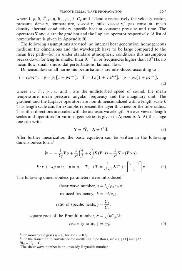
where v6 , p, o6 , ¹M , k, g, R0, o

0, j, C

pand t denote respectively the velocity vector,

pressure, density, temperature, viscosity, bulk viscosity,s gas constant, meandensity, thermal conductivity, speci"c heat at constant pressure and time. Theoperators $1 and DM are the gradient and the Laplace operator respectively. (A list ofnomenclature is given in Appendix B).

The following assumptions are used: no internal heat generation; homogeneousmedium: the dimensions and the wavelength have to be large compared to themean free path*for air under standard atmospheric conditions this assumptionbreaks down for lengths smaller than 10~7 m or frequencies higher than 109 Hz; nomean #ow; small, sinusoidal perturbations; laminar #ow.t

Dimensionless small harmonic perturbations are introduced according to

v6 "c0ve*ut, pN "p

0[1#pe*ut], ¹M "¹

0[1#¹e*ut], o6 "o

0[1#oe*ut],

(2)

where c0, ¹

0, p

0, u and i are the undisturbed speed of sound, the mean

temperature, mean pressure, angular frequency and the imaginary unit. Thegradient and the Laplace operators are non-dimensionalized with a length scale l.This length scale can, for example, represent the layer thickness or the tube radius.The other directions are scaled with the acoustic wavelength. An overview of lengthscales and operators for various geometries is given in Appendix A. At this stageone can write

$"l$1 , D"l2DM . (3)

After further linearization the basic equation can be written in the followingdimensionless form:A

iv"!

1kc

$p#1s2 A

43#nB $ ($ ) v)!

1s2

$]($]v),

$ ) v#i ko"0, p"o#¹, i¹"

1s2p2

D¹#iCc!1

c D p. (4)

The following dimensionless parameters were introduced:}

shear wave number, s"lJo0u/k ;

reduced frequency, k"ul/c0;

ratio of speci"c heats, c"C

pC

v

;

square root of the Prandtl number, p"JkCp/j ;

viscosity ratio, m"g/k . (5)

sFor monatomic gases g"0, for air g"0)6ktFor the transition to turbulence for oscillating pipe #ows, see e.g. [14] and [72].AR

0"C

p!C

v}The shear wave number is an unsteady Reynolds number

558 W. M. BELTMAN

Here, Cv

is the speci"c heat at constant volume. The dimensionless equationsindicate that the viscothermal wave propagation is governed by a number ofdimensionless parameters. These parameters can be used to characterize di!erent#ow regimes. Furthermore, they enable solutions given in the literature to be putinto perspective: assumptions or restrictions of models can be quanti"ed in terms ofthese parameters.

The parameters c and p depend solely on the material properties of the gas. Themost important parameters are the shear wave number and the reduced frequency.The shear wave number is a measure for the ratio between the inertial e!ects andthe viscous e!ects in the gas: it is an unsteady Reynolds number. For large shearwave numbers the inertial e!ects dominate, whereas for low shear wave numbersthe viscous e!ects are dominant. In physical terms the shear wave numberrepresents the ratio between the length scale, e.g. the layer thickness or tube radius,and the boundary layer thickness. The reduced frequency represents the ratiobetween the length scale and the acoustic wavelength. For very low values of thereduced frequency, the acoustic wavelength is very large compared to the lengthscale l. The parameters presented in this section are essential for the choice of anappropriate model for a speci"c situation.

2.2. BOUNDARY CONDITIONS

In order to solve the set of equations boundary conditions must be imposed. Thequantities of interest here are the (dimensionless amplitudes of the) velocity,temperature, pressure and density. Boundary conditions for the density are usuallynot imposed, and will therefore not be considered here.

2.2.1. <elocity

At a gas}wall interface, a continuity of velocity is assumed in most cases.Continuity of velocity usually implies that the tangential velocity is zero: a no-slipcondition is imposed. The normal velocity is equal to the velocity of the wall. In thisway, the acousto-elastic coupling between vibrating structures and viscothermalgases is established. For rare"ed gases, investigations indicate that it is moreappropriate to use a jump in velocity with corresponding momentumaccommodation coe$cientss [22, 23]. For gases under atmospheric conditionsa simple continuity of velocity condition su$ces.

2.2.2. ¹emperature

The most common boundary conditions are isothermal walls or adiabatic walls.For an isothermal wall the temperature perturbation is zero, whereas for anadiabatic wall the gradient of the temperature normal to the wall vanishes. When

sIn this case one assumes a jump condition at the interface, e.g. a velocity slip or temperature jump.For the temperature the boundary equation then becomes: ¹!¹

w"!¸$¹ ) n, where ¹

wis the wall

temperature, ¸ is related to the thermal accommodation coe$cients and n is the outward normal.


the product of the speci"c heat per unit volume and the thermal conductivity of thewall material substantially exceeds the corresponding product for the gas, theassumption of isothermal walls is usually accurate (see, e.g. reference [24]).

Again, for rare"ed gases, it is more appropriate to use a jump condition [22, 23].This condition allows for a jump in temperature across the gas}wall interface witha thermal accommodation coe$cient. In the literature, some models werepresented to model walls with "nite heat conduction properties (see, Reference[25]).

A very interesting consequence of thermal e!ects is the phenomenon of thermallydriven vibrations. As a boundary condition, one could for instance imposea varying temperature across the length of a tube. This temperature gradient drivespressure pulsations in the gas. This e!ect will not be addressed here: for detaileddiscussion the reader is referred to the literature [26}33].

2.2.3. Pressure

At the ends of a tube or layer boundary conditions can be imposed for thepressure, for instance a pressure release. In the present investigation end e!ects areneglected. For a more detailed discussion on this subject the reader is referred to theliterature [34}39].

2.3. GEOMETRIES AND CO-ORDINATE SYSTEMS

The basic equations were given in terms of gradient and Laplace operators. InAppendix A an overview of length scales, dimensionless co-ordinates, gradientoperators and Laplace operators is given for a number of geometries.

3. FULL LINEARIZED NAVIER}STOKES MODEL


The most extensive type of model is that obtained by solving the complete set ofbasic equations. The derivation in this section is based on the paper by Bruneauet al. [40]. Their formulation however was rewritten in terms of dimensionlessquantities for the present study. In order to solve this problem, the velocity iswritten as the sum of a rotational velocity v

v, due to viscous e!ects, and a solenoidal

velocity vl

v"vv#v

l, (6)

where these satisfy

$ ) vv"0, $]v

l"0. (7)

The following relationship was used in this derivation:

$]($]vv),$ ($ ) v

v)!($ )$)v

v"!Dv

v. (8)

560 W. M. BELTMAN

Inserting these expressions into the basic equations and taking the rotation anddivergence gives the following set of dimensionless equations:

ivl!

1s2 A

43#nBD v

l"!

1kc

$p,

$ ) vl#iko"0, iv

v!

1s2

Dvv"0, p"o#¹, i¹"

1s2p2

D¹#iCc!1

c D p.

(9)

After some algebraic manipulations the following equation can be derived in termsof the temperature perturbation:

is2p2 C1#

ick2

s2 A43#nBD DD¹#C1#

ik2

s2 A43#nB#

cp2DDD¹#k2¹"0. (10)

It can easily be veri"ed that both vland p also satisfy this equation. Note that if

m"0 in this equation, i.e., the bulk viscosity is neglected, a dimensionless equationis obtained that was already derived by Kirchho! and Rayleigh [1].

3.2. SOLUTION STRATEGY

The equation for the temperature perturbation can be written in a factorizedform,

[D#k2a] [D#k2

h] ¹"0, (11)

where kaand k

hare the acoustic and entropic wave numbers respectively,

k2a"

2k2

C1#JC2

1!4C

2

, k2h"

2k2

C1!JC2

1!4C

2

, (12)

in which:

C1"C1#

ik2

s2 CA43#mB#

cp2DD , C

2"

ik2

s2p2 C1#ick2

s2 A43#mBD . (13)

The solution for the temperature perturbation can be written as

¹"Aa¹

a#A

h¹

h, (14)

where ¹aand ¹

hare referred to as the acoustic and the entropic temperatures. The

constants Aaand A

hremain to be determined from the boundary conditions. The

quantities ¹a

and ¹h

are the solutions of

[D#k2a]¹

a"0, [D#k2

h]¹

h"0. (15)

Once the solution for the temperature is known, the values for the velocity vland

the pressure p can be expressed in terms of Aa, A

h, ¹

aand ¹

a. One obtains

p"Cc

c!1D CAa C1!ik2

as2

1p2D¹a

#Ah C1!

ik2h

s21p2D¹hD ,


vl"v

la#v

lh"a

aA

a$¹

a#a

hA

h$¹

h,

aa"

ikc C

cc!1D C

1!ik2

as2

1p2

1!ik2

as2 A

43#mB D , a

h"

ikc C

cc!1D C

1!ik2

ks2

1p2

1!ik2

ks2 A

34#mB D .

(16)

The rotational velocity vv

has to be solved for from a vector wave equation withwave number k

v:

[D#k2v]v

v"0, k2

v"!is2. (17)

The rotational velocity is related to the e!ects of viscosity, since the wave number isa function of the shear wave number.

In order to solve the full model, solutions must be found to two scalar waveequations for the temperature perturbation and a vector wave equation for therotational velocity. With the appropriate boundary conditions the completesolution can then be obtained. An analytical solution for this type of model can befound only for simple geometries and boundary conditions. For more complexgeometries one has to resort to numerical techniques.

3.3. ACOUSTIC AND ENTROPIC WAVE NUMBERS

The expressions for kaand k

hare rather complex. In the literature they are often

approximated; see e.g., reference [40]. With the help of the dimensionlessparameters this approximation can be quanti"ed. A Taylor expansion of thedenominator of the wave numbers in terms of k/s gives

k2a"

k2

C1#i AksB

2

CA43#mB#

c!1p2 D!A

ksB

4

Ac!1p2 B C

1p2

!A43#mBDD

,

k2h"

!is2p2

C1!i (c!1) AksB

2

C1p2

!A43#mBDD

. (18)

These expressions are valid for k/s@1: the acoustic wavelength is very largecompared to the boundary layers thicknesses. This assumption seems veryreasonable. However, it has important implications that actually eliminate the needfor a full model, as will also be illustrated in section 5.5. If one sets k/s"0 theexpressions reduce to

k2a"k2, k2

h"!is2p2. (19)

This result shows that the wave number kais related to acoustic e!ects. The wave

number k is related to entropy e!ects, since the product sp does not contain the
h

562 W. M. BELTMAN

viscosity k. However, this separation is possible only for k/s@1. When the acousticwavelength is of the same order of magnitude as the boundary layer thickness, thecomplete expressions for the wave numbers k

aand k

hmust be used. In this situation

a separation is not possible.Note that for sA1 the wave numbers k

hand k

vbecome very large. The solutions

for ¹hand v

vapproach zero. The value of k

ais not a!ected, since it is not a function

of the shear wave number. As a consequence, the full linearized Navier}Stokesmodel reduces to the standard wave equation.

3.4. ACOUSTO-ELASTIC COUPLING

The motion of the gas can be coupled to the motion of a #exible structure,usually by demanding a continuity of velocity across the interface. In general,this leads to a very complicated set of equations. The full linearized Navier}Stokes model was used in a number of applications, such as spherical resonatorsor miniaturized transducers, to calculate the acousto-elastic behaviour ofsystems.

Spherical resonators are used to determine the acoustical properties of gases witha high degree of accuracy. Mehl investigated the e!ect of shell motion, herebyneglecting viscothermal e!ects in the gas [41]. Moldover et al. [24] used a fulllinearized Navier}Stokes model for the description of the acoustic "eld inside theresonator. A boundary impedance condition was imposed for the radial velocity inorder to account for the e!ect of shell motion. The models developed by Mehl wereused to calculate this shell impedance.

In some types of miniaturized transducers a vibrating membrane is backed bya rigid electrode, thus entraping a thin layer of gas. Plantier and Bruneau [42],Bruneau, et al. [43], and Hamery et al. [44] developed analytical models todescribe the interaction between (circular) membranes and thin gas layers. Becauseof the complexity of the problem, their calculations are restricted to geometries withrotatory symmetry. In order to overcome this problem, recently Karra et al.[45, 46] presented a boundary element formulation for the propagation of soundwaves in viscothermal gases. Although their paper concerns only an uncoupled testcase and did not include viscous e!ects, the algorithm is able to deal with fullycoupled problems [47]. Their method therefore now o!ers the possibility to modelmore complex geometries.

In Part II of the present paper the spherical resonator and the miniaturizedtransducers are discussed in more detail.

3.5. LITERATURE

In Table 1 a list of related literature is presented. The list contains informationconcerning applications and acousto-elastic coupling. For layer geometries theparameter ranges in the calculations and experiments are given. These values willalso be used in section 5.5. For an overview of parameter values for tubes the readeris referred to the paper by Tijdeman [21].

TABLE 1

¸iterature full linearized Navier}Stokes models (z): calculations

Authors Ref Year Application Coupling Remarks

Moldover et al. [24] 1986 Spherical resonator Full Analytical modelBruneau et al. [69] 1990 Spherical resonator

Cylindrical tubes No Analytical modelPlantier and Bruneau [42] 1990 Circular membrane Full Analytical model

2)3]10~9)k)2)3]10~3 (z)2)9]10~6)k/s)2)9]10~3 (z)

Bruneau [70] 1994 Membrane No Analytical modelHamery et al. [44] 1994 Circular membrane Full Analytical model

4)6]10~5)k)4)6]10~2 (z)9)0]10~4)k/s)2)8]10~2 (z)

Bruneau et al. [40] 1989 Spherical resonator No Analytical modelscylindrical tubeplane wall

Bruneau et al. [71] 1987 Tubes No Analytical modelKarra et al. [45] 1996 Circular membrane No Boundary element model

7)9]10~3)k)1)4]10~2 (z)8)5]10~3)k/s)1)1]10~2 (z)

Karra and Tahar [46] 1997 Circular membrane No Boundary element modelCase I (h

0"0)5 mm):

1)0)k)1)4 (z)9)9]10~3$k/s)1)1]10~2 (z)Case II (h

0"1 km):

7)9]10~3)k)1)4]10~2 (z)2)7]10~2)k/s)3)6]10~2 (z)

Scarton and Rouleau [72] 1973 Tubes NoTijdeman [21] 1975 Tubes NoLiang and Scarton [73] 1994 Tubes No

VIS

CO

TH

ER

MA

LW

AV

EP

RO

PA

GA

TIO

N563

564 W. M. BELTMAN

4. SIMPLIFIED NAVIER}STOKES MODELS

In this class of models, the e!ects of compressibility or thermal conductivity areneglected compared with the full model described in section 2.3. In this section, twomodels will be discussed in more detail. The two models were rewritten ina dimensionless form for this purpose. Other models are also available, but allsimpli"ed Navier}Stokes models are inconsistent. An overview is presented insection 4.4.

4.1. TROCHIDIS MODEL

Trochidis [48, 49] introduced the following assumption in addition to the basicassumptions described in section 2.1: the gas is incompressible: $ ) v"0. Thedimensionless basic equations (4) now reduce tos

iv"!

1kc

$p!1s2

$]($]v), $ ) v"0. (20)

Combining these equations gives

Dp"0, [D!is2] v"s2kc

$p. (21)

The equation for the pressure is perhaps strange at "rst sight. Is does notincorporate any viscothermal terms: it is a regular wave equation forincompressible gas behaviour. It seems that the pressure can be completelydetermined from this equation. However, the boundary conditions must besatis"ed. At a gas}wall interface the velocity must be continuous. Usually, thismeans that the tangential velocity is zero and the normal velocity equals thevelocity of the wall. With equation (21) the boundary condition for the velocity canbe expressed in terms of pressure gradients. In this way, viscous e!ects areintroduced into the model.

Clearly, the full linearized Navier}Stokes model reduces to the Trochidis modelfor incompressible behaviour. The role of the compressibility depends, among otherthings, on for example the frequency and the global dimensions. As an example,consider the squeeze "lm damping between two plates, as described by Trochidis.The e!ects of compressibility become important when the acoustic wavelength is ofthe same order of magnitude as the plate dimensions. This means that theincompressible model of Trochidis can only be used for frequencies for which theacoustic wavelength is very large compared to the plate dimensions. In a squeeze"lm problem, the layer thickness is very small compared to the plate dimensions. Inother words, the acoustic wavelength is also very large compared to the layerthickness. The pressure will thus not vary much across the layer thickness. TheTrochidis model however incorporates a pressure gradient across the layerthickness. This is a weakness of the model: the assumption of incompressible

sThe 2D formulation from Trochidis was extended to 3D for the present analysis.


behaviour on the one hand and the incorporation of a pressure gradient across thelayer on the other hand are rather inconsistent for a squeeze "lm problem.

4.2. MOG SER MODEL

MoK ser [50] extended the Trochidis model in order to account for thecompressibility of the gas. However, only the compressibility term in the equationof continuity is considered: the compressibility terms in the linearizedNavier}Stokes equations are neglected. Furthermore, the process is assumed to beadiabatic. MoK ser in fact introduced the following assumptions in addition to thebasic assumptions described in section 2.1: incompressible linearizedNavier}Stokes equations; adiabatic process. The basic equations (4) now reduce tos

iv"!

1kc

$p!1s2

$]($]v), $ ) v#iko"0, p"co. (22)

Combining these equations gives

*p#k2

1#i AksB

2p"0, * ($]v)!is2 ($]v)"0. (23)

In a further analysis, MoK ser assumed that the acoustic wavelength is very largecompared to the boundary layer thickness: k/s@1. The wave number in equation(23) then reduces to k2 and thus the equation reduces to the standard waveequation. In this model, the viscous e!ects are also incorporated through theboundary conditions, if the wave number is approximated by k2.

This model is not very consistent, since the compressibility terms are not fullyaccounted for. Furthermore, the thermal e!ects can play an important role. Thereare indeed several examples where thermal e!ects do have a signi"cant in#uence.For a more sophisticated model that incorporate pressure gradients, the thermale!ects should be accounted for as well.


In acoustics, the simpli"ed Navier}Stokes models were mainly used to calculatethe squeeze "lm damping between #exible plates. In the analysis of Trochidis onlyone-way coupling is considered: the uncoupled de#ections of the plates wereimposed as boundary conditions for the gas. However, recent experiments andcalculations [51, 52] indicate that thin gas layers can have a signi"cant e!ect on thecoupled vibrational behaviour of a plate}gas layer system. The eigenfrequencies ofthe plate are substantially a!ected by the presence of the layer, whereas theviscothermal e!ects induce considerable damping. The full coupling was accounted

sThe 2D formulation from MoK ser was extended to 3D for the present analysis.

566 W. M. BELTMAN

for in the analysis of MoK ser. It has to be noted that the models as presented byTrochidis and MoK ser concern two-dimensional problems.

The interaction between viscous #uids and #exible structures was alsoinvestigated from a more mathematical point of view. Schulkes [53] presenteda "nite element method to describe the interaction between a viscous #uid anda #exible structure. He assumed the #uid to be incompressible. For more literaturerelated to this topic the reader is referred to the papers by Schulkes [53, 54].

4.4. LITERATURE

In Table 2 a list of papers concerning simpli"ed Navier}Stokes models ispresented. Experiments were carried out by several authors. The parameter rangesfor the layer geometries are also given in the table.

5. LOW REDUCED FREQUENCY MODEL


In the low reduced frequency models some simpli"cations are introduced thatlead to a relatively simple but very useful model for tubes and layers. In this theory,the propagation directions of the waves and the other directions are separated. Thefollowing assumptions are introduced in addition to the basic assumptionsdescribed in section 2.1: the acoustic wavelength is large compared to the lengthscale l: k@1; the acoustic wavelength is large compared to the boundary layerthickness: k/s@1. If one introduces these assumptions into the basic equations (4),presented in section 2.1, one is left withs

ivpd"!

1kc

$pd p#1s2

Dcdvpd , 0"!

1kc

$cdp, $ ) v#iko"0,

p"o#¹, i¹"

1s2p2

Dcd¹#iCc!1

c D p, (24)

where $pd, Dpd and vpd represent the gradient operator, the Laplace operator andthe velocity vector containing components for the propagation directions only. Theoperators $cd, Dcd and vcd contain terms for the other directions, i.e., thecross-sectional or thickness directions. Expressions for these operators for variousgeometries are given in Appendix A.t The cross-sectional co-ordinates are denotedby xcd and the propagation co-ordinates are denoted by xpd.

sIf not the acoustic wave length is the appropriate length scale for the pd-directions buta characteristic dimension L, one can show that the conditions k@1, k/s@1 and l/¸@1 have to hold.For thin layers or narrow tubes this geometric condition is implicitly satis"ed. Calculations indicatethat the low reduced frequency model can be used for l/¸(0)2.

tNote that a low reduced frequency model does not make sense for a spherical geometry.

TABLE 2

¸iterature simpli,ed Navier}Stokes models (C): experiments, (z): calculations


Trochidis [48] 1982 Squeeze "lm One-way IncompressibleCase I (air):4)6]10~4)k)8)8]10~2 (C) (z)2)8]10~4)k/s)2)3]10~3 (C) (z)Case II (water):5)3]10~4)k)4)0]10~2 (C) (z)1)7]10~5)k/s)1)3]10~4 (C) (z)

MoK ser [50] 1980 Squeeze "lm Full Incompressible Navier}Stokes2)3]10~5)k)2)9]10~1 (z)9)0]10~5)k/s)5)1]10~3 (z)

Schulkes [53] 1990 General Full IncompressibleChow and Pinnington [67] 1987 Squeeze "lm (gas) One way Bulk viscosity terms neglected

Thermal e!ects neglectedCase I (atmospheric air):2)3]10~4)k)7)3]10~2 (C) (z)2)9]10~4)k/s)2)9]10~3 (C) (z)Case II (air, decompression chamber):3)5]10~4)k)3)5]10~2 (C) (z)2)9]10~4)k/s)4)9]10~3 (C) (z)

Chow and Pinnington [68] 1989 Squeeze "lm (#uid) One-way Bulk viscosity terms neglectedThermal e!ects neglected5)2]10~5)k)1)3]10~1 (C) (z)2)4]10~5)k/s)2)4]10~4 (C) (z)

VIS

CO

TH

ER

MA

LW

AV

EP

RO

PA

GA

TIO

N567

568 W. M. BELTMAN

5.2. SOLUTION STRATEGY

The second of equations (24) indicates that the pressure is a function of thepropagation co-ordinates only: the pressure is constant on a cross section or acrossthe layer thickness. Hence, the low reduced frequency models are sometimesreferred to as constant pressure models. By using the fact that the pressure does notvary with the cd co-ordinates, the temperature perturbation can be solved froma Poisson type of equation. The general solution for adiabatic or isothermal wallscan formally be obtained by the Green function.s At this stage one can write

¹ (sp, xpd, xcd )"!Cc!1

c D p (xpd)C (sp, xcd ). (25)

For simple geometries, solution of the function C is very straightforward.t Formore complex geometries numerical techniques can be used. In the literature,several approximation techniques have been developed to describe the propagationof sound waves in tubes with arbitrary cross-sections; see e.g., references [55}57].Once the solution for the temperature is obtained, the solutions for the velocity andthe density can be expressed in a similar way:

vpd (s, xpd, xcd)"!

ikc

A (s, xcd )$pdp (xpd),

o (sp, xpd, xcd)"p (xpd) C1#Cc!1

c D C (sp, xcd )D . (26)

Note that, due to the fact that A and C are functions of the cd-co-ordinates, thevelocity, temperature and density are not constant in these directions. Thefunctions A and C determine the shape of the velocity, temperature and densitypro"les. For isothermal walls the functions A and C are directly related, whereas foradiabatic walls the function C reduces to a very simple form. One has

isothermal walls, C (sp, xcd)"A (sp, xcd);

adiabatic walls, C (sp, xcd)"!1. (27)

The expressions for o, ¹ and vpd are now inserted into the equation of continuity.After integration with respect to the cd-co-ordinates and some rearranging oneobtains

Dpdp (xpd)!k2C2p (xpd)"!ikn (sp)C2R (28)

where

C"Sc

n(sp)B(s), n (sp)"C1#C

c!1c D D(sp)D

~1

sIt is also possible to include a "nite thermal conductivity of the wall, see e.g. section 2.2.2. andreference [40]. The low reduced frequency model has to be coupled to a model that describes thethermal behaviour of the wall.

tThe function C is a function only of the cd-co-ordinates for constant cross-sections. For varyingcross sections, the value of C depends also on the pd-co-ordinates.


B(s)"1

Acd PAcd

A (s, xcd ) dAcd, D (sp)"1

Acd PAcd

C (sp, xcd )dAcd,

R"

1Acd PLAcd

v ) endLAcd . (29)

where Acd is the cross-sectional area, LAcd is the corresponding boundary and enis

the outward normal on LAcd. For simple boundary conditions, the function D canbe obtained from

isothermal walls, D (sp)"B(sp); adiabatic walls, D (sp)"!1. (30)

The function C is the propagation constant. The propagation of sound waves isa!ected by thermal e!ects, accounted for in the function n(sp), and viscous e!ects,accounted for in the function B(s). On the right hand side of equation (28) a sourceterm is present due to the squeeze motion of the walls. In Tables A.1}A.4 inAppendix A the expressions are listed for various geometries and isothermal wallconditions for the functions A and B. The tables also contain the asymptotic valuesof the functions for low and high values of the corresponding argument. It caneasily be shown that for low values of the shear wave numbers the low reducedfrequency model reduces to a linearized form of the Reynolds equation. For highshear wave numbers the low reduced frequency model reduces to a modi"ed formof the wave equation. The modi"cation is due to the fact that the low reducedfrequency model is associated with a constant pressure in the cd-directions.

5.3. PHYSICAL INTERPRETATION

5.3.1 <elocity pro,le

The shape of the velocity pro"le is completely determined by the function A. Thisfunction is thus well suited to illustrate the transition from inertially dominated#ow to viscously dominated #ow. As an example, consider the layer geometry. InFigure 1 the magnitude of the function A is given as a function of the layer thicknessfor shear wave numbers 1, 5, 10 and 100. The magnitude of the function A is directlyrelated to the magnitude of the in-plane velocities for a layer geometry. Note thatthe expression for the velocity is complex: there are phase di!erences between thepoints. Consequently not all points pass their equilibrium position at the sametime.

For low shear wave numbers the viscous forces dominate and a parabolicvelocity pro"le is obtained, see also Tables A.3 and A.4. For high shear wavenumbers the inertial forces dominate and a #at velocity pro"le is obtained.

5.3.2. ¹emperature pro,le

For isothermal walls the shape of the temperature pro"le is identical to the shapeof the velocity pro"le. However, the temperature is not a function of the shear wave

sConsidering p as a constant.

Figure 1. Shape of velocity pro"le (magnitude).

570 W. M. BELTMAN

number s but of the product sp: its value does not depend on the viscosity k. Forhigh values of sp, adiabatic conditions are obtained, whereas for low values of sp,isothermal conditions are obtained.

5.3.3. Polytropic constant

According to equation (26) the density and the pressure are related. If thisexpression is integrated with respect to the cd-co-ordinates one obtains

o"p C1#Cc!1

c DD (sp)D . (31)

The same result would have been obtained if, instead of using the energy equationand the equation of state, a polytropic law had been used, namely,

pN /oN n (sp)"constant, (32)

where n(sp) is the polytropic constant that relates density and pressure, seeequation (29). Note however that this only holds in integrated sense: relation (31)was obtained by integration with respect to the cd-co-ordinates. As an example, themagnitude and the phase angle for the layer geometry are given as a function of spin Figure 2. For low values n(sp) reduces to 1, i.e., isothermal conditions. For highvalues of sp it takes the value of c corresponding to adiabatic conditions.


The low reduced frequency model results in a relatively simple equation for thepressure. Because of the simplicity of the gas model, it is relatively easy toincorporate the full acousto-elastic coupling. Several investigations are availablewhich deal with fully coupled calculations, most of them for the squeeze "lmproblem.

Figure 2. Magnitude and phase angle of polytropic constant for air (c"1)4).


Fox and Whitton [58] and OG nsay [59, 60] presented models to describe theinteraction between a vibrating strip and a gas layer. The model of OG nsay wasbased on a transfer matrix approach: an e$cient model for the strip problem. Foxand Whitton, and OG nsay, carried out experiments, showing substantial frequencyshifts and signi"cant damping. Lotton et al. [61] and Bruneau et al. [62] andBruneau et al. [63] studied the behaviour of circular and rectangular membranes,backed by a thin gas layer.

Recently, Beltman et al. [51, 52, 64}66] presented a "nite element model for fullycoupled calculations for the squeeze "lm problem. A new viscothermal acoustic"nite element was developed, based on the low reduced frequency model. Thiselement can be coupled to structural elements, enabling fully coupled calculationsto be made for complex geometries. Furthermore, the layer thickness can be chosenfor each element. This enables calculations for problems with varying layerthickness. The "nite element model was validated with experiments on an airtightbox with a #exible overplate. In this case there was a strong interaction between thevibrating, #exible plate and the closed air layer. Eigenfrequency and damping of theplate were measured as a function of the thickness of the air layer. Substantialfrequency shifts and large damping values were observed.

5.5. LITERATURE

In Table 3, the recent literature on the low reduced frequency models issummarized. For layer geometries the ranges of dimensionless parameters are alsogiven.

6. DIMENSIONLESS PARAMETERS

6.1. VALIDITY OF MODELS

In sections 2.3, 3.5 and 4.4, three types of models were discussed for the modellingof viscothermal wave propagation. The most simple type of model, the low reducedfrequency model, was shown to be valid for k@1 and k/s@1. As pointed out insection 3.5, the validity of the simpli"ed Navier}Stokes models is di$cult to

TABLE 3

¸iterature low reduced frequency model. (C): experiments, (z): calculations


Fox and Whitton [58] 1980 Squeeze "lm (strip) Full Analytical modelCase I (atmospheric air):1)8]10~3)k)1)8]10~1 (C) (z)k/s:4)0 ) 10~4 (C) (z)Case II (air, decompressionchamber):1)2]10~4)k)4)6 ) 10~4 (C) (z)9)2]10~5)k/s)4)1 ) 10~3 (C) (z)Case III (CO

2decompression

chamber):2)3]10~4)k)3)1 ) 10~4 (C) (z)1)0]10~4)k/s)3)8 ) 10~3 (C) (z)

Onsay [59] 1993 Squeeze "lm (strip) Full Transfer matrix approach9)2]10~6)k)4)6 ) 10~3 (C) (z)9)0]10~5)k/s)9)0 ) 10~4 (C) (z)

Onsay [60] 1994 Squeeze "lm (strip) Full Step in layer geometry9)2 ) 10~5)k)4)6 ) 10~3 (C) (z)9)0 ) 10~5)k/s)9)0 ) 10~4 (C) (z)

Lotton et al. [70] 1994 Circular membrane Full Equivalent network modelBruneau et al. [62] 1994 Circular membrane Full Equivalent network modelBruneau et al. [63] 1994 Rectangular membrane Full 6)9 ) 10~7)k)6)9 ) 10~2 (z)

9)1 ) 10~5)k/s)2)9 ) 10~2 (z)Tijdeman [21] 1975 Tubes No Parameter overviewBeltman et al. [52] 1997 Squeeze "lm (plate) Full Finite element model

4)6]10~4)k)1)4 ) 10~1 (C) (z)2)0]10~4)k/s)4)9 ) 10~4 (C) (z)

Beltman et al. [64] 1997 Solar panels No Analytical model1)8 ) 10~5)k)6)0 ) 10~2 (C) (z)2)9 ) 10~5)k/s)9)0 ) 10~5 (C) (z)

572W

.M.B

EL

TM

AN

Figure 3. Parameter overview of models.


quantify. These models incorporate some additional e!ects compared to the lowreduced frequency models. However, a parameter analysis shows that if a moresophisticated model is desired, in fact all the terms have to be accounted for. Thecomplete parameter range is covered by the low reduced frequency model and thefull linearized Navier}Stokes model. One can summarize the ranges of validity forthe linear viscothermal models and the general wave equation as follows: sA1,wave equation (wave); k@1 and k/s@1, low reduced frequency (Low); k@1 andk/s@1 and s@1, low reduced frequency, Reynolds equation (Low-Rey); k@1 andk/s@1 and sA1, low reduced frequency, modi"ed wave equation (Low-wave);arbitrary k and s, full linearized Navier}Stokes (Full).s

A graphical representation of these ranges of validity is given in Figure 3. It isstressed that in each area the most e$cient model is given. One could for instanceuse the full model for all situations, but clearly for k@1 and k/s@1 the low reducedfrequency model is far more e$cient.

For the case of arbitrary k but k/s@1 the simpli"ed wave numbers, as describedin section 3.3 could be used. However, assuming k/s@1 immediately suggests thatanother model, i.e., the low reduced, modi"ed wave or wave, would be moree$cient (see Figure 3). This assumption, which is often used by authors who usea full linearized Navier}Stokes model, at the same time eliminates the actual needfor the full model. Only for the most general case of arbitrary k and k/s should thefull model be used. Note that for sA1 the general wave equation can be used.

6.2. PRACTICAL IMPLICATIONS

The key quantities of interest for a good choice of the appropriate model areobviously k and k/s. In physical terms these quantities represent the ratio between

sThe full linearized Navier}Stokes with simpi"ed wave numbers is valid for k/s@1. It can easily beseen in the graph that this is not an e$cient model. Hence, it is not included.

Figure 4. Dimensionless parameters in the literature: calculations (*), experiments (} }).

574 W. M. BELTMAN

the length scale l and the acoustic wavelength, and the ratio between the boundarylayer thickness and the acoustic wavelength respectively. An interesting point is theanalysis of these terms. For s)1 and k/s*1 for instance the full model should beused. The question now arises whether or not these conditions are of any practicalinterest. With the dimensionless parameters one can write

s"lJo0u/k , k/s"Jku/o

0c20

. (33)

For gases under atmospheric conditions, the speed of sound is of the order ofmagnitude of 5]102 m/s, the density is of the order of 1 kg/m3 and the viscosity isof the order of 10~5 Ns/m2. By varying the frequency or the length scale, the shearwave number can vary from low to very high values. Expression (33) shows that thefrequency is the only variable quantity in k/s : it does not depend on the length scalel. For gases under atmospheric conditions, k/s exceeds unity only for frequencieshigher than 109 Hz. However, for these high frequencies the medium can no longerbe regarded as homogeneous and one of the basic assumptions described in section2.1, is violated.

This can be illustrated with the following simple example. By using expression(33), the basic conditions l'10~7 m and f(109 Hz can be expressed in terms ofk/s and s as

f(109 Hz, AksB(S

2nko0c20

]109 ; l'10~7 m, s'o0c0

k]10~7 A

ksB . (34)

For air under atmospheric conditions this gives

(k/s)(0)3n, s'2)24 (k/s). (35)

Thus, the full linearized Navier}Stokes model is not even valid in the major rangewhere it should be of use for air under atmospheric conditions.


For #uids this reasoning also holds. The quantity k/s contains the ratio betweenthe viscosity and the density. For #uids the viscosity is higher, but compared togases the ratio between viscosity and density is of the same order of magnitude.Furthermore, the speed of sound in #uids is generally higher. This implies that for#uids the condition k/s@1 will also usually be satis"ed. If this condition is notsatis"ed one has to ensure that the basic assumptions are not violated.

This simple analysis shows that the practical importance of the full model is verylimited. Only under extreme conditions, e.g. at low temperatures or low pressures,one encounters situations were the full model should be used.s However, one has toensure that the basic assumptions are not violated in these cases. This leads to theperhaps surprising conclusion that for gases under atmospheric conditions the fulllinearized Navier}Stokes model is not valid in the parameter range where it shouldbe of use. Most viscothermal problems can be handled with the low reducedfrequency models. In fact, a number of papers indicate the necessity of a full modelbecause of the high frequencies involved, whereas a low reduced frequency modelwould have been su$cient [42, 44, 45]. Some examples will be presented in Part IIof the present paper.

6.3. OVERVIEW OF THE LITERATURE FOR LAYERS

The dimensionless parameters are used to analyse the literature for the layergeometry. The overview is based on the references presented in Tables 1}3. For thispurpose, the values of the dimensionless parameters at which the calculations andexperiments were performed were determined from the data given in the references[42, 44, 45, 48, 50, 67, 68, 58}60, 52, 65].

The graph clearly shows that for all investigations the low reduced frequencymodels, modi"ed wave equation models or general wave equation models wouldhave been su$cient. None of the present cases required a more sophisticatedmodel, such as the full linearized Navier}Stokes model. The conclusion to bedrawn from this "gure is that, although a variety of models has been developed,this was not necessary when taking a critical look at the dimensionless parameters.Some investigations mentioned in Tables 1 and 2 could have been carried out withmuch simpler models. Analysis of the values of the parameters, listed in tables,also immediately reveals that the conditions for the use of simpler models aresatis"ed.

7. CONCLUSIONS

The conclusions to be drawn from the present investigation are as follows.Viscothermal wave propagation is governed by a number of dimensionless

parameters. The most important parameters are the shear wave number, s, and thereduced frequency, k

sFor these cases situations are encountered where the jump conditions must be applied at theboundaries, see section 2.2.

576 W. M. BELTMAN

The viscothermal models presented in the literature, can be grouped into threecategories: full linearized Navier}Stokes models, simpli"ed Navier}Stokes modelsand low reduced frequency models. The range of validity of the models is governedby the values of k and k/s

The full linearized Navier}Stokes model should only be used under extremeconditions. For gases under atmospheric conditions, this model is not even valid inthe range of use because the basic assumptions are violated

The assumption of small k/s, as often used in the literature concerning fullmodels, actually eliminates the need for a full model

The simpli"ed Navier}Stokes models are redundant: the complete parameterrange is covered by the other models

The low reduced frequency model can be used for most problems. Because of thesimplicity of this model, models are already available that include the fullacousto-elastic coupling for complex geometries. The model is valid for k@1 andk/s@1.

In the literature a variety of models was presented for the squeeze "lm dampingproblem. Several authors stated that for miniaturized transducers, the full model hadto be used because of the high frequencies involved. An analysis of the parametersshows that for all literature concerning squeeze "lm problems, treated in this paper,a simple low reduced frequency model is su$cient and the most e$cient.

ACKNOWLEDGMENTS

The author would like to thank Henk Tijdeman, Ruud Spiering, Peter van derHoogt, Bert Wolbert, Tom Basten, Frits van der Eerden, Diemer de Vries, Leen vanWijngaarden, Jan Verheij, Piet Zandbergen, Jean Pierre Coyette and Bart Paarhuisfor their valuable suggestions and comments.

REFERENCES

1. J. W. S. RAYLEIGH 1945 ¹he ¹heory of Sound, Vol. II, New York: Dover, second revisededition.

2. W. S. GRIFFIN, H. H. RICHARDSON and S. YAMANAMI 1966 Journal of Basic Engineering451}456. A study of #uid squeeze-"lm damping.

3. S. M. R. HASHEMI and B. J. ROYLANCE 1989 ¹ribology ¹ransactions 32, 461}468.Analysis of an oscillatory oil squeeze "lm including e!ects of #uid inertia.

4. E. C. KUHN and C. C. YATES 1964 AS¸E ¹ransactions 7, 299}303. Fluid inertia e!ect onthe "lm pressure between axially oscillating parallel circular plates.

5. J. PRAKASH and H. CHRISTENSEN 1978 Journal of Mechanical Engineering Science 20,183}188. Squeeze "lm between two rough rectangular plates.

6. P. SINHA and C. SINGH 1982 Applied Scienti,c Research 39, 169}179. Micropolarsqueeze "lm between rough rectangular plates.

7. R. M. TERRILL 1969 Journal of ¸ubrication ¹echnology 91 , 126}131. The #ow betweentwo parallel circular discs, one of which is subject to a normal sinusoidal oscillation.

8. J. A. TICHY and M. F. MODEST 1978 Journal of ¸ubrication ¹echnology, 100, 316}322.Squeeze "lm #ow between arbitrary two-dimensional surfaces subject to normaloscillations.


9. J. A. TICHY 1984 AS¸E ¹ransactions 28, 520}526. Measurements of squeeze-"lmbearing forces and pressures, including the e!ect of #uid inertia.

10. J. V. BECK, W. G. HOLLIDAY and C. L. STRODTMAN 1969 Journal of ¸ubrication¹echnology 91, 138}148. Experiments and analysis of a #at disk squeeze-"lm bearingincluding e!ects of supported mass motion.

11. V. RAMAMURTHY and U. S. RAO 1987 Fluid Dynamics Research, 2, 47}63. The steadystreaming generated by a vibrating plate parallel to a "xed plate in a dusty #uid.

12. C. Y. WANG and B. DRACHMAN 1982 Applied Scienti,c Research 39, 55}68. The steadystreaming generated by a vibrating plate parallel to a "xed plate.

13. N. ROTT 1974 Journal of Applied Mathematics and Physics 25, 417. The in#uence of heatconduction on acoustic streaming.

14. P. MERKLI and H. THOMANN 1975 Journal of Fluid Mechanics 68, 567}575. Transition toturbulence in oscillating pipe #ow.

15. G. MAIDANIK 1966 Journal of the Acoustical Society of America 40, 1064}1072. Energydissipation associated with gas-pumping in structural joints.

16. E. E. UNGAR and J. R. CARBONELL 1966 AIAA Journal 4, 1385}1390. On panel vibrationdamping due to structural joints.

17. S. MAKAROV and M. OCHMANN 1996 Acustica 82, 579}606. Non-linear andthermoviscous phenomena in acoustics, Part I.

18. S. MAKAROV and M. OCHMANN 1997 Acustica 83, 197}222. Non-linear andthermoviscous phenomena in acoustics, Part II.

19. S. MAKAROV and M. OCHMANN 1997 Acustica 83, 827}846. Non-linear andthermoviscous phenomena in acoustics, Part III.

20. G. P. J. TOO and S. T. LEE 1995 Journal of the Acoustical Society of America 97, 867}874.Thermoviscous e!ects on transient and steady-state sound beams using non-linearprogressive wave equation models.

21. H. TIJDEMAN 1975 Journal of Sound and <ibration 39, 1}33 . On the propagation ofsound waves in cylindrical tubes.

22. K. RATHNAM and M. M. OBERAI 1978 Journal of Sound and <ibration 60,379}388. Acoustic wave propagation in cylindrical tubes containing slightly rare"edgases.

23. K. RATHNAM 1985 Journal of Sound and<ibration 103, 448}452. In#uence of velocity slipand temperature jump in rare"ed gas acoustic oscillations in cylindrical tubes.

24. M. MOLDOVER, J. MEHL and M. GREENSPAN 1986 Journal of the Acoustical Society ofAmerica 79, 253}270. Gas-"lled spherical resonators: theory and experiment.

25. M. J. ANDERSON and P. G. VAIDYA 1989 Journal of the Acoustical Society of America 86,2385}2396. Sound propagation in a waveguide with "nite thermal conduction at theboundary.

26. H. S. ROH, W. P. ARNOT and J. M. SABATIER 1991 Journal of the Acoustical Society ofAmerica 89, 2617}2624. Measurements and calculation of acoustic propagationconstants in arrays of small air-"lled rectangular tubes.

27. N. ROTT 1969 Journal of Applied Mathematics and Physics 20, 230. Damped andthermally driven acoustic oscillations.

28. N. ROTT 1973 Journal of Applied Mathematics and Physics 24, 24. Thermally drivenacoustic oscillations, Part II: stability limit for helium.

29. N. ROTT 1975 Journal of Applied Mathematics and Physics 26, 43. Thermally drivenacoustic oscillations, Part III: second-order heat #ux.

30. N. ROTT and G. ZOUZOULAS 1976 Journal of Applied Mathematics and Physics 27, 197.Thermally driven acoustic oscillations, Part IV: tubes with variable cross-section.

31. G. ZOUZOULAS and N. ROTT 1976 Journal of Applied Mathematics and Physics 27, 325.Thermally driven acoustic oscillations, Part V: gas}liquid oscillations.

32. R. RASPET, H. E. BASS and J. KORDOMENOS 1993 Journal of the Acoustical Society ofAmerica 94, 2232}2239. Thermoacoustics of travelling waves: theoretical analysis fora inviscid ideal gas.

578 W. M. BELTMAN

33. J. KORDOMENOS, A. A. ATCHLEY, R. RASPET and H. E. BASS 1995 Journal of the AcousticalSociety of America 98, 1623}1628. Experimental study of a thermoacoustic terminationof a travelling-wave tube.

34. E. STUHLTRAG GER and H. THOMANN 1986 Journal of Applied Mathematics and Physics 37,155. Oscillations of a gas in an open-ended tube near resonance.

35. J. H. M. DISSELHORST 1978 Ph.D. Thesis, ;niversity of ¹wente, ¹he Netherlands.Acoustic resonance in open tubes.

36. M. P. VERGE 1995 Ph.D. Thesis, ¹echnical ;niversity of Eindhoven, ¹he Netherlands,Aeroacoustics of con"ned jets.

37. U. INGARD 1967 Journal of the Acoustical Society of America 42, Acoustic non-linearityof an ori"ce.

38. J. H. M. DISSELHORST and L. VAN WIJNGAARDEN 1980 Journal of Fluid Mechanics 99,293}319. Flow in the exit of open pipes during acoustic resonance.

39. C. A. M. PETERS, A. HIRSCHBERG, A. J. REIJEN and A. P. J. WIJNANDS 1993 Journal ofFluid Mechanics 256, 499}534. Damping and re#ection coe$cient measurements for anopen pipe at low Mach and low Helmholtz numbers.

40. M. BRUNEAU, Ph. HERZOG, J. KERGOMARD and J. D. POLACK 1989 =ave Motion 11,441}451. General formulation of the dispersion equation in bounded visco-thermal #uid.

41. J. B. MEHL 1985 Journal of the Acoustical Society of America 78, 782}788. Sphericalacoustic resonator: e!ects of shell motion.

42. G. PLANTIER and M. BRUNEAU 1990 Journal d1Acoustique 3, 243}250. Heat conductione!ects on the acoustic response of a membrane separated by a very thin air "lm froma backing electrode.

43. M. BRUNEAU, A. M. BRUNEAU, and P. HAMERY 1993 Acustica 1, 227}234. An improvedapproach to modelling the behaviour of thin #uid "lms trapped between a vibratingmembrane and a backing wall surrounded by a reservoir at the periphery.

44. P. HAMERY, M. BRUNEAU and A. M. BRUNEAU 1994 Journal de Physique I< 4,C5}213}C5}216. Mouvement d'une couche de #uide dissipatif en espace clos sousl'action d'une source eH tendue (in French).

45. C. KARRA, M. B. TAHAR, G. MARQUETTE and M. T. CHAU 1996 Inter Noise 96 (F. AllisonHill, R. Lawrence, editors) 3003}3006, Liverpool, United Kingdom. Boundary elementanalysis of problems of acoustic propagation in viscothermal #uid.

46. C. KARRA and M. BEN TAHAR 1997 Journal of the Acoustical Society of America 102,1311}1318. An integral equation formulation for boundary element analysis ofpropagation in viscothermal #uids.

47. C. KARRA 1996 Private communication.48. A. TROCHIDIS 1982 Acoustica 51, 201}212. Vibration damping due to air or liquid layers.49. A. TROCHIDIS 1977 Ph.D. Thesis, I¹A, Berlin. KoK rperschalldaKmpfung durch

ViscositaK tsverluste in Gasschichten bei Doppelplatten (in German).50. M. MOG SER 1980 Acustica 46, 210}217. Damping of structure born sound by the viscosity

of a layer between to plates.51. W. M. BELTMAN, P. J. M. VAN DER HOOGT, R. M. E. J. SPIERING and H. TIJDEMAN

1996 ISMA 21 Conference on Noise and <ibration Engineering (P. Sas, editor),1605}1618, ¸euven, Belgium. Energy dissipation in thin air layers.

52. W. M. BELTMAN, P. J. M. VAN DER HOOGT, R. M. E. J. SPIERING and H. TIJDEMAN

1998 Journal of Sound and <ibration 216, 159}185. Implementation and experi-mental validation of a new viscothermal acoustic "nite element for acousto-elasticproblems.

53. R. M. S. M. SCHULKES 1990 ¹echnical Report 90-46, Delft ;niversity of ¹echnology,Faculty of ¹echnical Mathematics and Informatics, Delft, ¹he Netherlands. Interactionsof an elastic solid with a viscous #uid: eigenmode analysis.

54. R. M. S. M. SCHULKES 1989 ¹echnical Report 89-69, Delft ;niversity of ¹echnology,Faculty of ¹echnical Mathematics and Informatics, Delft, ¹he Netherlands. Fluidoscillations in an open, #exible container.


55. M. R. STINSON 1991 Journal of the Acoustical Society of America 89, 550}558. Thepropagation of plane sound waves in narrow and wide circular tubes, andgeneralization to uniform tubes of arbitrary cross-section.

56. A. CUMMINGS 1993 Journal of Sound and <ibration 162, 27}42. Sound propagation innarrow tubes of arbitrary cross-section.

57. A. D. LAPIN 1996 Acoustical Physics, 42, 509}511. Integral relations for acoustic modesin a channel with arbitrary cross-section.

58. M. J. H. FOX and P. N. WHITTON 1980 Journal of Sound and <ibration 73, 279}295. Thedamping of structural vibrations by thin gas "lms.

59. T. OG NSAY 1993 Journal of Sound and<ibration 163, 231}259. E!ects of layer thickness onthe vibration response of a plate-#uid layer system.

60. T. OG NSAY 1994 Journal of Sound and <ibration 178, 289}313. Dynamic interactionbetween the bending vibrations of a plate and a #uid layer attenuator.

61. P. LOTTON, L. HUSNIDK, A. M. BRUNEAU and Z. S[ KVOR 1994 Journal de Physique I< 4,C5}217}C5}220. Modele a constantes localiseH es de transducteurs: dissipation dans lescouches limites (in French).

62. M. BRUNEAU, A. M. BRUNEAU, Z. S[ KVOR and P. LOTTON 1994. Acustica 2, 223}232. Anequivalent network modelling the strong coupling between a vibrating membrane anda #uid "lm.

63. M. BRUNEAU, A. M. BRUNEAU and P. DUPIRE 1995 Acta acustica 3, 275}282. A model forrectangular miniaturized microphones.

64. W. M. BELTMAN, P. J. M. VAN DER HOOGT, R. M. E J. SPIERING and H. TIJDEMAN 1997Journal of Sound and <ibration 206, 217}241. Air loads on a rigid plate oscillatingnormal to a "xed surface.

65. W. M. BELTMAN, P. J. M. VAN DER HOOGT, R. M. E J. SPIERING and H. TIJDEMAN 1996 inConference on Spacecraft Structures, Materials and Mechanical ¹esting (W. R. Burke,editor) 219}226, Noordwijk, ¹he Netherlands. Air loads on solar panels during launch.ESA SP-386.

66. W. M. BELTMAN 1996 Journal of the Dutch Acoustical Society (NAG) 131, 27}38.Damping of double wall panels (in Dutch).

67. L. C. CHOW and R. J. PINNINGTON 1987 Journal of Sound and <ibration 118, 123}139.Practical industrial method of increasing structural damping in machinery, I: squeeze"lm damping with air.

68. L. C. CHOW and R. J. PINNINGTON 1989 Journal of Sound and <ibration 128, 333}347.Practical industrial method of increasing structural damping in machinery, II: squeeze"lm damping with liquids.

69. M. BRUNEAU, J. D. POLACK, Ph. HERZOG and J. KERGOMARD 1990 Colloque de Physique51, C2-17}C2}20. Formulation geH neH rale des eH quations de propagation et de dispersiondes ondes sonores dans les #uides viscothermique (in French).

70. M. BRUNEAU 1994 Journal de Physique I< 4, C5}675}C5}684. Acoustique des caviteH s:modeles et applications (in French).

71. A. M. BRUNEAU, M. BRUNEAU, Ph. HERZOG and J. KERGOMARD 1987 Journal of Soundand <ibration 119, 15}27. Boundary layer attenuation of higher order modes inwaveguides.

72. H. A. SCARTON and W. T. ROULEAU 1973 Journal of Fluid Mechanics 58, 595}621.Axisymmetric waves in compressible Newtonian liquids contained in rigid tubes:steady-periodic mode shapes and dispersion by the method of eigenvalleys.

73. P. N. LIANG and H. A. SCARTON 1994 Journal of Sound and <ibration 177, 121}135.Three-dimensional mode shapes for higher order circumferential thermoelastic waves inan annular elastic cylinder.

580 W. M. BELTMAN

APPENDIX A: GEOMETERIES, CO-ORDINATE SYSTEMS AND FUNCTIONS

A.1. SPHERE

The basic geometrical dimensions and operators are (see Figure A.1)

l"R, x"(r, h, /), r"rN /R , h"h1 , /"/1 ,

$"er

LLr

#eh1r

LLh

#e(

1r sin(h)

LL/

,

*"1r2

LLr Cr2 L

LrD# 1r2 sin (h)

LLh Csin (h)

LLhD# 1

r2 sin (h)L2

L/2. (A.1)

A.2. CIRCULAR TUBE

The basic geometrical dimensions and operators are (see Figure A.2)

l"R, x"(r, h, x), r"rN /R , h"h1 , x"ux6 /c0

,

$"er

LLr

#eh1r

LLh

#exk

LLx

, D"

L2

Lr2#

1r

LLr

#

1r2

L2

Lh2#k2

L2

Lx2, (A.2)

Figure A.2. Geometry of circular tube.

Figure A.1. Geometry of sphere.

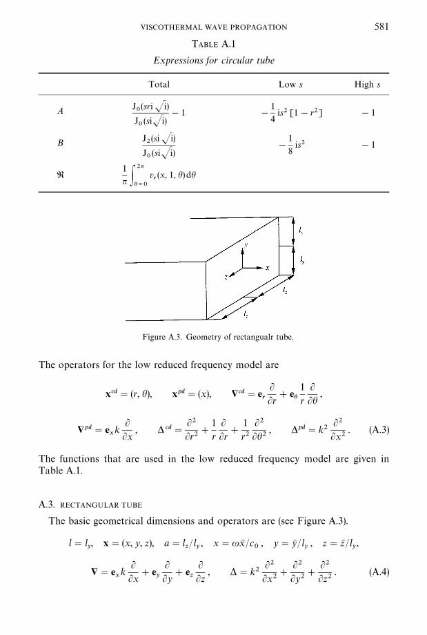
TABLE A.1

Expressions for circular tube

Total Low s High s

A J0(sri Ji)

J0(siJi)

!1 !

1

4is2 [1!r2] !1

B J2(si Ji)

J0(siJi)

!

1

8is2 !1

R1

n P2n

h/0

vr(x, 1, h)dh

Figure A.3. Geometry of rectangualr tube.


The operators for the low reduced frequency model are

xcd"(r, h), xpd"(x), $cd"er

LLr

#eh1r

LLh

,

$pd"exk

LLx

, * cd"L2

Lr2#

1r

LLr

#

1r2

L2

Lh2, *pd"k2

L2

Lx2. (A.3)

The functions that are used in the low reduced frequency model are given inTable A.1.

A.3. RECTANGULAR TUBE

The basic geometrical dimensions and operators are (see Figure A.3).

l"ly, x"(x, y, z), a"l

z/ l

y, x"uxN /c

0, y"yN / l

y, z"zN /l

y,

$"exk

LLx

#ey

LLy

#ez

LLz

, *"k2L2

Lx2#

L2

Ly2#

L2

Lz2. (A.4)

TABLE A.2

Expressions for rectangular tube

Total Low s High s

A Q1

=+

q/1,3. . .

(!1)q~12

qQ22Ccosh (Q

2z)

cosh (Q2)!1D cos A

qny

2 B Q1

=+

q/1,3. . .

(!1)q~12

qQK 22Ccosh (QK

2z )

cosh (QK2)!1D cos A

qny

2 B !1

Q1"

ia2s24

n; Q

2"aSA

qn2 B

2#is2 Q

1"

ia2s24

n; QK

2"a

qn2

B Q1

=+

q/1,3. . .

(!1)q~12

q2Q22Ctanh(aQ

2)

aQ2

!1D Q1

=+

q/1,3. . .

(!1)q~12

q2QK 22Ctanh(aQK

2)

aQK2

!1D !1

Q1"

ia2s28

n2; Q

2"aSA

qn2 B

2#is2 Q

1"

ia2s28

n12; QK

2"a

qn2

R1

4 P1

z/~1

[vy(x, 1, z)!v

y(x, !1, z)] dz

#

1

4

1

a P1

y/~1

[vz(x, y, 1)!v

z(x, y, !1)] dy

582W

.M.B

EL

TM

AN

Figure A.4. Geometry of the circular layer.

TABLE A.3

Expressions for the circular layer

Total Low s High s

A cosh (sz Ji)

cosh (sJi)!1

1

2is2 C

1

3z2!1D !1

B tanh(s Ji)

sJi!1 !

1

3is2 !1

R1

2[v

z(x, y, 1)!v

z(x, y, !1)]



xcd"(y, z), xpd"(x), $cd"exk

LLx

, $pd"ey

LLy

#ez

LLz

,

Dcd"L2

Ly2#

L2

Lz2, Dpd"k2

L2

Lx2. (A.5)

The functions that are used in the low reduced frequency model are given inTable A.2.

A.4. CIRCULAR LAYER


l"h0, x"(r, h, z), r"urN /c

0, h"hM , z"zN /h

0,

$"erk

LLr

#ehk1r

LLh

#ez

LLz

, D"k2L2

Lr2#k2

1r

LLr

#k21r2

L2

Lh2#

L2

Lz2. (A.6)


xcd"(z), xpd"(r, h), $cd"ez

LLz

, $pd"erk

LLr#ehk

1r

LLh

,

Dcd"L2

Lz2, Dpd"k2

L2

Lr2#k2

1r

LLr

#k21r2

L2

Lh2. (A.7)

Figure A.5. Geometry of the rectangular layer.

TABLE A.4

Expressions for the rectangular layer

Total Low s High s

A cosh(sz Ji)

cosh (sJi)!1

1

2is2 C

1

3z2!1D !1

B tanh(s Ji)

sJi!1 !

1

3is2 !1

R1

2[v

z(x, y, 1)!v

z(x, y, !1)]

584 W. M. BELTMAN

The functions that are used in the low reduced frequency model are given in TableA.3.

A.5. RECTANGULAR LAYER


l"h0, x"(x, y, z), a"l

y/l

x, x"uxN /c

0, y"uyN /c

0, z"zN /h

0,

$"exk

LLx

#eyk

LLy

#ez

LLz

, (A.8)

D"k2L2

Lx2#k2

L2

Ly2#

L2

Lz2. (A.9)


xcd"(z), xpd"(x, y), $cd"ez

LLz

, $pd"exk

LLx

#eyk

LLy

,

Dcd"L2

Lz2, Dpd"k2

L2

Lx2#k2

L2

Ly2. (A.10)

The functions that are used in the low reduced frequency model are given in TableA.4.


APPENDIX B: NOMENCLATURE

A function describing velocity and temperature pro"lesA

aq, B

aq, A

hq, B

hqconstants

Acd dimensionless cross-sectional areaLAcd dimensionless area of cross-section boundaryB(s) function accounting for viscous or thermal e!ectsa"l

y/ l

xaspect ratio

C function describing the temperature pro"leC

pspeci"c heat at constant pressure

Cv

speci"c heat at constant volumec0

undisturbed speed of soundD function describing the temperature pro"leen

unit normal vectorer

unit vector in the r directionex

unit vector in the x directioney

unit vector in the y directionez

unit vector in the z directioneh unit vector in the h directione/ unit vector in the / directionh0

half-layer thicknessi"J!1 imaginary unitjn

spherical Bessel function of order nJm

Bessel function of the "rst kind, order mk"ul/c

0reduced frequency

ka

acoustic wave numberkh

entropic wave numberkv

rotational wave numberl characteristic length scalelx

half-length in the x directionly

half-length in the y directionlz

half-length in the z directionn(sp) polytropic constantpN "p

0[1#pe*ut] pressure

p0

mean pressurep dimensionless pressure amplitudeR radiusR squeeze termR

0gas constant

rN radial co-ordinater dimensionless radial co-ordinates"lJo

0u/k shear wave number

¹M "¹0

[1#¹e*ut] temperature¹

0mean temperature

¹ dimensionless temperature amplitude¹

aacoustic temperature

¹h

entropic temperaturet timev6 "c

0ve*ut velocity vector

v dimensionless amplitude of the velocity vectorv dimensionless amplitude of the velocityvl

solenoidal velocity vectorvla

acoustic part of selenoidal velocity vectorvlh

entropic part of selenoidal velocity vector

586 W. M. BELTMAN

vv

rotational velocity vectorvr

dimensionless velocity component in the r directionvx

dimensionless velocity component in the x directionvy

dimensionless velocity component in the y directionvz

dimensionless velocity component in the z directionvh dimensionless velocity component in the h directionv/ dimensionless velocity component in the / directionvcd velocity vector in the cd directionsvpd velocity vector in the pd directionsx spatial co-ordinatesxcd cross-sectional co-ordinatesxpd propagation co-ordinatesC propagation constantc"C

p/C

vratio of speci"c heats

g bulk viscosityhM co-ordinate in the h directionh dimensionless co-ordinate in the h directionK

aconstant

Kh

constantj thermal conductivityk dynamic viscositym viscosity ratiooN "o

0[1#oe*ut] density

o0

mean density of airo dimensionless density amplitudep"JkC

p/j square root of the Prandtl number

U viscous dissipation function/M co-ordinate in the / direction/ dimensionless co-ordinate in the / directionu angular frequency$1 gradient operator$ dimensionless gradient operator$cd dimensionless gradient operator in the cd directions$pd dimensionless gradient operator in the pd directionsDM Laplace operatorD dimensionless Laplace operatorDcd dimensionless Laplace operator in the cd directions

Documents

VISCOTHERMAL WAVE PROPAGATION INCLUDING ACOUSTO …bctill/papers/numacoust/Beltman_19… · · 2009-07-13In tribology, the Reynolds ... the dimensions and the wavelength have to