Viscovery: A Platform for Trend Tracking in Opinion … A Platform for Trend Tracking in Opinion Forums WISDOM’17, August 2017, Halifax, Nova Scotia, Canada level per each sentiment

Viscovery: A Platform for Trend Tracking in Opinion ForumsIgnacio Espinoza

NovavizAv. Vicuña Mackenna 3939,

San JoaquínSantiago, Chile

[email protected]

Marcelo MendozaUniversidad Técnica Federico Santa

MaríaAv. Vicuña Mackenna 3939,

San JoaquínSantiago, Chile

[email protected]

Pablo OrtegaNovaviz

Av. Vicuña Mackenna 3939,San Joaquín

Santiago, [email protected]

Daniel RiveraNovaviz



Fernanda WeissNovaviz



ABSTRACTOpinions in forums and social networks are released by millionsof people due to the increasing number of users that use Web 2.0platforms to opine about brands and organizations. For enterprisesor government agencies it is almost impossible to track what peoplesay producing a gap between user needs/expectations and organiza-tions actions. To bridge this gap we create Viscovery, a platform foropinion summarization and trend tracking that is able to analyzea stream of opinions recovered from forums. To do this we usedynamic topic models, allowing to uncover the hidden structure oftopics behind opinions, characterizing vocabulary dynamics. Weextend dynamic topic models for incremental learning, a key as-pect needed in Viscovery for model updating in near-real time. Inaddition, we include in Viscovery sentiment analysis, allowing toseparate positive/negative words for a specific topic at differentlevels of granularity. Viscovery allows to visualize representativeopinions and terms in each topic. At a coarse level of granularity,the dynamic of the topics can be analyzed using a 2D topic em-bedding, suggesting longitudinal topic merging or segmentation.In this paper we report our experience developing this platform,sharing lessons learned and opportunities that arise from the use ofsentiment analysis and topic modeling in real world applications.

CCS CONCEPTS• Information systems→ Sentiment analysis; Retrieval tasksand goals;

KEYWORDSSentiment analysis, topic modeling, opinion platforms

Permission to make digital or hard copies of part or all of this work for personal orclassroom use is granted without fee provided that copies are not made or distributedfor profit or commercial advantage and that copies bear this notice and the full citationon the first page. Copyrights for third-party components of this work must be honored.For all other uses, contact the owner/author(s).WISDOM’17, August 2017, Halifax, Nova Scotia, Canada© 2017 Copyright held by the owner/author(s).ACM ISBN 978-x-xxxx-xxxx-x/YY/MM. . . $15.00https://doi.org/10.1145/nnnnnnn.nnnnnnn

ACM Reference format:Ignacio Espinoza, Marcelo Mendoza, Pablo Ortega, Daniel Rivera, and Fer-nanda Weiss. 2017. Viscovery: A Platform for Trend Tracking in OpinionForums. In Proceedings of ACM WISDOM jointly with KDD, Halifax, NovaScotia, Canada, August 2017 (WISDOM’17), 10 pages.https://doi.org/10.1145/nnnnnnn.nnnnnnn

1 INTRODUCTIONThe emergence of the Web 2.0 has allowed that millions of userscan send posts and opinions about celebrities, institutions, orga-nizations and brands. As the volume of opinions in forums andblogs increases, the need to develop effective platforms for opinionsearch has become urgent. In the stream of opinions, trend track-ing is a key building block of this kind of platforms, allowing todescribe what users expect about institutions/organizations andhow opinion trends evolve over time.

Effective tools for opinion browsing need to incorporate opinionaggregation functionalities, being relevant to obtain descriptions ofeach trend. In addition, the sentiment orientation of opinions w.r.t.named entities lights up how users act/react in front of a givenorganization. Sentiment analysis methods are helpful in this task.

As the volume of opinions is huge, the need to develop effectiveaggregation methods over opinions is the key building block of anyopinion trend platform. Opinion clustering is a way to aggregateopinions. Using hard clustering algorithms each opinion can beassigned to a single class. However, documents achieve a best de-scription by modeling its content with a mixture of topics, whereeach topic is defined as a probability distribution over words. Inthis way, opinions belong to several topics with different degreesof membership. This is the reason why documents are in generalmodeled using mixed membership models, an in particular LatentDirichlet Allocation (LDA) models [2], allowing to uncover thehidden structure of topics behind a corpus. LDA has made improve-ments in information retrieval tasks [10] and outperforms standardtext clustering algorithms being the state-of-the-art method fordocument aggregation.

https://doi.org/10.1145/nnnnnnn.nnnnnnn

https://doi.org/10.1145/nnnnnnn.nnnnnnn

WISDOM’17, August 2017, Halifax, Nova Scotia, Canada I. Espinoza et al.

In Chile, the National Agency of Consumers 1 centralize com-plaints about brands and their products. As it is almost impossibleto follow each complaint, consumers may be disappointed due tothe slow response of the Agency to their needs. To bridge this gapwe created Viscovery, a platform for opinion aggregation and trendtracking that allow to browse a huge volume of opinions in a fewminutes. The core of Viscovery is based on Dynamic Topic Models(DTM) [1], an extension of LDA [2] capable of model a time slicedcorpus, being able to estimate dependencies between vocabulariesacross time slices. To create Viscovery, we had to develop an in-cremental learning component able to update a model with newopinions. Our DTM update method achieves very similar resultsto DTM batch fitting in terms of topic coherence diminishing com-putational costs. In addition, we included in Viscovery sentimentanalysis. Sentiment analysis allows to distinguish between sub-jective/neutral terms in each distribution of words, enlighteninghow consumers opine about brands and products. To include sen-timent analysis in DTM we explore a simple approach based onaggregation, using lexical analysis at opinion level and conductingsentiment aggregations at topic and document level. A third ele-ment included in Viscovery is topic embedding. Using a time sliced2D topic embedding, topic merging and topic segmentation are sug-gested. Dynamics across topics are very interesting for the analysis,and is a promising characteristic of Viscovery that allow practition-ers to understand how topics evolve. Specific contributions of thepaper are:

• A scalable implementation of DTM for online training up-dating model parameters when new opinions come to theplatform.

• A simple way to incorporate sentiment analysis into DTM,allowing to explore neutral/subjective words at differentlevels of aggregation.

• A topic visualization tool that works with a time sliced 2Dtopic embedding, allowing to visualize how topics evolveover time.

The rest of the paper is organized as follows. In Section 2 wereview relatedwork on topicmodels and sentiment analysis. Section3 presents the architecture of Viscovery. Implementation issues arediscussed in Section 4. Incremental learning on DTM is presented inSection 5 and browsable sentiment analysis is discussed in Section6. Viscovery data slices are presented in Section 7 and finally weconclude in Section 8 giving conclusions and discussing futurework.

2 RELATEDWORKTopic models. Main efforts on topic models start with proba-

bilistic Latent Semantic Analysis [7] (pLSA), an aspect model fortext developed using topic mixtures. This approach decomposesa corpus of documents across terms introducing latent variables,decoupling terms and documents with topic mixtures. Model fit-ting was conducted using the Expectation-Maximization algorithm(EM) [3] casted for matrix completion with incomplete data. Asthe term-space is a high dimensional feature space, pLSA needsa high amount of data to perform well. As in general, text data issparse, pLSA tends to overfit limiting generalization capabilities. To1Sernac: Servicio Nacional del Consumidor, http://www.sernac.cl

tackle this problem, Blei et al. [2] introduced Dirichlet priors on vo-cabulary and document topic proportions. Using smoothing thesemodels addressed the over-fitting limitations of pLSA. This kind ofmodels, known as Latent Dirichlet Allocation (LDA) were firstly fit-ted using variational EM (VEM), an extension of the EM algorithmthat successfully handle incomplete data with distributional priors.Later, Griffiths and Steyvers [6] explored Gibbs sampling for LDAmodel fitting, reducing the number of iterations until convergence.Gibbs sampling is the standard method used for LDA model fittinguntil today because its fast convergence does not affect the qualityof the estimated models. Dynamic Topic Models (DTM) [1] wasintroduced to deal with vocabulary dynamics. DTM works over acorpus with timestamps, whilst model fitting is conducted usingtime slices of the corpus. Temporal dependencies across vocabular-ies are modeled using Kalman filtering, allowing to detect changesin descriptive words along different corpus slices. The inclusionof Kalman filtering in LDA for text dynamics involves additionalcomputational costs in model fitting, slowing convergence. Despitecomputational costs involved inmodel fitting, DTM can successfullyhandle text dynamics.

Sentiment analysis and topic modeling. A topic generative modelfor sentences with polarity was proposed by Eguchi and Lavrenko[4]. The model distinguishes between neutral words and sentimentwords using a random binary variable that controls the member-ship of each word to each one of the vocabularies. As documentscan be generated from sentiment or topic words, each sentenceachieves a polarity orientation calculated in terms of the numberof sentiment words that contains. Dirichlet smoothing was used ontopic and sentiment word distributions to avoid over-fitting. Theperformance of the model in information retrieval is tested infer-ring topic and sentiment orientation of each query showing thatthe proposal is feasible. Mei et al. [12] proposed Topic SentimentMixture (TSM), a sentiment topic model with a two tier mixture ofvocabularies to produce sentiment oriented sentences in a corpus.A first tier of the model is composed by neutral term distributions(one per each topic) and two additional term distributions for pos-itive and negative words. Then, each topic can be produced by amixture of these vocabularies defined from document proportions.The model is non-parametric (no distributional priors were used)and model fitting was conducted using the EM algorithm. TSM canbe considered as an extension of pLSA to sentiment analysis beingthe main difference the split conducted over the vocabulary to dis-tinguish between factual/subjective sentences. The Joint SentimentTopic model (JST) based on LDA was proposed by Lin and He [11].Term distributions were sampled over a simplex over terms crosspolarities, then the generative model drawn topic proportions con-ditioned on each polarity. In this way, words can be drawn by topics× polarities distributions, producing words by the joint effect oftopics and polarities in the document. As a consequence, sentimentcoverages at document level can be directly estimated by the model.JST is able to successfully address the sentiment classification taskat document level. An extension of JST was proposed by Jo andOh [9], who introduced Aspect and Sentiment Unification (ASUM).As JST, ASUM jointly models sentiments and topics, being topicproportions conditioned on polarities, with vocabularies at topic

Viscovery: A Platform for Trend Tracking in Opinion Forums WISDOM’17, August 2017, Halifax, Nova Scotia, Canada

level per each sentiment orientation. However, ASUM models sen-timent at sentence level, with words conditioned at a single topicper sentence. Results on sentiment classification shows that ASUMoutperforms JST and comes close to supervised methods whilstASUM does not require labels for model fitting. The state of the artshows that main efforts on sentiment topic modeling are focusedon static models, discarding vocabulary dynamics. As the core ofViscovery is DTM, we will need to use a different approach to in-clude sentiment analysis into dynamic topic models. We will showin Section 6 how we use sentiment analysis at sentence level toconduct aggregation at different levels of granularities over DTM.

3 VISCOVERY: ARCHITECTURE ANDDESIGN PRINCIPLES

In this section we discuss how we integrate different algorithmsto ingest/process/aggregate opinions into Viscovery. We modeldifferent algorithms as micro services to develop a platform fortrend tracking in opinion forums. A micro service architectureorganizes the platform as a set of weakly coupled services whereeach service implements a set of encapsulated procedures. Forexample, a micro service in Viscovery corresponds to an indexer ofopinionated tweets. Services in Viscovery are communicated usingasynchronous protocols. We developed each service independentlyof the other. Indeed each micro service has its own database inorder to be decoupled from other services.

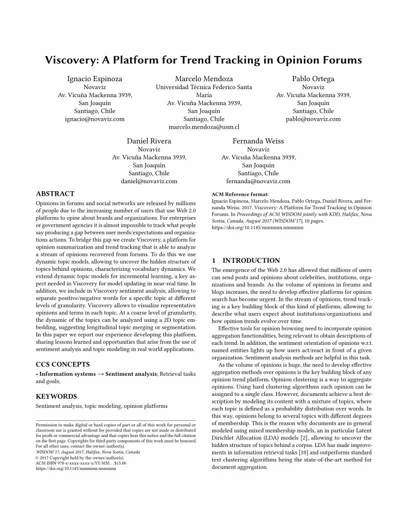
To develop Viscovery we create a start-up named Novaviz. Theidea behind Novaviz is to develop tools for text data management.To accomplish this purpose we develop the Novaviz API Gateway, alist of services and functionalities implemented in Python, requestedby four components: a) Data Ingester, b) Data Preprocessor, c) DataProcessor, and d) Indexer. For visualization we use three libraries: a)DFR browser, b) Kibana, and c) D3. Visualization and processes areconnected through micro services defined in Novaviz API Gateway,as is shown in the architectural diagram of Figure 1.

Data Ingester. This component is in charge of opinion recollec-tion from heterogeneous sources as Twitter and web forums (e.g.http://www.reclamos.cl). It calls services from the Novaviz API.Among the services requested the most important is web scrapping,that allows Viscovery to retrieve opinions from web page forums.For storage, this component interacts with Redis 2, an open source(BSD licensed) in-memory data structure store, used as a cachedatabase to support this process.

Preprocessor. This component normalize the text. It calls servicesfrom the Novaviz API as stopwords removal, caps normalizationand symbol/punctuation removal. It allows Viscovery to create avocabulary of keywords to describe opinions by content. For storagethis component interacts with MongoDB 3, a noSQL database fordocument storage and retrieval.

Processor. This component is in charge of text analysis and isthe core component of Viscovery. It calls services from the No-vaviz API as Dynamic Topic Models and Sentiment Analysis. ForDynamic Topic Models (DTM), the API wraps Gensim 4. Gensim2https://redis.io/3https://www.mongodb.com/4http://radimrehurek.com/gensim/

is an implementation of topic modeling written in Python [13]. Itincludes implementations of LDA, LSI and DTM. For sentimentanalysis, the API wraps Vader 5, a rule-based model for sentimentanalysis that uses a lexicon of English words [8]. As the preproces-sor component, the processor interacts for storage with MongoDB,allowing to register each view of the data (e.g. topic model view) asa document view of each opinion, with the attributes leveraged bythe respective view. For instance, from the sentiment view of anopinion, each document in MongoDB stores neutral, positive andnegative scores at sentence level. Weights for topic membership arestored in the topic model view of each opinion. Then, documentsin MongoDB will ingest the indexer, the component that providesdata for opinion search and browsing.

Indexer. This component is in charge of opinion indexing. Foreach view of the data, we create an index allowing search andbrowsing at different levels of granularity. As opinions are clus-tered using topic models, browsing is conducted using topics asopinion aggregation containers. For each topic, each opinion regis-ter its membership score, which indicates the degree of membershipof each opinion to the topic. As each topic is a probability distri-bution over words, we store the weights of each word per topic.As browsing is conducted over topics, the use of words to describeeach topic is a key element of Viscovery. To integrate the sentimentview of the data, we index opinions and their related sentimentweights for search and browsing. To ingest these indexes, we re-cover the document views created by the processor in the previousstep, processing and indexing them into Elasticsearch 6. Elastic-search is a distributed, RESTful search and analytics engine capableof support searches over unstructured data implementing fast andefficient data access operations using inverted indexes. We use Elas-ticsearch indexes to support all the search and browsing operationsin Viscovery.

DFR browser. To visualize opinion trends we started using DFRbrowser 7, a visualization tool that works over topic models to inte-grate data views into a single, coherent, and searchable visualizationof the data. As the code of DFR browser is available, we startedworking over DFR browser to cast this tool to our needs and re-quirements. DFR allows to search over topics, the basic search-ableelement in the visualization, and to disaggregate the informationat topic level into documents and words by topic.

Kibana. Kibana is part of the suite provided by Elastic, namedThe Open Source Elastic Stack. The purpose of Kibana is to handElaticsearch visualizations.

D3.js. Another tool that we use for data visualizations is D3.js8. D3.js is a JavaScript library for data visualizations compatiblewith HTML, SVG, and CSS. D3 follows a data-driven approachfor data manipulation, using DOM as a standard for documentrepresentation.

5https://github.com/cjhutto/vaderSentiment6https://www.elastic.co/7https://agoldst.github.io/dfr-browser/8https://d3js.org/


Figure 1: Viscovery architectural diagram. Visualization components are connected to data processing components using theNovaviz API.

4 IMPLEMENTATION ISSUES4.1 Novaviz APIThe Novaviz API includes a list of services and functionalities. Asthe architecture of Viscovery is micro service oriented, the NovavizAPI contains a list of reusable and generic services. Our API includesseven services:

Scrapper. This service extracts and recovers data from heteroge-neous data sources as Twitter or opinionweb forums (e.g. reclamos.cl).In the case of Twitter, it takes as seed a hashtag using the publicAPI and producing a .json file compounded by the list of tweets thatcontains the hashtag. In the case of reclamos.cl we scrap the htmlsource code of the forum recovering a semi-structured view of theforum in a .json file. The attributes included in the file are creationdate, the complaint content (unstructured), the url (a permalinkcreated by reclamos.cl for each opinion), and the title of the com-plaint. It is implemented using Scrapy 9, a scrapper implementedin Python. The scrapper is called by the ingester component ofViscovery.

Corpus constructor. It takes scrapper outputs in .json format pre-processing the content to normalize the text. It starts tokenizing thetext. Is in this service that caps, stopwords, accents, punctuationand symbols are processed. We include a rule-based word removalby frequency. By default, words with one occurrence in the data areremoved. In addition, a second rule-based word removal is included,removing words by length. Words with less than two chars are re-moved from the vocabulary. The constructor is language-flagged.Novaviz considers two languages, English and Spanish. By default,9https://scrapy.org/

the constructor is set to English. The stopword list is customizable.In addition, the basis for time slicing can be defined here using aparameter with values in {daily,weekly,monthly, yearly}. Out-put files produced by the corpus creator are foo.dict (dictionary),foo.lda-c (a row oriented file with one doc per row and entries in-dicating word occurrences), sliced.json (docIDs and timestamps).These files are used for LDA model fitting. The corpus constructoris called by the preprocessor component of Viscovery.

LDA fitting. It takes foo.dict (dictionary) and foo.lda-c for LDAmodel fitting. It needs the number of topics as a parameter (fivetopics by default). LDA fitting wraps the Gensim implementation ofLDA that is based on Gibbs sampling [6]. Output files produced byLDA fitting are stored in a directory that contains topic-word.json(truncated to the top-30 words per topic), doc-topic.json (topicproportions), frequency.txt (a list of words with their occurrencesof the corpus), and foo which corresponds to the model file, a codedview of the fitted model. LDA fitting is called by the processorcomponent of Viscovery.

DTM fitting. Analogously to LDA fitting, this service wraps theGensim implementation of DTM. It takes foo.dictionary, foo.lda-cand sliced.json for DTM fitting. Output files produced by DTM aretopic-word.json with timestamps (one timestamp per time slice foreach word in the dictionary), doc-topic.json (topic proportions),frequency.txt, and foo which corresponds to the coded view of theDTM model. DTM fitting is called by the processor component ofViscovery.

Sentiment Analysis. It takes the .json file produced by the Scrap-per and conducts sentiment analysis using VADER. It works at


three different levels of granularity, sentences, documents and top-ics. Output files produced by Sentiment Analysis are stored in .jsonfiles (with pairwise entries ID-sentiment score). A detailed discus-sion about how sentiment scores are calculated at different levelsof granularity is provided in Section 6.

NER. It takes the .json file produced by the Scrapper service,and conducts named entity recognition using NLTK 10 (NaturalLanguage ToolKit, a Python implementation of NLP basic tools).Output files produced by NER are stored in .json files (with pairwiseentries wordID-NER tag).

POS. It takes the .json file produced by the Scrapper service, andconducts part-of-speech using NLTK. Output files produced by POSare stored in .json files (with pairwise entries wordID-POS tag).

Topic scaling. It takes as input the foo model file retrieved fromLDA fitting. In addition it takes the foo.dict (dictionary) and foo.lda-cfrom corpus constructor to recover document lengths. Topic scalingwraps Principal Coordinate Analysis (PCoA) using the implemen-tation provided in Scikit-bio 11. Dimensionality reduction is con-ducted using PCoA towards a 2D embedding based on the Jensen-Shannon divergence between topics. The output file produced bytopic scaling is a .json file with paiwise entries topicID - ⟨x, y⟩.Topic scaling is called by DFR browser for topic visualization.

4.2 Elastic IndexesFor data storage we use Elastisearch indexes. Elasticsearch providesservices for data indexing and retrieval. Elastic indexes are keyelements for opinion browsing, allowing to browse opinions atdifferent levels of granularity. For each level of granularity wecreated a specific index in Elastic:

Opinions index. This index retrieves opinions using a docID as asearch key. Each opinion is indexed at full content, allowing fastretrieval of opinions when documents are picked in Viscovery.

Topic-word index. This index retrieves top-K words per topic,using topicID as a search key. For each word the index stores themembership level for the topic.

Topic-document index. This index retrieves top-k documents pertopic, using topicID as a search key. For each document the indexstores the membership level for the topic.

Term frequency index. This index retrieves the frequency of eachterm using termID as a search key.

Sentiment-document index. This index retrieves sentiment scoresat document level using docID as a search key.

Sentiment-topic index. This index retrieves sentiment scores attopic level using topicID as a search key.

Sentiment-sentence index. This index retrieves sentiment scoresat sentence level using sentenceID as a search key.

10http://www.nltk.org/11http://scikit-bio.org/

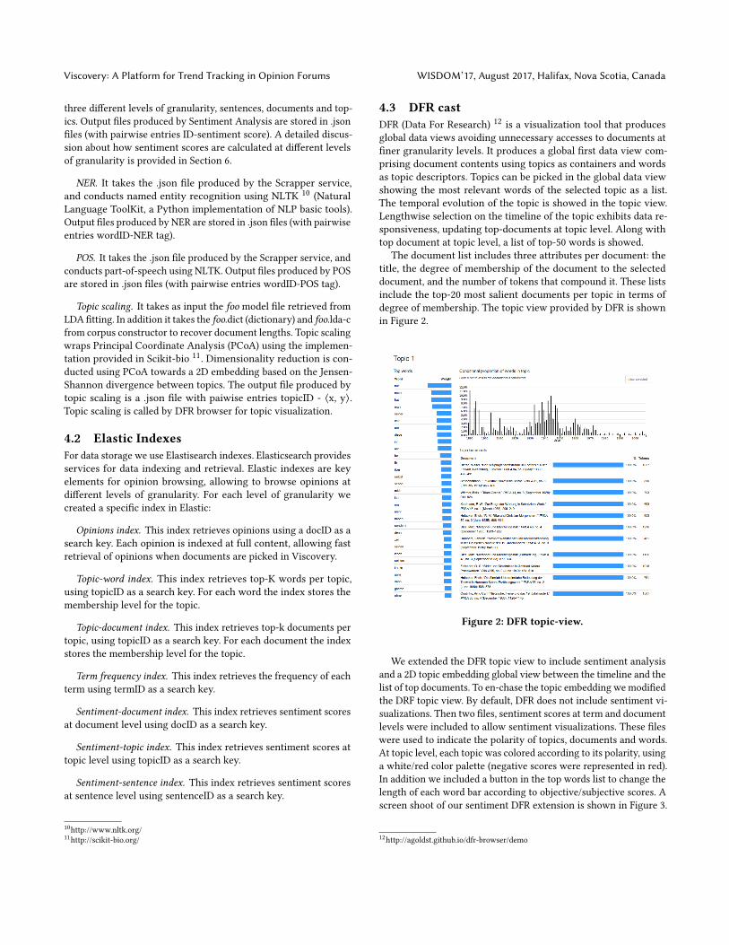
4.3 DFR castDFR (Data For Research) 12 is a visualization tool that producesglobal data views avoiding unnecessary accesses to documents atfiner granularity levels. It produces a global first data view com-prising document contents using topics as containers and wordsas topic descriptors. Topics can be picked in the global data viewshowing the most relevant words of the selected topic as a list.The temporal evolution of the topic is showed in the topic view.Lengthwise selection on the timeline of the topic exhibits data re-sponsiveness, updating top-documents at topic level. Along withtop document at topic level, a list of top-50 words is showed.

The document list includes three attributes per document: thetitle, the degree of membership of the document to the selecteddocument, and the number of tokens that compound it. These listsinclude the top-20 most salient documents per topic in terms ofdegree of membership. The topic view provided by DFR is shownin Figure 2.

Figure 2: DFR topic-view.

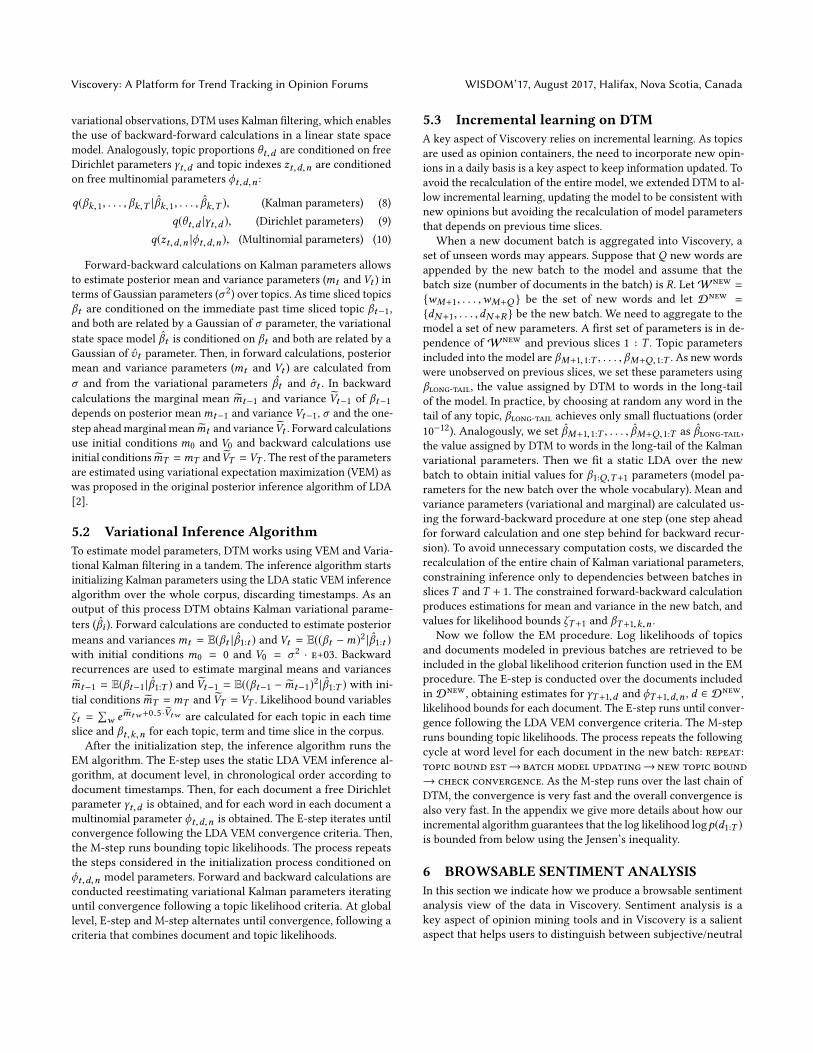
We extended the DFR topic view to include sentiment analysisand a 2D topic embedding global view between the timeline and thelist of top documents. To en-chase the topic embedding we modifiedthe DRF topic view. By default, DFR does not include sentiment vi-sualizations. Then two files, sentiment scores at term and documentlevels were included to allow sentiment visualizations. These fileswere used to indicate the polarity of topics, documents and words.At topic level, each topic was colored according to its polarity, usinga white/red color palette (negative scores were represented in red).In addition we included a button in the top words list to change thelength of each word bar according to objective/subjective scores. Ascreen shoot of our sentiment DFR extension is shown in Figure 3.

12http://agoldst.github.io/dfr-browser/demo


Figure 3: Sentiment DFR topic-view.

5 INCREMENTAL LEARNING FOR DYNAMICTOPIC MODELS

5.1 Dynamic Topic ModelsA set of latent variables can be introduced to model the relation-ships between terms and documents in a corpus. Formally, letd ∈ D = {d1,d2, . . . ,dN } and w ∈ W = {w1,w2, . . . ,wM } berandom variables representing documents and terms, respectively.A set of random variables z ∈ Z = {z1, z2, . . . , zk } can be in-troduced to model the joint probability of documents and terms,producing a mixed membership model expressed as follows:

P(w |d) =∑z∈Z

P(w |z) · P(z |d). (1)

Using the Bayes rule to invert the conditional probability P(z |d),we obtain an expression of the joint probability conditioned to themodel parameters:

P(w,d) =∑z∈Z

P(w |z) · P(d |z) · P(z). (2)

The equation 2 is known as the generative formulation of the topicmodel of the corpus.

Topic models based on Dirichlet allocation require two Dirichletdistributions. A first one generates topic proportions for each doc-ument and a second one generates terms conditioned on documenttopics proportions. Specifically, a Dirichlet k-dimensional randomvariable θ takes values in a k-1 simplex (0 ≤ θi ≤ 1,

∑ki=1 θi = 1),

where its density function is defined by:

p(θ |α) =Γ(∑k

i=1 αi )∏ki=1 Γ(αi )

θα11 · . . . · θαkk , (3)

and {α1, . . . ,αk } corresponds to the distributional parameters,αi >0. Then, equation 2 is expanded using Dirichlet priors:

P(W ,d) =M∏n=1

P(wn |zn , β) · P(zn |θd ) · P(θd |α). (4)

In equation 4, θd indicates the proportion of topics in d . Then,zn is conditioned on β and represents the sampling probabilityof wn on d . Note that α and β are the distributional parametersof the Dirichlet density functions. Usually they are consigned ashyper-parameters to make a difference with model parameters. Itis common to make an assumption of density symmetry for hyper-parameters, that is α1 = . . . = αk = α and β1 = . . . = βk = β . Thevalues α , β control the level of smoothness/sharpness of the densityfunctions around the centroid of the simplex.

To model a time sliced corpus, Blei and Lafferty [1] introduceddynamic topic models (DTM). DTM is based on the static LatentDirichlet Allocation model and use the mean parameterizationof the multinomial topic distribution. The idea behind DTM is touse the mean parameterization of the topics to introduce meanchaining, being possible to model time dependencies over time. Tochain topics over time, DTM models the chain of mean parametersintroducing Gaussian noise, modeling uncertainty over time slices.Let βt,k be the k-th topic in the time slice t and let π be the meanparameter of the topic. Note that the i-th component of βt,k is givenby βi = log

(πiπV

). As πi represents the expected value of wi and

πV is the expected value of a random chosen word over the wholevocabulary V , the fraction πi

πV is the odd ofwi over V and then βicorresponds to the logit function forwi overV . As is known, a zerovariation overV achieves a zero value in the logit function. Positiveor negative deviations of wi in V achieves positive or negativevalues in [−1,+1], respectively. Then, βt,k can be chained in a statespace of parameters that evolves with Gaussian noise:

βt,k |βt−1,k ∼ N(βt−1,k ,σ 2I). (5)

Topic proportions are also chained in DTM, using mean parame-terization over θ :

θt |θt−1 ∼ N(αt−1,δ2I). (6)

Time chaining does not affect model expressiveness. In fact, thedecomposition of the joint distribution of words and documents ina corpus remains the same, except for the fact that both Dirichletdistributions (on topic proportions and terms) are conditioned onthe Dirichlet distributions of the previous time slice:

P(W ,d, t) =M∏n=1

P(wn |zn , βt ) · P(zn |θd,t ) · P(θd,t |α). (7)

Model estimation has some drawbacks under these assumptions.Posterior inference (model estimation of parameters conditionedon observed variables) is intractable due to the non conjugacy ofGaussians and multinomial distributions. Blei and Lafferty exploredvariational methods for posterior inference, discarding stochasticsimulation (e.g. Gibbs sampling) due to computational difficultiesinherent in the non conjugacy of Gaussians. To retain the sequentialstructure of topics over time, DTM fits a dynamic model with Gauss-ian variational observations (βk,1, . . . , βk,t , . . . , βk,T ), fitting theseparameters to minimize the Kullback-Leibler divergence betweenthe resulting posterior and the true posterior. To mimic Gaussian


variational observations, DTM uses Kalman filtering, which enablesthe use of backward-forward calculations in a linear state spacemodel. Analogously, topic proportions θt,d are conditioned on freeDirichlet parameters γt,d and topic indexes zt,d,n are conditionedon free multinomial parameters ϕt,d,n :

q(βk,1, . . . , βk,T |βk,1, . . . , βk,T ), (Kalman parameters) (8)q(θt,d |γt,d ), (Dirichlet parameters) (9)

q(zt,d,n |ϕt,d,n ), (Multinomial parameters) (10)

Forward-backward calculations on Kalman parameters allowsto estimate posterior mean and variance parameters (mt and Vt ) interms of Gaussian parameters (σ 2) over topics. As time sliced topicsβt are conditioned on the immediate past time sliced topic βt−1,and both are related by a Gaussian of σ parameter, the variationalstate space model βt is conditioned on βt and both are related by aGaussian of vt parameter. Then, in forward calculations, posteriormean and variance parameters (mt and Vt ) are calculated fromσ and from the variational parameters βt and σt . In backwardcalculations the marginal mean mt−1 and variance Vt−1 of βt−1depends on posterior meanmt−1 and varianceVt−1, σ and the one-step aheadmarginal mean mt and variance Vt . Forward calculationsuse initial conditions m0 and V0 and backward calculations useinitial conditions mT =mT and VT = VT . The rest of the parametersare estimated using variational expectation maximization (VEM) aswas proposed in the original posterior inference algorithm of LDA[2].

5.2 Variational Inference AlgorithmTo estimate model parameters, DTM works using VEM and Varia-tional Kalman filtering in a tandem. The inference algorithm startsinitializing Kalman parameters using the LDA static VEM inferencealgorithm over the whole corpus, discarding timestamps. As anoutput of this process DTM obtains Kalman variational parame-ters (βi ). Forward calculations are conducted to estimate posteriormeans and variancesmt = E(βt |β1:t ) and Vt = E((βt −m)2 |β1:t )with initial conditions m0 = 0 and V0 = σ 2 · e+03. Backwardrecurrences are used to estimate marginal means and variancesmt−1 = E(βt−1 |β1:T ) and Vt−1 = E((βt−1 − mt−1)2 |β1:T ) with ini-tial conditions mT =mT and VT = VT . Likelihood bound variablesζt =

∑w emtw+0.5·Vtw are calculated for each topic in each time

slice and βt,k,n for each topic, term and time slice in the corpus.After the initialization step, the inference algorithm runs the

EM algorithm. The E-step uses the static LDA VEM inference al-gorithm, at document level, in chronological order according todocument timestamps. Then, for each document a free Dirichletparameter γt,d is obtained, and for each word in each document amultinomial parameter ϕt,d,n is obtained. The E-step iterates untilconvergence following the LDA VEM convergence criteria. Then,the M-step runs bounding topic likelihoods. The process repeatsthe steps considered in the initialization process conditioned onϕt,d,n model parameters. Forward and backward calculations areconducted reestimating variational Kalman parameters iteratinguntil convergence following a topic likelihood criteria. At globallevel, E-step and M-step alternates until convergence, following acriteria that combines document and topic likelihoods.

5.3 Incremental learning on DTMA key aspect of Viscovery relies on incremental learning. As topicsare used as opinion containers, the need to incorporate new opin-ions in a daily basis is a key aspect to keep information updated. Toavoid the recalculation of the entire model, we extended DTM to al-low incremental learning, updating the model to be consistent withnew opinions but avoiding the recalculation of model parametersthat depends on previous time slices.

When a new document batch is aggregated into Viscovery, aset of unseen words may appears. Suppose that Q new words areappended by the new batch to the model and assume that thebatch size (number of documents in the batch) is R. LetWnew ={wM+1, . . . ,wM+Q } be the set of new words and let Dnew ={dN+1, . . . ,dN+R } be the new batch. We need to aggregate to themodel a set of new parameters. A first set of parameters is in de-pendence of Wnew and previous slices 1 : T . Topic parametersincluded into the model are βM+1,1:T , . . . , βM+Q,1:T . As new wordswere unobserved on previous slices, we set these parameters usingβlong-tail, the value assigned by DTM to words in the long-tailof the model. In practice, by choosing at random any word in thetail of any topic, βlong-tail achieves only small fluctuations (order10−12). Analogously, we set βM+1,1:T , . . . , βM+Q,1:T as βlong-tail,the value assigned by DTM to words in the long-tail of the Kalmanvariational parameters. Then we fit a static LDA over the newbatch to obtain initial values for β1:Q,T+1 parameters (model pa-rameters for the new batch over the whole vocabulary). Mean andvariance parameters (variational and marginal) are calculated us-ing the forward-backward procedure at one step (one step aheadfor forward calculation and one step behind for backward recur-sion). To avoid unnecessary computation costs, we discarded therecalculation of the entire chain of Kalman variational parameters,constraining inference only to dependencies between batches inslices T and T + 1. The constrained forward-backward calculationproduces estimations for mean and variance in the new batch, andvalues for likelihood bounds ζT+1 and βT+1,k,n .

Now we follow the EM procedure. Log likelihoods of topicsand documents modeled in previous batches are retrieved to beincluded in the global likelihood criterion function used in the EMprocedure. The E-step is conducted over the documents includedin Dnew, obtaining estimates for γT+1,d and ϕT+1,d,n , d ∈ Dnew,likelihood bounds for each document. The E-step runs until conver-gence following the LDA VEM convergence criteria. The M-stepruns bounding topic likelihoods. The process repeats the followingcycle at word level for each document in the new batch: repeat:topic bound est→ batch model updating→new topic bound→ check convergence. As the M-step runs over the last chain ofDTM, the convergence is very fast and the overall convergence isalso very fast. In the appendix we give more details about how ourincremental algorithm guarantees that the log likelihood logp(d1:T )is bounded from below using the Jensen’s inequality.

6 BROWSABLE SENTIMENT ANALYSISIn this section we indicate how we produce a browsable sentimentanalysis view of the data in Viscovery. Sentiment analysis is akey aspect of opinion mining tools and in Viscovery is a salientaspect that helps users to distinguish between subjective/neutral


information. As a base service, the Novaviz API uses VADER [8]for sentiment sentence tagging. VADER provides three sentimentscores at sentence level: positive (scs (⊕)), negative (scs (⊖)) andneutral (scs (⊙)) scores, where scs (⊕) + scs (⊖) + scs (⊙) = 1. Werecover for each sentence in our data these scores.

Document level. A first level of aggregation considered in Vis-covery is the document level. As opinions can be compounded bya number of sentences, sentiment scores need to be aggregatedat opinion level. Let d be a document indexed in Viscovery, ands ∈ d the sentences that compounds d , where |d | is the number ofsentences of d . Sentiment scores at document level are obtainedfrom:

scd (∗) =∑s ∈d

scs (∗)|d | , with ∗ ∈ {⊕, ⊖, ⊙} (11)

Note that scd (⊕) + scd (⊖) + scd (⊙) = 1, as expected.

Topic level. A second level of aggregation considered in Vis-covery is the topic level. As opinions are aggregated into topics,sentiment scores need to be aggregated at topic level to indicate thelevel of polarity of each topic. Let z be a LDA latent variable, andP(d |z) the membership probability given by DTM and defined inEquation 2. Note that P(∗|z) = ∑

d ∈D P(∗|d) · P(d |z). For simplicity,we denote P(∗|z) by scz (∗). Then, sentiment scores at topic levelare obtained from:

scz (∗) = Cz ·∑d ∈D

scd (∗) · P(d |z), with ∗ ∈ {⊕, ⊖, ⊙} (12)

where Cz = 1∑∗ scz (∗)

. Note that scz (⊕) + scz (⊖) + scz (⊙) = 1, asexpected.

Term level. At a high level of granularity Viscovery browsesterms. To use sentiment analysis at term level, we need to esti-mate P(∗|w), denoted for simplicity by scw (∗). As scw (∗) can beexpanded over latent variables by

∑z∈Z scz (∗) · P(z |w), using the

Bayes rule on P(z |w) we obtain scw (∗) as:

scw (∗) =∑z∈Z

scz (∗) ·P(w |z) · P(z)

P(w) , with ∗ ∈ {⊕, ⊖, ⊙} (13)

Note that scw (⊕) + scw (⊖) + scw (⊙) = 1, as expected.

Using topics as proxies. Viscovery allows to browse opinionsusing topics as proxies. When a topic is picked in Viscovery, thesentiment view of the data can be projected to documents or terms.To show sentiment scores conditioned on topics, we reuse thescores defined in equations 11-13. Sentiment scores at documentlevel conditioned on topics are defined by:

scd (∗|z) =( ∑w ∈W

scw (∗) · P(w |z))· P(z |d), with ∗ ∈ {⊕, ⊖, ⊙}

(14)Analogously, sentiment scores at term level conditioned on topics

are defined by:

scw (∗|z) =( ∑d ∈D

scd (∗) · P(d |z))· P(z |w), with ∗ ∈ {⊕, ⊖, ⊙}

(15)

This simple way to aggregate scores from sentence sentimentscores allows us to use sentiment analysis on DTM.

7 DATA SLICES AND PRELIMINARY RESULTSIncremental learning testingWe evaluate our incremental version of DTM to measure speed upand model quality in terms of topic coherence [14]. We expect toreduce the computational time involved in model fitting avoidinga retrogress in terms of topic coherence. To test this aspect of ourproposal, we run ten trials of model fitting for a corpus, with andwithout incremental learning on the last time slice. We used astest data a curated dataset to evaluate topic coherence provided byGreene & Cross [5] that comprises news about the political agendaof the European Parliament. The dataset is divided into four timeslices and is compounded by 1324 news articles classified into amanually-specified number of topics, helping to evaluate topic co-herence. Mean and variance of coherence and mean computationaltime involved in both algorithms are reported in Table 1.

Algorithm Mean Coh. Var Coh. Mean Comp. TimeDTM -1.5747 0.0047 2:06:56DTM + Seq. Upd. -1.5373 0.0063 1:47:37 + 0:11:50

Table 1: Topic coherence and computational times in DTMand DTM+seq update. Mean and variance over ten trials peralgorithm are reported.

As expected, the mean computational time involved in DTM +Seq. Upd. is less than the time registered by DTM, with only 11minutes spent in the fourth slice. This result indicate that the mostexpensive step of the algorithm is the Kalman variational inferenceand as our proposal constraints this step two the last slice, it reducesthe cost involved. As the data used for this experiment is small(we used this dataset to estimate topic coherence) the differencebetween both algorithms in terms computational time is small. InReclamos.cl, a big data set with more than 200,000 complains thatwe indexed in Viscovery, the difference between both algorithmsis high. If we use DTM over the whole dataset, model fitting takes14.7 hours. On the other hand, using sequential update over the lasttime slice it takes 1.91 hours. Note that without sequential update,we will need to retrain the whole model for each new slice and ourproposal avoids this with a speed up of almost 8x. Surprisingly thetime reduction does not affect the quality of the model in termsof topic coherence as is shown in Table 1. In fact, our proposalachieves a slight improvement over DTM at a cost of a highervariance between the different trials.

7.1 Data slices over Reclamos.clWe are developing Viscovery implementing new functionalities. Infact, the current version of Viscovery implements browsable senti-ment analysis at topic and word levels. Currently we are workingon the implementation of sentiment analysis at document level,according to the proposal introduced in Section 6. Viscovery allowsto browse opinions using topics as proxies of opinions. We indexedinto Viscovery 12 years of data from Reclamos.cl, a Chilean fo-rum for complaints abouts companies, marks and institutions. The


dataset contains 201,969 different complaints. Retail, government,banks and universities are among the most frequent subjects ofopinions.

The size of the vocabulary after stopword removal is 86,723 terms.We used 18 hours to create the corpus of reclamos using Viscovery.Reclamos.cl is a very active site in Chile, reporting an overall of90,128 persons contacted by companies after complaint publication(a significant number in proportion to the Chilean population).

Running DTM using years as timestamps, we achieved 12 timeslices of the data. We used the default value for the number of topics,set as 10 for this example. Data slices for this corpus are shown inFigure 4. As Figure 4 shows, the a) Corpus view (overview) has fouralternatives for corpus deployment: grid, scaled, list and stacked.We show topics using lists as data view. The list of topics includetopics proportions over time, topwords per topic and the proportionof the topic in the corpus. When a topic is selected (we click topic1 for this example), the b) Topic view is deployed. A topic viewshows the list of top words for the topic, sorted in decreasing orderaccording to the proportion on the topic. If the polarity bottom ispressed the bars are modified according to the sentiment weightof the word in the topic. For this version of Viscovery, the barsize is proportional to the sum of positive and negative scores.Currently we are implementing an extension that produces twobars per term, one per polarity. Topic embeddings are also shownin this view, illustrating the correlation of topic (distances in thetopic embedding). The polarity orientation of each topic is shownusing a color bar, where negative-biased topics are indicated withred shades. A list of top-documents per topic is shown below theembedding (omitted in this figure) and the user can select a specificopinion. In this case, Viscovery deploys the c) Document view,where the top words of the document in the given topic are shown.The subject and the date of the complaint is shown at the top ofthe view. Finally, Viscovery provides a d) Term view across topics,showing how relevant is a given word across topics. In the example,we show the word view using the term ’company’, and as expected,this word is used in many topics of reclamos.cl, with different levelsof membership.

8 CONCLUSIONSWe present Viscovery, a tool for opinion browsing and trend track-ing. Key elements of Viscovery are Dynamic Topic Models (DTM)and our extension of DTM for sequential updating. We includesentiment analysis in Viscovery starting from sentiment scores atsentence level and then, conducting aggregation across topics anddocuments. This approach is simple and effective. For visualizationwe use DFR browser, extending DFR to include topic embeddingsand sentiment analysis.

Currentlywe are extending Viscovery to includemore functional-ities. Among these functionalities we are working on the sentiment-document view, topic evolution tracking view and opinion searchmodule. We are implementing these modules using Kibana and D3,two visual components considered in Viscovery not included in thecurrent version. In addition, we are using Viscovery to index moresources, as opinions retrieved from Twitter and Reddit.

ACKNOWLEDGMENTThis work was supported by the Fondef VIU 15E0085 project of theNational Agency of Science and Technology, Conicyt, Chile.

REFERENCES[1] David Blei and John Lafferty. 2006. Dynamic topic models. In Proceedings of the

23rd International Conference on Machine Learning, ICML. 113–120.[2] David Blei, Andrew Ng, and Michael Jordan. 2003. Latent Dirichlet Allocation.

Journal of Machine Learning Research 3, 4-5 (2003), 993–1022.[3] Arthur Dempster, Nan Laird, and Donald Rubin. 1977. Maximum likelihood from

incomplete data via the EM algorithm. Journal of the Royal Statistics Society 39(1977), 1–38.

[4] Koji Eguchi and Victor Lavrenko. 2006. Sentiment retrieval using generativemodels. In Proceedings of the 6th Conference on Empirical Methods in NaturalLanguage Processing, EMNLP. 345–354.

[5] Derek Greene and James P. Cross. 2016. Exploring the Political Agenda ofthe European Parliament Using a Dynamic Topic Modeling Approach. CoRRabs/1607.03055 (2016).

[6] Thomas Griffiths and Mark Steyvers. 2004. Finding scientific topics. Proceedingsof the National Academy of Sciences, PNAS 101, 1 (2004), 5228–5235.

[7] Thomas Hofmann. 2001. Unsupervised learning by probabilistic latent semanticanalysis. Machine Learning 42, 2 (2001), 177–196.

[8] C.J. Hutto and Eric Gilbert. 2014. VADER: A Parsimonious Rule-based Model forSentiment Analysis of Social Media Text. In Proceedings of the Eighth InternationalConference on Weblogs and Social Media, ICWSM.

[9] Yohan Jo and Alice Oh. 2011. Aspect and sentiment unification model for onlinereview analysis. In Proceedings of the 4th ACM International Conference on WebSearch and Data Mining, WSDM. 815–824.

[10] Oren Kurland and Lillian Lee. 2009. Clusters, language models, and ad hocinformation retrieval. ACM Transactions on Information Systems, TOIS 27, 3(2009).

[11] Chenghua Lin and Yulan He. 2009. Joint sentiment/topic model for sentimentanalysis. In Proceedings of the 18th ACM International Conference on Informationand Knowledge Management, CIKM. 375–384.

[12] Qiaozhu Mei, Xu Ling, Matthew Wondra, Hang Su, and ChengXiang Zhai. 2007.Topic sentiment mixture: modeling facets and opinions in weblogs. In Proceedingsof the 16th ACM International World Wide Web Conference, WWW. 171–180.

[13] Radim Řehůřek and Petr Sojka. 2010. Software Framework for Topic Modelingwith Large Corpora. In Proceedings of the LREC 2010 Workshop on New Challengesfor NLP Frameworks. 45–50.

[14] Hanna Wallach, Iain Murray, Ruslan Salakhutdinov, and David Mimno. 2009.Evaluation methods for topic models. In Proceedings of the 26th InternationalConference on Machine Learning, ICML. 1105–1112.

APPENDIX. LOWER BOUND OF THELIKELIHOOD FOR THE INCREMENTALALGORITHMIn this section we give details of the incremental algorithm thatmaximizes the lower bound of the likelihood on logp(d1:T ). Thissection is an extension of the appendix provided in Blei and Lafferty[1] where the lower bound is calculated for the static algorithm.For the incremental version of the inference algorithm, we onlyneed to calculate the terms for the last time slice T . The first termof the lower bound is:

Eq logp (βT |βT−1) = −V2 (logσ 2 + log(2σ 2)

− 12σ 2 Eq (βT − βT−1)T (βT − βT−1)

= −V2 (logσ 2 + log 2π ) − 1

2σ | |mT − ˜mT−1 | |2

− 1σ 2Tr (VT ) + 1

2σ 2 (Tr (V0) −Tr (VT ))

(16)


Figure 4: Viscovery data views. Three data slices are deployed from the a) Corpus view (list of topics and temporal proportions)after topic selection: b) Topic view, which includes top words per topic, topic proportions on time and topic embedding, c)Document view (membership of the document to the given topic), and d) Word view across topics, showing the ranking of theword in each topic where the word is prominent.

The second term is:

Eq logp (dT |βT ) =∑w ntwEq (βw − log

∑w exp (βw ))

≥ ∑w nwmw − nwζ

−1T

∑w exp(mT + Vw /2)

+nT − nT log ζ −1T

(17)

where nT =∑w nw . The third term is the entropy H (q) =

12∑w log Vw + V

2 log 2π . The term V2 log 2π is canceled in term

1 and the entropy. In term 2

nT ζ−1T

∑w exp(mT + Vw /2) = nT ζ −1T ζT = nT (18)

The new term −nT is canceled with the corresponding nT . Then,the bound can be obtained as

= −V2 (logσ 2) − 1

2σ | |mT − ˜mT−1 | |2 − 1σ 2Tr (VT )

+ 12σ 2 (Tr (V0) −Tr (VT )) +

∑w nwmw − nT log ˜ζT

+ 12∑w log Vw

(19)

Documents

Viscovery: A Platform for Trend Tracking in Opinion … A Platform for Trend Tracking in Opinion Forums WISDOM’17, August 2017, Halifax, Nova Scotia, Canada level per each sentiment