Embed Size (px)
Citation preview

Visibility-ConsistentThin Surface Reconstruction Using Multi-Scale Kernels
SAMIR AROUDJ, PATRICK SEEMANN, FABIAN LANGGUTH,STEFAN GUTHE, and MICHAEL GOESELE, TU Darmstadt, Germany
Front 0.
5-0.5
Back
Noisy
Front 2
-2
Noisy
Back
(a) Ground Truth (b) Points (c) FSSR (d) PFS (e) CMPMVS* (f) SSD (g) PSR (h) TSR
Fig. 1. Reconstructing the synthetic wedge with and without noise on the input. Reconstructions are cropped for visibility of the center part as marked by the
gray box in (a). All prior methods show at least minor artifactsÐeven in the noise-free caseÐand fail catastrophically for noisy data whereas our method (TSR)
reconstructs the overall shape correctly. Note the 4× difference in color scale. Back faces are drawn in yellow. See Sect. 6 for methods and implementations.
One of the key properties of many surface reconstruction techniques is that
they represent the volume in front of and behind the surface, e.g., using
a variant of signed distance functions. This creates significant problems
when reconstructing thin areas of an object since the backside interferes
with the reconstruction of the front. We present a two-step technique that
avoids this interference and thus imposes no constraints on object thickness.
Our method first extracts an approximate surface crust and then iteratively
refines the crust to yield the final surface mesh. To extract the crust, we
use a novel observation-dependent kernel density estimation to robustly
estimate the approximate surface location from the samples. Free space is
similarly estimated from the samples’ visibility information. In the following
refinement, we determine the remaining error using a surface-based kernel
interpolation that limits the samples’ influence to nearby surface regionswith
similar orientation and iteratively move the surface towards its true location.
We demonstrate our results on synthetic as well as real datasets reconstructed
using multi-view stereo techniques or consumer depth sensors.
© 2017 Association for Computing Machinery.This is the author’s version of the work. It is posted here for your personal use. Not forredistribution. The definitive Version of Record was published in ACM Transactions onGraphics, https://doi.org/10.1145/3130800.3130851.
CCS Concepts: · Computing methodologies → Mesh geometry mod-
els; Reconstruction; Kernel methods;
Additional Key Words and Phrases: multi-scale surface reconstruction
ACM Reference Format:
Samir Aroudj, Patrick Seemann, Fabian Langguth, Stefan Guthe, and Michael
Goesele. 2017. Visibility-Consistent Thin Surface Reconstruction Using
Multi-Scale Kernels. ACM Trans. Graph. 36, 6, Article 187 (November 2017),
13 pages.
https://doi.org/10.1145/3130800.3130851
1 INTRODUCTION
Surface reconstruction from oriented point sets has been a very ac-
tive research topic in recent years. Both scanning devices and many
image-based reconstruction algorithms such as multi-view stereo
(MVS) [Seitz et al. 2006] generate only per-view depth information
that has to be merged into a globally consistent model. This is of-
ten difficult as the input point samples contain noise and outliers.
Additionally, in uncontrolled, real-world settings the scene is often
sampled irregularly, which results in varying sample density and
ACM Transactions on Graphics, Vol. 36, No. 6, Article 187. Publication date: November 2017.

187:2 • Aroudj, S. et al
resolution. Recent surface reconstruction techniques focus therefore,
e.g., on multi-scale reconstruction [Fuhrmann and Goesele 2014],
the integration of visibility constraints [Jancosek and Pajdla 2011]
or robust global optimization [Calakli and Taubin 2011; Kazhdan
and Hoppe 2013; Ummenhofer and Brox 2015]. However, for very
thin structures, all of these algorithms show at least minor artifacts
in the noise-free case and fail catastrophically for noisy input data
as demonstrated in Fig. 1.
A key problem for thin structures is typically the assumption that
objects need to have an inside, i.e., some amount of explicit interior
space located behind the observed surface [Ummenhofer and Brox
2015]. Depending on the specific technique and the properties and
resolution of the underlying data structure this leads to various
artifacts for thin structures as input points potentially influence the
reconstruction of unrelated surfaces behind them. Ummenhofer and
Brox [2013] therefore proposed a point cloud processingmethod that
yields a clean, point-based representation even for thin objects but
does not extract an actual closed surface representation and cannot
handle multi-scale data. We combine ideas from their work and mod-
ern surface reconstruction methods with kernel-based approaches
for sample representation and data interpolation. This yields a novel,
general surface reconstruction algorithm called visibility-consistent
thin surface reconstruction (TSR) that can handle noisy, irregular,
multi-scale, oriented point sets as input and is robust enough to
reconstruct a consistent surface from complex, outlier-heavy data.
Our main contributions are
• on the theoretical side, an observation-dependent kernel den-
sity estimation approach, and a general, multi-scale kernel-
based interpolation scheme on surfaces,
• a practical multi-scale surface and empty space estimation
technique using variable bandwidth kernel density estimation
for samples and visibility, and
• a surface reconstruction approach that first extracts a robust
crust encapsulating the true surface and then refines the crust
surface using a multi-scale approach.
One of the key benefits of our method is the fact that spatially close
surface samples do not interfere with each other if their geodesic
distance on the surface is large or if their normals differ significantly,
allowing even the reconstruction of thin surfaces.
2 RELATED WORK
We here discuss surface reconstruction methods for oriented point
sets from active or passive 3D reconstruction techniques. We focus
specifically on how surfaces and free space are represented.
Early work on surface reconstruction such as mesh zippering
[Turk and Levoy 1994] used the input depth maps as underlying
surface representation. Overlapping depth maps are combined and
averaged in order to achieve robustness to noise. While not expli-
citly discussed in their paper, interference between front and back
surface could be avoided by taking surface normals into account.
Merell et al. [2007] operate in a real-time streaming approach. They
first clean depth maps using a visibility-based approach and then
extract a final surface. Since they take only temporarily close depth
maps into account, they will in practice never treat two sides of a
thin surface simultaneously. Ball pivoting [Bernardini et al. 1999]
uses the underlying point samples directly and virtually rolls a ball
over the point cloud, creating a triangle whenever the ball rests on
three input points. Two sides of a surface can thus never interfere
with each other but noisy samples lead to an overestimation of the
surface. Digne et al. [2011] first iteratively smooth the input points
of accurate, non-oriented laser scan data. They then triangulate the
smoothed points using ball pivoting and restore the original posi-
tions of the triangulated points to produce a final mesh that exactly
interpolates the input points. Like ball pivoting, their approach suf-
fers from noisy samples. Chen and Medioni [1995] inflate a simple
initial mesh inside the object until it is bounded by sample points.
They also use a set of refinement rules to locally adapt to the sample
density. However, the approach does not robustly handle noise and
self intersections as well as incompletely sampled outdoor scenes.
Using active contour models [Kass et al. 1988] could potentially
solve this problem by approximating the most likely surface. This
spline-based 2D approach is, however, not easily extended to general
3D surface reconstruction. Moreover, all of the above approaches
are unable to handle data with varying sample scale appropriately.
Signed distance functions (SDF) were originally introduced by
Hoppe et al. [1992]. They are typically defined in a region near the
input data. The surface is implicitly represented as the zero set of
the SDF. Curless and Levoy [1996] used discretely sampled SDFs
(nowadays also called truncated signed distance functions, TSDF)
in their volumetric range image processing approach. Visibility
information can be explicitly integrated by carving away surfaces
along the line of sight of the capture device. Curless [1997] later
demonstrated in his thesis limitations of the method including its
inability to handle thin surfaces correctly. The TSDF is nevertheless
widely used, e.g., in KinectFusion [Newcombe et al. 2011] and many
of its follow-up papers or in the multi-scale fusion approach by
Fuhrmann and Goesele [2011]. In follow-up work, Fuhrmann and
Goesele [2014] use compactly supported basis functions for multi-
scale samples and combine them to estimate an approximate multi-
scale signed distance function. Ummenhofer and Brox [2015] frame
reconstruction as a global optimization but still use a TSDF (plus
normals) as underlying representation. Due to the limitations of
TSDFs and the underlying discrete sampling pattern, none of the
above approaches are able to handle thin surfaces. Mücke et al.
[2011] propose a multi-scale extension of earlier work by Hornung
and Kobbelt [2006] using unsigned distance functions. Starting from
an initial coarse octree-based crust they extract a final mesh via
an iterative multi-scale global graph cut optimization, steered via
a global confidence map to handle multi-scale input. In practice,
the approach is, however, unable to handle thin structures as the
graph cut needs as input a crust with inside outside segmentation,
requiring a prohibitively high crust resolution for thin structures.
Also the crust is not reliably detected when there are outlier samples
in free space.
Poisson Surface Reconstruction (PSR) [Kazhdan and Hoppe 2013]
recovers an indicator function, separating space into interior and
exterior regions. It can be extended to also incorporate visibility
constraints [Shan et al. 2014]. Calakli and Taubin [2011; 2012] use
a similar continuous approach to avoid undefined gradients at the
boundary of interior and exterior surface regions. All of these ap-
proaches suffer from finite size of the basis functions so that front
ACM Transactions on Graphics, Vol. 36, No. 6, Article 187. Publication date: November 2017.
Visibility-Consistent Thin Surface Reconstruction Using Multi-Scale Kernels • 187:3
and back side of a thin surface interfere and may also have problems
with the discrete space sampling.
Labatut et al. [2009] propose an approach that uses different kinds
of visibility and free space constraints. Like its extensions [Jancosek
and Pajdla 2011; Vu et al. 2012], it is based on Delaunay tetrahedral-
ization followed by a graph cut. While this approach is in principle
able to handle multiple scales within a scene, it cannot properly
handle areas covered by samples with strongly varying scale. Fur-
ther, thin surfaces may be missed in the graph cut, in particular in
the presence of noise, yielding empty space. Interestingly, Vu et al.
[2012] augment the basic method with a photoconsistency-based
refinement step that can reconstruct thin surfaces as long as they
are represented in the output of the basic method. It needs, however,
access to the input images to evaluate photo consistency and is thus
not applicable to pure oriented point cloud data.
2.1 Reconstructing thin structures
Given an accurate, noise-free, continuous SDF, details such as thin
surfaces that are smaller than the grid resolution of the marching
cubes algorithm can be reconstructed by switching to the dual
problem [Ohtake and Belyaev 2003; Schaefer and Warren 2004].
Since we target noisy, contradicting and discrete input samples
instead of an ideal SDF, we cannot employ these techniques directly.
Given the problems thin structures pose and the known short-
comings of existing methods, several approaches emerged that are
specifically tailored towards such challenging situations. Yücer et al.
[2016b] treat reconstruction as a 2D-3D segmentation problem in
densely sampled light fields yielding a visual hull like representation
well suited for appropriately aligned thin structures. Yücer et al.
[2016a] propose a gradient- and photoconsistency-based light field
reconstruction technique that can represent thin structures but sur-
face extraction is again performed using PSR. Since both techniques
rely on dense light field data they cannot handle casually captured or
multi-scale images as input. Savinov et al. [2016] jointly reconstruct
3D objects and a semantic labeling from the input images using
exact ray potentials. Solving the energy minimization problem of
semantic labeling during reconstruction implicitly supports thin
structures but requires images as input data. Further, since their
optimization steps are based on a regularly sampled volume, they
are unable to fully support multi-scale reconstructions.
The most closely related work on thin surfaces is Ummenhofer
and Brox [2013]. They operate directly on a global point cloud as in-
put and formulate the reconstruction as a particle simulation which
pulls nearby samples with similar normals towards a common plane.
Opposing samples are pushed apart to remove self-intersections,
introducing a clear bias in the representation. Most importantly,
their method only creates a cleaner point cloud but does not extract
a closed surface mesh.
3 OVERVIEW
We propose a general surface reconstruction algorithm, that outputs
a closed surface S for an input oriented point cloud with linked
views as shown in Fig. 2(a). We define a viewvi as an abstract scene
capture taken from a single center of projection piv . In practice,
a view is a registered image, a range scan or similar. To achieve
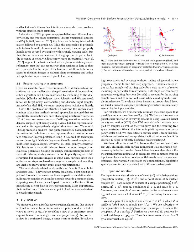
(a) Input (b) Crust (c) Refinement
Fig. 2. Data and method overview. (a) Ground truth geometry (black) and
input data consisting of samples (red) and (selected) views (blue). (b) Crust
(magenta) extraction based on occupancy scalar fieldwith varying resolution.
(c) Surface refinement to reduce the error (red) of the surface estimate.
high robustness and accuracy without trading off generality, we
propose a coarse-to-fine two-step approach. It handles noisy in-
put surface samples of varying scale for a vast variety of scenes
including, in particular thin structures. Both steps use compactly
supported weighting functions (kernels) to account for the varying
sample scales and to cancel out noise while avoiding undue sam-
ple interference. To evaluate these kernels at proper detail level,
we build a hierarchical space partitioning structure automatically
steered by the input samples.
For robustness, we first coarsely estimate the scene space that
possibly contains a surface, see Fig. 2(b). We find an intermediate
global scalar function with varying resolution using Bayesian kernel
density estimation (KDE). Our KDE models both the space occu-
pied by samples as well as their visibility and the resulting free
space constraints. We call this interim implicit representation occu-
pancy scalar field. We then extract a surface crust C from this field,
which overestimates and encapsulates the final output surface S. Inessence, C helps to robustly bootstrap reconstructing S.We then refine the crust C to become the final surface S, see
Fig. 2(c). This multi-scale surface refinement is a constrained non-
convex optimization problem. In each iteration, our algorithm shifts
the current surface estimate S to reduce its error computed from all
input samples using interpolation with kernels based on geodesic
distances. Importantly, S constrains the optimization by separating
spatially close kernels associated with different surface parts.
3.1 Input and notation
The input for our algorithm is a set of views vi with their positions(projection centers) piv ∈ R3 and a point cloud of N surface
samples s j . Each sample s j consists of a sample position pjs ∈ R3,
normal njs ∈ R3, optional confidence c js ∈ R and scale δ
js ∈ R.
Moreover, each sample s j was reconstructed for a reference view
vjref
and seen from a set of views V j ⊂ vi including the reference
view.
We call a pair of a sample s j and a view vi ∈ V j in which s j is
visible a linked view to sample pair (vi , s j ). We use subscripts to
mark quantities as belonging to a view v , a sample s , a node n, the
occupancy O or a surface S. Further, we denote all 3D positions by
a bold variable p, e.g., pjs , and 2D surface coordinates of a surface S
by a bold variable x, e.g., xi, j .
ACM Transactions on Graphics, Vol. 36, No. 6, Article 187. Publication date: November 2017.

187:4 • Aroudj, S. et al
Most passive and active reconstruction techniques can naturally
assign a view position to each view (e.g., the camera center capturing
an image or range scan). Confidences are optional, sample normals
and scales can be estimated in a preprocessing step [Fuhrmann et al.
2014]. We follow Fuhrmann et al. [2014] and define the scale (also
called 3D footprint) δjs of s
j as the average 3D distance of s j to its
neighboring samples in the reference viewvjref. We triangulate each
depth map, reproject it into 3D space and average the length of
incident 3D edges for each reprojected depth sample. Our surface
reconstruction method is therefore generally as applicable as most
related work, including [Curless and Levoy 1996; Jancosek and
Pajdla 2011; Labatut et al. 2009].
4 CRUST COMPUTATION
We first estimate two probability density functions (PDFs) within a
sparse voxel octree (SVO) using KDE. They represent space close to
surfaces inferred from samples and free space derived from visibility.
We then restrict the PDF for surface samples by the free space PDF,
yielding an occupancy scalar field from which we extract a coarse
crust C. This KDE-based crust extraction is very robust and yields, incontrast to previous work, a reliable encapsulation of thin structures
even in the presence of noise.
4.1 Sparse voxel octree
For definition of sample-driven and hence spatially varying recon-
struction level of detail as in Fuhrmann and Goesele [2014], we
insert all samples into a sparse voxel octree, see Fig. 2(b). Similar
to Ummenhofer and Brox [2015], each center pmn ∈ R3 of a leaf
node nm serves as an evaluation position at which we estimate an
implicit scene representation, the scalar occupancy field. A sample
s j is inserted into an octree node nm if nm contains the sample
position pjs and has a sufficiently small side length lmn ∈ R with
lmn ≤ hSVO · δ js < 2lmn . The user defined constant hSVO ∈ R controls
the overall scene sampling density. Since we evaluate the occupancy
field at leaf node centers, we need to ensure that there are leaf node
centers close enough in front of and behind the plane of a sample
patch s j . If necessary, we refine the SVO until we create evaluation
positions pmn within radius RjSVO
∈ R fulfilling a similar crite-
rion RjSVO
≤ hSVO · δ js on both sides of the sample patch plane.
We balance the tree to have a maximum depth difference of one
between directly neighboring leaf nodes as in Ummenhofer and
Brox [2015]. This yields a smoothly varying sampling grid for our
PDF estimations. Finally, we compute the dual of the SVO [Schaefer
and Warren 2004] for later crust surface extraction.
4.2 Probability Density Functions
One of the key aspects in kernel density estimation is the choice of a
suitable bandwidth for the kernels. It determines their spatial extend
and in turn their smoothing properties. There has been extensive
research in the machine learning community regarding this aspect.
An important approach is spatially varying the kernel bandwidth de-
pending on the kernel center or kernel evaluation position [Sheather
and Jones 1991]. Another method is selecting the bandwidth h to ful-
fill an optimality criterion, such as minimizing the expected L2 loss
pnm
D e
d sR r
p vi
p sj
nsj
ROj
ROj
ROj
ROj
R
r
de
pnm '
(a) Sample, kernel domains
d (psj)
D e
ROj
K depth(d , D)d ( pv
i )
d ( pnm)
de
d s
(b) kdepth
Fig. 3. Implicit scene representation via kernels. (a) Sample with position
pjs and normal n
js . Surface (red) and empty space (blue) kernel domains
consisting of discs parallel to the sample plane. The kernel parameters for an
evaluation position pmn are defined by the intersection (gray cross) of cone
axis and the disc through the node center pmn . (b) The 1D depth kernels.
between the unknown density f and its kernel density estimator f
(Variable KDE, [Terrell and Scott 1992]). In contrast, to represent
individual sample scales, multi-scale surface reconstruction tech-
niques typically vary the size of the corresponding basis functions
or they (less explicitly) define the per-sample scale via the depth
at which a sample is represented in a hierarchical data structure.
Motivated by this, we generalize this per-sample variation and not
only employ it for interpolation or sample splatting as in previous
work but also for KDE. In particular, we select the bandwidth of each
individual kernel based on the scale of the observation it represents.
Importantly, an observation is not only a mere surface sample since
sample scales also determine free space kernel bandwidths. We call
this observation-dependent KDE (ODKDE).
Our models for sample and empty space observations generally
build on a kernel radius Rj
O = hO · δ js at the samples’ locations for
KDE, which is proportional to the sample scale δjs and a user defined
smoothing factor hO (similar to Fuhrmann and Goesele [2014]). We
model both oblique circular cone kernel domains for free space
and for surfaces by sweeping circular discs with projected radius
R = proj(vi ,R jO) along the cone center axis. All such cone discs are
orthogonal to the respective sample normal njs , see Fig. 3(a).
We design the crust around the true surface as a Bayesian decision
boundary. C should conservatively enclose the true surface without
introducing topological artifacts such as wrongly filling gaps. Thus,
we define two corresponding classes: CE for empty space and CS
for space close to a surface. Note that CS does not represent the
space inside objects. We assign each leaf node center pmn to one of
these classes using the joint Bayesian probability densities
p(pmn ,CE ) = p(CE ) · p(pmn |CE ) (1)
p(pmn ,CS) = p(CS) · p(pmn |CS) (2)
and model our crust as decision boundary p(pmn ,CE ) = p(pmn ,CS).The class conditionals p(pmn |CE ) and p(pmn |CS) are PDFs calculatedusing ODKDE. The emptiness PDF models empty space between all
ACM Transactions on Graphics, Vol. 36, No. 6, Article 187. Publication date: November 2017.

Visibility-Consistent Thin Surface Reconstruction Using Multi-Scale Kernels • 187:5
linked pairs withM =(vi , s j )
:
p(pmn |CE ) = 1
M
∑
(v i ,s j )ki, je (pmn ) (3)
Each kernel ki, je : R3 7→ R maps a complete oblique circular view
cone to emptiness weights, see Fig. 3(a). The surfaceness PDF
p(pmn |CS) = 1
M
∑
(v i ,s j )ki, js (pmn ) (4)
represents the probability density of having surface samples within
the vicinity of leaf node centers. Each sample s j is similarly repre-
sented by a kernel ki, js : R3 7→ R within a cut oblique circular cone
centered at s j .
Each 3D kernel consists of a 2D kernel, kdisc, with a respective
projective circular disc as domain multiplied by a 1D kernel, kdepth,
with the corresponding cone axis as domain. More specifically, we
define them as
ki, je (pmn ) = kdisc (r ,R) · kdepth (de ,De ) (5)
ki, js (pmn ) = kdisc (r ,R) · 0.5 · kdepth
(|ds | ,R jO
)(6)
kdisc (r ,R) =
2
πR2
(1 − r 2
R2
)r < R
0 else(7)
kdepth (d,D) =
32D
(1 − d2
D2
)d < D
0 else.(8)
Fig. 3(a) shows the depths along a cone axis and the radial distance
r within a projected circular disc of radius R. For the sampleness ker-
nels ki, js , we use the same overall shape but within a more restricted
support volume. The cones for samples are cut at the beginning and
centered at the sample. Further, we reuse the 1D ray kernel kdepthfor samples but have kdepth centered at the samples, mirrored at the
sample plane and downscaled for∫ ∞−∞ 0.5 · kdepth (|ds |,Ds ) dds = 1,
see Fig. 3(b). The kernels ki, je and k
i, js are compactly supported,
non-negative and have a constant volume integral of one and are
thus suitable for PDF estimation.
The class priors p(CE ) and p(CS) represent a priori probabilitiesof leaf node centers belonging either to empty space or space near
surfaces. They express the generally higher probability of nodes to
belong to free space than to space close to a surface. For the priors
we first globally sum all cone main axis lengths per class to have
LE and LS . Then we estimate the priors via the total sums as
p(CE ) = LE
LE + LSp(CS) = LS
LE + LS. (9)
Note that we use axis lengths instead of cone volumes as they are
more robust for noisy sample normals.
When choosing the exact kernel functions, there are many de-
grees of freedom to account for different input data properties
and correspondingly many kernels are known and used [Adams
and Wicke 2009]. Generally, the kernel bandwidths (kernel support
ranges) are most crucial in KDE as the bandwidths define the trade-
off between overfitting and oversmoothing during PDF estimation.
ODKDE strongly alleviates the kernel bandwidth selection problem.
In contrast, the choice of the exact kernel shapes is less important.
In case of 3D surface reconstruction for which the number of linked
pairsM is usually high, different but proper PDF kernels result in
almost equal PDF estimates. Further, kernel parameters are partially
redundant. For example, flat kernels with small support range are
very similar to spiky kernels with large support range and therefore
result in very similar PDF estimates.
4.3 Crust extraction
We extract a surface crust C that serves as robust initial estimate
and constraint for the non-convex surface optimization detailed in
Sect. 5. C is not supposed to be an accurate reconstruction but should
be relatively close to the true surfaces, neither miss thin, small or
weakly-supported structures nor contain false geometry from outlier
clusters. Surfaces and empty space are mutually exclusive, so we
can combine the two estimated PDFs of Eqs. 3 and 4 into a single
implicit representation, our irregularly sampled occupancy scalar
field o(pmn ). For all leaf nodes we define occupancy as
o(pmn ) = p(pmn ,CS) − p(pmn ,CE ) (10)
with Bayesian decision boundary at isovalue zero. Further, we mark
leaf nodes with too sparse data as uncertain and avoid extracting
crust surfaces for them by setting o(pmn ) = −ϵ for all leaf nodes with∑
i, jki, je (pmn ) + ki, js (pmn ) < tC,k . The values of o(pmn ) are mainly
zero or negative in free space due to the view kernels. Further,
they rapidly increase close to the samples and towards the true
surfaces. Thus a moderate change of tC,k only noticeably influences
the extraction in sparsely sampled areas and defines how much of
weakly supported and thus often noisy crust is cut. Given scale-
dependent Gaussian noise on depth maps, Fig. 4 shows the crust for
the noisy wedge dataset from Fig. 1 with varying crust threshold
tC,k (top) and its robustness against increasing noise (bottom). Note
that C is truly a closed crust. It consists of an outer and inner side
at areas where objects are sufficiently thick.
Using the occupancy field o(pmn ), our algorithm extracts the
multi-scale crust C at the Bayesian decision boundary via dual
marching cubes [Schaefer and Warren 2004]. Importantly, C al-
ways overestimates the true surface and encapsulates it. The spatial
surface overestimation is proportional to the sample scales and
matches the sampling by the SVO. In particular, the crust overes-
timation is lower for fine details and higher for coarsely sampled
scene areas. Hence, we can still reconstruct holes in objects. More-
over, we circumvent the requirement of having leaf centers pmn within the exact thin structure by only requiring them to be within
C. We therefore do not have the aliasing problems of previous work
which explicitly represents filled space.
In addition, our algorithm deletes small isolated geometry compo-
nents caused by locally concentrated outlier sample clusters using
a triangle count threshold similar to Fuhrmann and Goesele [2014]
(isle size |nisle | < tC, isle). Further, the normals of the initial crust Care unreliable due to voxelization artifacts. We strongly smooth Cbefore the first refinement step using the Umbrella operator to have
better normals [Taubin 1995]. After that, the optimization starts
with the crust C as initial estimate S.
ACM Transactions on Graphics, Vol. 36, No. 6, Article 187. Publication date: November 2017.

187:6 • Aroudj, S. et al
(a) tC,k = 0.1 (b) tC,k = 50 (c) tC,k = 200 (d) tC,k = 400
(e) σ = 0.001 (f) σ = 0.01 (g) σ = 0.05 (h) σ = 0.1
Fig. 4. Crust extraction behavior for the synthetic wedge from Fig. 1. Noisy
input data created by ray tracing the synthetic wedge ground truth mesh
and adding depth noise with d = d +√d · N(0, σ ). Top: Varying the crust
threshold tC,k with constant σ = 0.1 noticeably influences the extraction
only in weakly sampled area as desired.Bottom: Increasing noise for constant
tC,k = 1 increases uncertainty of exact surface locations. Note that noise
results in crust expansion instead of the removal of thin surfaces.
5 SURFACE REFINEMENT
For a detailed final result, we iteratively evolve the initial surface
C to an accurate surface S. The functions pS : S 7→ R3 and nS :
S 7→ R3 map 2D surface coordinates x ∈ S to 3D coordinates and
normals. We define the error E of a given surface S with respect to
all input samples and their linked views
E(S,W) = 1
AS
∫
S
eS(x,W)dx (11)
as total reconstruction error normalized by the surface area AS via
the locally varying surface error function eS . Since our input con-sists of only point-based data, we need to robustly define the continu-
ous function eS for the whole surface. Thus, we interpolate samples
(or other quantities) over S using multi-scale kernels that define the
interpolation weighting functions W = wi, j
S : R2 7→ R. For eachlinked pair (vi , s j ), the weighting functionwi, j
S should spread over
the proper local area Ωi, j
S ⊂ S reconstructed for (vi , s j ), see Fig. 6.To implement that, we first intersect the ray from the view projection
center piv to the sample position pjs with S, yielding 2D coordinates
xi, j ∈ S of the projected sample (pi, j ,ni, j ) = (pS(xi, j ),nS(xi, j )).We then find geodesics (shortest paths on S) from xi, j to surround-
ing surface pointsΩi, j
S . Wemodify the geodesic distances to penalize
changes of surface normals from the respective sample s j and input
these modified distances into a standard normalized kernel with
implicit domain Ωi, j
S . Finally, we scale the entire kernel by two
confidences quantifying the quality of the matching of (vi , s j ) tothe surface S and the sample confidence itself to yield the required
weighting functionwi, j
S . Details are given in Sect. 5.1.
Importantly, our kernels spread only within S and not freely
within 3D space. Hence, a given surface S constrains our optimiza-
tion problem by restricting the kernels’ and thus samples’ influence
Noise-free
Noisyσ=0.05
(a) Crust (b) i = 1 (c) i = 3 (d) i = 10
Fig. 5. Surface refinement results. Note the increase in corner crispness and
strong initial error reduction, especially from (a) crust C to (b) S, i = 1.
to relevant nearby locations, which is why we call them data-driven
surface kernels. Note that we also define the kernel sizes via sample
scales enabling multi-scale surface interpolation and optimization.
The scene dependent constraints yield, however, a non-convex op-
timization problem since the surface estimate S depends on the
surface error E(S,W) and thus on the weights W. The weighting
functions W in turn depend on S. We linearize this problem by
iteratively refining S, using the crust C as robust starting point. In
each linearization step, we first completely fix S to calculate the
weighting functionsW. We then optimizeS while keepingW com-
pletely fixed. Sect. 5.2 details surface update steps using our novel
interpolation scheme and Fig. 5 shows an example optimization.
How to implement our optimization for a discrete triangle mesh
surface follows in Sect. 5.3.
5.1 Interpolation via surface kernels
Similar to previous methods [Curless and Levoy 1996; Fuhrmann
and Goesele 2014; Ummenhofer and Brox 2015], we approximate a
continuous function from samples via kernel-based interpolation.
For all linked pairs (vi , s j ), we interpolate point measurements
or surface functions f i, jS (x) of these via
fS(x,W) = 1
WS(x,W)∑
(v i ,s j )wi, j
S (x)f i, jS (x). (12)
over the fixed surface S instead of 3D functions in scene space.
WS : S 7→ R is the normalization function. W = wi, j
S (x) arecorresponding pair-based weighting functions:
WS(x,W) = ∑
(v i ,s j )wi, j
S (x), wi, j
S (x) = c jsNi, j
S ki, j
S (x). (13)
Eachwi, j
S consists of three components. For increased robustness,
we use the projection confidence N i, j
S ∈ R to weight down the
respective projection (pi, j ,ni, j ) onto S if it disagrees with s j (on
top of the standard input confidence cjs ). The kernel k
i, j
S computes
geodesic costs from xi, j to any x ∈ Ωi, j
S and maps the costs for x to
a normalized scalar as third component ofwi, j
S (x). Next, we detailN i, j
S and ki, j
S and describe the geodesic costs.
ACM Transactions on Graphics, Vol. 36, No. 6, Article 187. Publication date: November 2017.
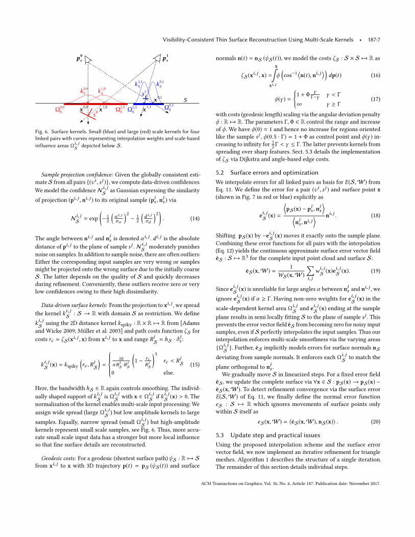
Visibility-Consistent Thin Surface Reconstruction Using Multi-Scale Kernels • 187:7
pv
0pv
1
S
x0,0
x1,0
x1,1
x0,1
kS
0,0kS
1,0kS
1,1kS
0,1
ΩS
0,0ΩS
1,0 ΩS
0,1
s0
s1
ΩS
1,1
Fig. 6. Surface kernels. Small (blue) and large (red) scale kernels for four
linked pairs with curves representing interpolation weights and scale-based
influence areas Ωi, j
S depicted below S.
Sample projection confidence: Given the globally consistent esti-
mateS from all pairs (vi , s j ), we compute data-driven confidences.
We model the confidenceN i, j
S as Gaussian expressing the similarity
of projection (pi, j ,ni, j ) to its original sample (pjs ,njs ) via
N i, j
S = exp
(− 12
(α i, j
σα
)2− 1
2
(d i, j
σd
)2). (14)
The angle between ni, j and njs is denoted α
i, j . di, j is the absolute
distance of pi, j to the plane of sample s j .N i, j
S moderately punishes
noise on samples. In addition to sample noise, there are often outliers:
Either the corresponding input samples are very wrong or samples
might be projected onto the wrong surface due to the initially coarse
S. The latter depends on the quality of S and quickly decreases
during refinement. Conveniently, these outliers receive zero or very
low confidences owing to their high dissimilarity.
Data-driven surface kernels: From the projection to xi, j , we spread
the kernel ki, j
S : S → R with domain S as restriction. We define
ki, j
S using the 2D distance kernel kspiky : R × R 7→ R from [Adams
and Wicke 2009; Müller et al. 2003] and path costs function ζS for
costs rc = ζS(xi, j , x) from xi, j to x and range Rj
S = hS · δ js :
ki, j
S (x) = kspiky(rc ,R
j
S
)=
10
πRj
S ·Rj
S
(1 − rc
Rj
S
)3rc < R
j
S
0 else.
(15)
Here, the bandwidth hS ∈ R again controls smoothing. The individ-
ually shaped support of ki, j
S is Ωi, j
S with x ∈ Ωi, j
S if ki, j
S (x) > 0. The
normalization of the kernel enables multi-scale input processing:We
assign wide spread (large Ωi, j
S ) but low amplitude kernels to large
samples. Equally, narrow spread (small Ωi, j
S ) but high-amplitude
kernels represent small scale samples, see Fig. 6. Thus, more accu-
rate small scale input data has a stronger but more local influence
so that fine surface details are reconstructed.
Geodesic costs: For a geodesic (shortest surface path)ψS : R 7→ Sfrom xi, j to x with 3D trajectory p(t) = pS (ψS(t)) and surface
normals n(t) = nS (ψS(t)), we model the costs ζS : S × S 7→ R as
ζS(xi, j , x) =x∫
xi, j
ϕ(cos−1
⟨n(t),ni, j
⟩)dp(t) (16)
ϕ(γ ) =1 + Φ
γΓ−γ γ < Γ
∞ γ ≥ Γ(17)
with costs (geodesic length) scaling via the angular deviation penalty
ϕ : R 7→ R. The parameters Γ,Φ ∈ R control the range and increase
of ϕ. We have ϕ(0) = 1 and hence no increase for regions oriented
like the sample s j , ϕ(0.5 · Γ) = 1 + Φ as control point and ϕ(γ ) in-creasing to infinity for 1
2 Γ < γ ≤ Γ. The latter prevents kernels from
spreading over sharp features. Sect. 5.3 details the implementation
of ζS via Dijkstra and angle-based edge costs.
5.2 Surface errors and optimization
We interpolate errors for all linked pairs as basis for E(S,W) fromEq. 11. We define the error for a pair (vi , s j ) and surface point x
(shown in Fig. 7 in red or blue) explicitly as
ei, j
S (x) =
⟨pS(x) − p
js ,n
js
⟩
⟨njs ,n
i, j⟩ ni, j . (18)
Shifting pS(x) by −ei, jS (x) moves it exactly onto the sample plane.
Combining these error functions for all pairs with the interpolation
(Eq. 12) yields the continuous approximate surface error vector field
eS : S 7→ R3 for the complete input point cloud and surface S:
eS(x,W) = 1
WS(x,W)∑
i, j
wi, j
S (x)ei, jS (x). (19)
Since ei, j
S (x) is unreliable for large angles α between njs and n
i, j , we
ignore ei, j
S (x) if α ≥ Γ. Having non-zero weights for ei, j
S (x) in the
scale-dependent kernel area Ωi, j
S and ei, j
S (x) ending at the sample
plane results in semi locally fitting S to the plane of sample s j . This
prevents the error vector field eS from becoming zero for noisy input
samples, even ifS perfectly interpolates the input samples. Thus our
interpolation enforces multi-scale smoothness via the varying areas
Ωi, j
S . Further, eS implicitly models errors for surface normals nSdeviating from sample normals. It enforces each Ω
i, j
S to match the
plane orthogonal to njs .
We gradually move S in linearized steps. For a fixed error field
eS , we update the complete surface via ∀x ∈ S : pS(x) → pS(x) −eS(x,W). To detect refinement convergence via the surface error
E(S,W) of Eq. 11, we finally define the normal error function
eS : S 7→ R which ignores movements of surface points only
within S itself as
eS(x,W) = ⟨eS(x,W),nS(x)⟩ . (20)
5.3 Update step and practical issues
Using the proposed interpolation scheme and the surface error
vector field, we now implement an iterative refinement for triangle
meshes. Algorithm 1 describes the structure of a single iteration.
The remainder of this section details individual steps.
ACM Transactions on Graphics, Vol. 36, No. 6, Article 187. Publication date: November 2017.
187:8 • Aroudj, S. et al
x
v0
v1
x0,1
k0,1k
1,0
e1,0(x1,0)
x ,
e0,1(x0,1)s
0
s1
e0,1(x)
(x1,0)
x1,0
e1,0(x )
n
e
Fig. 7. eS(x, W) (black). Point-based errors e0,1(x0,1) and e1,0(x1,0) fromray tracing (magenta). Interpolating the surface-dependent errors e0,1S (x)(blue) and e1,0S (x) (red) of the view sample pairs (v0
, s1) and (v1, s0) at x.
ALGORITHM 1: Each optimization step computes weights and inter-
polates sample quantities at each vertex x and robustly deforms S while
keeping a regular multi-scale triangle distribution.
1 collapse() // remove needle triangles from marching cubes or moves
2 ∀(v i , s j ): (pi, j , ni, j ) = traceRay(piv , pjs , S) // Embree [Wald et al. 2014]
3 ∀x: compute W,WS(x, W), eS(x, W), any fS(x, W) // Eqs. 12, 13, 194 ∀x: ifWS(x, W) < tS,weak : then markUnreliable(x)
5 foreach reliable x do
6 compute eS(x, W) // Eq. 207 if eS(x, W) > 2 · eS(x, W)old then8 pS(x) = pS(x)old, eS(x, W) = eS(x, W)old // revert9 else
10 pS(x) = pS(x) − eS(x, W) // advect11 end
12 end
13 if converged(E(S, W)) then return final S // Eq. 11
14 ∀x : pS(x) = umbrellaOp(x, λdist) // [Taubin 1995]
15 begin // handle outlier geometry
16 eraseUnreliableIsles() // if connected triangle count nisle < tS, isle17 patchHoles() // fill each hole ring with flat triangles
18 smoothIrregularIsles() // find and smooth badly moved vertices
19 end
20 split() // varying details: large triangles moved into small nodes?
21 ∀ unreliable x: pS(x) = umbrellaOp(x, λout) // the weak follow others
Kernel spread: We implemented the surface kernel ki, j
S using a
Dijkstra search over triangle edges starting at pi, j (Line 3). For each
potential step over an edge, we compute the angular deviation γ
between ni, j and the mean normal of the two triangles adjacent to
the edge. The penalty ϕ(γ ) (Eq. 17) then scales the edge length.
Surface support function: We useWS(x,W) (Eq. 13) as surfacesupport. It is low at weakly sampled areas such as scene borders
and occluded object regions.WS(x,W) is also zero for most hallu-
cinations at back sides that are not supported by samples but where
nevertheless a crust was extracted. We mark these areas via thresh-
olding with tS,weak (Line 4) which strongly facilitates removing
hallucinated geometry, see Fig. 13(j). In contrast to Fuhrmann and
Goesele [2014], ourWS(x,W) does not only increases with sample
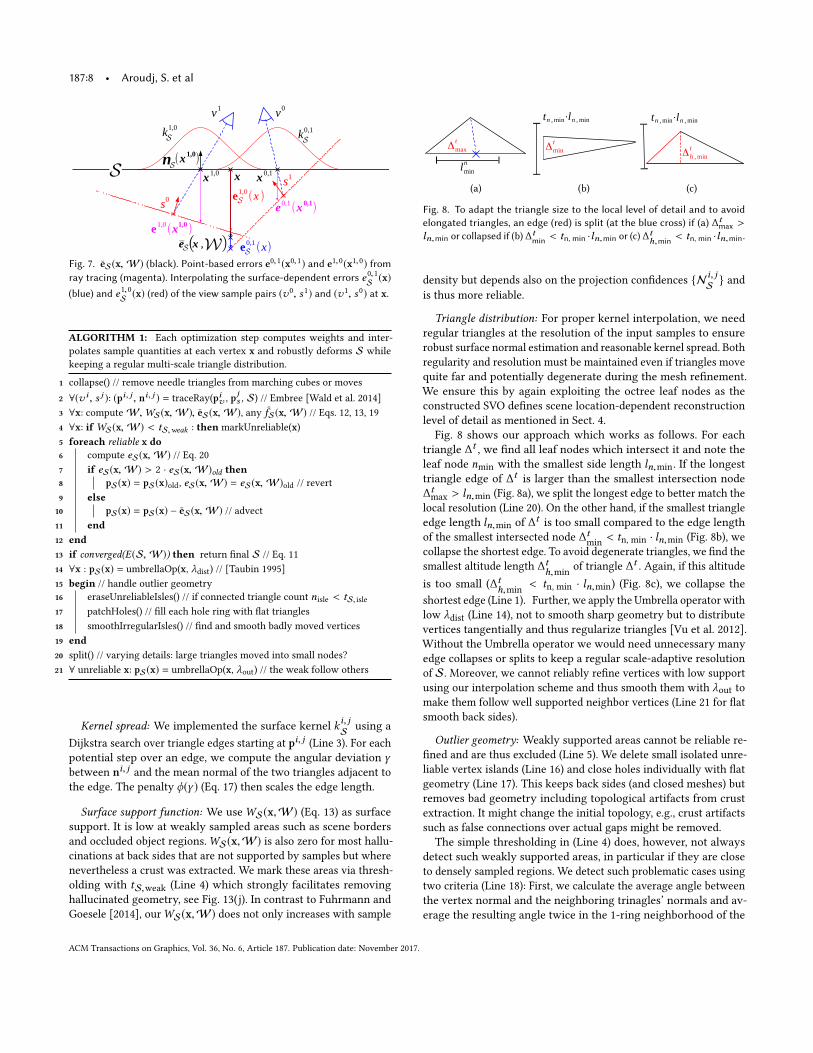
Δmax
t lmin
n(a)
Δmin
t
tn ,min⋅ln ,min
(b)
Δh ,min
t
tn ,min⋅ln ,min
(c)
Fig. 8. To adapt the triangle size to the local level of detail and to avoid
elongated triangles, an edge (red) is split (at the blue cross) if (a) ∆tmax >
ln,min or collapsed if (b) ∆tmin
< tn, min ·ln,min or (c) ∆th,min
< tn, min ·ln,min.
density but depends also on the projection confidences N i, j
S andis thus more reliable.
Triangle distribution: For proper kernel interpolation, we need
regular triangles at the resolution of the input samples to ensure
robust surface normal estimation and reasonable kernel spread. Both
regularity and resolution must be maintained even if triangles move
quite far and potentially degenerate during the mesh refinement.
We ensure this by again exploiting the octree leaf nodes as the
constructed SVO defines scene location-dependent reconstruction
level of detail as mentioned in Sect. 4.
Fig. 8 shows our approach which works as follows. For each
triangle ∆t , we find all leaf nodes which intersect it and note the
leaf node nmin with the smallest side length ln,min. If the longest
triangle edge of ∆t is larger than the smallest intersection node
∆tmax > ln,min (Fig. 8a), we split the longest edge to better match the
local resolution (Line 20). On the other hand, if the smallest triangle
edge length ln,min of ∆t is too small compared to the edge length
of the smallest intersected node ∆tmin< tn, min · ln,min (Fig. 8b), we
collapse the shortest edge. To avoid degenerate triangles, we find the
smallest altitude length ∆th,min
of triangle ∆t . Again, if this altitude
is too small (∆th,min
< tn, min · ln,min) (Fig. 8c), we collapse the
shortest edge (Line 1). Further, we apply the Umbrella operator with
low λdist (Line 14), not to smooth sharp geometry but to distribute
vertices tangentially and thus regularize triangles [Vu et al. 2012].
Without the Umbrella operator we would need unnecessary many
edge collapses or splits to keep a regular scale-adaptive resolution
of S. Moreover, we cannot reliably refine vertices with low support
using our interpolation scheme and thus smooth them with λout to
make them follow well supported neighbor vertices (Line 21 for flat
smooth back sides).
Outlier geometry: Weakly supported areas cannot be reliable re-
fined and are thus excluded (Line 5). We delete small isolated unre-
liable vertex islands (Line 16) and close holes individually with flat
geometry (Line 17). This keeps back sides (and closed meshes) but
removes bad geometry including topological artifacts from crust
extraction. It might change the initial topology, e.g., crust artifacts
such as false connections over actual gaps might be removed.
The simple thresholding in (Line 4) does, however, not always
detect such weakly supported areas, in particular if they are close
to densely sampled regions. We detect such problematic cases using
two criteria (Line 18): First, we calculate the average angle between
the vertex normal and the neighboring trinagles’ normals and av-
erage the resulting angle twice in the 1-ring neighborhood of the
ACM Transactions on Graphics, Vol. 36, No. 6, Article 187. Publication date: November 2017.

Visibility-Consistent Thin Surface Reconstruction Using Multi-Scale Kernels • 187:9
vertex in order to increase robustness. If the smoothed angle is
larger than the threshold angle tβ we regard the corresponding
vertex as a spiky outlier. Second, we also mark vertices as spiky
outliers if their average incident edge length, i.e., their scale is more
than doubled after updating the positions of the reliable vertices in
Lines 5ś12. Note that triangle sizes and thus edge lengths should
mainly decrease during refinement: Triangles are subdivided if they
are moved into smaller SVO nodes (Line 20) but are typically not
moved into larger nodes or coarser sampled scene space. To robustly
handle such spiky outlier vertices, which only occur as small islands,
we fit them to their well-refined neighbors by smoothing them until
convergence using the Umbrella operator.
6 RESULTS
We compare TSR against Poisson Surface Reconstruction (PSR)
[Kazhdan and Hoppe 2013], Floating Scale Surface Reconstruction
(FSSR) [Fuhrmann andGoesele 2014], Ummenhofer and Brox’s point-
based reconstruction (UPoi) [2013], Point Fusion (PFS) [Ummen-
hofer and Brox 2015], Smooth Signed Distance Surface Reconstruc-
tion (SSD) [Calakli and Taubin 2011], Surface Reconstruction from
Multi-resolution Points (SURFMRS) [Mücke et al. 2011] and CMP-
MVS [Jancosek and Pajdla 2011] using the original implementations
of the authors except for CMPMVS* in Fig. 1 where we needed to
use our own implementation. Note that we never cull back faces.
Additionally, back faces of colorless reconstructions are rendered in
yellow. TSR performance is in Tab. 1 with peak memory consump-
tion measured as the maximum resident memory size of the process.
Tab. 2 lists the parameter values for the presented scenes.
Synthetic tests and benchmark: Fig. 1 shows the synthetic wedge,
a thin structure with optional Gaussian noise in the bottom rows
(σ = 0.1). We generated only one reference view and no addi-
tional views per synthetic surface sample. Our qualitative evaluation
shows that while related work already cannot accurately reconstruct
the wedge given perfect samples, our approach is able to faithfully
reconstruct the wedge even in the presence of noise. The visual-
ized error shows that front and back of the wedge do not interfere
with each other. Tab. 3 quantitatively details the bottom row re-
sults. To avoid punishing artifacts at the open boundary due to the
finite size of the synthetic ground truth wedge, we evaluated only
reconstructed surfaces within the gray box depicted in Fig. 1(a).
TSR always performs best. Note that the Middlebury evaluation
methodology does not consider surface orientations and may match
the reconstructed front with the ground truth back (and vice versa).
This falsely increases completeness values for all other methods for
areas where they accurately reconstructed only one but not both
sides of the thin structure.
Fig. 9 presents a large city model. We created a version textured
with simplex noise, simulated 287 photographs, and fed these into
MVE [Fuhrmann et al. 2014] for multi-view stereo-based point cloud
reconstruction. Fig. 9 demonstrates that all other approaches have
issues with correctly reconstructing the edges and planar surfaces.
In particular, the thin roof railings highlighted in Fig. 9(a) are either
missing (SSD, SURFMRS), incomplete (FSSR, CMPMVS) or show
significant errors due to front-back interference (FSSR, PFS, PSR).
(a) Ground truth (b) FSSR (c) PFS (d) SSD
(e) CMPMVS (f) SURFMRS (g) PSR (h) TSR
-10 10
Accuracy (errors) Completeness (%)
95% 90% 80% 9.50 5.00 2.50
SSD 14.04 10.33 6.68 70.9 59.0 44.3
SURFMRS 7.20 5.32 3.70 87.9 78.9 55.7
CMPMVS 7.96 4.11 2.60 95.3 90.6 78.9
PSR 3.19 1.67 0.76 99.0 97.5 93.6
PFS 3.82 1.20 0.55 98.9 97.2 93.9
FSSR 3.40 1.12 0.46 98.0 94.9 91.4
TSR 1.22 0.61 0.33 99.0 98.4 96.4
(i) Accuracy and completeness according to the Middlebury Mview
evaluation methodology [Seitz et al. 2006]
Method Face count Runtime Peak memory
PFS 24, 416, 218 1h 13m 17GB
FSSR 19, 134, 127 1h 18m 27GB
TSR 71, 532, 306 18h 30m 79GB
(j) Performance (result size, total runtime and peak memory)
Fig. 9. City dataset. (a - h) Closeups visualizing thin roof railings highlighted
in (a). Note lower accuracy and missing or overestimated thin structures
for previous work. (i) TSR clearly dominates the quantitative evaluation. (j)
TSR, however, has highest runtime and memory demand.
(a) Image (b) Depths (c) Points, views (d) TSR
Fig. 10. Consumer depth sensor test. (a - b) Example input frame. (c) TSR
input: 1000 Kinect views (frames) [Sturm et al. 2012]. (d) Reconstruction.
TSR keeps not only these structures but also consistently performs
best in the quantitative evaluation, see Fig. 9(i).
As a sanity check, we submitted our results for the full temple
to the Middlebury multi-view stereo evaluation [Seitz et al. 2006]
and achieved state of the art results (accuracy: 0.36mm for 90%,
completeness: 99.2 % within 1.25mm).
ACM Transactions on Graphics, Vol. 36, No. 6, Article 187. Publication date: November 2017.

187:10 • Aroudj, S. et al
Sample count Face count Peak memory Total time SVO Occupancy Refinement
City 361, 058, 245 71, 532, 306 79GB 18h 30m 1h 20m 2h 16m 14h 54m
Citywall 292, 415, 380 52, 379, 087 67GB 17h 22m 1h 2m 7h 21m 8h 59m
Cardboard 76, 540, 423 17, 372, 889 38GB 16h 33m 23m 2h 17m 13h 53m
Orchid 16, 237, 665 8, 429, 311 26GB 4h 7m 6m 1h 28m 2h 33m
Temple 15, 568, 210 1, 055, 670 20GB 44m 3m 15m 26m
ShellTower 7, 942, 563 1, 720, 804 20GB 24m 1m 8m 14m
Table 1. Point cloud sizes, face counts of results, peak memory consumption and runtimes for TSR. Total time from input loading to final mesh output. SVO,
occupancy and refinement refer to the time from input loading to SVO output, time for occupancy scalar field computation and complete surface refinement
for a server with two Intel E5-2650V2 processors.
hSVO hO hSWedge 0.25 1 1
(noisy) 5 3 1
City 1 1 1
Citywall 2.5 3 1
Cardboard 1 1.5 1
Orchid 1 3 2
Temple 1 1.5 0.75
ShellTower 1 1.5 1
Teddy 1 1 1
σα π/9σd 2R
j
S/3Γ 5π/12Φ 0.1
tC,k 100
tC, isle 2500
tn, min 0.1
tS,weak 1.0
tS, isle 100
tβ π/6λdist 0.1
λout 1.0
Table 2. TSR parameters. hSVO, hO , hS control the smoothing strength
according to input data accuracy.
Accuracy (errors) Completeness (%)
95% 90% 80% 2 1 0.5
PSR 1.43 9.78 2.79 88.9 68.9 46.2
PFS 3.48 2.73 2.00 81.8 54.4 29.6
SSD 4.59 2.60 1.76 64.4 34.1 16.4
FSSR 3.47 2.28 1.51 83.9 65.7 40.5
CMPMVS 3.11 1.97 1.39 61.0 52.3 35.9
TSR 1.18 0.98 0.76 94.8 87.9 62.8
Table 3. Synthetic wedge (σ = 0.1) reconstruction accuracy and complete-
ness comparison (Middlebury Mview methodology [Seitz et al. 2006]).
General scenes: We show the generality of TSR by testing it on
the TUM RGB-D fr3 teddy scene [Sturm et al. 2012], see Fig. 10. TSR
reconstructs fine details such as the creases in the teddy’s shirt (Fig.
10(d)) despite the quantized Kinect depth maps (Fig. 10(b)).
We reconstructed the CityWall scene of Fig. 11 provided with
MVE for demonstration of multi-scale support. The uncontrolled
data set consists of 564 images captured with strongly varying
distances to the surfaces. CMPMVS is clearly inferior to the other
approaches as it fails to correctly model the varying scale of the
input samples. It oversmoothes the lion head and misses the thin
metal bars, see Fig. 11(b). FSSR, PFS and TSR produce highly detailed
geometry for the text on the wall and the lion heads. These areas
are particularly challenging as they contain overlapping samples
with strongly varying scale.
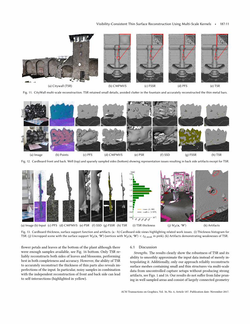
Thin structures: Fig. 12 shows a real 1mm thick piece of cardboard
with printed noise texture and additionally attached markers. We
captured 178 photographs for point cloud reconstruction with MVE.
The figures show the estimated geometry cropped to the approxi-
mate bounding box of the cardboard. PFS, FSSR and TSR reconstruct
the well sampled front side well while only TSR is able to also recon-
struct the sparser sampled back. The reconstructions of CMPMVS,
SSD and FSSR miss much cardboard surface area. PFS, PSR and SSD
hallucinate large amounts of geometry. In addition, our approach is
the only one correctly capturing the cardboard thickness, see Fig. 13.
We computed the histogram by rendering the distance (depth) from
the camera to the front and back side of the TSR reconstruction and
subtracted the resulting depth maps to get the thickness at every
pixel. The histogram consists of the accumulated pixel difference
values excluding areas of the attached markers. The mean of the
difference values is 1,2mm and hence close to the true thickness.
Fig. 13(j) additionally presents the closed surface S before cropping
weakly supported vertices and the corresponding support function
WS(x,W) of Eq. 13. Fig. 13(k) highlights TSR weaknesses: topo-
logical artifacts left from crust extraction, refinement convergence
to wrong local minima, and self-intersections due to noisy input
samples, see also Sec. 6.1.
A further challenging scene for thin structures is the Streetsign
from Ummenhofer and Brox [2013] with only one reference view
per sample, see Fig. 14. Their point cloud processing techniques
produce less noise in the front view. When observing the side view,
we notice, however, that the sign is a single plane, basically flattening
the entire geometry of the frame instead of actually reconstructing
it. In contrast, TSR does not oversmooth the geometry, reconstructs
the metal pillars and frame better but suffers from the many input
samples clustered before or behind the street sign leading to an
overestimation of the surface.
The next test scene is a point cloud of a miniature tower and a
small sea shell, see Fig. 15. For this challenging scene, our approach
is the only one that is able to produce a reconstruction containing
only a few holes while avoiding hallucinated geometry. FSSR and
PFS simplymiss one of the sea shell sides while PSR and SSD produce
hallucinated geometry. CMPMVS fares second best but again misses
geometry for very thin structures.
Our final test scene is the point cloud of an orchid reconstructed
with MVE. The reconstruction is challenging due to the thin struc-
tures as well as the amount of noise contained. Fig. 16 shows that
PSR, FSSR, and SSD produce large quantities of spurious geometry
while PFS and SSD miss thin or fine structures. Even though CMP-
MVS produces a substantially better result, it overestimate thickness
of leaves and blossom petals. CMPMVS also misses geometry for
ACM Transactions on Graphics, Vol. 36, No. 6, Article 187. Publication date: November 2017.
Visibility-Consistent Thin Surface Reconstruction Using Multi-Scale Kernels • 187:11
(a) Citywall (TSR) (b) CMPMVS (c) FSSR (d) PFS (e) TSR
Fig. 11. CityWall multi-scale reconstruction. TSR retained small details, avoided clutter in the fountain and accurately reconstructed the thin metal bars.
Front
Back
(a) Image (b) Points (c) PFS (d) CMPMVS (e) PSR (f) SSD (g) FSSR (h) TSR
Fig. 12. Cardboard front and back. Well (top) and sparsely sampled sides (bottom) showing representation issues resulting in back side artifacts except for TSR.
(a) Image (b) Input (c) PFS (d) CMPMVS (e) PSR (f) SSD (g) FSSR (h) TSR (i) TSR thickness (j)WS(x, W) (k) Artifacts
Fig. 13. Cardboard thickness, surface support function and artifacts. (a - h) Cardboard side views highlighting related work issues. (i) Thickness histogram for
TSR. (j) Uncropped scene with the surface supportWS(x, W) (vertices withWS(x, W) < tS,weak in pink). (k) Artifacts demonstrating weaknesses of TSR.
flower petals and leaves at the bottom of the plant although there
were enough samples available, see Fig. 16 bottom. Only TSR re-
liably reconstructs both sides of leaves and blossoms, performing
best in both completeness and accuracy. However, the ability of TSR
to accurately reconstruct the thickness of thin parts also reveals im-
perfections of the input. In particular, noisy samples in combination
with the independent reconstruction of front and back side can lead
to self-intersections (highlighted in yellow).
6.1 Discussion
Strengths. The results clearly show the robustness of TSR and its
ability to smoothly approximate the input data instead of merely in-
terpolating it. Additionally, only our approach reliably reconstructs
surface meshes containing small and thin structures via multi-scale
data from uncontrolled capture setups without producing strong
artifacts, see Figs. 1 and 16. Our results do not suffer from false prun-
ing in well sampled areas and consist of largely connected geometry
ACM Transactions on Graphics, Vol. 36, No. 6, Article 187. Publication date: November 2017.

187:12 • Aroudj, S. et al
(a) Image (b) Side (c) UPoi (d) TSR C (e) TSR S
(f) Front (g) UPoi (h) TSR C (i) TSR S
Fig. 14. Street sign comparison with UPoi. The sign reconstructed by both
TSR (noisy) and UPoi (oversmooth) despite strongly inaccurate samples.
(a) Image (b) Points (c) FSSR (d) PFS
(e) PSR (f) SSD (g) CMPMVS (h) TSR
Fig. 15. Shelltower comparison. Like for the cardboard, only TSR accurately
reconstructs the thin structures of the scene.
with floating parts only in areas with substantially missing data. On
top of that, the crust C is always extracted as closed mesh and kept
watertight during refinement. Still, we can identify and delete all
hallucinated fill-in and back side geometry via the surface support
functionWS(x,W), see Fig. 13(j). The iterative projective surfacecorrections implicitly define gradient descent step sizes depending
on surface error magnitudes. Thus, the refinement converges for
most surface parts after a few iterations, especially in well sam-
pled areas, see Fig. 5. Finally, we only employ local optimization
operations so that our algorithm scales well.
Weaknesses. The extracted crust C can have deficiencies. It might
wrongly reach over gaps or falsely connect surfaces if respective
visibility constraints are insufficient, see Fig. 13(k). This problem
is scale dependent (like the crust) and finer sampling alleviates it.
These artifacts can hamper the following surface evolution since
the initial solution is locally too far from the surface.
The refinement has weaknesses inherent to gradient descent: slow
convergence for fast changing gradients (e.g., due to contradicting
samples), convergence to local optima (possible for concavities, clus-
tered outliers, etc; see Figs. 1 and 13(k)) and no convergence guar-
antee owing to the non-convexity. In a few cases, triangle updates
for error reduction create false creases, hampering convergence due
to the angular costs function of our surface kernels. These disad-
vantages are the main source of missing details compared to related
work and might be reduced by an added smoothness energy term.
Accurately reconstructing the boundaries of thin structures is
difficult. There are usually no samples of the thin structure edges
(e.g., leaf edges) bounding the extend of the structures. The input
samples though require inter- and extrapolation which is thus not
precisely defined at the boundaries. Further, the Umbrella operator
leads to surface shrinkage at the same areas which is not reverted
by surface update steps due to the lack of respective samples.
Finally, the current implementation has the highest runtime and
memory usage of all competing approaches, see Fig. 9(j), leaving
room for further algorithmic improvement and code optimization.
7 CONCLUSION
Despite decades of research on surface reconstruction, many mod-
ern techniques are still not able to reliably reconstruct a simple
sheet of cardboard. We addressed in this paper the fundamental
underlying deficiencies of models and representations preventing
the reconstruction of thin surfaces. This allows TSR to faithfully
reconstruct scenes with thin surface parts as well as more traditional
single- and multi-scale scenes.
Besides improvements to the efficiency of the implementation
we see different directions for future work. First, we would like
to consistently address intersections of front and back side of thin
surfaces reconstructed from noisy data without introducing a bias
that increases the thickness of surfaces. Second, we plan to inte-
grate photometric consistency into our approach by taking not only
oriented point sets but also images of the scene as input for the
reconstruction. Image edges might also help to better reconstruct
thin and small structure borders. Third, to cope with scene-varying
sample noise strength, automatic selection of the resolution and
bandwidth parameters hSVO, hO and hS is necessary. Finally, our
approach is limited to static scenes. To remove this limitation and
enable a larger scene variety, especially uncontrolled reconstruction
of real plants, we will investigate modeling of object deformations.
ACKNOWLEDGMENTS
Part of this work was funded by the European Community’s FP7
programme under grant agreement ICT-323567 (Harvest4D). We
thank the FalconViz CAD team and Nils Moehrle for the City dataset.
REFERENCESBart Adams and Martin Wicke. 2009. Meshless Approximation Methods and Applica-
tions in Physics Based Modeling and Animation.. In Eurographics (Tutorials).Fausto Bernardini, Joshua Mittleman, Holly Rushmeier, Cláudio Silva, and Gabriel
Taubin. 1999. The Ball-Pivoting Algorithm for Surface Reconstruction. IEEE TVCG5, 4 (1999).
Fatih Calakli and Gabriel Taubin. 2011. SSD: Smooth Signed Distance Surface Recon-struction. CGF 30, 7 (2011).
Fatih Calakli and Gabriel Taubin. 2012. SSD-C: Smooth Signed Distance Colored SurfaceReconstruction. In Expanding the Frontiers of Visual Analytics and Visualization.
Yang Chen and Gérard Medioni. 1995. Description of complex objects from multiplerange images using an inflating balloon model. CVIU 61, 3 (1995).
ACM Transactions on Graphics, Vol. 36, No. 6, Article 187. Publication date: November 2017.

Visibility-Consistent Thin Surface Reconstruction Using Multi-Scale Kernels • 187:13
(a) Image (b) Points (c) PFS (d) PSR (e) SSD (f) FSSR (g) CMPMVS (h) TSR
Fig. 16. Comparison using the challenging orchid dataset. Most accurate and complete reconstruction by TSR. Other approaches with false pruning or
thickening and hallucinated geometry.
Brian Curless and Marc Levoy. 1996. A Volumetric Method for Building ComplexModels from Range Images. In SIGGRAPH.
Brian Lee Curless. 1997. New methods for Surface Reconstruction from Range Images.Dissertation. Stanford University.
Julie Digne, Jean-Michel Morel, Charyar-Mehdi Souzani, and Claire Lartigue. 2011.Scale space meshing of raw data point sets. In CGF, Vol. 30.
Simon Fuhrmann and Michael Goesele. 2011. Fusion of Depth Maps with MultipleScales. ACM TOG 30, 6 (2011).
Simon Fuhrmann and Michael Goesele. 2014. Floating Scale Surface Reconstruction.ACM TOG 33, 4 (2014).
Simon Fuhrmann, Fabian Langguth, and Michael Goesele. 2014. MVE - A Multi-ViewReconstruction Environment. In GCH, Vol. 6.
Hugues Hoppe, Tony DeRose, Tom Duchamp, John McDonald, and Werner Stuetzle.1992. Surface Reconstruction from Unorganized Points. In SIGGRAPH.
Alexander Hornung and Leif Kobbelt. 2006. Robust Reconstruction of Watertight 3DModels from Non-uniformly Sampled Point Clouds Without Normal Information.In SGP.
Michal Jancosek and Tomás Pajdla. 2011. Multi-View Reconstruction PreservingWeakly-Supported Surfaces. In CVPR.
Michael Kass, Andrew Witkin, and Demetri Terzopoulos. 1988. Snakes: Active contourmodels. IJCV 1, 4 (1988).
Michael Kazhdan and Hugues Hoppe. 2013. Screened Poisson Surface Reconstruction.ACM TOG 32, 3 (2013).
Patrick Labatut, Jean-Philippe Pons, and Renaud Keriven. 2009. Robust and EfficientSurface Reconstruction from Range Data. In CGF, Vol. 28.
Paul Merrell, Amir Akbarzadeh, Liang Wang, Philippos Mordohai, Jan-Michael Frahm,Ruigang Yang, David Nistér, and Marc Pollefeys. 2007. Real-Time Visibility-BasedFusion of Depth Maps. In ICCV.
Patrick Mücke, Ronny Klowsky, and Michael Goesele. 2011. Surface Reconstructionfrom Multi-resolution Sample Points. In VMV.
Matthias Müller, David Charypar, and Markus Gross. 2003. Particle-based Fluid Simu-lation for Interactive Applications. In SCA.
Richard A. Newcombe, Shahram Izadi, Otmar Hilliges, David Molyneaux, David Kim,Andrew J. Davison, Pushmeet Kohli, Jamie Shotton, Steve Hodges, and AndrewFitzgibbon. 2011. KinectFusion: Real-time Dense Surface Mapping and Tracking. InInternational Symposium on Mixed and Augmented Reality (ISMAR).
Yutaka Ohtake and Alexander G Belyaev. 2003. Dual-Primal Mesh Optimization forPolygonized Implicit Surfaces With Sharp Features. Journal of Computing andInformation Science in Engineering 2, 4.
Nikolay Savinov, Christian Häne, L’ubor Ladický, and Marc Pollefeys. 2016. Semantic3D Reconstruction with Continuous Regularization and Ray Potentials Using a
Visibility Consistency Constraint. In CVPR.Scott Schaefer and Joe Warren. 2004. Dual Marching Cubes: Primal Contouring of Dual
Grids. In PG.Steven M. Seitz, Brian Curless, James Diebel, Daniel Scharstein, and Richard Szeliski.
2006. A Comparison and Evaluation of Multi-View Stereo Reconstruction Algo-rithms. In CVPR, Vol. 1.
Qi Shan, Brian Curless, Yasutaka Furukawa, Carlos Hernandez, and Steven Seitz. 2014.Occluding Contours for Multi-View Stereo. In CVPR.
Simon J Sheather and Michael Chris Jones. 1991. A reliable data-based bandwidthselection method for kernel density estimation. Journal of the Royal StatisticalSociety. Series B (Methodological).
J. Sturm, N. Engelhard, F. Endres, W. Burgard, and D. Cremers. 2012. A Benchmark forthe Evaluation of RGB-D SLAM Systems. In IROS.
Gabriel Taubin. 1995. A Signal Processing Approach to Fair Surface Design. In SIG-GRAPH.
George R. Terrell and David W. Scott. 1992. Variable Kernel Density Estimation. TheAnnals of Statistics 20, 3 (1992).
Greg Turk and Marc Levoy. 1994. Zippered Polygon Meshes from Range Images. InSIGGRAPH.
Benjamin Ummenhofer and Thomas Brox. 2013. Point-Based 3D reconstruction of thinobjects. In ICCV.
Benjamin Ummenhofer and Thomas Brox. 2015. Global, Dense Multiscale Reconstruc-tion for a Billion Points. In ICCV.
Hoang-Hiep Vu, Patrick Labatut, Jean-Philippe Pons, and Renaud Keriven. 2012. HighAccuracy and Visibility-Consistent Dense Multiview Stereo. TPAMI 34, 5 (2012).
Ingo Wald, Sven Woop, Carsten Benthin, Gregory S. Johnson, and Manfred Ernst. 2014.Embree: A Kernel Framework for Efficient CPU Ray Tracing. ACM TOG 33, 4, Article143.
Kaan Yücer, Changil Kim, Alexander Sorkine-Hornung, and Olga Sorkine-Hornung.2016a. Depth from Gradients in Dense Light Fields for Object Reconstruction. In3DV.
Kaan Yücer, Alexander Sorkine-Hornung, Oliver Wang, and Olga Sorkine-Hornung.2016b. Efficient 3D Object Segmentation from Densely Sampled Light Fields withApplications to 3D Reconstruction. ACM TOG 35, 3 (2016).
Received May 2017; revised August 2017; final version September 2017;
accepted September 2017
ACM Transactions on Graphics, Vol. 36, No. 6, Article 187. Publication date: November 2017.