Embed Size (px)
Citation preview

Vision-based Indoor Navigation of a Semi-autonomous and Interactive
Unmanned Aerial System
Undergraduate Thesis
Presented in Partial Fulfillment of the Requirements for the Bachelor of Science with Research
Distinction in the Undergraduate School of The Ohio State University
By
Hongyun Elliot Lee
Undergraduate Program in Aeronautical and Astronautical Engineering
The Ohio State University
Department of Mechanical and Aerospace Engineering
April 2017
Thesis Committee:
Dr. Matthew McCrink, Adviser
Dr. Clifford A. Whitfield

Copyright by
Hongyun Lee
2017

ii
Abstract
This paper considers the development and implementation of a vision-based onboard flight
management computer (FMC) and inertial navigation system (INS) that can estimate and control
the attitude and relative position of the vehicle while interacting with an operator in an indoor
environment. In this project, a hexacopter is developed which uses an onboard inertial
measurement unit (IMU), a small-sized computer, and a Microsoft Kinect sensor. Since
directional maneuver of the hexacopter can be achieved by changing the angular position of the
vehicle, the project consists of inertial and vision sensor fusion.
To accomplish stable control of the multicopter's orientation, a complementary filter is
implemented on the IMU. Since the raw sensors do not provide an accurate angular position of
the vehicle per se, the complementary filter is used to fuse the raw sensor data to provide low-
noise and low-drift estimation of Euler angles. Autonomous indoor flight requires position
sensors other than GPS whose accuracy is approximately 2 to 3 meters. GPS signals are typically
unavailable in an indoor environment. In this project, a computer vision algorithm is used to
provide position estimation. The vision algorithm uses an onboard Microsoft Kinect and a
computer to execute EmguCV and Kinect SDK libraries. Since Kinect can provide color and depth
data, it allows to detect an object and to provide its real-time local coordinates which can be
used for an autonomous indoor flight. The coordinates are used to correct the position of the
vehicle. Also, to input commands such as takeoff, landing, proceed, retreat during the flight, an

iii
artificial neural network is used to classify human gestures so that the gesture can be used as
the commands.
The system is expected to maintain vehicle position within 1 meter for the better accuracy when
compared to low-cost GPS receivers, and to control corresponding angular orientation for the
position control. Also, the system is expected to interact with an operator within a reasonable
interaction while it can maintain the given flight control tasks.

iv
Dedication
I dedicate this paper to my family.

v
Acknowledgements
My work would have been impossible without my advisers. I would like to express my gratitude
to them. Dr. Whitfield offered me a lab space to work on and supported my idea and advised
the directions for the project from the very beginning to the end. I also learned a lot form Dr.
McCrink about knowledge and concepts. He always supported me when I was having difficult
time to understand them. My struggles became a part of this work and that was possible
because of my advisers' guidance. Again, I sincerely appreciate their efforts.
I also appreciate my family who supported my education abroad in the U.S. It must be difficult
decision to my parents, especially, due to the fiscal aspect. Finally, to all my friends who
provided their supports and feedbacks, thank you.

vi
Table of Contents
Abstract ..................................................................................................................... ii
Dedication ................................................................................................................. iv
Acknowledgements .................................................................................................... v
List of Tables ............................................................................................................ viii
List of Figures ............................................................................................................ ix
Chapter 1. Introduction .............................................................................................. 1
1.1 Overview ......................................................................................................................1
1.2 Objective ......................................................................................................................2
Chapter 2. System Overview ....................................................................................... 4
2.1 Hardware .....................................................................................................................4 2.1.1. Vehicle Frame and Power System ................................................................................................ 5 2.1.2 Sensors ........................................................................................................................................... 7 2.1.3 Onboard Computers ...................................................................................................................... 9 2.1.4 Battery ......................................................................................................................................... 10 2.1.5 XBee ............................................................................................................................................. 11 2.1.6 DC to DC Buck Converter ............................................................................................................. 12 2.1.7 Voltage Divider-Follower Circuit .................................................................................................. 12 2.1.8 Supplementary Circuits ................................................................................................................ 13
2.2 Software .................................................................................................................... 15 2.2.1 Onboard Computers .................................................................................................................... 16
2.3 Ground Control Station and Laboratory Environment .................................................. 16 2.3.1 Ground Control Station................................................................................................................ 16 2.3.2 Laboratory Environment .............................................................................................................. 17
Chapter 3. Inertial Measurement Unit....................................................................... 19
3.1 Overview .................................................................................................................... 19
3.2 Coordinate Systems and Rotation Matrix .................................................................... 19
3.3 Inertial Sensors ........................................................................................................... 22 3.3.1 Gyroscope and Accelerometer .................................................................................................... 22 3.3.2 Magnetometer............................................................................................................................. 23
3.4 Complementary Filter ................................................................................................. 25 3.4.1 Rotation Matrix Construction ...................................................................................................... 26 3.4.2 Error Correction ........................................................................................................................... 27

vii
3.5 Results ....................................................................................................................... 30 3.5.1 Simulation Result ......................................................................................................................... 30 3.5.2 Implementation ........................................................................................................................... 31 3.5.3 Experimental Result ..................................................................................................................... 34
Chapter 4. Vision Sensor and Flight Management Computer ..................................... 36
4.1 Color Tracking ............................................................................................................. 36 4.1.1 Color Space Conversion ............................................................................................................... 37 4.1.2 Thresholding ................................................................................................................................ 39 4.1.3 Morphological Operation ............................................................................................................ 40
4.1.4 Contour and Relative Coordinate Estimation .......................................................................... 41
4.2 Body Part Detection .................................................................................................... 45
4.3 Human Robot Interaction ............................................................................................ 46 4.3.1 Human-Noise Skeletal Classification ........................................................................................... 47 4.3.2 Gesture Recognition .................................................................................................................... 52
4.3.2.1 Neural Network Design ........................................................................................................ 52 4.3.2.2 Data Preprocessing ............................................................................................................... 54
4.3.3 Finite State Machine .................................................................................................................... 57
Chapter 5. Inertial Navigation System ....................................................................... 61
5.1 Introduction ............................................................................................................... 61
5.2 PID Controller / ESC Driver Implementation ................................................................ 63 5.2.1 ESC Driver .................................................................................................................................... 63 5.2.2 Attitude PID Controller ................................................................................................................ 64 5.2.3 Position PID Controller ................................................................................................................ 72
5.3 System Integration ..................................................................................................... 80 5.3.1 Microcontroller Integration ......................................................................................................... 80 5.3.2 Coordinate Rotation .................................................................................................................... 82
Chapter 6. Ground Control Software and Communication Protocol ............................ 83
6.1 Overview .................................................................................................................... 83
6.2 Joy Stick Connection ................................................................................................... 84
6.3 Communication .......................................................................................................... 84 6.3.1 Packing from INS .......................................................................................................................... 85 6.3.2 Parsing from INS .......................................................................................................................... 85 6.3.3 Parsing from the Ground Software .............................................................................................. 86
Chapter 7. Conclusion ............................................................................................... 87
References ............................................................................................................... 91
Appendix A. Cross Validation .................................................................................... 95

viii
List of Tables
Table 2.1 Weights of the vehicle parts ............................................................................................ 4
Table 4.1 State Transition Table .................................................................................................... 59
Table 5.1 Pulse width modulation generation for a motor ........................................................... 63
Table 5.2 Pulse width modulation generation ............................................................................... 64
Table 5.3 PID controller algorithm ................................................................................................. 65
Table 5.4 Pitch PID controller performance .................................................................................. 68
Table 5.5 Pitch PID controller performance .................................................................................. 70
Table 5.6 Yaw PID controller performance .................................................................................... 72
Table 5.7 X-directional PID controller performance ...................................................................... 75
Table 5.8 Y-directional PID controller performance ...................................................................... 77
Table 5.9 Z-directional PID controller performance ...................................................................... 79
Table 6.1 INS parsing algorithm ..................................................................................................... 86
Table A.1 5-fold cross validation result .......................................................................................... 96

ix
List of Figures
Figure 2.1 Three views of the hexacopter ....................................................................................... 6
Figure 2.2 Power system and its character ...................................................................................... 7
Figure 2.3 PCB of IMU shield for Propeller ASC ............................................................................... 9
Figure 2.4 Kinect and supplementary devices ................................................................................. 9
Figure 2.5 The INS and FMC of the hexacopter ............................................................................. 11
Figure 2.6 Xbee module, antenna, and USB converter .................................................................. 11
Figure 2.7 DC to DC converters ...................................................................................................... 12
Figure 2.8 Voltage divider-follower circuit .................................................................................... 13
Figure 2.9 Motor shield circuit ....................................................................................................... 14
Figure 2.10 Communication relay circuit ....................................................................................... 15
Figure 2.11 Ground control station ............................................................................................... 17
Figure 2.12 Safety harness ............................................................................................................. 18
Figure 2.13 Attitude control testing bed ....................................................................................... 18
Figure 3.1: Coordinate frame system ............................................................................................ 20
Figure 3.2: Euler angles and rotation ............................................................................................. 20
Figure 3.3 Roll angle estimation, integration only ......................................................................... 23
Figure 3.4 Raw magnetometer value distribution ......................................................................... 24
Figure 3.5 Corrected magnetometer value distribution ................................................................ 25
Figure 3.6 CF estimation of pitch, simulation output .................................................................... 30
Figure 3.7 CF estimation of roll, simulation output ....................................................................... 30
Figure 3.8 CF estimation of yaw, simulation output ...................................................................... 31
Figure 3.9 IMU Structure ............................................................................................................... 31
Figure 3.10 Magnetometer signals ................................................................................................ 32
Figure 3.11 Average filtered accelerometer signals ...................................................................... 33
Figure 3.12 Tiers of CF IMU structure ............................................................................................ 33
Figure 3.13 CF estimation of pitch, IMU output ............................................................................ 34
Figure 3.14 CF estimation of roll, IMU output ............................................................................... 35
Figure 3.15 CF estimation of yaw, IMU output .............................................................................. 35
Figure 4.1 Color detection routines ............................................................................................... 36
Figure 4.2 RGB Color Space ............................................................................................................ 37
Figure 4.3 HSV Color Space ............................................................................................................ 38
Figure 4.4 RGB (a) and HSV (b) images .......................................................................................... 38
Figure 4.5 Hue frame filter ............................................................................................................. 39
Figure 4.6 Saturation frame filter .................................................................................................. 39

x
Figure 4.7 Value frame filter .......................................................................................................... 40
Figure 4.5 AND gated filtered image.............................................................................................. 40
Figure 4.6 Morphological operations of the frame ....................................................................... 41
Figure 4.7 The contour of the largest white blob .......................................................................... 42
Figure 4.8 Red object detection, marked by a blue rectangle ....................................................... 42
Figure 4.9 Depth frame .................................................................................................................. 43
Figure 4.10 3D view of Kinect field of view .................................................................................... 44
Figure 4.11 Top view of Kinect horizontal field of view ................................................................. 44
Figure 4.12 Kinect skeletal body part [7] ......................................................................................... 46
Figure 4.13 Kinect-based body gesture input algorithm ............................................................... 47
Figure 4.14 Unfiltered skeletal frames .......................................................................................... 48
Figure 4.15 Traning and testing data set result ............................................................................. 51
Figure 4.16 Human-noise classification result ............................................................................... 52
Figure 4.17 Artificial neural network, bias not shown ................................................................... 53
Figure 4.18 Gestures of four classes .............................................................................................. 56
Figure 4.19 Training performance ................................................................................................. 57
Figure 4.20 Classification result of the training (left) and testing (right) sets ............................... 57
Figure 4.21 Test set classification result ........................................................................................ 58
Figure 5.1 Parallax Propeller microcontroller based inertial navigation system ........................... 62
Figure 5.2 Pulse width modulation, period = 1 second ................................................................. 63
Figure 5.3 PID Blocks (left) and reduced block (right) ................................................................... 65
Figure 5.4 Attitude PID controller .................................................................................................. 66
Figure 5.5 Pitch PID controller simulation and experiment output ............................................... 67
Figure 5.6 Root locus for the pitch PID controller and plant ......................................................... 67
Figure 5.7 Bode plot for the pitch PID controller and plant .......................................................... 68
Figure 5.8 Roll PID controller simulation and experiment output ................................................. 69
Figure 5.9 Root locus for the roll PID controller and plant ............................................................ 69
Figure 5.10 Bode plot for the roll PID controller and plant ........................................................... 70
Figure 5.11 Yaw PID controller simulation and experiment output .............................................. 71
Figure 5.12 Bode plot for the roll PID controller and plant ........................................................... 71
Figure 5.13 Bode plot for the roll PID controller and plant ........................................................... 72
Figure 5.14 Attitude PID controller ................................................................................................ 73
Figure 5.15 Cascade of PID controller block diagram .................................................................... 73
Figure 5.16 X-directional position PID controller simulation and experimental output ............... 74
Figure 5.17 Root locus for X-direction position PID controller ...................................................... 74
Figure 5.18 Bode plot for X-directional position PID controller .................................................... 75
Figure 5.19 Y-directional position PID controller simulation and experimental output ............... 76
Figure 5.20 Root locus for Y-direction position PID controller ...................................................... 76
Figure 5.21 Bode plot for Y-directional position PID controller .................................................... 77
Figure 5.22 Z-directional position PID controller simulation and experimental output ............... 78
Figure 5.23 Root locus for Z-direction position PID controller ...................................................... 78
Figure 5.24 Bode plot for Z-directional position PID controller..................................................... 79

xi
Figure 5.25 Histogram of position maintenance ........................................................................... 80
Figure 5.26 Propeller microcontroller communication buffers ..................................................... 81
Figure 6.1 Ground Control Software .............................................................................................. 84
Figure 6.2 Tokens in List<> ............................................................................................................. 86
Figure A.1 Training Set ................................................................................................................... 95
Figure A.2 5-fold cross validation................................................................................................... 96

1
Chapter 1. Introduction
1.1 Overview
Unmanned aerial systems (UAS) and unmanned aerial vehicles (UAV) are playing
important roles in this century due to its versatile functionalities that can conduct various flight-
related tasks. One of UASs, Remote-Controlled (RC) multicopters has become frequently utilized
from the public to the government level. Many fields like film industries and logistics companies
use the multicopters. For instance, Amazon Prime Air recently submitted a petition to U.S
Federal Aviation Administration for their R&D using UAS as package delivery systems [1].
For government-military related missions, the roles for the UAS pilots are significant to
operate the UAS missions. However, operating the UAS with a group of pilots have difficulties
due to human factors such as fatigue, miscommunication, attention, and workload [2]. To reduce
the load of pilots and augment the performance of the UAS operations, based on a study by
Drury, a detailed framework system that can manage the amount of mission flight information
and transfer it to the operators was proposed [3]. For example, by authorizing an UAS to
sufficiently handle necessary tasks such as autonomous obstacle avoidance, the information
load for human pilots can be reduced. In a study by Call et al., it has been shown that an UAS
can avoid obstacles using vision sensors [4].
On the other hand, there are other non-military usages of the drone as well [5]. The
civilian usages such as logistics, sports, and entertainment are rapidly growing based on the
2
development of computing technology. Early human-computer interaction (HCI) was achieved in
1980 to recognize human gestures and voices [6]. Nowadays, HCI technologies are widely used in
the daily lives as mobile platforms or as peripheral devices [7-10]. Using such devices, many
human-robot interaction (HRI) applications for both remote and embedded systems have been
introduced [11-13]. Also, multirotor-specific applications have been presented using visual devices
[14-17]. Not surprisingly, the visual devices can provide the relative position of the drone so that it
can be used in a GPS-denied situation while a particular camera such as Kinect is exploited to
enable real-time HRI during the flight.
1.2 Objective
The purpose of this work is to develop an onboard Kinect-based hexacopter and its
inertial navigation system (INS) that can track and follow an object with specific color or a body
part while it can recognize human gestures. The primary purposes of the project are:
(1) Development of an inertial measurement unit (IMU) for the robust attitude control and the
visual frame rotation. (2) Implementation of a color and a body part tracking algorithms. (3)
Classification of the operator’s body gestures. (4) Integration of an INS for the semi-autonomous
flight. (5) Development of a small-scale ground control station (GCS). In this work, Microsoft
Kinect is used while the Tarot FY 680 is used as the vehicle frame [9, 18].
In the previous works, an A.R. drone is used since it provides the framework to the
vehicle via wireless local or global network connections [14-17]. In particular, Ambühl successfully
implemented an UAV that can change its position by tracking an operator hand’s 3D coordinate
[14]. Also, Sanna et al successfully implemented to interface human gestures using flexible action
and articulated skeleton toolkit (FAAST) [15, 20]. In the both works, the camera device is located on
the ground. Thiang et al used an onboard camera to track a specific color using 2D coordinate

3
tracking [17]. Indeed, this paper shows the navigation of the hexacopter using the relative local
3D coordinate of the user or an object with a specific color. Using a ground Kinect can be useful
for navigation over a path with unknown distance [15]. In this work, mounting Kinect is attempted
to reduce equipment such as cameras and the internet set up in the indoor environment. The
work by Sanna et al provides robust navigation of the drone when the target does not present in
the frame of the camera. Also, FAAST offers robust gesture recognition output whereas, in this
work, artificial neural network (ANN) is trained and implemented to classify user-defined natural
gestures.
In this context, this project is composed of three sections. The developments of an
onboard INS development, an onboard camera and its image processing and flight management
computer, and a ground control station. In chapter 2, the hardware parts and circuit
development processes are discussed. In chapter 3, a detailed IMU algorithm is presented.
Chapter 4 discusses the object detection, real-time gesture classifier, and flight management
algorithms. In chapter 5, INS integration, controller, and its performance are shown. Chapter 5
shows the ground control software. Finally, chapter 7 discusses the results and future works.

4
Chapter 2. System Overview
2.1 Hardware
In this chapter, hardware parts used for the hexacopter are introduced. For the
airframe, Tarot FY 680 is chosen along with DJI E800 propulsion system [21]. It is powered by a 6-
cell lithium-polymer battery. For flight manage computer, Intel NUC is mounted [22]. Also, four
Parallax Propeller micro controller unit (MCU) are used as shown in figure 2.1 [23]. The onboard
system has onboard sensors, MPU9250, PING ultrasonic distance sensor, HMC5883L, and
Microsoft Kinect [9, 24, 25, 29]. The hardware parts all together build an INS and a flight
management computer (FMC).
For the ground station, a Windows 10 based computer with .NET framework and a
joystick driver, Slim DX SDK and a joystick controller are exploited [26]. Also, for the
communication between the onboard and the ground-based computers, a pair of XBee radio
module is connected [27]. The table 2.1 lists the weights of the vehicle parts.
Table 2.1 Weights of the vehicle parts
Hexarotor System Weight (kgf) Number Total (kgf)
Frame 1.32 1 1.32
ESC 0.043 6 0.258
Motor 0.106 6 0.636
Propeller 0.019 6 0.114
6s lipo 0.6555 1 0.6555
Cameras & mount 0.345 1 0.345
Electronic devices and miscellaneous 0.2 1 0.2
Total 3.5285

5
2.1.1. Vehicle Frame and Power System
Tarot FY680 is a hexacopter frame that has 695 mm diameter and 180 mm height.
Hexarotor frame is desired to support the total weight of the body whose maximum weight is
approximately 6 kg. DJI E800 propulsion package is composed of 6 sets of 1345 propeller, a
3510/350KV brushless direct current (BLDC) motor, and a 6S 20A electric speed controller (ESC).
The 1345 propeller has 13 inches or 33 cm diameter and the pitch angle that can travel 4.5
inches or 11.43 cm per single revolution. The BLDC motor has a stator size of 35 mm × 10 mm
and capability of 350 rpm per volt. Unlike conventional brushed DC motors, the BLDC motors do
not use the brush but use a polarity-altering stator and permanent magnets. The BLDC motor is
preferred because it is efficient and has robust output compared to brushed DC motors. To
operate the BLDC motor, the ESC is used which expects a certain range of pulse width
modulation (PWM). The ESC has input signal frequency spans from 30 Hz to 450 Hz. For the
consistent control, synchronized ESC-motor performance is desired. DJI E800 propulsion system
is pre-tuned by the manufacturer so that the same PWM input is guaranteed to output the same
RPM for the given input PWM.
The operation range of a power system is shown in figure 2.2 c. The range of the motor
thrust output between 0.2 kgf to 1.2 kgf is almost linear. As the input increase, the thrust
decreases. Therefore, the most of the drone thrust variation in this project is confined to the
linear range, 1400 ~ 1800 PWM. The maximum force of a motor within the linear range is 1.2kgf.
The total weight of the vehicle is approximately 3.5 kgf. With all six motors together, the
maximum lift, 1.2 × 6 = 7.2 kgf, which is still larger than the total weight of the vehicle, 3.5kgf.

6
(a) Front view (b) Side view
(c) Top view (d) Propeller rotation direction (top view)
Figure 2.1 Three views of the hexacopter

7
(a) A set of DJI E800: a propeller, BLDC motor, and ESC (b) Thrust measurement device
(c) Thrust of a power system at 22 v
Figure 2.2 Power system and its character
2.1.2 Sensors
To implement the INS, inertial and vision sensors are needed. Inertial sensors used in
this work are a gyroscope, an accelerometer, and a magnetometer. The mounted vision sensors
are a red green blue (RGB) camera and Kinect (RGB camera and a set of infrared light
transmitter and the receiver). Also, to operate taking-off and landing with the RGB camera
pointing ground an ultrasonic distance sensor is used. (See figure 2.4) In this work, the distance

8
sensor and Kinect’s RGB camera are used to track color. The ground RGB camera is for the
future purpose. The detail is discussed in Chapter 7.
For this project, two MPU 9250 boards are chosen for the inertial sensors since each
board has the gyroscope, the accelerometer, and the magnetometer. Two MPU 9250 boards are
used to maximize the sampling rate of the gyroscope and accelerometer so that the output rate
of the attitude estimation can be up to 175Hz at maximum. Since the gyroscope and
accelerometer on MPU 9250 share the same I2C line, the reading rate of the both sensors can
decrease overall rate of the sensor reading [30]. Also, not to interfere the I2C lines of the both
MPU9250 boards, an external magnetometer, HMC5883L is used [29]. To mount these sensors,
printed circuit board (PCB) is designed using Eagle as shown in figure 2.3 [31]. The update rates of
Kinect and the RGB camera are both 30 frames per second (FPS). The frames from Kinect are
used for detecting a color of an object or body parts of an operator to estimate relative local
coordinate of the target while the frames from the RGB camera are used for tracking the object
with a specific color. Also, to estimate the distance to the floor of the indoor environment, a
distance sensor, PING ultrasonic sensor is chosen, whose detection range is 0.3 meters to 3
meters at 40 kHz.

9
(a) Schematic of the sensor circuit (b) Layout of the sensor circuit
(c) The printed sensor circuit after soldering
Figure 2.3 PCB of IMU shield for Propeller ASC
(a) Front view of the Kinect mount (b) Bottom view of the Kinect mount
Figure 2.4 Kinect and supplementary devices
2.1.3 Onboard Computers
The onboard computer is composed of two types: a computer with an operating system
is used as the FMC, and the four MCUs are used to develop the INS as shown in figure 2.5. The

10
FMC is used to exploit vision sensor and managing basic operations such as take-off and landing.
Also, the MCUs are used to operate as an inertial measurement unit (IMU), a controller, and a
communication device. Intel NUC is used as FMC. The computer is operated by Windows 10. The
maximum stock frequency of the CPU (Core i7-5557U) is at 3.1 GHz or 3.4 GHz at maximum.
For the microcontrollers, four Parallax Propeller boards and an Arduino boards are used.
A Parallax MCU has eight cogs that can operate eight different tasks simultaneously without
threading architecture on the processor. The stock frequency of the system clock is at 80 MHz,
and it is overclocked to 100MHz to maximize the performance. The four onboard MCUs are used
for sensor fusion, control, and communication with the ground control station and the FMC. The
detailed is described in Chapter 5. An Arduino board is also incorporated to monitor battery
status. Since monitoring battery level does not require high sampling rate, a 16MHz Arduino
Micro board is chosen. The detailed battery voltage level monitoring circuit is discussed in
chapter 2.1.7.
2.1.4 Battery
For flight system, a 6-cell 22V 12000 mAh lithium polymer (Lipo) battery and 23 mAh
portable battery with 12 V DC output are used. Since the 6 ESC have 20 A × 6 = 120 A at burst,
the battery should be able to support such discharge rate. The 6s Lipo has 30C discharge rate,
which can be converted to 30 × 12 = 360 A. Therefore, the battery can support 120 A of
discharge.

11
(a) Parallax Propeller ACS+ board (b) Top view of the INS
(c) Side view of the INS (d) Bottom view of the INS showing Intel NUC
Figure 2.5 The INS and FMC of the hexacopter
2.1.5 XBee
XBee is a radio communication module as shown in figure 2.6. The advantage of Xbee is
that it interfaces radio communication for universal asynchronous receiver/transmitter (UART).
The detailed discussion regarding communication via UART is addressed in Chapter 6.
Figure 2.6 Xbee module, antenna, and USB converter

12
2.1.6 DC to DC Buck Converter
As the vehicle consumes the power from the battery, the voltage level decreases. The
general operation range of the 6s Lipo battery is 19v to 25v.To protect electronic devices such as
Intel NUC and Kinect from varying voltage level, a DC to DC buck converter from Minibox is
attached as shown in 2.7. The converter’s input voltage range is from 6v to 36v while the output
is constant 12v with 10A max. Similarly, two 12v to 5v buck step down buck converters are used
to power the MCUs [32].
Figure 2.7 DC to DC converters
2.1.7 Voltage Divider-Follower Circuit
The shortage of the battery capacity during the flight can cause a severe damage for the
system. To obviate any damage on electronic devices or structural frame due to the crash, the
battery level needs to be monitored during the operation so that the flight plan can be changed
to prepare for the landing.

13
The six cell Lipo battery is composed of six Lipo battery cells whose voltage range needs
to be kept from 3.4 V to 4.3 V; otherwise, the battery can be damaged and needs to be
disposed. Since the cells are connected in a series, the sixth cell’s voltage level can go up to 25.8
V. For the microcontroller (Arduino micro) to be able to detect, the voltages of the cells need to
be reduced to 5v max. Also, to protect the input voltage level from the internal circuit of
Arduino, which affects the input voltage level the input circuit needs to be independent.
Therefore, voltage divider and voltage follower circuits with resistors and op-amps are
developed as shown in figure 2.8 [33].
(a) Schematic of the voltage divider-follower circuit (b) Layout of the voltage divider-follower circuit
(c) The printed voltage divider-follower circuit (d) Ardunio micro is mounted on
Figure 2.8 Voltage divider-follower circuit
2.1.8 Supplementary Circuits
To make robust connections between the wires of ESCs and the MCU, a PCB is designed
for the ESC pin connections as shown in figure 2.9. Also, among the communication of the

14
MCUs, multiple wires are used with 1000 ohm resistors. Two PCBs are designed for the
communication relay boards (See figure 2.10).
(a) Schematic of the motor shield (b) Layout of the motor shield
(c) Printed motor shield circuit
Figure 2.9 Motor shield circuit

15
(a) Schematic of the communication relay (b) Layout of the communication relay
(c) Printed communication relay circuit
Figure 2.10 Communication relay circuit
2.2 Software
For this project, an indoor UAS has been developed. The system is comprised of the
vehicle, object/operator, and ground control software (GCS). The INS has an FMC, IMU, and
vision (position) sensor. C# and Parallax Spin languages are used for FMC and IMU algorithms
respectively. For the GCS, C# application has been written. The GCS can monitor onboard data
as well as sending commands and direct control inputs.

16
2.2.1 Onboard Computers
The INS comprises the four MCUs and the inertial sensors. The first MCU with the
inertial sensors is the IMU, which implements complementary filter routines and outputs Euler
angles. The second MCU implements PID controller routines and outputs pulse width
modulation (PWM) for the ESC. The third MCU collects all the information from the first and
second MCUs and reports messages to the GCS via radio transmitter, Xbee, as well as receiving
information from the GCS. Finally, the forth MCU receives the 3D relative local coordinates of
the target and performs the rotation of the coordinate.
The FMC has C# codes that process RGB and infrared depth frames to estimate the
relative local coordinate of a target. Microsoft Kinect SDK 1.7 is used as a Kinect driver to control
the circuits of the device. EmguCV is exploited for color detection. Like OpenCV, EmguCV is an
open source library for real-time computer vision [34, 35]. Indeed, EmguCV is a .Net wrapper for
OpenCV. Also, the C# software is capable of recognizing human gestures using an artificial
neural network. Eventually, the FMC can manage the flight mode such as taking-off or landing
by the operator’s motion input. The detailed algorithm for color detection is discussed in
Chapter 4.
2.3 Ground Control Station and Laboratory Environment
2.3.1 Ground Control Station
A ground control software (GCS) is developed in C#. The GCS is capable of monitoring
states of the vehicle as well as sending command inputs. Also, the GCS can receive reference

17
angle for attitude controller from a joystick. The detailed implementation about GCS is discussed
in chapter 6.
Figure 2.11 Ground control station
2.3.2 Laboratory Environment
For the safe development of the hexacopter, a safety harness is set up. A climbing rope
is connected via a pulley on the ceiling. The rope is fixed on a wall as shown in figure 2.12. Also,
the project use the black box method to adjust proportional integral derivative (PID) controller
for both attitude and position controller. Therefore, the PID gains are experimentally adjusted.
Especially, the attitude controller adjustment process require a testing bed to avoid structural
damage as shown in figure 2.13.

18
Figure 2.12 Safety harness
Figure 2.13 Attitude control testing bed

19
Chapter 3. Inertial Measurement Unit
3.1 Overview
In this chapter, development methods for the inertial measurement unit (IMU) is
presented. First, the traditional coordinate systems and rotation matrix are defined. Second,
characters and behaviors of the inertial sensors are discussed. Third, the complementary filter
(CF) algorithm using the sensors based on the coordinate system is presented. Lastly, the
detailed discussion regarding implementation of the algorithm on a microcontroller is discussed.
3.2 Coordinate Systems and Rotation Matrix
The coordinate system used by Schmidt is employed in this project. As shown in the
figure 3.1a, the frame E, the earth frame, is fixed at a point on the earth’s surface [36]. XE axis is
directed north, YE is directed to east, and ZE is directed to the ground. Also, the frame B, the
body frame, moves with a vehicle. XB is fixed to vehicle X axis. In body frame, figure 3.1b, X axis
is fixed to the front side of the vehicle, Y axis is fixed to the right side of the vehicle, and Z axis
directs to the bottom of the vehicle. Also, the rotation in terms of X, Y, and Z axes are defined as
𝜔𝑥 , 𝜔𝑦, 𝑎𝑛𝑑 𝜔𝑧 respectively.

20
(a) Earth and body coordinate frames (b) Body frame axis, view from the top left of the vehicle
Figure 3.1: Coordinate frame system
Since the hexacopter is assumed as a rigid body and its rotation occurs in three
dimensional space, Euler’s rotation theorem can be used to relate the rotation between the two
frames [36, 37]. As shown in figure 3.2a-c, the Euler angles are defined as 𝜙, 𝜃, 𝑎𝑛𝑑 𝜓 or roll, pitch,
and yaw to relate Frame 1 to 2, Frame 2 to 3, and Frame 3 to 4 respectively.
(a) Rotation with respect to X axis (b) Rotation with respect to Y axis (c) Rotation with respect to Z axis
Figure 3.2: Euler angles and rotation
Equations 3.1 - 3.3 show the direction cosine matrix to Figure 3.2a - 3.2c.
[
𝑋2
𝑌2
𝑍2
] = [
1 0 00 𝑐𝑜𝑠(𝜙) 𝑠𝑖 𝑛(𝜙)
0 −𝑠𝑖 𝑛( 𝜙) cos (𝜙)] [
𝑋1
𝑌1
𝑍1
] = 𝑅𝑥𝑇 [
𝑋1
𝑌1
𝑍1
] (3.1)

21
[
𝑋3
𝑌3
𝑍3
] = [cos(𝜃) 0 −sin(𝜃)
0 1 0sin (𝜃) 0 𝑐𝑜 𝑠(𝜃)
] [𝑋2
𝑌2
𝑍2
] = 𝑅𝑦𝑇 [
𝑋2
𝑌2
𝑍2
] (3.2)
[𝑋4
𝑌4
𝑍4
] = [cos(𝜓) sin (𝜓) 0
−sin(𝜓) cos (𝜓) 00 0 1
] [
𝑋3
𝑌3
𝑍3
] = 𝑅𝑥𝑇 [
𝑋3
𝑌3
𝑍3
] (3.3)
In general, the direction cosine matrix is the orthogonal matrix, the inverse is the same as
transpose. Therefore, to calculate the rotation from Frame 1 to the Frame 2, the transpose of
the matrixes can relate the two frames as shown in equation 3.4.
[
𝑋1
𝑌1
𝑍1
] = [
1 0 00 𝑐𝑜𝑠(𝜙) −𝑠𝑖 𝑛(𝜙)
0 𝑠𝑖 𝑛(𝜙) cos (𝜙)] [
𝑋2
𝑌2
𝑍2
] = 𝑅𝑥 [
𝑋2
𝑌2
𝑍2
] (3.4)
Similarly,
R𝑦 = [cos(𝜃) 0 sin(𝜃)
0 1 0−sin (𝜃) 0 𝑐𝑜 𝑠(𝜃)
] (3.5)
R𝑧 = [cos(𝜓) −sin (𝜓) 0
sin(𝜓) cos (𝜓) 00 0 1
] (3.6)
Therefore, to represents the Frame 4 to Frame 1, the rotation matrix can be computed as below
equation 3.7.
Rzyx = 𝑅𝑧𝑅𝑦𝑅𝑥 (3.7)
= [
𝑐𝑜𝑠(𝜃) 𝑐𝑜 𝑠(𝜓) 𝑠𝑖𝑛(𝜙) 𝑐𝑜𝑠(𝜃) − 𝑐𝑜𝑠(𝜙) 𝑠𝑖 𝑛(𝜓) 𝑐𝑜𝑠(𝜙) 𝑠𝑖𝑛(𝜃) 𝑐𝑜𝑠(𝜓) + 𝑠𝑖𝑛(𝜙) 𝑠𝑖 𝑛(𝜓)
𝑐𝑜𝑠(𝜃) 𝑠𝑖 𝑛(𝜓) 𝑠𝑖 𝑛(𝜙) 𝑐𝑜𝑠(𝜃) 𝑠𝑖𝑛(𝜓) + 𝑐𝑜𝑠(𝜃) 𝑐𝑜 𝑠(𝜓) 𝑐𝑜𝑠(𝜙) 𝑠𝑖𝑛(𝜃) 𝑠𝑖𝑛(𝜓) − 𝑠𝑖𝑛(𝜙) 𝑐𝑜 𝑠(𝜓)
−𝑠𝑖 𝑛( 𝜃) 𝑠𝑖 𝑛( 𝜃)𝑐𝑜 𝑠( 𝜃) 𝑐𝑜 𝑠( 𝜙)𝑐𝑜 𝑠( 𝜃)]
Using this, the vector relations in ground-body frames can be simply represented.
𝑉𝑒𝑎𝑟𝑡ℎ = 𝑅 × 𝑉𝑏𝑜𝑑𝑦 (3.8)
where
Vearth is a vector in the ground/earth frame,

22
Vbody is a vector in the body frame, and
R is the Rxyz from equation 3.7
3.3 Inertial Sensors
3.3.1 Gyroscope and Accelerometer
A three degree of freedom (DOF) gyroscope provides angular velocities for x, y, and z
axes. For this project, the sensitivity of the gyroscope in MPU9150 board is set to ±250 °/𝑠. By
integrating the angular rotation, the Euler angle can be estimated.
[ϕ𝜃𝜓
]
𝑖+1
= [ϕ𝜃𝜓
]
𝑖
+ [
𝜔𝑥
𝜔𝑦
𝜔𝑧
]
𝑖
× ∆𝑡 (3.9)
where
i+1 is the next state, and
i indicates the current state
A three DOF accelerometer provides acceleration on the body. For this project, the sensitivity is
set to ±2𝑔, where 𝑔 is the gravitational acceleration. During steady flight without external
disturbance, roll and pitch angles can be estimated.
[
ϕ𝜃𝜓
]
𝑖
=
[ tan
−1 gx
√𝑔𝑦2+𝑔𝑧
2
tan−1 gy
𝑔𝑧
0 ]
𝑖
(3.10)
However, the equation 3.8 and 3.9 do not consider the noise of the sensor and the accelerations
on the rigid body. Without estimating the noise and acceleration due to inertial force, the result
can be misleading. Figure 3.3 shows roll estimation in x, y, z axes using equation 3.8 and 3.9. As
indicated, the equations cannot precisely estimate the attitude of the vehicle because the
23
gyroscope noise is sampled around 35th data point and the integration accumulated it. As a
result, although there was no rotation, gyroscope-based roll angle estimation drifted
significantly. The detailed algorithm to compensate the drift is discussed in chapter 3.4.
Figure 3.3 Roll angle estimation, integration only
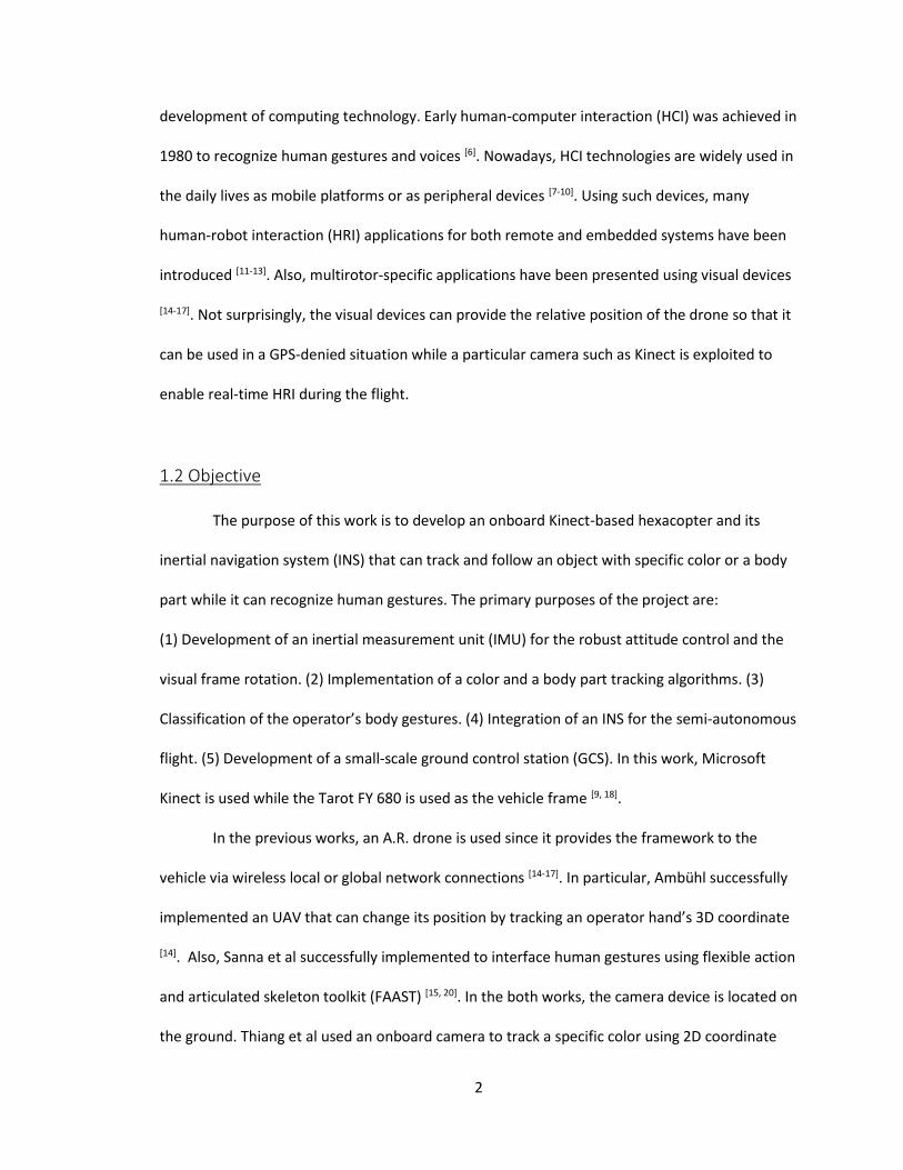
3.3.2 Magnetometer
Three DOF magnetometer measures Earth magnetic fields. Since both gyroscope and
accelerometer are not capable of providing heading estimation, a magnetometer is used to
provide heading information. There is an issue to be addressed for the reliable estimation of
heading. The magnetometer’s raw data is decentered due to a bias as shown in Figure 3.4. The
bias is the result of local magnetic field varying by the given environment for the installation and
operation of the vehicle [38]. Yet, once the sensor is calibrated, the variation during flight is small
[38].

24
(a) Raw magnetometer value Y vs X (b) Raw magnetometer value Z vs Y
(c) Raw magnetometer value X vs Z
Figure 3.4 Raw magnetometer value distribution
To re-centralize, max and min values are selected from each axis, and their mean value is
calculated since the mean value indicates the magnitude of the off-center. For the plots
presented here, the offset is computed as 9, -167, and 23 for x, y, and z axis each as shown in
figure 3.5.

25
(a) Corrected magnetometer value Y vs X (b) Corrected magnetometer value Z vs Y
(c) Corrected magnetometer value X vs Z
Figure 3.5 Corrected magnetometer value distribution
3.4 Complementary Filter
As noted in chapter 3.3, the immediate use of raw values of the sensor does not provide
a robust and consistent estimation of the vehicle state. To achieve robust estimation, a
complementary filter using the rotation matrix is employed in this project [37]. The rotation
matrix provides reliable estimation than equations 3.1 and 3.2 since the estimation is based on
angular velocity while the error can be corrected by using the acceleration and heading.

26
3.4.1 Rotation Matrix Construction
Assuming that the body is resting on the ground at the begging, rotation matrix can be
initialized using equations 3.7 and 3.8 since the three equations output ϕ, θ, 𝑎𝑛𝑑 ψ.
[𝑅]𝑖
= [
cos(𝜃) co s( 𝜓) sin(𝜙) cos(𝜃) − cos(𝜙) si n( 𝜓) cos(𝜙) sin(𝜃) cos(𝜓) + sin(𝜙) si n(𝜓)
cos(𝜃) si n( ψ) si n(𝜙) cos(𝜃) sin(𝜓) + cos(𝜃) co s( 𝜓) cos(𝜙) sin(𝜃) sin(𝜓) − sin(𝜙) co s(𝜓)
−si n( 𝜃) si n( 𝜃)co s( 𝜃) co s(𝜙)co s( 𝜃)]
After establishing initial rotation matrix, next rotation matrix can be constructed by using
angular velocities from the gyroscope.
[𝑅]𝑖+1 = [𝑅]𝑖 ( [𝐼] + [
0 −𝜔𝑧 𝜔𝑦
𝜔𝑧 0 𝜔𝑥
−𝜔𝑦 −𝜔𝑥 0]
𝑖
× ∆𝑡 ) (3.11)
where
[𝐼] is identity matrix.
Since the raw values of angular velocity from the gyroscope do not conserve orthogonality, the
rotation matrix does not conserve orthogonality as well. Therefore, the correction for preserving
orthogonality needs to be addressed. The following equations correct orthogonality since the
rotation matrix is symmetric and orthogonal.
𝐸 = [𝑅1]𝑇[𝑅2] (3.12)
where
𝐸 is orthogonality error,
[𝑅1] is the first column of [𝑅]𝑖, 𝑒𝑎𝑟𝑡ℎ, and
[𝑅2] is the second column of [𝑅]𝑖, 𝑒𝑎𝑟𝑡ℎ
Since the error is calculated by dot product of first two columns, error can be equality divided
and subtracted to each column vectors.
[𝑅1]𝑜𝑟𝑡ℎ = [𝑅1] −𝐸
2[𝑅2] (3.13)

27
[𝑅2]𝑜𝑟𝑡ℎ = [𝑅2] −𝐸
2[𝑅1] (3.14)
where
[𝑅1]𝑜𝑟𝑡ℎ is the orthogonalized vector of the first column of [𝑅]𝑖, 𝑒𝑎𝑟𝑡ℎ, and
[𝑅]𝑜𝑟𝑡ℎ is the orthogonalized vector of the second [𝑅]𝑖, 𝑒𝑎𝑟𝑡ℎ
Since the rotation matrix has to keep orthogonality for all axes, the third column of [𝑅]𝑖, 𝑒𝑎𝑟𝑡ℎ
can be calculated by using cross product of first two orthogonalized column vectors.
[𝑅3]𝑜𝑟𝑡ℎ = [𝑅1]𝑜𝑟𝑡ℎ × [𝑅2]𝑜𝑟𝑡ℎ (3.15)
As a result, [𝑅] can be expressed as below.
[𝑅]𝑜𝑟𝑡ℎ = [ [𝑅1]𝑜𝑟𝑡ℎ [𝑅2]𝑜𝑟𝑡ℎ [𝑅3]𝑜𝑟𝑡ℎ ] (3.16)
Finally, each row of the rotation matrix needs to be scaled to one. Since magnitude of each row
does not significantly vary from one, Taylor expansion can be used to renormalize the rows.
[𝑅1]𝑛𝑜𝑟𝑚 =1
2(3 − [𝑅1]𝑜𝑟𝑡ℎ ∙ [𝑅1]𝑜𝑟𝑡ℎ)[𝑅1]𝑜𝑟𝑡ℎ (3.17)
[𝑅2]𝑛𝑜𝑟𝑚 =1
2(3 − [𝑅2]𝑜𝑟𝑡ℎ ∙ [𝑅2]𝑜𝑟𝑡ℎ)[𝑅2]𝑜𝑟𝑡ℎ (3.18)
[𝑅3]𝑛𝑜𝑟𝑚 =1
2(3 − [𝑅3]𝑜𝑟𝑡ℎ ∙ [𝑅3]𝑜𝑟𝑡ℎ)[𝑅3]𝑜𝑟𝑡ℎ (3.19)
3.4.2 Error Correction
As indicated earlier, the orthogonalization and the renormalization do not guarantee
robust estimation of the rotation since the source values; the angular velocities of three axes
have noise. Even though the noise at a point is insignificant, as the integration processes iterate,
the error will accumulate, and this can lead to significant amount of drift of the rotation matrix.
To be able to estimate vehicle attitude, the drift needs to be corrected. The accelerometer and
the magnetometer are used as reference sources for the correction.

28
Since rotation matrix conserves rotation through the rotation axes, when body frame
accelerometer is given, earth frame acceleration should indicate the gravitational acceleration
vector, i.e. [0 0 −9.81] 𝑚/𝑠2, assuming that the rotation matrix has no error due to the
sensor noise. However, often time, the rotated body frame to earth frame acceleration vector is
not exactly equal to the gravity vector. By contradiction to the assumption that the rotation
matrix is correct, the rotation matrix has error whenever the ground frame acceleration vector
is not equal to the gravitational acceleration vector. Using cross product, the magnitude of the
error in x and y axes rotation angles between the gravity vector and the ground frame
acceleration vector with the drift can be computed.
[Exy] = [ACCearth] × [𝐺] (3.20)
where
[Exy] is the error vector in the ground frame due to the drift and the z component is 0,
[ACCearth] is ground frame acceleration, and
[G] is gravity vector, [0 0 g], where g = -9.81 m
s2
To calculate z component of rotation error regarding ground frame, magnetometer data can
be incorporated in a similar manner. Since default heading is set to the North, i.e.[1 0 0],
ground frame magnetometer should indicate the North. Otherwise, it reveals the error due to
the drift of z axis gyroscope value.
[Ez] = [𝑀𝐴𝐺𝑒𝑎𝑟𝑡ℎ] × [𝑁𝑜𝑟𝑡ℎ] (3.21)
where
[Ez] is z components of error in the ground frame due to drift,
[MAGearth] is ground frame heading, and
[North] is heading vector for the North, [1 0 0].

29
By adding the two error vectors in ground frame, the total error vector in ground frame
perspective can be constructed and rotated back to the body frame for the correction.
[E]earth = [𝐸𝑥𝑦] + [𝐸𝑧]
[E]body = [𝑅′]𝑛𝑜𝑟𝑚 [𝐸]𝑏𝑜𝑑𝑦 (3.22)
Eventually, the error information is fed for proportional integral (PI) compensator by
constructing a new rotation matrix based on the error.
[R]cor = [𝑅′]𝑛𝑜𝑟𝑚 ([𝐼] + [
0 𝐸𝑧 −𝐸𝑦
−𝐸𝑧 0 𝐸𝑥
𝐸𝑦 −𝐸𝑥 0] × 𝐾𝑝) (3.23)
where
[R]cor is corrected rotation matrix,
Ex is x element of the body frame error vector,
Ey is y element of the body frame error vector,
Ez is z element of the body frame vector, and
Kp is the proportional gain of PI compensator.
Also, to prevent further error due to gyroscope bias, error integration can be considered by
accumulating the error and subtracting it for the next iteration.
[E]acc = [𝐸]𝑎𝑐𝑐 + 𝐾𝑖 [𝐸]𝑏𝑜𝑑𝑦 (3.24)
[
𝜔𝑥
𝜔𝑦
𝜔𝑧
] = [
𝜔𝑥, 𝑟𝑎𝑤
𝜔𝑦, 𝑟𝑎𝑤
𝜔𝑧, 𝑟𝑎𝑤
] − [𝐸]𝑎𝑐𝑐 (3.25)
where
[E]acc is accumulated error in the body frame, and
Ki is integral gain of the PI compensator.

30
3.5 Results
3.5.1 Simulation Result
Figures 3.6-3.8 show the Matlab-based CF algorithm results.
Figure 3.6 CF estimation of pitch, simulation output
Figure 3.7 CF estimation of roll, simulation output

31
Figure 3.8 CF estimation of yaw, simulation output
3.5.2 Implementation
In this section, how the above algorithm has been implemented on the IMU is discussed.
Since the sampling rates of the sensors are different, four cogs of the MCU have been exploited
to process the CF routines while preserving the original sampling rates of the sensors. Also, to
share the memory space with other MCUs, three cogs are used as shown in figure 3.9.
Figure 3.9 IMU Structure

32
To read each sensor, I2C protocol is used. Although I2C protocol allows the line to read several
sensors, the sampling rate decreases since several sensors are using the communication lines.
By using different cogs, the sampling rates for the CF algorithm are 175 Hz for the gyroscope,
130 Hz for the accelerometer, and 10 Hz for the magnetometer.
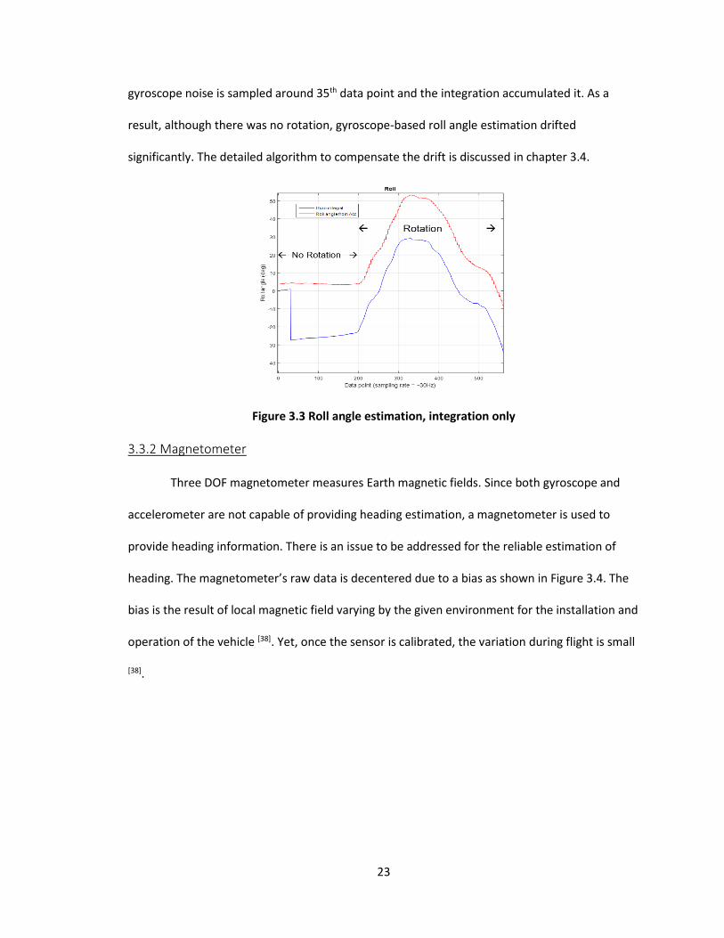
Preprocessing is required since the raw magnetometer values contain noise, which can
result in uncertainties in estimation as shown in figure 3.10 [38]. Similarly, the accelerometer
values go through an average filter, which outputs the average value of the data at 13Hz as
shown in figure 3.11.
(a) Raw magnetometer signals (b) Low pass filtered magnetometer signals
Figure 3.10 Magnetometer signals
33
Figure 3.11 Average filtered accelerometer signals
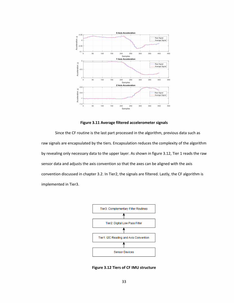
Since the CF routine is the last part processed in the algorithm, previous data such as
raw signals are encapsulated by the tiers. Encapsulation reduces the complexity of the algorithm
by revealing only necessary data to the upper layer. As shown in figure 3.12, Tier 1 reads the raw
sensor data and adjusts the axis convention so that the axes can be aligned with the axis
convention discussed in chapter 3.2. In Tier2, the signals are filtered. Lastly, the CF algorithm is
implemented in Tier3.
Figure 3.12 Tiers of CF IMU structure

34
3.5.3 Experimental Result
In this section, the IMU data output is presented. The same CF algorithm is used as
chapter 3.5.1. The only difference is that Parallax Propeller MCU does not support primitive
floating point types. To conserve the computing speed, 32 bit signed long type variables are
exclusively used. Figures 3.13 – 3.15 show the results from MCU implementation. The output of
the CF (green line) at each axis shows that Euler angle estimation has less noise and drift with
negligible phase shift.
Figure 3.13 CF estimation of pitch, IMU output

35
Figure 3.14 CF estimation of roll, IMU output
Figure 3.15 CF estimation of yaw, IMU output

36
Chapter 4. Vision Sensor and Flight Management Computer
4.1 Color Tracking
In this chapter, object and body tracking methods are discussed. Microsoft Kinect is a
camera mounted onboard. The camera provides 30 fps RGB, infrared, depth, and skeletal
frames. Tracking a target or estimating relative coordinates of the target is an important process
for the drone to navigate in the GPS-denied situation. For this system, a set of computer vision
algorithms is exclusively applied as a surrogate position estimator. To aid taking off, landing, or
navigation, a color detection algorithm is implemented using Microsoft Kinect SDK 1.7 (MSKSDK)
and EmguCV [39]. The color detection algorithm uses RGB and depth frames to estimate the 3D
coordinate of a red object. Figure 4.1 shows the flow of the color detection routines. The
routines in green are presented in the following sections and INS part is discussed in Chapter 5.
Figure 4.1 Color detection routines

37
4.1.1 Color Space Conversion
The MSKSDK can output an RGB frame in bitmap format using a byte array. OpenCV
then creates an RGB image matrix. However, RGB frame can be misleading because RGB color
space is nonlinear [40]. Especially, brightness change in the RGB space results in having different
hues. The light intensity varies by the angle and the position of the camera. During the drone
operation, the onboard camera is exposed to the structural vibration, attitude noise, and
continuously changing position. Therefore, for the robustness of the color detection algorithm,
RGB color space needs to be converted to hue-saturation-value (HSV) color space. With HSV
frame, thresholding can be operated regardless of change of light intensity. In HSV frame, hue is
the type of color, saturation is the chroma, and value represents the brightness as shown in
Figure 4.3. Therefore, HSV frame provides abundant information regarding the pixels in the
frame.
Figure 4.2 RGB Color Space

38
Figure 4.3 HSV Color Space
In EmguCV, CvInvoke.cvtColor(InputArray src, OutputArray dst, int code) function is
used to convert the color space. The first argument is the RBG image array and the second one
is the empty array that will contain the converted HSV image. The last argument of the function,
“code”, is ColorConversion enumerator. In this case, ColorConversion.Rgb2Hsv is passed. Figure
4.4 illustrate the color space conversion. In figure 4.4 (a), 10% of the noise is artificially added to
emualte noisy flight environment.
(a) Noisy Image in RGB color space (b) Converted image in HSV color space
Figure 4.4 RGB (a) and HSV (b) images

39
4.1.2 Thresholding
The “red” pixels in RGB frame are converted to the certain ranges of literals in the HSV
frame. The red hue value is around 160 – 179 [39]. The saturation and the brightness are adjusted
experimentally since they differ by the environments. To detect the pixels of the object of
interest, in this case, red, thresholding routines are processed. The thresholding is process on
the each axis of the HSV frame. For the hue axis, the values between 110 and 160 are passed at
the specific lab environment for the red pixels. The passed pixels are represented by 1 or 0
otherwise as shown in figure 4.5. Similarly, the saturation and value frames are thresholded as
figures 4.6 - 4.7 show.
(a) Hue frame (b) Thresholded hue frame
Figure 4.5 Hue frame filter
(a) Saturation frame (b) Thresholded saturation frame
Figure 4.6 Saturation frame filter

40
(a) Value frame (b) Thresholded value frame
Figure 4.7 Value frame filter
Eventually, the filtered frames are overlapped and their binary pixels are merged by bit-wise
AND-gates. Figure 4.5 shows the resultant frame.
Figure 4.5 AND gated filtered image
4.1.3 Morphological Operation
Since the noise in the resultant frame is significant, the small white dots can be
eliminated by morphological opening. Unless the noise are not reduced, the contour algorithm
needs lots of computations since the algorithm has to iterate every white pixels in the frame.

41
Such excessive iterations can end up with the delaying the process. The opening process is
morphological erosion followed by dilation. By eroding the pixels, minimal kernels are left [42].
Dilation is the reverse process of erosion. Using EmguCV, CvInvoke.Erode() and CvInvoke.Dilate()
are operated. The result frame that morphological opening is process is presented in figure 4.6
(a). Also, to fill the small black holes in the white blob, morphological closing is operated based
on the figure 4.6 (a). It is shown in figure 4.6 (b).
(a) Morphologically opened frame (b) Morphologically closed frame
Figure 4.6 Morphological operations of the frame
4.1.4 Contour and Relative Coordinate Estimation
To locate the largest white blob in figure 4.6, CvInvoke.findContours() is used [34, 35, 43].
The function returns the array of contour information of all white blobs in figure 4.6. The
information includes 2D vector position of the contour, width, height, and area. Since the
significant white blob’s area is usually larger than 500, other small white blobs can be
suppressed as shown in figure 4.7.

42
Figure 4.7 The contour of the largest white blob
Using the information provided by CvInvoke.FindContours(), the red object in the input frame
can be located as figure 4.8.
Figure 4.8 Red object detection, marked by a blue rectangle
Based on the 2D coordinate from the RGB frame, the depth, or the X axis coordinate of
the object can be calculated using the depth frame from the Kinect. The depth frame has one
channel whose values span from 0 to 255. The higher value means the further pixels (see figure

43
4.9). Although the size of the depth frame is slightly smaller than the RGB frame, the error is
negligible when the 2D coordinate of the red object from the RGB frame is overlaid to calculate
the depth of the object.
Figure 4.9 Depth frame
The depth is calculated by averaging the pixels in the contour area. Yet, the depth
information is not the x coordinate of the object because the depth frame only offers the
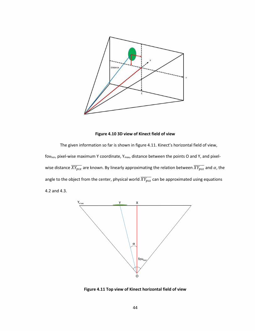
distance (See figure 4.10) [46]. The calculation of the X coordinate can be simply done by
Equation 4.1. However, the y and z coordinate value is in pixel-wise unit while the depth frame
can be directly converted to physical unit such as meter. Therefore, the conversion from pixel to
real-world unit needs to be processed before the x coordinate calculation.
x coordinate = √Distance2 − 𝑦2 − 𝑧2 (4.1)
44
Figure 4.10 3D view of Kinect field of view
The given information so far is shown in figure 4.11. Kinect’s horizontal field of view,
fovhor, pixel-wise maximum Y coordinate, Ymax, distance between the points O and Y, and pixel-
wise distance 𝑋𝑌𝑝𝑖𝑥 are known. By linearly approximating the relation between 𝑋𝑌𝑝𝑖𝑥
and 𝛼, the
angle to the object from the center, physical world 𝑋𝑌𝑝𝑖𝑥 can be approximated using equations
4.2 and 4.3.
Figure 4.11 Top view of Kinect horizontal field of view

45
𝛼 ≈ 𝑋𝑌𝑝𝑖𝑥
𝑋𝑌𝑚𝑎𝑥,𝑝𝑖𝑥 ×
𝑓𝑜𝑣ℎ𝑜𝑟
2 (4.2)
𝑋𝑌𝑝ℎ𝑦 = sin(𝛼) × 𝑂𝑌𝑝ℎ𝑦
(4.3)
where
fovhor is 62 degree [44] and
the frame size in pixel is 640 by 480 (width by height).
Since the maximum depth that Kinect can sense is 3 meters, the maximum possible error of the
X coordinate due to linear approximation using equations 4.1 - 4.3 is approximately 5 cm. Z
coordinate conversion can be done in the same manner. 49 degree is used for the vertical field
of view [44].
4.2 Body Part Detection
MSKSDK offers body parts’ 3D coordinates. Figure 4.12 shows types of the body parts
available in MSKSDK. Since the coordinate system is different from the definition in chapter 3,
the axes need to be changed correspondingly. In this project, left and right hand and spine
coordinates are used for the simplicity.

46
Figure 4.12 Kinect skeletal body part [9]
4.3 Human Robot Interaction
For the drone operation, the MS Kinect can receive the input as a form of gestures.
Based on the body parts’ coordinates retrieved in the previous section, skeletal and motion
recognition algorithm is implemented using a kernel method and an artificial neural network
(ANN). The rule-based algorithms such as nested if statements and for loops are not resilient
enough to recognize a certain pattern, which differs every time. Due to the changing pattern,
the rule-based algorithm does not output the robust results. When the output is not the desired
result, the vehicle and the operator can be exposed to the serious damage.
Unlike the rule-based algorithm, ANN can process the pattern fast and classify the
pattern with great resilient and thus the output has the high accuracy. Yet, the misclassification

47
as an output can result in the damage as well. To wrap the input gesture, a finite state machine
is used. The overall algorithm is presented in figure 4.13.
Figure 4.13 Kinect-based body gesture input algorithm
4.3.1 Human-Noise Skeletal Classification
The Kinect’s original body part recognition algorithm is internally implemented in
MSKSDK. Therefore, the MSKSDK merely outputs the skeletons recognized by the depth frame
[47]. Since for the most of the time, Kinect is installed on a fixed object such as TV stand or a
monitor, the probability of recognition of non-human object as a human is infrequent. However,
Kinect is mounted on a drone in this project, and the flight causes vibrations, drifting, and
rotation of the camera frame. Due to this reason, it is more likely for the internal depth frame-
based body part recognition algorithm to output a set of body parts although it is not actually
from a human in front of the camera. Without the human-noise classifier, the mere output of
the skeletal frame can be misleading. Figure 4.14 shows a few sets of the skeletal frames before
the classification. If the skeletal points due to the noise get into the gesture classifier, the
untoward input from the noise skeleton can execute a command for the drone regardless of the
operator’s intention.

48
(a) Skeletal points on human body
(b) Skeletal points due to noise
Figure 4.14 Unfiltered skeletal frames
For the data input for the classifier, left, center, and right shoulder and hip, head, and
spine 3D coordinates are used. Since the raw relative coordinate of the 3D coordinates can vary
as the position of the operator, all body part coordinates are convered to relative-to-center-
shoulder. For instance, the center shoulder 3D coordinate changes as the operator’s relative
position to the camera changes while the other parts such as left hand 3D coordinate is always
relative to the operator’s centor shoulder location. Next, the collected body parts’ 3D

49
coordiantes are put into a linear array. Since 7 body parts are used, the array size is 21. At the
last column, or at 22nd column, the index of the corresponding class is attached. In this project, 1
is used for the coordinates from the actual human body parts while -1 is used for the
coordinates due to the noise.
The human-noise classification algorithm employes kernel method to differentiate
acutal human skeleton coordinates from those of noise [48,49]. In this project, Gaussian kernel is
used.
K(xi, xj) = 𝑒−
||𝑥𝑖−𝑥𝑗||2
2𝜎2 (4.4)
where xi and xj are the ith and jth data of the training set and 𝜎 is standard diviation of the
Gaussian kernel. Then the optimization objective can be set as below representer theorem.
f ∗ = 𝑎𝑟𝑔min𝑓 ∈𝐻
1
𝑛∑ 𝑉(𝑓(𝑥𝑖), 𝑦𝑖) + 𝜆‖𝑓‖𝑛
𝑖=1 (4.5)
where
𝑓∗is the optimal linear combination of the Gaussian kernel function that predicts the
label,
𝑓(𝑥𝑖) = 𝛼𝐾(𝑥, 𝑥𝑖) where α is n − dimensional vector
yi is the actual label,
V is the loss function, 𝑉 =1
2(𝑓(𝑥𝑖) − 𝑦𝑖)
2,
n is for the number of data points in the training set,
𝜆 is a constant for regularization, and
||𝑓|| is a magnitude of the function values, it is used for the regularization.
The function f(x) will be used to predict the label of the skeletal coordinates of the body parts
during the operation. The regularization term is added to penalize the functions that would
over-fit the train data set. The equation 4.5 can be solved as shown in steps a) and b).

50
Step a) Solving the loss function
1
𝑛∑ 𝑉(𝑓(𝑥𝑖), 𝑦𝑖)
𝑛𝑖=1 =
1
n𝛼𝑇𝐾2𝛼 −
2
𝑛 𝛼𝑇𝐾𝑦 +
𝑦𝑇𝑦
𝑛 (4.6)
Step b) Solving for the regularization term
‖𝑓‖ = ‖∑𝛼𝑖𝐾(𝑥𝑖 , 𝑥𝑖𝑛𝑝𝑢𝑡 )‖2
= αT𝐾 𝛼 (4.7)
Therefore, equation 4.5 can be reduced to
f ∗ = 𝑎𝑟𝑔min𝛼
1
n𝛼𝑇𝐾2𝛼 −
2
𝑛 𝛼𝑇𝐾𝑦 +
𝑦𝑇𝑦
𝑛 + 𝜆 𝛼𝑇𝐾𝛼 (4.8)
To find the argument, α, that minimizes the function, the derivative is taken with respect to α.
2
n𝐾2𝛼 −
2
𝑛𝐾𝑦 + 2𝜆𝐾𝛼 = 0 (4.9)
Finally, α can be found.
α = (K + λnI)−1𝑦 (4.10)
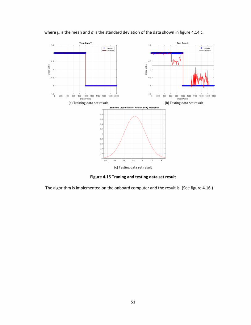
To adjust λ and 𝜎, cross validation is used [45, 48]. Figure 4.15 shows the results of the training and
testing. The predicted values euqal to and larger than zero can be regarded as actual human
skeletal coordinates while the values less than zero can be regarded as the skeletal coordinates
from the noise.
The skeletal data due to noise can vary significantly as shown in figure 4.15b. That taking
the boundary simple as 0 may not produce good prediction accuracy. Therefore, another
constraint needs to be set to determine which can be regarded as the class with the index 1.
From the figure 4.15 b, the labeled data’s prediction result’s distribution is shown in figure 4.15
c. For the specific data set shown here has the mean as 0.8313 with standard deviation of
0.2319. With confidence interval with 99%, the range can be deteremined as 0.9863 and 1.008
using equation 4.11 [50].
(μ − 2.575 × σ, μ + 2.575 × σ ) (4.11)
51
where μ is the mean and σ is the standard deviation of the data shown in figure 4.14 c.
(a) Training data set result (b) Testing data set result
(c) Testing data set result
Figure 4.15 Traning and testing data set result
The algorithm is implemented on the onboard computer and the result is. (See figure 4.16.)

52
(a) Skeletal points of the human (b) Skeletal points due to noise
(c) Classification result based on human body parts (d) Classification result based on the noise
Figure 4.16 Human-noise classification result
4.3.2 Gesture Recognition
A single hidden layered ANN algorithm is implemented for the gesture classification
algorithm. As an input data, an operator’s body parts coordinates are collected and labeled. The
labels indicate the class type. In this project, take off, proceed, retreat, and landing gesture
inputs are used.
4.3.2.1 Neural Network Design
The neural network implemented in this project has single hidden layer and one output
layer as shown in figure 4.17. All neurons have bias connection. Hidden neurons use tangent

53
sigmoid function (equation 4.12) and output neurons have softmax function (equation 4.13) for
their activation functions.
tansig =2
1+𝑒−2𝑣 − 1 (4.12)
softmax =ev
∑𝑒𝑣 (4.13)
where v is the dot product of input and weight vectors.
Figure 4.17 Artificial neural network, bias not shown
The forward propagation of ANN is expressed in equations 4.14 and 4.15.
𝑡ℎ𝑒 𝑖𝑡ℎ𝑛𝑒𝑢𝑟𝑜𝑛 𝑜𝑢𝑡𝑝𝑢𝑡 𝑖𝑛 𝑡ℎ𝑒 ℎ𝑖𝑑𝑑𝑒𝑛 𝑙𝑦𝑎𝑒𝑟 = tansig(x ∙ w h,i) (4.14)
𝑡ℎ𝑒 𝑗𝑡ℎ 𝑛𝑒𝑢𝑟𝑜𝑛 𝑜𝑢𝑡𝑝𝑢𝑡 𝑖𝑛 𝑡ℎ𝑒 𝑜𝑢𝑡𝑝𝑢𝑡 𝑙𝑎𝑦𝑒𝑟 = 𝑠𝑜𝑓𝑡𝑚𝑎𝑥(ℎ ∙ �� 𝑗) (4.15)

54
where x is input vector in R180 and wh,i is the weight vector of ith neuron in the hidden layer
and ℎ is the output vector of the hidden layer. In this project, bias is incorporated at every 0th
element of the input vectors for each layer.
4.3.2.2 Data Preprocessing
The input data is composed of two 3D vectors, left and right hand coordinates. During
the flight, it can be confusing for the computer when the movement of the vehicle causes the
relative movement of the body parts. To avoid this, the body part coordinate is subtracted by
the mid-spine coordinate so that the other body parts coordinates are fixed relative to the mid-
spine coordinate. Then these 3D vectors are collected for 1 second. Since the Kinect can offer
the data at 30 Hz, total 30 data points are collected. Then the data set is linearly attached as an
array with dimension of 180. Also, this array needs to be scaled from -1 to 1 to normalize the
value. For the normalization mapminmax() function is used in Matlab and implemented in C# for
the real-time computation. The function definition is shown in equation 4.16.
𝑚𝑎𝑝𝑚𝑖𝑛𝑚𝑎𝑥(𝑖𝑛𝑝𝑢𝑡 ) =(1−(−1))×(𝑖𝑛𝑝𝑢𝑡 −min(𝑖𝑛𝑝𝑢𝑡 ))
max(𝑖𝑛𝑝𝑢𝑡 )−min (𝑖𝑛𝑝𝑢𝑡 )+ (−1) (4.16)
where
𝑖𝑛𝑝𝑢𝑡 is the 180-dimensional array.
In equation 4.16, 1 and -1 is used for the maximum and minimum values of the normalized
array.
4.3.2.3 Training
The training process of the ANN is locating the minimum of the cost function. Although
the algorithm can be stuck in a local minimum, in practice, resulting in global minimum is

55
frequent by randomizing the order of data [8]. The error and the error energy function at nth
epoch is defined as equation 4.17 and 4.18 [41].
ek(𝑛) = 𝑑𝑘(𝑛) − 𝑦𝑘(𝑛) (4.17)
Ek(𝑛) =1
2𝑒𝑘
2(𝑛) (4.18)
where
dk is the label or desired output of the kth input vector, and
yk is the output of the forward propagation of the kth input vector.
By summing the error energy functions by all data point, the total cost function is defined and
gradient descent rule is applied [45].
𝐸(𝑛) =1
2∑ [𝑑𝑘(𝑛) − 𝑦𝑘(𝑛)]2𝑘 =
1
2∑ [𝑑𝑘(𝑛) − 𝜓(∑ 𝑤𝑘𝑗𝑦𝑗𝑗 )]
2𝑘 (4.19)
where
𝜓 is the activation function of a neuron, and
j is jth neuron from the previous layer.
To find the minimum error energy function, the partial derivative can be taken with respect to
weight.
∂E
∂wkj= −ek𝜓
′(𝑣𝑘)𝑦𝑗 (4.20)
Therefore, the weight vectors of output layer at (n+1)th iteration is
𝑤𝑘𝑗(𝑛 + 1) = 𝑤𝑘𝑗(𝑛) + 𝜂𝑒𝑘(𝑛)𝜓′(𝑣𝑘)𝑦𝑗(𝑛) (4.21)
Similarly, weight update for the hidden layer can be calculated.
𝑤𝑗𝑖(𝑛 + 1) = 𝑤𝑗𝑖(𝑛) + 𝜂𝜓′ (𝑣𝑗(𝑛)) [∑ 𝑤𝑘𝑗(𝑛)𝑘 𝑒𝑘(𝑛)𝜓′(𝑣𝑘)]𝑥𝑖(𝑛) (4.22)
where
i indicates ith input.

56
In Matlab, Pattern Net in the Neural Network toolbox is used to expedite the back
propagation process. Then, the weight vectors of the Matlab is imported to the Kinect software
in C# so that the real-time body coordinates can be fed into the forward propagation algorithm
shown the previous chapter. For the training, 2000 data points are collected for each class.
Therefore, 8000 data points are collected in total for the four different classes of the body
gesture: take-off, landing, proceed, and retreat with the corresponding labels of 1, 2, 3, and 4
respectively. Figure 4.18 shows the gesture labels.
(a) Class1: idle gesture (b) Class2: take off / landing gesture
(c) Class3: proceed gesture (d) Class4: retreat gesture
Figure 4.18 Gestures of four classes
The Matlab’s toolbox shows the training process in Cross-Entropy, figure 4.19.

57
Figure 4.19 Training performance
Since the body gestures used in the project is only 4 types with distinctive space and with a
steady camera, the accuracy can be 100 percent. Figure 4.20 shows the classification result.
Figure 4.20 Classification result of the training (left) and testing (right) sets
4.3.3 Finite State Machine
A finite state machine (FSM) is used to suppress misclassification result during the
operation. The misclassification is primarily due to the noise generated by the moving frame.

58
Also, when a body part is not detected or outside of the frame, Kinect’s built-in body part
recognition algorithm’s estimation accuracy can drastically deteriorate, which results in
outputting the 3D coordinates with low accuracy.
The FSM has three states in this project: ground, preflight, and tracking as shown in
figure 4.21. FSM can receive any input. Yet, it reacts to specific sets of input. Table 4.1 lists the
states, inputs, and outputs of the FSM. Since FSM only reacts to a certain input types, it is safe
to interface the INS because wrong input (ANN misclassification) can be directly sent to the INS,
which does not have the algorithm for context-depending decision rules, and the wrong input
can cause malfunctioning during the operation. Such unexpected operation can result in
structural damage.
Figure 4.21 Finite state machine for 4 different flight modes

59
Table 4.1 State Transition Table
Current State Possible Input Output Next State
Ground
none none Ground
take off turn on attitude PID Controller Preflight
landing none Ground
proceed none Ground
retreat none Ground
time elapse none Ground
Preflight
none increase throttle Preflight
take off none Preflight
landing none Preflight
proceed none Preflight
retreat none Preflight
time elapse turn on position PID controller Tracking
Tracking
none none Tracking
take off none Tracking
landing lower height setpoint Tracking
proceed decrease distance setpoint Tracking
retreat increase distance setpoint Tracking
time elapse none Tracking
Landing
Distance <= 30 ? turn off PID controllers Ground
distance > 30 ? decrease throttle Landing
take off none Landing
landing none Landing
proceed none Landing
retreat none Landing
time elapse none Landing
In figure 4.21, the human input is the output of the ANN classification result. ANN can output
FSM input such as “take off”, “proceed”, “retreat”, and “land”. The automatic input is generated
by the specific state that is not accessible by an operator during the mission. During the
inaccessible states such as “Preflight” and “Landing”, the FMC iterates an open and closed loops
respectively. During the state of “Preflight”, FMC sends messages to INS to gradually increase
the throttle to a pre-determined pulse width modulation (PWM) so that the lift generated by
the propellers is slightly lower than the weight. Similarly, during the state of “Landing”, FMC

60
sends messages to gradually decrease the throttle based on the ultrasonic distance sensor
reading. When the distance sensor reading is less than 30cm, the state of “Landing” switches to
the state of “Ground”.

61
Chapter 5. Inertial Navigation System
5.1 Introduction
This chapter discusses how the IMU is integrated with other MCUs (See figure 5.1). Since single
Parallax Propeller module has 8 cogs, to parallel-process several routines during the mission,
inertial navigation system (INS) in this project needs four MCU boards. The first module is used
for IMU, discussed in chapter 3. Other important aspects of the navigation system are controller
and data sharing with each other. In chapter 5.2 and 5.3, the controller and the data sharing
algorithm is presented. Communications with the ground control station and flight management
computer is discussed in chapter 6.

62
Figure 5.1 Parallax Propeller microcontroller-based inertial navigation system

63
5.2 PID Controller / ESC Driver Implementation
5.2.1 ESC Driver
Pulse width modulation (PWM) is a digital signal that contains the information regarding
duty cycle. For a motor control, duty cycle can be viewed as a variable controlling the RPM of
the motor. As shown in figure 5.2, 10 or 50 percent of duty cycle outputs the corresponding
percentage of the maximum RPM of the motor.
Table 5.1 Pulse width modulation generation for a motor
1 initialize pin // a pin to output the signal 2 initialize highTime // time for the high signal. ex) 0.5 for figure 5.2 (b) 3 repeat 4 set high signal for a pin 5 maintain the high signal for highTime 6 set low signal for a pin 7 wait for ( period - highTime ) // keeping the exact period
(a) 10 percent duty cycle (b) 50 percent duty cycle
Figure 5.2 Pulse width modulation, period = 1 second
As presented in chapter2, the electric speed controller (ESC) used in this project can
receive the signal with frequency between 30 to 450 Hz, or with the periods of 0.0022 to 0.0333
seconds. For the best efficiency of the INS, the input frequency is set as 150Hz because the
maximum update rate of the IMU is 150Hz. Also, for the single motor, the maximum time for the
high signal is approximately 0.002 second, which is slightly shorter than the minimum period. To

64
operate the 6 ESCs at 0 to 100 percentage of the capacity, using one cog of the MCU cannot be
sufficient. As shown in Table5.2 line 9, the possible total time elapse can be 0.002 × 6 = 0.012
second, which is longer than 0.006 second, the period for 150 Hz. To maintain 150Hz input, two
cogs of the MCU have to be exploited. Each cog operates 3 ESCs. Therefore, the array size in
Table 5.2 line 1 and 2 is 3 rather than 6 while the same code is used for another cog that
controls the rest of the three motors.
Table 5.2 Pulse width modulation generation
1 initialize pin[6] // initialization of microcontroller’s pins, 6 pins for a hexacopter 2 initialize highTime[6] // initialization of the time elapse of the high signal for 6 ESCs 3 repeat 3 initialize totalElapse = 0 // initialization of the variable to store the total highTime 4 for each i 5 set high signal for pin[i] 6 maintain the high signal for highTime[i] 7 set low signal for pin[i] 8 totalElapse += highTime[i] 9 wait for ( period - totalElapse ) // keeping the exact period
To update the RPM, the variable “highTime[i]” needs to be updated. The amount of the change
is calculated by an attitude controller.
5.2.2 Attitude PID Controller
For the stability of the attitude and position of the vehicle, proportional integral
derivative (PID) controllers are implemented [52, 54].
u(t) = Kpe(t) + Ki ∫ e(t)dt + Kdde(t)
dt (5.1)
where, Kp is proportional gain, Ki is integral gain, Kd is derivative gain, e(t) is error signal, u(t) is
the output of the controller, and the function argument t is time. The block diagram of PID
controller and a reduced block is shown in figure 5.3. PID controller receives error signal. The
error is the difference between the reference and sensor signals.

65
Figure 5.3 PID Blocks (left) and reduced block (right)
The proportional block outputs a signal to compensate the error. The magnitude of the
proportional signal is determined by the proportional gain, Kp. To reduce the amount of
overshoot, the derivative block outputs a signal based on the derivative of the error signal with
respect to time. Similarly, the amount of the derivative signal is determined by the derivative
gain, Kd. Lastly, to compensate the steady state error, the integral block outputs the integration
of the error signal. The amount is determined by the integral gain, Ki. Lastly, the total output is
the summation of the outputs from the three blocks.
For the attitude controller, a digital PID controller is implemented. The sensor reading is
based on the IMU. The digital PID controller algorithm is shown in Table 5.3.
Table 5.3 PID controller algorithm
1 repeat 2 for each Euler angle 3 error = reference – current angle 4 proportional = Kp × error
5 derivative = Kd × (error – prev_error) / ∆t 6 integral += Ki × error 7 output = proportional – derivative + integral 8 previous error = error
The attitude PID controller needs the inputs as three Euler angles at each iteration. For
pitch control, motor number 1, 2, 4, and 5 are updated. For Roll control, motor number 1, 2, 3,
4, 5, and 6 are updated. For yaw control, motor number 1, 2, 3, and 5 are updated (See figure
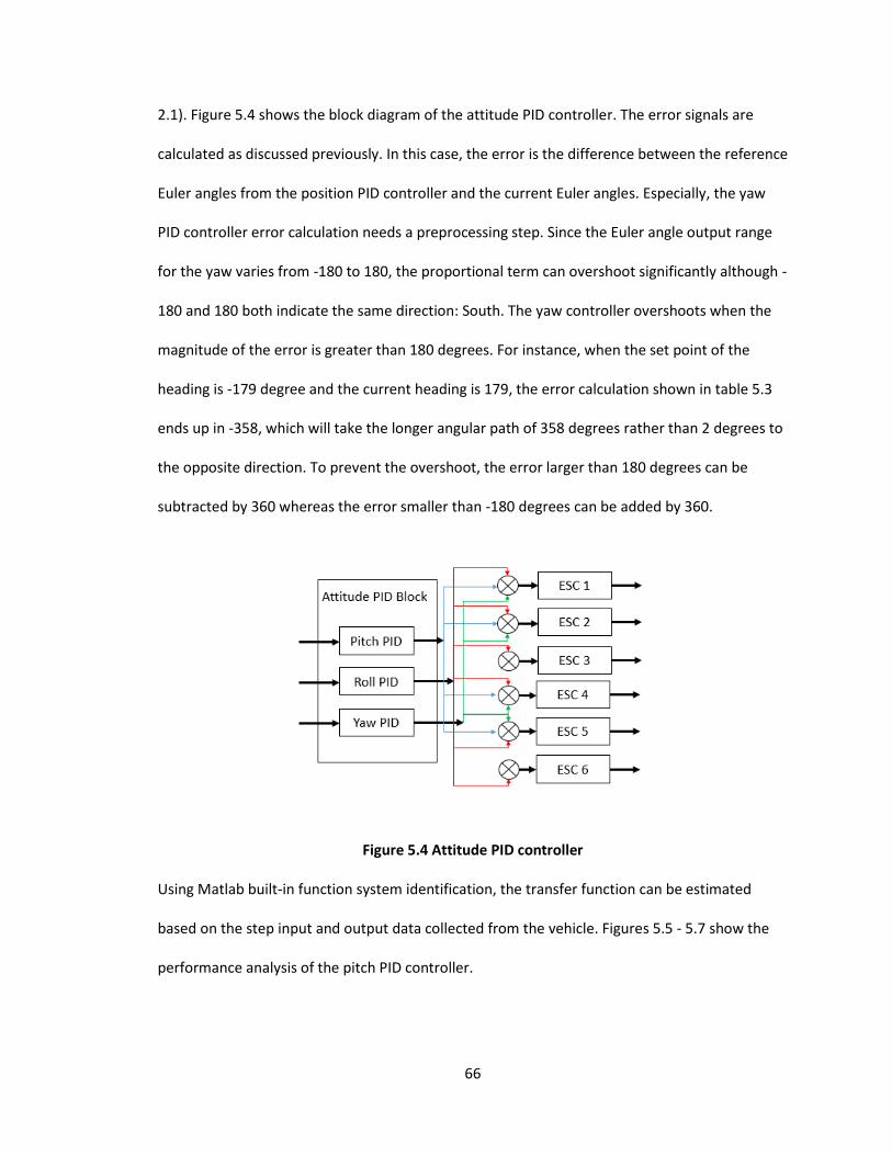
66
2.1). Figure 5.4 shows the block diagram of the attitude PID controller. The error signals are
calculated as discussed previously. In this case, the error is the difference between the reference
Euler angles from the position PID controller and the current Euler angles. Especially, the yaw
PID controller error calculation needs a preprocessing step. Since the Euler angle output range
for the yaw varies from -180 to 180, the proportional term can overshoot significantly although -
180 and 180 both indicate the same direction: South. The yaw controller overshoots when the
magnitude of the error is greater than 180 degrees. For instance, when the set point of the
heading is -179 degree and the current heading is 179, the error calculation shown in table 5.3
ends up in -358, which will take the longer angular path of 358 degrees rather than 2 degrees to
the opposite direction. To prevent the overshoot, the error larger than 180 degrees can be
subtracted by 360 whereas the error smaller than -180 degrees can be added by 360.
Figure 5.4 Attitude PID controller
Using Matlab built-in function system identification, the transfer function can be estimated
based on the step input and output data collected from the vehicle. Figures 5.5 - 5.7 show the
performance analysis of the pitch PID controller.

67
Figure 5.5 Pitch PID controller simulation and experiment output
Figure 5.6 Root locus for the pitch PID controller and plant

68
Figure 5.7 Bode plot for the pitch PID controller and plant
The pitch controller is assumed to be a second order system. The estimated transfer function is
pitch(s) =101
𝑠2+6.848𝑠+95.52 (5.2)
As shown in figures 5.6 and 5.7, the system meets stability criterion [52, 54]. Also, the performance
analysis is listed as below.
Table 5.4 Pitch PID controller performance
Rise Time 0.166 (s)
Settling Time 3.1918 (s)
Overshoot 34.7563 (%)
Peak 1.4389
Peak Time 0.3501 (s)
Gain Margin ∞ (dB)
Phase Margin 56.51 (deg)
Similarly, the roll PID controller is analyzed. Figures 5.8 - 5.10 show the performance analysis of
the roll PID controller.

69
Figure 5.8 Roll PID controller simulation and experiment output
The roll controller is assumed to be second order system. The estimated transfer function is
Figure 5.9 Root locus for the roll PID controller and plant

70
Figure 5.10 Bode plot for the roll PID controller and plant
The performance of the roll PID controller is listed as the table below.
roll(s) =76.26
𝑠2+13.36𝑠+81.8 (5.3)
Table 5.5 Roll PID controller performance
Rise Time 0.3017 (s)
Settling Time 0.6444 (s)
Overshoot 3.1944 (%)
Peak 0.9621
Peak Time 0.5169 (s)
Gain Margin ∞ (dB)
Phase Margin ∞ (deg)
Finally, the yaw PID controller is shown in figures 5.11 - 5.13.

71
Figure 5.11 Yaw PID controller simulation and experiment output
Figure 5.12 Bode plot for the yaw PID controller and plant

72
Figure 5.13 Bode plot for the yaw PID controller and plant
yaw(s) =363.4
𝑠2+0.5.56𝑠+288.9 (5.4)
Table 5.6 Yaw PID controller performance
Rise Time 1.0471 (s)
Settling Time 1.3999 (s)
Overshoot 0 (%)
Peak 1.2568
Peak Time 2.6016 (s)
Gain Margin ∞ (dB)
Phase Margin 141.4922 (deg)
5.2.3 Position PID Controller
The position PID controller has the same essence as the attitude controller as depicted
in figure 5.14. For longitudinal and translational movements, the reference angle for the pitch
and roll is updated by the position PID controller. The height or z-axis controller is based on
either vision or ultrasonic distance sensor and updates throttle of the collective motors. Vision

73
sensor is primarily used to maintain the vertical distance to the target while ultrasonic is used
for landing and taking-off routines.
Figure 5.14 Attitude PID controller
Figure 5.15 shows the overall block diagram of the PID controller cascade. The inner loop is the
attitude controller and the outer loop is the position controller. The vision sensor is input is from
the FMC. The gains of the both controllers are empirically determined.
Figure 5.15 Cascade of PID controller block diagram
Figures 5.16 – 5.24 show the performances of x, y, z axes of the position PID controller. Also, the tables 5.7 – 5.9 show the performance details of the controller.

74
Figure 5.16 X-directional position PID controller simulation and experimental output
Figure 5.17 Root locus for X-direction position PID controller

75
Figure 5.18 Bode plot for X-directional position PID controller
Position_X(s) =22.92
𝑠2+1.714𝑠+20.27 (5.5)
Table 5.7 X-directional PID controller performance
Rise Time 0.3152 (s)
Settling Time 4.4226 (s)
Overshoot 54.2921 (%)
Peak 1.7445
Peak Time 0.6984 (s)
Gain Margin ∞ (dB)
Phase Margin 28.3985 (deg)

76
Figure 5.19 Y-directional position PID controller simulation and experimental output
Figure 5.20 Root locus for Y-direction position PID controller

77
Figure 5.21 Bode plot for Y-directional position PID controller
Position_Y(s) =2.819
𝑠2+0.3983𝑠+3.488 (5.6)
Table 5.8 Y-directional PID controller performance
Rise Time 0.7015 (s)
Settling Time 18.9399 (s)
Overshoot 71.3857 (%)
Peak 1.3850
Peak Time 1.6820 (s)
Gain Margin ∞ (dB)
Phase Margin 20.4712 (deg)

78
Figure 5.22 Z-directional position PID controller simulation and experimental output
Figure 5.23 Root locus for Z-direction position PID controller

79
Figure 5.24 Bode plot for Z-directional position PID controller
Position_Z(s) =33.57
𝑠2+10.16𝑠+32.58 (5.7)
Table 5.9 Z-directional PID controller performance
Rise Time 0.6298 (s)
Settling Time 0.8045 (s)
Overshoot 0.2178 (%)
Peak 1.0327
Peak Time 1.2058 (s)
Gain Margin ∞ (dB)
Phase Margin 157.0979 (deg)
Finally, the position maintenance result of the drone for the fixed set point for each axis is
shown in figure 5.25.

80
(a) X-axis position distribution (b) Y-axis position distribution
(c) Z-axis position distribution
Figure 5.25 Histogram of position maintenance
5.3 System Integration
5.3.1 Microcontroller Integration
Since the INS is composed of four individual Parallax Propeller MCU boards, the data
have to be shared. Figure 5.5 shows that the inertial sensor input is from the IMU and the PID
controller algorithms are implemented on the second chip. Using the chip communication
library offered by Dr. McCrink, the two chips can share the memory space as shown in figure
5.26.

81
Figure 5.26 Propeller microcontroller communication buffers
This communication link is used for the data sharing among the MCU boards. In figure
5.1, the black arrows between shared memory block indicate this communication link. To
manage these sets of Tx and Rx buffers, an algorithm to manage the information in the buffer is
needed to prevent an element of array can be directly used for the drone operation. For
instance, an element of the Rx buffer in Propeller B can be a message such as the output of the
attitude PID controller to increase the angular speed of a motor. Once the motor speed is
increased, the motor speed should stop increasing. Yet, the piece of the information still
remains in the Rx buffer and this does not limit the increment. To address this issue, which is
similar to a producer-consumer problem, one more piece of information is attached to indicate
availability of the information [53]. For instance, when Propeller A receives the information to
increase motor number 2 from GCS, it post the information in a two contiguous memory. For
instance, 0x01 and 0x02 of Tx buffer of a producer, Propeller A. At 0x01, the motor number, 2, is
posted, and the amount of increment is posed at 0x02. Once Propeller B, a consumer, receives
the corresponding data at its Rx buffer at the same memory location, it posts a consumed flag at
0x01 of its Tx Buffer. Finally, the producer sees the consumed flag and it updates its 0x01 of the
Tx Buffer to 0 from 2. Then, the consumer can ignore the information in 0x02 of its Rx buffer
because its header of the information is 0.

82
5.3.2 Coordinate Rotation
Another important aspect is the rotation of the object’s coordinates from FMC. Since
the vehicle does not use gimbal system to minimize the total weight and FMC outputs the
coordinates of the object in the body frame, the coordinate needs to be rotated back to the
earth frame for the robust tracking. The Euler angles are received from the controller MCU, the
second Propeller chip in figure 5.1. Then, the fourth Propeller chip reconstructs the rotation
matrix. As discussed in chapter 3, the object’s relative coordinate in earth frame can be
calculated as equation 5.8.
[𝑥𝑦𝑧]
𝑔𝑟𝑜𝑢𝑛𝑑
= [𝑅] [𝑥𝑦𝑧]
𝑏𝑜𝑑𝑦
(5.8)
where [R] is the reconstructed rotation matrix based on the Euler angle. The reconstruction of
the rotation matrix can be processed by using equation 3.7.

83
Chapter 6. Ground Control Software and Communication Protocol
6.1 Overview
To enable monitoring onboard vehicle sated, a miniature ground control station (GCS)
was developed. The GCS software is based on Windows operating system and s joystick is
connected to it. The software is developed in C# as a WPF application as shown in figure 6.1. The
IMU sends out information regarding vehicle states and control outputs to GCS. Also, the GCS
can send the control input such as target Euler angles, the motor output for each motor or,
interfaced command to take-off or land. Since the information exchanged are digital data, a set
of Xbee receiver and transmitter is used. Xbee is a digital interfacing device that works as a serial
communication protocol via radio signals.

84
Figure 6.1 Ground Control Software
6.2 Joy Stick Connection
For the use of joystick, SlimDX library is employed in this project [6.1]. The library offers
interfaces that simply returns the angle of the stick in x, y, and z rotation and the position of the
throttle switch. Then the manual command for the drone is sent via Xbee.
6.3 Communication
Since Xbee module provides an interface that encapsulates low-level radio control so
that the user can stay in the serial communication level. In both Spin and C#, the protocol can be
considered as character or string type of variables. Each message token is composed of

85
character and numerical parts. Character part represents the type of information and axis while
the numerical part contains the magnitude of the specific value.
6.3.1 Packing Messages from INS
Since Xbee interfaces the communication as serial ports, an array of characters is sent
each time. The information is packed as tokens, and the tokens are put as a string. The token is
open and closed by the square brackets. For instance, 30 degrees per second of x axis rotation is
“[gx30]”. The letter g is for angular velocity, x is for axis number, and 30 is the value of the
rotation. The letters, ‘[‘ and ‘]’, are for packing tokens so that omission of such tokens can be
considered as an error or corrupt data, which will be dropped by the parsing algorithm.
6.3.2 Parsing Messages from INS
Since the message from GCS to INS is more likely to be lost or corrupt, minimal
character arrays are used to carry the message. For example, instead of using square brackets at
the front and last of the token, a semicolon, ‘;’ is used as a separator of each token. As the
messages from the GCS arrives, and it is put in a first-in-first-out (FIFO) buffer of the IMU. At
each iteration, a byte is read from the FIFO buffer. As before, the first byte of the token is a
letter, the second byte is the type or axis number, and the rest bytes are the magnitude. For
instance, ‘M11200’ is to set the motor number 1’s PWM as 1200. Unlike C#, Spin language does
not have string variable as primitive type. Rather each information is stored in the FIFO buffer as
an array of character. To read the one set of the message, a loop should keep reading the FIFO
buffer until ‘;’ is reached [55]. To convert the character to 32-bit signed integer, the character
variable is subtracted by 48, which is the ASCII code of symbol ‘0’, zero. After converting, the
integer is multiplied by 10 and the next integer is added.

86
Table 6.2 INS parsing algorithm
1 int magnitude = 0; 2 char firstLetter = FIFO.readNext(); 3 switch (firstLeter) 4 case ‘M’: 5 char nextByte = FIFO.readNext() - 48; 6 if (nextByte.ASCII < “0” AND nextByte.ASCII > “9” ) 7 return; 8 else 9 while (nextByte != “;”) 10 magnitude = magnitude*10 + (nextByte.ASCII-48) 11 end 12 end
6.3.3 Parsing from the Ground Software
Since C# has a string variable as a primitive type, the parsing process is simpler.
Also, .Net Framework provides the objects to invoke an event whenever messages from INS
arrives. The event function returns a string type variable containing all bytes received after the
last evet was invoked. For instance, the literal of the returned string variable can be “[gx-
1][gy10][gz8][M11200][M21200]”. The literal contains the information of gyroscope x, y, and z
axes readings and motor 1, 2, and 3 PWM values. To parse the information, the literal is
tokenized and stored in a List<> dynamic memory. With the given example, the List<> would
look as shown in figure 6.2.
Figure 6.2 Tokens in List<>
Simply, using String.substring() method in C#, the information type, number, and the magnitude
can be extracted from the each token in the List<>.

87
Chapter 7. Conclusion
A hexacopter frame-based UAS was developed. This work contains the developments of
INS, FMC, and GCS. Internal algorithms in each part of the project is expected to cooperate
without failure. In this section, the summaries of the algorithms and their functionalities are
discussed as well as their shortcomings and possible future works.
Hardware components of the vehicle and GCS are shown in chapter 2. The INS is
composed of four microcontrollers, two inertial sensors, and a magnetometer. The first
microcontroller and the sensors together implement IMU. The second microcontroller
implements primarily three algorithms: ESC driver, and attitude and position controllers. The
third microcontroller implements message packing parsing algorithms for the GCS. Finally, the
fourth microcontroller implements the voltage monitoring and message parsing algorithm for
the FMC. For the voltage reading, a voltage divider and follower circuits are developed. With the
hardware parts together, the integrated system showed robust and stable performance of the
system with the minimal delay. The FMC, yet, does not implement any algorithms managing the
battery capacity related to possible flight maneuvers. Optimization techniques regarding the
relation between the battery usage and the flight can be developed further.
In chapter 3, the complementary filter algorithm is presented using a rotation matrix.
Direct use of the raw sensor values can result in the state estimation with the significant error
due to the drift of gyroscope and the inertial force on the accelerometer. To compensate errors
from each measurement sources, the complementary filter based on rotation matrix is
88
implemented to output Euler angles. As shown in chapter 3, the estimated Euler angles show
the signals with least noise and negligible delay compared to the raw accelerometer and the
integrated gyroscope signals. The update rate for the attitude estimation is approximately 150
Hz. However, the three axes Euler angles can be susceptible to singularities at near 90-degree
pitch angles [38]. Therefore, using the quaternions with four axes can be desirable for the robust
state estimation.
Color detection and gesture classification algorithms were presented in chapter 4. The
color detection algorithm exclusively employees OpenCV library. The color detection algorithm
outputs the relative 3D coordinates of an object with a specific color, in this project, a red object
is used. The update rate of the relative 3D coordinate is 30Hz. As a future work, using the color
detection algorithm, a ground-heading RGB camera and the ultrasonic distance sensor later can
be combined for the navigation and landing based on ground markers as well as an adaptation
to simultaneous localization and mapping (SLAM) since the color tracking algorithm can lost the
reference coordinate location once the object is out of the camera frame. Also, the AI
algorithms are implemented to recognize the operator’s gesture in real-time. The classification
process is comprised of two different steps. Firstly, a Gaussian kernel classifies the skeletal
coordinates from the actual human body or the noise. Then, an ANN classifies the human
gestures into four possible classes. Since the set of body gestures used in this project has a small
number of the distinctive or almost linearly separable features, the classification accuracy shows
100 percent with the single hidden layer ANN. Yet, the cascade of the two AI methods can lower
the update rate of the relative coordinate for the position controller. Due to this, the sets
gesture input vectors are limited to 4 classes as well as the human-noise classification result is
updated once a second. Optimization of the training data set and the classification algorithm is

89
expected to be processed in the future so that it can interact with more various natural
gestures.
In chapter 5, the integration of the onboard computers is shown. Primarily, the attitude
and the position controllers are discussed. The PID controllers used for both attitude and
position control is a linear controller. The gains of the controllers are adjusted experimentally.
The controllers show the stable performance. The stable control performance is achieved for
the attitude of the vehicle with small steady state error. Also, position controller performance
showed stable oscillation. The steady state oscillation is approximately 0.3 meters. The update
rate of the controller is 150Hz for the attitude and 30Hz for the position because the higher
frequency is not necessary given the sensor update rate. As a possible future work, the linear
controller can be improved to the adaptive nonlinear controller since variables such as the
voltage level or payload of the system can affect the controller gains. Indeed, AI algorithms can
be fused for the controller gain adjustment or with the controller itself [56]. Next, the internal
communication algorithm is presented. Since the Parallax Propeller chip has eight cogs in each
module, when more modules are needed, the communication among each other should be
enabled. Indeed, the four MCU boards used show the robust communication ability by
performing the flight in real-time with GCS, onboard computer, and the human operator for the
drone.
Lastly, in chapter 6, the development of the GCS is showed. Based on the C# SerialPort
object, communication with the microcontrollers could be simply achieved. The main focus of
the GCS is message packing and parsing rules. The messages can be divided into tokens as the
string variable; then the tokens can be further divided into the type, axis, and magnitude. With
the GCS, the functionalities of the collecting data, sending inputs, and monitoring the onboard
states are successfully implemented. Since many types of onboard states are communicated via

90
a digital radio module, Xbee, the longer messages tend to end up with the higher error rate. To
augment the communication accuracy, multiple Xbee modules with multiple channels can be
used in the future. Also, the binary information that carries byte arrays can be directly
interpreted as both character and signed integers rather than all-character in the array to
minimize the amount of the bit-wise information.

91
References
1. Misener, P., Amazon Petition for Exemption, 2014.
2. Tvaryanas, A.P., Thompson, B.T. & Constable, S.H., U.S. Military Unmanned Aerial
Vehicle Mishaps: Assessment of the Role of Human Factors using HFACS, Technical Report, Brooks City-Base, TX, USAF Human Performance Directorate, 2005.
3. Drury, J., & Scott, S., Awareness in Unmanned Aerial Vehicle Operations, The
International C2, 2008
4. Call, B., & Barber, B. Obstacle Avoidance For Unmanned Air Vehicles Using Image Feature Tracking, AIAA, 2006-6541, 2006.
5. Whitfield, C., An Adaptive Dual-Optimal Path-Planning Technique for Unmanned Air
Vehicles with Application to Solar-Regenerative High Altitude Long Endurance Flight, The Ohio State University, 2009.
6. R.A. Bolt, Put-that-there: voice and gesture at the graphics interface, in: Proc. Siggraph,
ACM, NY, 1980, pp. 262–270.
7. Apple, Siri website, 2017, https://support.apple.com/en-us/HT204389.
8. Google, voice search website, https://www.google.com/search/about/features/01.
9. Microsoft, Kinect website, 2017, https://msdn.microsoft.com/en-us/library/hh438998.aspx.
10. Sony, Playstation camera website, 2016, https://www.playstation.com/en-
us/explore/accessories/playstation-camera-ps4/.
11. Guanglong Du, Ping Zhang, Jianhua Mai and Zeling Li, Markerless kinect-based hand tracking for robot teleoperation, International Journal of Advanced Robotic Systems 9, 2012.
12. Eiji Machida, Meifen Cao, Toshiyuki Murao, Hiroshi Hashimot, Human motion tracking of
mobile robot with Kinect 3D sensor, Proceedings of SICE Annual Conference (SICE), 2012.

92
13. Foti Coleca ; Sascha Klement ; Thomas Martinetz and Erhardt Barth, Real-time skeleton tracking for embedded systems, Proc. SPIE 8667, Multimedia Content and Mobile Devices, 86671X (March 7, 2013); doi:10.1117/12.2003004; http://dx.doi.org/10.1117/12.2003004.
14. Armin Ambühl, Interaction with a Quadrotor via the Kinect, ETH Zurich, 2011,
http://www.youtube.com/watch?v=A52FqfOi0Ek.
15. Sanna, Andrea, Fabrizio Lamberti, Gianluca Paravati, and Federico Manuri. A Kinect-based natural interface for quadrotor control. international Federation for Information Processing, 2013. pp. 179-86. Elsevier.
16. Chi-Tinh Dang, H. Pham, Thanh-Binh Pham and Nguyen-Vu Truong, "Vision based
ground object tracking using AR.Drone quadrotor," 2013 International Conference on Control, Automation and Information Sciences (ICCAIS), Nha Trang, 2013, pp. 146-151.
17. N. Thiang, LuMaw, H. M. Tun, Vision-Based Object Tracking Algorithm With AR. Drone,
International Journal of Scientific & Technology Research Vol. 5, issue 06, June 2016.
18. Helipal, Tarot FY 680, 2017, http://www.helipal.com/tarot-fy680-pro-hexacopter-frame-set.html.
19. Parrot, A.R drone, 2016, https://www.parrot.com/us/drones/parrot-ardrone-20-gps-
edition#parrot-ar-drone-20-gps-edition .
20. University of Southern California, FAAST web site, http://projects.ict.usc.edu/mxr/faast/.
21. Helipal, DJI E800 Propulsion system, 2017, http://www.helipal.com/dji-e800-6-props-
super-propulsion-system.html
22. Intel, Intel NUC, 2017, http://www.intel.com/content/www/us/en/nuc/nuc-kit-nuc5i7ryh.html.
23. Parallax, Propeller ASC, 2017, https://www.parallax.com/product/32214.
24. InvenSense, MPU-9250, 2017, https://www.invensense.com/products/motion-
tracking/9-axis/mpu-9250/.
25. Parallax, Ping Ultrasonic Distance Sensor, https://www.parallax.com/product/28015.
26. SlimDX, website, 2011, https://slimdx.org/.
27. Digi, Xbee Pro, 2017, https://www.digi.com/products/xbee-rf-solutions/embedded-rf-modules-modems/xbee-pro-900hp.
28. Leishman, J. Gordon. Helicopter aerodynamics. 2nd ed. Cambridge: Cambridge U Press,
2000. Print.

93
29. Parallax, HMC5883L, https://www.parallax.com/product/29133.
30. NXP Semiconductors, UM10204, 2014,
http://www.nxp.com/documents/user_manual/UM10204.pdf.
31. Eagle, website, https://cadsoft.io/#.
32. Mini-box, DCDC-USB-200, 2016, http://www.mini-box.com/DCDC-USB-200.
33. Dorf, Richard C., and James A. Svoboda. Introduction to electric circuits. 7th ed. Hoboken, NJ: J. Wiley & Sons, 2006. Print.
34. EmguCV, website, 2017, http://www.emgu.com/wiki/index.php/Main_Page.
35. OpenCV, website, 2017, http://opencv.org/.
36. Schmidt, D. K. Modern flight dynamics. New York, NY: McGraw-Hill, 2012.
37. Premerlani, W. and Bizard, P., Direction cosine matrix IMU: Theory (DCMDraft2), May 17
2009.
38. McCrink, M., Development of Flight-Test Performance Estimation Techniques for Small Unmanned Aerial Systems, The Ohio State University, 2015
39. Fernando, Shermal Ruwantha. "Color Detection & Object Tracking." Color Detection &
Object Tracking. Sept. 2010. Web. 25 Dec. 2016.
40. Burge, M., Burger, W. Digital Image Processing: An Algorithmic Introduction using Java. New York, NY: Springer, 2008.
41. Haykin, Simon S. Neural Networks and Learning Machines. 3rd ed. New York: Prentice
Hall/Pearson, 2009. Print.
42. Fisher, R., S. Perkins, A. Walker, and E. Wolfart. "Structuring Elements." Glossary - Structuring Elements. N.p., 2003. http://homepages.inf.ed.ac.uk/rbf/HIPR2/strctel.htm.
43. Suzuki, S. and Abe, K., Topological Structural Analysis of Digitized Binary Images by
Border Following. CVGIP 30 1, pp 32-46 (1985)
44. Smeenk, Roland. "Kinect V1 and Kinect V2 fields of view compared." Roland Smeenk. N.p., 11 Mar. 2014. http://smeenk.com/kinect-field-of-view-comparison/.
45. Wang, D. “Multi-Layer Perceptron”, CSE 5526. The Ohio State Universtiy, Columbus, Fall
Semester 2016. Lecture.

94
46. Lee, H., Hello 키넥트 -예제 중심 프로그래밍- [Hello Kinect - example based
programming -]. Seoul, Korea: 홍릉과학출판사. 2013.
47. Jamie Shotton, Andrew Fitzgibbon, Andrew Blake, Alex Kipman, Mark Finocchio, Richard
Moore, Toby Sharp, “Real-Time Human Pose Recognition in Parts from a Single Depth Image”, IEEE, June 2011.
48. Belkin, M., CSE 5523. “Machine Learning and Statistical Pattern Recognition”, The Ohio
State University, Columbus, Spring Semester 2016. Lecture.
49. Gretton, A, Introduction to RKHS, and some simple kernel algorithms, Gatsby Computational Neuroscience Unit, London’s Global University, 2016. http://www.gatsby.ucl.ac.uk/~gretton/coursefiles/lecture4_introToRKHS.pdf
50. Devore, Jay L. Probability and statistics for engineering and the sciences. 8th ed. S.l.:
Brooks/Cole Cengage Learning, 2011. Print.
51. Fernando Bevilacqua, Finite-State Machines: Theory and Implementation, Oct. 2013, https://gamedevelopment.tutsplus.com/tutorials/finite-state-machines-theory-and-implementation--gamedev-11867.
52. Ogata, Katsuhiko. Modern control engineering. 5th ed. Upper Saddle River, NJ: Prentice
Hall, 2010. Print.
53. Silberschatz, Abraham, Peter B. Galvin, and Greg Gagne. Operating system concepts. 9th ed. Hoboken, NJ: J. Wiley & Sons, 2005. Print.
54. Yedavalli, R. (2015). AAE 3521 Flight Vehicle Dynamics. Unpublished class note.
55. JonnyMac, “Two Propeller Communication” Online discussion., May 2016, Parallax
Forum, http://forums.parallax.com/discussion/164181/two-propeller-communication/p1
56. Felix Berkenkamp, Angela P. Schoellig, Andreas Krause, “Safe controller optimization for
quadrotors with Gaussian processes”, in Proc. of the IEEE International Conference on Robotics and Automation (ICRA), 2016, pp. 493-496

95
Appendix A. Cross Validation
This section shows cross validation technique used in Gaussian kernel method in chapter
4. Figure A.1 shows the training data set. The first column indicates the class label while second
to twenty second columns indicate the data to input. The kernel methods finds the linear
combination of the input data that can result in 1 or 2. However, there are two unknown terms
𝜎 and 𝜆, the mean of the standard deviation of the Gaussian and the regularization constant
respectively. These two unknown terms can be set by cross validation. In this work, 5-fold cross
validation is attempted.
Figure A.1 Training Set
Once the training set is ready, the data is divided by 5 sections. Since there are 5
different validation sets, the score from the each set can be calculated and added for a
combination of 𝜎 and 𝜆. When the predicted and actual labels match, the 1 is added to the
score.

96
Figure A.2 5-fold cross validation
Also, various test values for 𝜎 and 𝜆 is selected. For instance, 𝜎 = 0.1, 0.2, 0.3, 0.4, 𝑎𝑛𝑑 0.5, 𝜆 =
10−1, 10−2, 10−3, 10−4, 𝑎𝑛𝑑10−5 are used and total 5 × 5 × 5 = 125 iterations are processed.
Table A.1 shows the result of the 5-fold cross validation. The numbers are the
score due to the combination of each 𝜎 and 𝜆. In this specific example, 𝜎 = 0.2 and 𝜆 =
10−15are used since the score is the highest. Based on these numbers, the regular training
algorithm discussed in chapter 4 can be processed.
Table A.1 5-fold cross validation result
𝜆 = 10−5 𝜆 = 10−10 𝜆 = 10−15 𝜆 = 10−20 𝜆 = 10−30
𝜎 = 0.05 812 862 862 862 862
𝜎 = 0.1 980 1270 1270 1270 1270
𝜎 = 0.2 1034 1568 1572 1572 1572
𝜎 = 0.3 1066 1502 1470 1470 1470
𝜎 = 0.4 1074 1392 1410 1410 1410