Embed Size (px)
Citation preview
Visual Hulls for Volume Estimation:
A Fast Marching Cubes Based Approach
Phillip Simon Milne
A dissertation submitted to the Department of Electrical Engineering,
University of Cape Town, in fulfilment of the requirements
for the degree of Master of Science in Engineering.
Cape Town, February 2005

In memory of my grandfather
“Owie”
Owen Dudley Abrahams
1928–1994

Declaration
I declare that this dissertation is my own, unaided work. It is being submitted for the degree of
Master of Science in Engineering in the University of Cape Town. It has not been submitted
before for any degree or examination in any other university.
Signature of Author . . . . . . . . . . . . . . . . . . . . . . . . . . . . . . . . . . . . . . . . . . . . . . . . . . . . . . . . . . . . . . . . . . . . .
Cape Town
21 February 2005
iii

iv
Abstract
This thesis describes a technique that can be used to compute and represent the visual hull of a
3D object. Silhouette-based methods rely on multiple views of an object to construct cone-like
volumes that intersect, forming the visual hull. Multiple views can be generated using one of
many different camera systems.
The visual hull is accurately calculated using high resolution voxel based models, which can
be computationally expensive. The marching cubes algorithm improves upon the voxel based
model by replacing surface voxels with polygonal patches, removing the sharp voxel corners
characteristic of voxel based models. The positional accuracy of each surface patch is improved
through the implementation of a binary search applied to all patch vertices.
Volume comparisons are made with ground truth measurements, computed at three different
stages, in order to quantify performance and accuracy. The amount of computational time re-
quired is compared to the improvement in accuracy for each method.
The visual hull formed using the marching cubes algorithm on a low resolution voxel based
model achieves better results in a shorter time than a high resolution voxel based model. The bi-
nary search is used to further improve the marching cube model and adds minimal computational
expense.
v

vi

Acknowledgements
I am grateful to the following for their contribution towards this thesis:
• Dr. Fred Nicolls, my supervisor, for his guidance.
• Prof. Gerhard de Jager, my co-supervisor.
• Keith Forbes for his advice and insight on the subject.
• Anthon Voigt for his enthusiasm and valuable reviews of my work.
• De Beers Technical, UCT and the NRF for their financial support.
• The members of the Digital Image Processing group for their contributions.
• Tarryn Kearns for the time spent proof reading.
• My parents, Merle and Leonard, and my sister, Sharon.
• My faithful friends, Meg and Emma.
vii

viii

Contents
Declaration iii
Abstract v
Acknowledgements vii
Glossary xix
1 Introduction 1
1.1 Objectives of this Thesis. . . . . . . . . . . . . . . . . . . . . . . . . . . . . . 2
1.2 Thesis Outline. . . . . . . . . . . . . . . . . . . . . . . . . . . . . . . . . . . . 3
2 Literature Review 5
2.1 Background. . . . . . . . . . . . . . . . . . . . . . . . . . . . . . . . . . . . . 5
2.2 Shape from Silhouette. . . . . . . . . . . . . . . . . . . . . . . . . . . . . . . . 6
2.2.1 Camera Geometry. . . . . . . . . . . . . . . . . . . . . . . . . . . . . 6
2.2.2 The Visual Hull. . . . . . . . . . . . . . . . . . . . . . . . . . . . . . . 7
2.2.3 Voxels and the Octree Model. . . . . . . . . . . . . . . . . . . . . . . . 8
2.2.4 Marching Cubes. . . . . . . . . . . . . . . . . . . . . . . . . . . . . . 8
2.3 Visual Hull Volumes . . . . . . . . . . . . . . . . . . . . . . . . . . . . . . . . 9
ix

CONTENTS CONTENTS
2.3.1 Volume Computation for Polyhedra. . . . . . . . . . . . . . . . . . . . 9
3 Camera System 11
3.1 Calibration Process. . . . . . . . . . . . . . . . . . . . . . . . . . . . . . . . .11
3.1.1 Pinhole Camera Model. . . . . . . . . . . . . . . . . . . . . . . . . . . 12
3.2 Multi-view Camera Systems. . . . . . . . . . . . . . . . . . . . . . . . . . . .15
3.2.1 Multiple Camera Environment. . . . . . . . . . . . . . . . . . . . . . . 15
3.2.2 Mirror and Camera Environment. . . . . . . . . . . . . . . . . . . . . . 15
3.2.3 Rotating Camera or Object. . . . . . . . . . . . . . . . . . . . . . . . . 16
4 The Visual Hull 19
4.1 Silhouette Extraction. . . . . . . . . . . . . . . . . . . . . . . . . . . . . . . .19
4.2 Volume Intersection. . . . . . . . . . . . . . . . . . . . . . . . . . . . . . . . .21
4.2.1 Estimating the Position of a Point. . . . . . . . . . . . . . . . . . . . . 21
4.2.2 Visual Cone Projection. . . . . . . . . . . . . . . . . . . . . . . . . . . 22
5 Voxel Based Visual Hull Models 27
5.1 The Voxel Concept. . . . . . . . . . . . . . . . . . . . . . . . . . . . . . . . .27
5.1.1 Properties of a Voxel. . . . . . . . . . . . . . . . . . . . . . . . . . . .27
5.1.2 Voxel Occupancy Computation. . . . . . . . . . . . . . . . . . . . . . 29
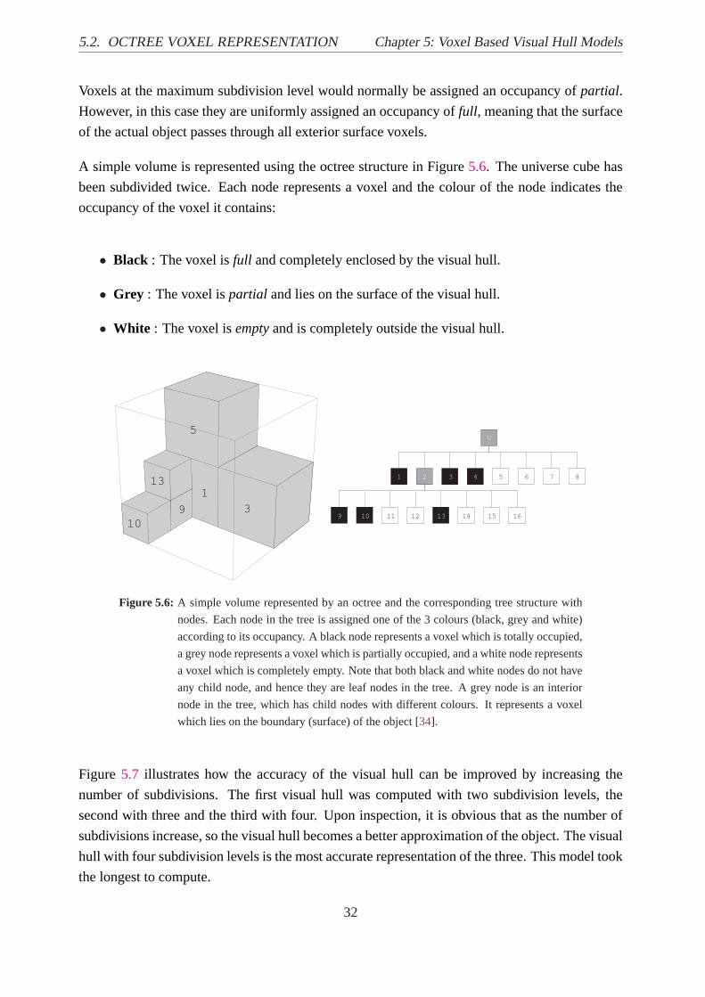
5.2 Octree Voxel Representation. . . . . . . . . . . . . . . . . . . . . . . . . . . .31
5.2.1 Data Compression. . . . . . . . . . . . . . . . . . . . . . . . . . . . .33
6 Surface Approximation using Marching Cubes 35
6.1 Marching Squares. . . . . . . . . . . . . . . . . . . . . . . . . . . . . . . . . .35
6.1.1 2D Ambiguities. . . . . . . . . . . . . . . . . . . . . . . . . . . . . . .38
x

CONTENTS CONTENTS
6.2 Marching Cubes. . . . . . . . . . . . . . . . . . . . . . . . . . . . . . . . . . .38
6.2.1 Approximating the Surface. . . . . . . . . . . . . . . . . . . . . . . . . 39
6.2.2 3D Ambiguities. . . . . . . . . . . . . . . . . . . . . . . . . . . . . . .41
6.2.3 Marching Cubes applied to an Octree Model. . . . . . . . . . . . . . . 44
7 Improving the Surface Estimate 47
7.1 A Binary Search in 2D. . . . . . . . . . . . . . . . . . . . . . . . . . . . . . .47
7.2 Searching along the Voxel Edge. . . . . . . . . . . . . . . . . . . . . . . . . . 49
8 System Overview 51
8.1 Image Acquisition. . . . . . . . . . . . . . . . . . . . . . . . . . . . . . . . . .51
8.1.1 System Calibration. . . . . . . . . . . . . . . . . . . . . . . . . . . . .51
8.1.2 Image Segmentation. . . . . . . . . . . . . . . . . . . . . . . . . . . .52
8.1.3 Estimation of the Universe Cube. . . . . . . . . . . . . . . . . . . . . . 52
8.2 The Final Algorithm . . . . . . . . . . . . . . . . . . . . . . . . . . . . . . . .52
8.2.1 Voxel Generation Algorithm. . . . . . . . . . . . . . . . . . . . . . . . 53
8.2.2 Marching Cubes Algorithm. . . . . . . . . . . . . . . . . . . . . . . . 53
8.2.3 Vertex Binary Search Algorithm. . . . . . . . . . . . . . . . . . . . . . 54
8.3 Computing Visual Hull Volumes. . . . . . . . . . . . . . . . . . . . . . . . . . 55
8.3.1 Voxel Model Volume Computation. . . . . . . . . . . . . . . . . . . . . 55
8.3.2 Marching Cube Model Volume Computation. . . . . . . . . . . . . . . 55
8.4 Website Tutorial. . . . . . . . . . . . . . . . . . . . . . . . . . . . . . . . . . .56
9 Experimental Results 67
9.1 Test Data Set. . . . . . . . . . . . . . . . . . . . . . . . . . . . . . . . . . . .67
xi

CONTENTS CONTENTS
9.2 Error Comparisons. . . . . . . . . . . . . . . . . . . . . . . . . . . . . . . . .68
9.2.1 Confidence Intervals. . . . . . . . . . . . . . . . . . . . . . . . . . . .71
9.3 Time Comparisons. . . . . . . . . . . . . . . . . . . . . . . . . . . . . . . . .76
9.4 Number of Elements. . . . . . . . . . . . . . . . . . . . . . . . . . . . . . . .76
10 Conclusions 79
10.1 Limitations . . . . . . . . . . . . . . . . . . . . . . . . . . . . . . . . . . . . .80
10.2 Scope for Further Investigation. . . . . . . . . . . . . . . . . . . . . . . . . . . 80
A Chernyaev’s MC33 Marching Cube Surfaces 81
B Lookup Table for the MC33 Cube Categories 83
xii

List of Figures
3.1 20 Faced Calibration Object.. . . . . . . . . . . . . . . . . . . . . . . . . . . .12
3.2 The Pinhole Camera Model.. . . . . . . . . . . . . . . . . . . . . . . . . . . .13
3.3 Multiple Camera System.. . . . . . . . . . . . . . . . . . . . . . . . . . . . . .15
3.4 Mirror Camera System.. . . . . . . . . . . . . . . . . . . . . . . . . . . . . . .16
3.5 Rotating Camera System.. . . . . . . . . . . . . . . . . . . . . . . . . . . . . .17
4.1 A Grey-Scale Image and Associated Silhouette Image.. . . . . . . . . . . . . . 20
4.2 Threshold Segmentation.. . . . . . . . . . . . . . . . . . . . . . . . . . . . . .21
4.3 Single Visual Cone.. . . . . . . . . . . . . . . . . . . . . . . . . . . . . . . . .23
4.4 Intersecting Visual Cones.. . . . . . . . . . . . . . . . . . . . . . . . . . . . .24
4.5 Effect of Increasing the Number of Views.. . . . . . . . . . . . . . . . . . . . . 25
5.1 2D Voxelised Image of a Cat.. . . . . . . . . . . . . . . . . . . . . . . . . . . .28
5.2 Cuberille Grid. . . . . . . . . . . . . . . . . . . . . . . . . . . . . . . . . . . .28
5.3 Indexed Voxel Vertices.. . . . . . . . . . . . . . . . . . . . . . . . . . . . . . .29
5.4 Voxel Occupancy Computations.. . . . . . . . . . . . . . . . . . . . . . . . . . 30
5.5 Incorrect Voxel Occupancy Computation.. . . . . . . . . . . . . . . . . . . . . 31
5.6 Octree Structure.. . . . . . . . . . . . . . . . . . . . . . . . . . . . . . . . . .32
xiii

LIST OF FIGURES LIST OF FIGURES
5.7 Three Voxel-Based Visual Hull Models of a Cat.. . . . . . . . . . . . . . . . . . 33
6.1 Sampledf (x) = sin(x). . . . . . . . . . . . . . . . . . . . . . . . . . . . . . . .36
6.2 The Marching Squares Look-up Table.. . . . . . . . . . . . . . . . . . . . . . . 37
6.3 Marching Squares applied to the Image of a Cat.. . . . . . . . . . . . . . . . . . 38
6.4 Ambiguous Marching Squares.. . . . . . . . . . . . . . . . . . . . . . . . . . . 39
6.5 Complementary Symmetry of a Voxel.. . . . . . . . . . . . . . . . . . . . . . . 40
6.6 Rotational Symmetry of a Voxel.. . . . . . . . . . . . . . . . . . . . . . . . . . 41
6.7 The MC15 Marching Cube Surfaces.. . . . . . . . . . . . . . . . . . . . . . . . 42
6.8 Ambiguities in the Cat’s Surface. . . . . . . . . . . . . . . . . . . . . . . . . . 43
6.9 Cause of Marching Cubes Inconsistencies. . . . . . . . . . . . . . . . . . . . . 43
6.10 Labelling System used for Voxel Edges and Faces.. . . . . . . . . . . . . . . . 44
6.11 Three MC33 visual hull Models of a Cat.. . . . . . . . . . . . . . . . . . . . . 44
7.1 1D Binary Search.. . . . . . . . . . . . . . . . . . . . . . . . . . . . . . . . . .47
7.2 Two Iterations of the Binary Search Applied to a 2D Intersection.. . . . . . . . . 48
7.3 2D Binary Search Applied to Marching Squares Output.. . . . . . . . . . . . . 49
7.4 Three Marching Cubes Visual Hull Surfaces of a Cat using a Binary Search.. . . 50
8.1 Five Camera System with Projected Cones.. . . . . . . . . . . . . . . . . . . . 57
8.2 Five Images Generated using Camera System.. . . . . . . . . . . . . . . . . . . 58
8.3 Voxel Reconstruction Algorithm Flow Chart.. . . . . . . . . . . . . . . . . . . 59
8.4 Six Rotated Views of a Voxel Based Visual Hull.. . . . . . . . . . . . . . . . . 60
8.5 Marching Cubes Visual Hull Construction Algorithm Flow Chart.. . . . . . . . 61
8.6 Six Rotated Views of a Marching Cubes Visual Hull.. . . . . . . . . . . . . . . 62
xiv

LIST OF FIGURES LIST OF FIGURES
8.7 Vertex Binary Search Algorithm Flow Chart.. . . . . . . . . . . . . . . . . . . 63
8.8 Six Rotated Views of a Marching Cubes Visual Hull with Binary Search.. . . . . 64
8.9 Visual Hull of a Cat Computed from the Different Methods.. . . . . . . . . . . 65
9.1 Graph of RMS Percentage Errors.. . . . . . . . . . . . . . . . . . . . . . . . . 70
9.2 Graph 95% Confidence Intervals for Resolution 1.. . . . . . . . . . . . . . . . . 72
9.3 Graph 95% Confidence Intervals for Resolution 2.. . . . . . . . . . . . . . . . . 73
9.4 Graph 95% Confidence Intervals for Resolution 3.. . . . . . . . . . . . . . . . . 74
9.5 Graph 95% Confidence Intervals for Resolution 4.. . . . . . . . . . . . . . . . . 75
9.6 Graph 95% Confidence Intervals for Resolution 5.. . . . . . . . . . . . . . . . . 75
A.1 Chernyaev’s MC33 Marching Cubes Surfaces.. . . . . . . . . . . . . . . . . . . 82
xv

LIST OF FIGURES LIST OF FIGURES
xvi
List of Tables
9.1 Percentage RMS Error Comparisons forVm. . . . . . . . . . . . . . . . . . . . . 69
9.2 Percentage Absolute Error Comparisons forVm. . . . . . . . . . . . . . . . . . . 69
9.3 Percentage RMS Error Comparisons forVest. . . . . . . . . . . . . . . . . . . . 69
9.4 Percentage Absolute Error Comparisons forVest. . . . . . . . . . . . . . . . . . 70
9.5 Difference in Percentage RMS Error Values forVest at Varying Resolutions.. . . 70
9.6 Difference in Percentage RMS Error Values forVest using the Different Methods. 71
9.7 Resolution 1 Confidence Interval forVest. . . . . . . . . . . . . . . . . . . . . . 72
9.8 Resolution 2 Confidence Interval forVest. . . . . . . . . . . . . . . . . . . . . . 73
9.9 Resolution 3 Confidence Interval forVest. . . . . . . . . . . . . . . . . . . . . . 73
9.10 Resolution 4 Confidence Interval forVest. . . . . . . . . . . . . . . . . . . . . . 74
9.11 Resolution 5 Confidence Interval forVest. . . . . . . . . . . . . . . . . . . . . . 74
9.12 Speed Comparisons for Voxels vs Marching Cubes.. . . . . . . . . . . . . . . . 76
9.13 Speed Comparisons as Resolution is Increased.. . . . . . . . . . . . . . . . . . 77
9.14 Percentage Increase in Speed from Voxels to Marching Cubes.. . . . . . . . . . 77
9.15 Percentage Increase in Speed for Binary Search.. . . . . . . . . . . . . . . . . . 77
9.16 Average Number of Elements for Voxels vs Marching Cubes at various Subdivi-
sion Levels. . . . . . . . . . . . . . . . . . . . . . . . . . . . . . . . . . . . . .78
xvii

LIST OF TABLES LIST OF TABLES
B.1 MC33 Test Table.. . . . . . . . . . . . . . . . . . . . . . . . . . . . . . . . . .84
xviii

Glossary
2D—Abbreviation oftwo dimensional. Has a coordinate system consisting of two orthogonal
axes(x,y).
3D—Abbreviation ofthree dimensional. Has a coordinate system made up of three orthogonal
axes(x,y,z).
Camera Calibration—The process that sets numerical values for the extrinsic and intrinsic
parameters of a camera and/or the external 3D position and orientation of a camera frame relative
to an external coordinate system [4].
Extrinsic camera parameters—External camera parameters. Describes the location and orien-
tation of the camera with respect to the world coordinate system.
Intrinsic camera parameters—Internal camera parameters. Describes the total magnification
of the imaging system resulting from both optics and image sampling as well as the principal
point.
Grey-Scale Image—An intensity image. Pixels are represented by a single value that ranges
from 0 (black) to 1 (white).
MATLAB— A high-performance programming language for technical computing.
MEX— Abbreviation ofMATLAB executable.
Morphological Operators—Morphological operators are applied to binary images. They can
be used to smooth or even extract edges. Basic operators include erosion, dilation, opening and
closing.
Pixel—Abbreviation ofpicture element. It is the smallest element of a 2D image.
RGB Image—Abbreviation ofred, green and blue image. Synonym for “colour image”. Each
pixel has separate values for red, green and blue.
xix

LIST OF TABLES LIST OF TABLES
RMS—Abbreviation ofroot mean square.
Segmentation—The process of separating an image into foreground (or target) and background
regions.
Silhouette Image—An image that contains the silhouette of an object. Formed through the
segmentation of a grey-scale or RGB image.
Topology—Branch of mathematics concerned with generalisation of concepts of continuity, limit
etc.
Visual Cone—A cone-like volume that is formed by the projection of a silhouette from the
camera centre.
Visual Hull— The closest approximation to an object that can be obtained with the volume inter-
section approach. The visual hull is the largest object that can be substituted for the actual object
and still result in the same finite set of silhouettes.
Voxel—Abbreviation ofvolume element. A voxel is a cube.
xx

Chapter 1
Introduction
The ability to accurately model real world objects in computer graphics and machine vision is
an extremely powerful tool. Structural information contained in a 3D model is of great value in
a wide range of systems: Computer games and animations often use objects from the real world;
gesture recognition is simplified with a detailed knowledge of the shape of a person’s limbs;
shape classification systems require structural information of an object; geologists often require
the size and shape distributions for a batch of rocks in various scientific evaluations.
Due to the demand from so many fields, a large amount of work has been done on modelling 3D
objects. Previously, mostly offline systems were used. Optical systems, based on the acquisition
of images that contain the object, can be separated intoactive and passivesystems. Active
systems, such as expensive laser scanners, cast a structured light over the object. Passive systems
obtain information from the analysis of images that contain the object. Some passive systems are
marker based, requiring undesirable invasive markers to be placed on an object. The silhouette-
based approach has many advantages:
• It is relatively inexpensive.
• Cameras are easy to configure.
• It is non-invasive, as it does not require a marker system.
• Images contain both shape and texture information of a target object.
Structural information of an object is contained in any 2D image of that object. From a single
view of an object, it is possible to make certain estimates about the dimensions of the object
as well as its position relative to the camera. An estimate is improved with an increase in the
1

1.1. OBJECTIVES OF THIS THESIS Chapter 1: Introduction
number of sufficiently different views available. The information from each camera needs to be
coordinated so that precise 3D measurements can be inferred.
Over a number of years, many different methods for representing 3D models have been devel-
oped, some more efficient than others. Thevisual hullof an object is generally accepted as an
adequate representation[14] and hence, the volume of the visual hull is a good approximation to
the actual volume of the object.
Voxel-based methodsuse a number of small cubes (or 3D pixels) to construct the visual hull.
Although the resultant models are extremely accurate at higher resolutions, they are compu-
tationally expensive. The surface of a voxel-based model is made up of a number of cubes,
causing the model’s surface to appear jagged. A representation consisting of polygons would
provide smoother and easier to manipulate visual hull models.
One solution to this problem is to build a coarse voxel model and then apply an algorithm known
asmarching cubes, which replaces surface cubes with polygons. With minimal effect on the
computational time required, this algorithm can drastically improve the accuracy of the model.
1.1 Objectives of this Thesis
Many systems use the volume distribution of rock samples as an input to control a process.
Manual volume measurements for a large set of rocks are tedious. Computing the volume from
the visual hull of a rock is a fast and automated process.
The objective of this thesis is to implement a system that can quickly compute the volume of an
object from its visual hull using multiple views of the object. A target object’s visual hull will
be calculated from silhouette images, obtained in an accurately calibrated camera system. The
visual hull will be described in three stages:
• Voxel Based Models- A 3D space is partitioned into cubic volume elements (orvoxels)
and a binary marking system is used to represent the visual hull’s basic structure.
• Marching Cube Models - The marching cubes algorithm assigns triangular patches to
surface voxels of the voxel-based visual hull.
• Modified Marching Cube Models - The positional accuracy of each triangle corner cre-
ated with the marching cubes algorithm is improved by applying a binary search.
The system’s performance will be quantified at the three stages of the algorithm by comparing
2

Chapter 1: Introduction 1.2. THESIS OUTLINE
the amount of time required to complete the visual hull computation and the RMS percentage
volume errors.
1.2 Thesis Outline
This thesis discusses the theory needed to build the visual hull of an object using silhouette
projection methods for volume estimation. An algorithm is developed and tested at three stages
on a data set of stones. The following is a brief summary of the remaining chapters.
Chapter 2 contains a literature review that gives a background to the theoretical ideas involved
in the implementation of this project. Valuable sources of information on camera geometry and
methods used for volume computation are summarised. Practical applications for automated vol-
ume estimators are examined and work done in the field of “shape from silhouettes” is contained
in this chapter. Various methods for representing the visual hull of an object are introduced.
Chapter 3 describes the camera system used to obtain images, as well as the way that 3D mea-
surements are obtained from 2D images. The pinhole camera model is described and the three
coordinate systems that it defines are listed. Various environments that accommodate for the
capture of multiple views of an object are investigated.
Chapter 4 discusses the concept of “volume intersection”, which is used to obtain the visual hull
of an object from an accurately calibrated camera environment. The segmentation of images and
the projection of silhouettes into a 3D space are also covered.
Chapter 5 describes the ideas associated with voxel-based visual hulls. A volume is partitioned
into small cubic cells and each cell’s value is set so that the volume represents the visual hull of
an object. This chapter makes use of 2D analogies to explain some of the key ideas.
In chapter 6, the marching cubes algorithm is explained. The marching cubes algorithm ap-
proximates the intersection of a surface through a cube by tiling it with triangular patches. 2D
analogies are used to illustrate the effects of the algorithm.
An extension to the marching cubes algorithm is introduced in chapter 7. The extension applies
single iterations of a binary search to the vertices of each surface patch, resulting in a better visual
hull approximation of the object. A 2D analogy of this algorithm simplifies its description.
Details on the algorithms used to implement the voxel-based, marching cubes and binary search
visual hulls are provided in chapter 8. An accurately calibrated camera system captures multiple
views of a target object. Captured images are segmented to form silhouettes that are extruded
3

1.2. THESIS OUTLINE Chapter 1: Introduction
and used to compute the visual hull model using voxel-based methods. The marching cubes
algorithm is applied to the voxel model, replacing surface voxels with triangular patches. This
has the effect of smoothing the visual hull surface. A binary search is used to further refine the
accuracy of the visual hull. Techniques that are used to compute the volume of voxel based and
marching cube models are described in this chapter.
Chapter 9 presents the testing methods and discusses the results obtained from these tests. This
chapter contains a performance comparison between the three stages of the algorithm. A data set
of stones that represent a wide distribution of naturally occurring shapes is used to test the via-
bility of the system. Accuracy and speed improvements resulting from the voxel model and the
marching cubes algorithm, both with and without the binary search, are be evaluated. A method’s
accuracy is measured using RMS percentage error statistics, which are computed through a com-
parison of computed visual hull volumes with ground truth values. The increase or decrease in
processing time required is also studied.
Finally, chapter 10 presents conclusions, limitations and proposes scope for future research. The
link to a website containing a tutorial on the algorithms, as well as working code, is also pro-
vided.
4

Chapter 2
Literature Review
This chapter provides a description of work already done in the various fields discussed in later
chapters. Each source of information contains valuable insight on ideas and concepts, which
results in the implementation of a working algorithm that can accurately and quickly compute
the volume of an object from multiple image views.
Volume estimation systems are outlined in section 2.1. The sections that follow briefly describe
work already done on the subject of visual hull reconstructions. Section 2.3 looks at the methods
used to compute the volume of a visual hull.
2.1 Background
The size and shape distribution for a batch of stones has a major role to play in the strength,
stability and performance of concrete and asphalt. Manual systems use sampling techniques
to monitor the distribution of particles. This method is time consuming and makes real-time
feedback for control purposes impossible.
A 3D-laser scanning technique is used by Lanaroet al. [11] to evaluate coarse-grain aggregate-
particle images. They are able to achieve reliable results for both the shape and topographical
parameters of particles. The laser sensor used in experiments is sensitive to environmental con-
ditions, making it more suited to laboratory investigations.
2D images are used by Bantaaet al. [12] to determine the distribution of particle sizes in asphalt
pavements. They estimate the size and shape characteristics of multiple stones from a single
segmented view. The single view means that stereo information is not available and therefore,
an average value for height is used when computing particle volumes. In their system, exact
5

2.2. SHAPE FROM SILHOUETTE Chapter 2: Literature Review
volume measurements for a single particle are not critical. Raoet al. [28] use three camera
views, which provide them access to vital stereo information. Particles are individually sent
through their system, providing better estimates at slower speeds. Cameras are positioned in a
way that allows them to capture orthogonal views of a particle, resulting in the calculation of
more accurate volume estimations. Their system is used to automate the determination of flat
and elongated particles, angularity, and gradation.
2.2 Shape from Silhouette
In many applications it is intrusive or impractical to attach foreign marker objects to the body of
the subject. Non-intrusive techniques are therefore more desirable.
A human observer can, in most cases, recognise an object from the shape of its silhouette. The
silhouette of a 3D object is therefore a valid source of shape information. The concept of using
silhouettes for 3D shape reconstruction was first introduced by Baumgart in 1974. In Baumgart’s
PhD thesis [3], four silhouette images are used to estimate the 3D shape of a baby doll and a
toy horse. Silhouette images are the result of segmenting a grey-scale or RGB image intotarget
andbackgroundregions. Segmentation is a widely researched branch of image processing and
is available in many forms, such as region growing, contour modelling and thresholding.
Hamblinet al. [10] show that there is a relationship between the complexity of a particle and the
sensitivity to the positioning of viewing points. The more uniformly a particle’s dimensions vary
through different planes, the less a viewing technique affects its approximations.
Olssonet al. [26] uses a single stationery camera to capture views about a rotating object. The
use of a single camera, instead of multiple cameras, makes their method more cost effective,
while the rotating object enables them to retain the ability to capture multiple views.
Pollefeys [27] presents a technique that can obtain realistic 3D models of existing monuments
from a few old photographs. The flexibility of his technique allows it to be used on video ma-
terial. His algorithm is minimally dependant on calibration information and therefore, produces
scale invariant models.
2.2.1 Camera Geometry
Camera calibration is a widely studied research topic in computer vision. Before computer vi-
sion, it was extensively investigated in the field of photogrammetry. Calibration is a necessary
6

Chapter 2: Literature Review 2.2. SHAPE FROM SILHOUETTE
step in inferring 3D measurements from 2D images [19].
Chavarriagaet al. [4] provides an in-depth description of the camera model, as well as valuable
mathematical detail on the calibration process.
Various methods have been developed to determine the pose corresponding to each camera in a
multi-camera system. Tsai [33] has developed an autonomous technique for camera calibration
using standard off-the-shelf cameras. Tsai’s method uses an advanced bar coded pattern printed
on a calibration object. The calibration object is required to be a fixed distance from the camera.
2.2.2 The Visual Hull
The termvisual hullwas formally defined in 1991 by Laurentini [13]. For more than a decade
before this, it had been used in a general sense by researchers. Laurentini defines the visual hull
as the entity used to describe the largest object consistent withall possiblesilhouettes. However,
the term is usually used to refer to the largest object that is consistent with afinite set of available
silhouettes. The visual hull is known to include the object and to be included in the object’s
convex hull [14].
Shakhnarovichet al. [29] describes a system that uses four, evenly spaced, fixed cameras at
approximately the same height. Using visual hull reconstructions, they are able to recognise a
person from a combination of facial features and gait.
Cheung [6] uses a single camera to capture multiple view silhouettes of a moving subject. Using
a model of the human body, a coarse visual hull of the subjects is initially computed. As time
progressed, and more silhouette information became available, the accuracy of the visual hull
model improves.
Niem et al. [25] use a single camera and a turntable to obtain multiple silhouette images of an
object at different viewpoints. The relative poses of the turntable platform with respect to the
camera are determined with the aid of a calibration object. They computed the visual hull model
with volume carving techniques and generated a triangular mesh to represent its surface.
A newer method, implemented by Matusiket al. [21] makes use of polygons to represent the vi-
sual hull. They developed an algorithm that reduces 3D intersections to simpler 2D intersections.
Their algorithm produces view-independent representations that are computed very quickly. The
visual hull is formed by its polygonal faces, each of which lie on a face of one of the visual
cones. The visual hull faces are therefore formed by the intersection of the faces of each visual
cone with all remaining visual cones.
7

2.2. SHAPE FROM SILHOUETTE Chapter 2: Literature Review
2.2.3 Voxels and the Octree Model
Volume intersection techniques for constructing a volumetric description of an object from mul-
tiple views, was first proposed in 1983 by Martin and Aggarwal [20]. Ahuja and Veenstra [1]
presented an extension to this technique, which generated an octree to represent an object from
any subset of 13 standard viewing directions.
The main thrust of Small’s MSc thesis [30] is to be able to compute the visual hull in real-
time. Binary volumetric images are used to represent the visual hull model. Small’s review of
calibration techniques and volume intersection gives useful insight on the subjects.
2.2.4 Marching Cubes
In 1987, Lorensen and Cline [18] present an algorithm that creates a triangular mesh for medical
data. Known as “marching cubes” due to the way it “marches” from one element to the next,
the algorithm is considered to be the basic method for surface rendering in medical applications.
In this text their original algorithm will be referred to as MC15. They use MC15 to process
2D computer tomography slices in scan line order, while maintaining inter-slice connectivity. A
lookup table, containing 15 possible surface intersections allows the MC15 algorithm to be fast.
MC15 can be applied in other areas, as for example, in the visualisation of implicitly specified
functions or even the visualisation of calculation results. They also note that the generated surface
contains a large number of triangles.
Nielsonet al. [24] found that MC15 has no topological guarantees for consistency and produces
visual hull surfaces containing small holes or cracks due to certain voxel face ambiguities. Using
definitions ofseparatedandnon-separatedvoxel vertices, they are able to propose a modification
to MC15 that implements face tests to resolve the ambiguities. They do not guarantee the correct
topology either, and propose an internal test to resolve other ambiguities. In 1995, Chernyaev [5]
showed that there are 33 topologically different surface intersections and not 15. His algorithm
will be referred to as MC33. Chernyaev found ambiguous cases that are not visibly obvious and
uses the suggested internal tests to resolve the remaining ambiguous voxel arrangements.
Montaniet al. [23] noted the topological inconsistency, computational efficiency and excessive
data fragmentation as disadvantages of MC15. They propose a method to minimise the number
of triangular patches specified in the marching cubes surface lookup table, reducing the amount
of data output and improving the computational efficiency. The test table which they use to
resolve ambiguous voxel configurations is shown in figureA.1 of the appendices.
In a paper by Lewineret al. [16], an efficient and robust implementation of Chernyaev’s MC33
8

Chapter 2: Literature Review 2.3. VISUAL HULL VOLUMES
algorithm is described. Detailed information, covering lookup tables, voxel labelling systems
and tests to resolve voxel ambiguities, is provided. Their system guarantees a consistent surface
without holes or cracks.
Tarini et al. [31] developed a fast and efficient version of the marching cubes algorithm, called
marching intersections, to implement a volumetric based visual hull extraction technique. Using
a large 3D mesh configuration, scans of the target are made. The point at which the ray intersects
with the target is stored. The paper also provides a good definition of the visual hull computed
from images captured with a turntable.
In Wong’s PhD thesis [34], a detailed description of the entire visual hull computation process
can be found. Wong describes the static properties of silhouettes and then studies the dynamic
properties of a moving camera system. He uses an octree system to represent the visual hull,
and then applies the marching cubes algorithm, which allows the constructed 3D model to be
displayed efficiently in conventional graphics rendering systems.
2.3 Visual Hull Volumes
Part of the objective of this thesis is to compute the volume for a given visual hull. To compute
the volume of an voxel based model is as simple as summing the volume of a list of cubes.
The volume enclosed by a polygon model can be calculated in a number of ways. The method
used is summarised in section 2.3.1. It was not necessary to find alternate volume computation
techniques as this method was deemed adequate.
2.3.1 Volume Computation for Polyhedra
A marching cube surface consists of a list of polygonal surfaces, that are stitched together to
form the visual hull of an object. Many methods for calculating the volume, mass or moment
of inertia of polyhedra are computationally expensive or produce approximate results. Lien and
Kajiya [17] developed a technique that not only produces an exact solution, but is also efficient.
They integrate a set of tetrahedra formed by each triangular face and the origin. Their method
also allows for the computation of the visual hull’s centroid.
9

2.3. VISUAL HULL VOLUMES Chapter 2: Literature Review
10

Chapter 3
Camera System
When taking 3D measurements from 2D images, knowledge of the intrinsic and extrinsic param-
eters of the camera is crucial. In a multi-camera environment, the relative poses and positioning
of each camera is also of great importance. This criteria requires that the camera system involved
be accurately calibrated. A number of environments that enable the capture of multiple views of
an object are also introduced in this chapter.
3.1 Calibration Process
Calibration is the process that enables the setting of numerical values for the geometrical and
optical (intrinsic and extrinsic) parameters of the camera and/or the external 3D position and
orientation of the camera frame relative to an external coordinate system [4]. The output of this
process is normally a pose transformation matrix, which is a4× 4 matrix that applies arigid
body transformto a set of points. A rigid body transform performs a rotation and a translation
on a set of points, while preserving the lengths and angles between the points.
System calibration can be done in many ways. One of the more commonly used methods in-
volves the use of a calibration object. Once calibrated, each camera is associated with apose
transformation matrixthat enables a transformation from the camera’s own reference frame to a
world coordinate system that encompasses the entire system [9].
A calibration object can be of any size or proportion (preferably matched to the camera’s field
of view), as long as its dimensions are accurately known. An example of a 20-sided calibration
object is shown in Figure3.1. This object was constructed from cardboard. Each of the trian-
gular faces is marked with a binary labelling system. Using an object of this type enables an
11

3.1. CALIBRATION PROCESS Chapter 3: Camera System
uncalibrated system to calculate the exact orientation of the object with respect to each camera’s
reference frame. Once all of these orientations have been computed, each camera’s pose and
position in the system can be calculated [8].
Figure 3.1: The 20 faced calibration object constructed from cardboard. Each face is marked with
a unique binary coded pattern.
Most cameras perform a perspective transformation on points in a 3D space to 2D points in the
retinal (or image) plane. The geometry of 2D images was first studied by Italian artists during
the Renaissance so that they could reproduce objects from the real world more accurately [7].
Although real cameras have apertures of finite size and use lenses for focussing light onto the
retinal plane,the pinhole camera modelis an excellent approximation of the imaging process [9].
3.1.1 Pinhole Camera Model
This perspective projection model, illustrated in Figure3.2, assumes that light enters the camera
through a dimensionless point (or pinhole) at the camera centre and projects onto the retinal
plane.
The camera centre, also called thefocal point, is situated between the object and retinal plane.
The imaged object appears inverted in the retinal plane due to light rays travelling through the
optical centre and onto the retinal plane. Positioning the retinal plane in front of the camera, as
in Figure3.2(b), is geometrically equivalent and sometimes seen as being more intuitive [32].
The pinhole camera model defines animage coordinate systemand acamera coordinate system.
In a multi-camera system, aworld coordinate systemis also defined so that camera positions are
12

Chapter 3: Camera System 3.1. CALIBRATION PROCESS
C
Camera coordinate
system
Image coordinate
system
Opticalaxis
(U ,v )0 0
f
Opticalray
Object
m
m’
XZ
Y
World coordinate
system
xZ
Y
R
X
Y
(a)
Opticalaxis
C
(u ,v )0 0
Image coordinate
system
Camera coordinate
system
Object
m
m’
XZ
Y
R f
Opticalray
World coordinate
system
xZ
Y
X
Y
(b)
Figure 3.2: In the pinhole camera model, the retinal plane (ℜ) and the camera centre (a pointC
that does not belong toℜ) are shown.C is the focal point. The distance from the focal
point to the centre of the retinal plane is the focal length,f . The scene point,m, on
an object, is mapped to the pointm′ in the retinal plane. A right-handed coordinate
system is employed. The imaged object is inverted in illustration (a). The model in
(a) is geometrically equivalent to the model shown in (b), where the retinal plane is
situated between the camera centre and the imaged object.
13

3.1. CALIBRATION PROCESS Chapter 3: Camera System
known relative to each other.
Affine Image Coordinate System
Most images use pixels as their unit of measurement, but this is dependent on the technology of
the camera. Images use a 2D coordinate system that generally has its origin positioned in the top
left corner of the image. The point that is directly in front of the camera, situated in the retinal
plane, is known as the principal point and has coordinates(u0,v0). This point is near the centre
of the image.
Euclidean Camera Coordinate System
In the camera’s 3D coordinate system, the camera is positioned at the optical centre (0,0,0).
The focal length (f ) is the distance from the optical centre along the optical axis to the point of
intersection with the retinal plane. This point of intersection, known as the principal point (which
is near the image centre), is situated at(0,0, f ). Camera coordinates are generally measured in
metres or millimetres.
World Coordinate System
The world coordinate system is introduced to link together all the camera systems available. It is
used to describe the location and orientation of each camera with respect to the others.
Retinal Plane to Camera Reference Frame
To map a point in the retinal plane to a point in camera coordinates, the units need to be converted
to match that of the cameras. The retinal plane is a distancef from the optical centre, making the
z coordinate of any point in the image equal tof . Thex andy coordinates of the image need to
be translated byu0 andv0 respectively, as the principal point in image coordinates is at(u0,v0)and(0,0, f ) in the camera’s coordinate system.
14

Chapter 3: Camera System 3.2. MULTI-VIEW CAMERA SYSTEMS
3.2 Multi-view Camera Systems
Multiple image views can be obtained from a variety of different camera systems. The visual
hull becomes a closer approximation of the object with an increase in the number of significantly
different available views. Three different camera arrangements for generating multiple views of
an object follow. Optimum positioning of the cameras is a subject that is not covered.
3.2.1 Multiple Camera Environment
Multiple cameras are arranged about the object. A multi-camera arrangement is the most intuitive
as well as the simplest of the three to implement. Due to the use of more cameras, it is also the
most expensive. Figure3.3 shows a 2D illustration of this type of camera arrangement using
only two cameras. Since the intrinsic parameters of each camera may vary, each camera has to
be separately calibrated.
aaaaaaaaaaaaaaaaaaaaaaaaaaaaaaaaaaaaaaaaaaaaaaaaaaaaaaaaaaaaaaaaaaaaaaaaaaaaaaaaaaaaaaaaaaaaaaaaaaaaaaaaaaaaaaaaaaaaaaaaaaaaaaaaaaaaaaaaaaaaaaaaaaaaaaaaaaaaaaaaaaaaaaaaaaaaaaaaaaaaaaaaaaaaaaaaaaaaaaaaaaaaaaaaaaaaaaaaaaaaaaaaaaaaaaaaaaaaaaaaaaaaaaaaaaaaaaaaaaaaaaaaaaaaaaaaaaaaaaaaaaaaaaaaaaaaaaaaaaaaaaaaaaaaaaaaaaaaaaaaaaaaaaaaaaaaaaaaaaaaaaaaaaaaaaaaaaaaaaaaaaaaaaaaaaaaaaaaaaaaaaaaaaaaaaaaaaaaaaaaaaaaaaaaaaaaaaaaaaaaaaaaaaaaaaaaaaaaaaaaaaaaaaaaaaaaaaaaaaaaaa
Object
Hull
Camera
Camera
Figure 3.3: Two cameras are used to view a blacktargetobject. The textured grey section repre-
sents the resultant hull.
3.2.2 Mirror and Camera Environment
Mirrors can be used to reduce the number of expensive cameras required in the implementation.
Multiple views of the object are provided by mirrored reflections of the object (see Figure3.4).
This increases the mathematical complexity of the system. An advantage of this arrangement is
15

3.2. MULTI-VIEW CAMERA SYSTEMS Chapter 3: Camera System
that the addition of extra mirrors, rather than expensive cameras, makes more views of the object
available. A possible negative aspect is that the use of mirrors results in a decrease in clarity
of the reflected object due to the object appearing smaller in the reflected camera view than the
direct camera view.
aaaaaaaaaaaaaaaaaaaaaaaaaaaaaaaaaaaaaaaaaaaaaaaaaaaaaaaaaaaaaaaaaaaaaaaaaaaaaaaaaaaaaaaaaaaaaaaaaaaaaaaaaaaaaaaaaaaaaaaaaaaaaaaaaaaaaaaaaaaaaaaaaaaaaaaaaaaaaaaaaaaaaaaaaaaaaaaaaaaaaaaaaaaaaaaaaaaaaaaaaaaaaaaaaaaaaaaaaaaaaaaaaaaaaaaaaaaaaaaaaaaaaaaaaaaaaaaaaaaaaaaaaaaaaaaaaaaaaaaaaaaaaaaaaaaaaaaaaaaaaaaaaaaaaaaaaaaaaaaaaaaaaaaaaaaaaaaaaaaaaaaaaaaaaaaaaaaaaaaaaaaaaaaaaaaaaaaaaaaaaaaaaaaaaaaaaaaaaaaaaaaaaaaaaaaaaaaaaaaaaaaaaaaaaaaaaaaaaaaaaaaaaaaaaaaaaaaaaaaaaaaaaaaaaaaaaaaaaaaaaaaaaaaaaaaaaaaaaaaaaaaaaaaaaaaaaaaaaaaaaaaaaaaaaaaaaaaaaaaaaaaaaaaaaaaaaaaaaaaaaaaaaaaaaaaaaaaaaaaaaaaaaaaa
Camera
Mirror
VirtualCamera
Hull
Object
Figure 3.4: A single camera is used to view a blacktargetobject. The mirror reflects the image of
the object creating a view from a virtual camera. The textured grey section represents
the resultant hull.
3.2.3 Rotating Camera or Object
Multiple views of an object can be obtained by rotating it with respect to the camera and capturing
images in sequence. A rotational system is not always practical in a real time environment, but is
ideal for offline situations. The simplest method involves placing an object on a rotating platform
that allows controlled increments through360◦. The accuracy of this system is dependent on the
number of rotational increments that the platform moves through, as well as the elevation of the
camera relative to the rotating platform. This system is equivalent to rotating a camera about a
stationary object as shown in Figure3.5.
16

Chapter 3: Camera System 3.2. MULTI-VIEW CAMERA SYSTEMS
aaaaaaaaaaaaaaaaaaaaaaaaaaaaaaaaaaaaaaaaaaaaaaaaaaaaaaaaaaaaaaaaaaaaaaaaaaaaaaaaaaaaaaaaaaaaaaaaaaaaaaaaaaaaaaaaaaaaaaaaaaaaaaaaaaaaaaaaaaaaaaaaaaaaaaaaaaaaaaaaaaaaaaaaaaaaaaaaaaaaaaaaaaaaaaaaaaaaaaaaaaaaaaaaaaaaaaaaaaaaaaaaaaaaaaaaaaaaaaaaaaaaaaaaaaaaaaaaaaaaaaaaaaaaaaaaaaaaaaaaaaaaaaaaaaaaaaaaaaaaaaaaaaaaaaaaaaaaaaaaaaaaaaaaaaaaaaaaaaaaaaaaaaaaaaaaaaaaaaaaaaaaaaaaaaaaaaaaaaaaaaaaaaaaaaaaaaaaaaaaaaaaaaaaaaaaaaaaaaaaaaaaaaaaaaaaaaaaaaaaaaaaaaaaaaaaaaaaaaaaaa
Hull
Object
Camera
RotatedCamera
Figure 3.5: A single camera is used to view a blacktarget object. The camera is rotated around
the object to obtain two views. The textured grey section represents the resultant hull.
17

3.2. MULTI-VIEW CAMERA SYSTEMS Chapter 3: Camera System
18
Chapter 4
The Visual Hull
Laurentini defines the visual hull of a 3D object as being “the closest approximation of S [an
object] that can be obtained with the volume intersection approach” [13]. The visual hull is the
largest volume that can be substituted for the actual object and still result in the same finite set
of silhouettes. Significant concavities, such as the inside of a tea cup, are not captured in visual
hull representations of an object.
The visual hull can be an exact copy of the object. It is never smaller than the object as it
always completely encloses the object. Compared to the convex hull, the visual hull is a closer
representation of a 3D object’s structure. Due to the visual hull being computed from an object’s
silhouette views, its shape is dependant on the shape of the object combined with the region of
the object viewed in the silhouettes.
This chapter begins with a description of the method used to compute an objects silhouette given
an image of the object. In the section that follows, volume intersection is investigated.
4.1 Silhouette Extraction
Identifying and reconstructing 3D objects based on 2D images has been under investigation for
a number of years. Even though silhouette-based approaches neglect surface features that could
be used to identify the object, they are still an excellent tool for object recognition.
The silhouette of any 2D image can be obtained through a process known as image segmentation.
This process is one of the most fundamental and important components in image processing. The
quality of an application is generally dependent on the accuracy of segmentation used, and hence
a good segmentation algorithm is extremely important [22]. Segmentation involves decomposing
19

4.1. SILHOUETTE EXTRACTION Chapter 4: The Visual Hull
an image into parts that are meaningful with respect to a particular application. In the visual hull
construction application, image regions are classified into the following two categories:
• Foreground(or Target)
• Background
Figure4.1 shows the segmentation of a grey-scale image of a small plastic cat intoforeground
andbackgroundregions. A silhouette image’s pixels have binary colour values that can be either
1 or 0, which indicate the pixel’s region classification.
(a) Grey-Scale Image (b) Segmented Image
Figure 4.1: The grey-scale image of a small plastic cat is shown in (a) and its associated silhouette
image in (b). Image (b) has been segmented into whiteforegroundand blackback-
groundregions.
There are a wide variety of segmentation algorithms available. Region growing, watersheds
and contour modelling [2] are among a few of the more intelligent algorithms that have been
developed. A less complex method places a simple threshold on an image’s intensity values.
Two dimensional images are made up of a number of small square picture elements calledpixels.
In grey-scale images, pixels store an intensity value that ranges between 0 and 255 or 0 and 1.
The threshold must lie within this range. Intensity values exceeding the threshold are classified as
foreground, while values below the threshold are classified asbackground. Figure4.2 illustrates
the concept of threshold segmentation. Using a threshold on an image provides adequate results
and also requires the least amount of processing time. It was for these reasons that thresholding
was used as the preferred segmentation technique.
20

Chapter 4: The Visual Hull 4.2. VOLUME INTERSECTION
13
13
13
14
14
13
14
15
15
14
15
55
14
55
13
14
56
55
58
13
13
13
57
57
13
(a)
0
0
0
0
0
1
0
1
0
0
1
1
1
0
0
0
0
0
0
0
0
1
1
00
(b)
Figure 4.2: This figure shows a grid of intensity values. In the first grid, a threshold of 50 has been
applied, and highlighted in white. The second grid shows how each value is labelled
asforeground(marked with ones) andbackground(marked with zeros).
Threshold segmentation, although relatively fast compared to other segmentation algorithms, can
result in grainy disconnected targets. Generally, better segmentation results are obtained through
the selection of an appropriate background, combined with controlled lighting. Morphological
operators are able to smooth out the grainy appearance of a target and improve the segmented
output.
4.2 Volume Intersection
Volume intersection, used in Laurentini’s definition of the visual hull, is described here. First,
computing the position of a 3D point is investigated, after which the idea is expanded to accom-
modate the intersection of a number of volume’s that form the visual hull.
4.2.1 Estimating the Position of a Point
Using a single image (i), the 3D position of a point (Mxyz) is constrained to lie somewhere along
the line projected from the camera centre (Ci0) through the imaged point (Mi) to infinity. The
equation of the line is given in equation4.1.
Mxyz= Ci0 +S∗ (Mi−Ci
0) (4.1)
21

4.2. VOLUME INTERSECTION Chapter 4: The Visual Hull
The variableSis an unknown scaling factor relating to the depth of the point. This value can only
be computed with the addition of a second view of the point, captured from a different location.
The point must lie at the intersection of the lines projected from each camera. However, due
to various inaccuracies inherent of the system, projected lines are not guaranteed to intersect.
For this reason the point is assumed to be positioned so that the perpendicular distance to each
projected line is minimised. Using equation4.2, we can solve forS.
b =
C1x −C2
x
C1y −C2
y
C1z −C2
z
(4.2a)
A =
M1x−C1
x M2x−C2
x
M1y−C1
y M2y−C2
y
M1z−C1
z M2z−C2
z
(4.2b)
S= A\b (4.2c)
Substituting this value into equation4.1gives us the 3D coordinates ofMxyz.
4.2.2 Visual Cone Projection
By the same principle used in the previous section, an object must lie within the cone-like volume
that is formed by an extrusion of its silhouette. A silhouette is extruded by projecting each point
in the silhouette from the camera centre through its location in the retinal plane. The volume
formed is known as avisual coneand it completely encloses the object (see Figure4.3).
With the addition of a different silhouette view of the object, the visual hull becomes a closer
representation of the object’s shape and location. Figure4.4shows two visual cones that intersect
to form the visual hull of an object. As the number of available views increases, so the accuracy
of the model improves. Figure4.5 shows the effect that an increasing number of views has on
the visual hull.
22

Chapter 4: The Visual Hull 4.2. VOLUME INTERSECTION
(a)
(b)
Figure 4.3: The visual cone of a silhouette is projected from a camera centre. The silhouette image
that is seen by the camera is shown in image (a). Image (b) shows the projected visual
cone that encloses the object.
23

4.2. VOLUME INTERSECTION Chapter 4: The Visual Hull
(a)
(b)
(c)
Figure 4.4: With two views, the visual cones intersect further constraining the shape and position
estimates of the object. Image (a) shows the cameras with their colour coded image
views of an object. In image (b), the visual cones are projected and intersect to form
the visual hull shown in (c).
24

Chapter 4: The Visual Hull 4.2. VOLUME INTERSECTION
(a) 2 Views (b) 3 Views
(c) 4 Views (d) 5 Views
Figure 4.5: As the number of available silhouette views increases, the visual hull becomes a closer
representation of the object. The number of views used to generate each of the visual
hull models is shown below the model.
25

4.2. VOLUME INTERSECTION Chapter 4: The Visual Hull
26

Chapter 5
Voxel Based Visual Hull Models
In the first section of this chapter, a voxel and its characteristics are described. The section that
follows details the way in which voxels can be used to represent the visual hull. The method
used to compute whether or not a voxel projects to inside or outside the target is then introduced.
Lastly, the data structure used to store the volume data is discussed.
5.1 The Voxel Concept
The voxel concept is more easily explained using a 2D analogy. In Figure5.1, the 2D image of
a cat is iteratively subdivided 3 times into 32 square cells. Any cell that has a corner which is
overlapped by the cat is marked asfull. Every other cell is part of theempty. The combination of
all full cells results in a coarse 2D visual hull of the cat.
By expanding to 3D, the idea of dissecting a 2D image into square cells and marking each cell
asfull or empty, it is possible to represent the 3D visual hull of a target. A volume in space is
dissected into equal sized cubic volume elements (known asvoxels) using three orthogonal sets
of parallel planes, forming a spacial occupancy map known as acuberille grid[24]. A cuberille
grid’s 2D equivalent is a mesh made up of squares as seen in Figure5.2). Each voxel is associated
with a binary value that indicates whether the voxel is part of the target or part of the background.
5.1.1 Properties of a Voxel
Voxels in a 3D cuberille space are analogous to pixels in a 2D image. They represent cubic
volumes of space. A single voxel can be described as a scaled cube in a 3D coordinate system.
27

5.1. THE VOXEL CONCEPT Chapter 5: Voxel Based Visual Hull Models
(a) (b)
Figure 5.1: In this illustration, the image of a cat is shown in a. The squares in 2D correspond to
voxels in 3D and the 2D target object is equivalent to the actual 3D visual hull. Both
images have been iteratively divided 3 times into 32 square cells (2D voxelisation).
Cells categorised asfull contain a while fill, whileemptycells are left unchanged.
x
y
(a) 2D Grid
z
yx
(b) 3D Cuberille Grid
Figure 5.2: The 2D grid of an image is equivalent to the 3D cuberille grid used for a voxel-based
visual hull model.
A voxel is defined by the 3D position of its centre and the length of one of its sides. Voxels differ
slightly from pixels in that their eight vertices are ordered (as shown in Figure5.3) and can each
be assigned a different binary value. These assigned vertex values decide the voxel’s value or
28

Chapter 5: Voxel Based Visual Hull Models 5.1. THE VOXEL CONCEPT
occupancy category. A voxel can fall into one of three occupancy categories:
• Full : The voxel iscompletely insidethe visual hull.
• Partial : The voxel ispartially insidethe visual hull.
• Empty : The voxel iscompletely outsidethe visual hull.
V0
V1
V2 V3
V4
V5
V6V7
Index = V0 V1 V2 V3 V4 V5 V6 V7
Figure 5.3: The eight-bit indexing system used to indicate the occupancy of the eight corners of a
cube. If the corresponding corner is occupied, a bit is set to 1. A bit is set to 0 if the
corner is empty.
5.1.2 Voxel Occupancy Computation
Points inside a cuberille space can be eitherpart of the targetor part of the background. Each
point that is situated inside a silhouette’s visual cone, when projected into the retinal plane, will
be contained inside the image of the object. In a single camera system, all of these points would
make up the target object’s visual hull. By constraining the visual hull with more views of the
target, the number of points that are part of the visual hull decreases. In multiple camera systems,
a point can lie within the visual cone of one silhouette and be outside the visual cone of another.
This point is then not part of the visual hull. If a point projects to background in any one of the
views available, it isnot part of the target, and must be declaredempty. For a point to be part of
the visual hull, it must project to being inside the image of the object in the retinal plane for all
available camera views.
The projection and testing of every single point that lies inside a visual cone is impractical.
Instead, an enclosing space is divided into voxels and all points inside a voxel are placed in the
same category.
29

5.1. THE VOXEL CONCEPT Chapter 5: Voxel Based Visual Hull Models
A voxel’s occupancy is computed by projecting each of its eight vertices into all of the silhouette
images of the target. If a projected voxel vertex is found to be inside the target inall of the
silhouettes, it must be part of the target. A vertex that projects to outside the target inany
silhouette is part of the background. Once all the vertices have been tested, assumptions are
made so that the occupancy category of the voxel can be decided[1].
• If all eight vertices are part of the target, the voxel is assumed to befull.
• If some, butnot all vertices are set as target, the voxel is assumed to be on the surface of
the visual hull. These voxels are uniformly categorised aspartial.
• If noneof the vertices are part of the target, the voxel assumed to beempty.
Figure 5.4 illustrates how the different voxel occupancy categories are computed. There are
situations where these assumptions cause inaccuracies. Figure5.5 shows how a voxel can have
part of the object passing through it, and yet still be incorrectly classified as empty. Targets that
contain snake-like or sharply peaked edges result in voxels being incorrectly categorised and
hence creates an inconsistent visual hull.
(a) Full Voxel (b) Partial Voxel (c) Empty Voxel
Figure 5.4: The three different voxel occupancy categories are shown. A white target is shown
against a grey background with the perspective projection of a voxel shown in black.
Image (a) shows a voxel fully enclosed by the target. Image (b) depicts a partially
intersected voxel and image (c) shows an empty voxel that is completely outside the
target.
30

Chapter 5: Voxel Based Visual Hull Models 5.2. OCTREE VOXEL REPRESENTATION
Figure 5.5: This figure illustrates how the following voxel is incorrectly categorised as being back-
ground due to none of the corners touching the target. A white target is shown against
a grey background and the perspective projection of a voxel is shown in black. In the
image, it is quite obvious that the voxel contains part of the object.
5.2 Octree Voxel Representation
The octree structure is ideal for representing the voxel-based visual hull model [1] and allows
the storage of the 3D data to be compressed, making it possible to speed up the manipulation
and display of the visual hull. An octree is a tree data structure in which each non-leaf node has
at most eight child nodes. It is commonly used in computer graphics to provide a volumetric
representation of an object. In this case, each node in the tree represents a voxel. The root node
of the octree consists of a single large voxel that defines the bounding volume of the object.
This voxel is known as theuniverse cube. Its centre must be as near as possible to the centre of
the visual hull and must enclose the entire visual hull. Sections not part of the visual hull are
iteratively “carved away” from the universe cube [18].
The octree structure stores a compressed version of the cuberille grid shown in Figure5.2. If all
eight of a voxel’s child nodes are of the same occupancy category, the parent voxel adopts the
category for itself. It is unnecessary to store these child nodes.
Initially the universe cube is subdivided in to eight smaller voxels (sub-octants). After this, only
voxels with an occupancy ofpartial are subdivided until some predefined limit is reached. This
limit is known as themaximum subdivision leveland determines the resolution of the model.
Generally, a larger maximum subdivision level results in a more refined and accurate model. The
trade-off for a higher resolution model is the amount of processing time required to compute the
model.
31
5.2. OCTREE VOXEL REPRESENTATION Chapter 5: Voxel Based Visual Hull Models
Voxels at the maximum subdivision level would normally be assigned an occupancy ofpartial.
However, in this case they are uniformly assigned an occupancy offull, meaning that the surface
of the actual object passes through all exterior surface voxels.
A simple volume is represented using the octree structure in Figure5.6. The universe cube has
been subdivided twice. Each node represents a voxel and the colour of the node indicates the
occupancy of the voxel it contains:
• Black : The voxel isfull and completely enclosed by the visual hull.
• Grey : The voxel ispartial and lies on the surface of the visual hull.
• White : The voxel isemptyand is completely outside the visual hull.
U
1 2 3 4 5 6 7 8
9 10 11 12 13 14 15 16
10
13
9
1
3
5
Figure 5.6: A simple volume represented by an octree and the corresponding tree structure with
nodes. Each node in the tree is assigned one of the 3 colours (black, grey and white)
according to its occupancy. A black node represents a voxel which is totally occupied,
a grey node represents a voxel which is partially occupied, and a white node represents
a voxel which is completely empty. Note that both black and white nodes do not have
any child node, and hence they are leaf nodes in the tree. A grey node is an interior
node in the tree, which has child nodes with different colours. It represents a voxel
which lies on the boundary (surface) of the object [34].
Figure 5.7 illustrates how the accuracy of the visual hull can be improved by increasing the
number of subdivisions. The first visual hull was computed with two subdivision levels, the
second with three and the third with four. Upon inspection, it is obvious that as the number of
subdivisions increase, so the visual hull becomes a better approximation of the object. The visual
hull with four subdivision levels is the most accurate representation of the three. This model took
the longest to compute.
32

Chapter 5: Voxel Based Visual Hull Models 5.2. OCTREE VOXEL REPRESENTATION
(a) Two Subdivision Levels (b) Three Subdivision Levels (c) Four Subdivision Levels
Figure 5.7: Three voxel-based visual hull models of the imaged cat from Figure4.1at three differ-
ent subdivision levels. Model (a) is a very coarse model. An improvement in accuracy
is clearly noticeable as the number of subdivision levels increase.
5.2.1 Data Compression
So far, voxels are subdivided until the maximum subdivision level is reached. Each leaf node
in the octree structure represents afull voxel on the surface of the visual hull, which is at the
maximum subdivision level. The octree structure allows for data compression in cases where all
eight of a parent’s child nodes have the same occupancy category. In such cases, the parent node
assumes the occupancy of its children. The children are no longer required and can be deleted.
It is not efficient to generate the octree first and then check for nodes that have all 8 children
with the same occupancy. Instead, aminimum subdivision levelparameter is specified. Voxels
positioned on levels between the root node and the minimum subdivision level are automatically
assignedpartial occupancy and subdivided further. Voxels occurring after the minimum level
are only subdivided if their computed occupancy ispartial.
Projecting all vertices belonging to the universe cube into the silhouette images, results in the
cube being classified asempty. This is because the universe cube is chosen so that it completely
encloses the object. The minimum subdivision level parameter accommodates for this and over-
rides the universe cube’s occupancy withpartial.
The use of a minimum subdivision level results in compressed data and reduces computational
expenses. Setting the minimum level too high causes the speed of the system to increase.
33

5.2. OCTREE VOXEL REPRESENTATION Chapter 5: Voxel Based Visual Hull Models
34

Chapter 6
Surface Approximation using Marching
Cubes
In a voxel-based visual hull model, the surface of the visual hull is coarsely represented by a
number of small cubes. Using a polygon to represent a surface is smoother and more appropriate.
The marching cubes idea is more easily illustrated by its 2D equivalent,marching squares, in
section 6.1. A more in-depth description of marching cubes follows in section 6.2. The standard
MC15 algorithm[18] does not guarantee topological consistency and hence, improvements to the
algorithm (MC33) are also discussed.
6.1 Marching Squares
The marching squares algorithm is based on the assumption that there are only a finite number
of ways that a contour can pass through a square cell.
A simple contour can be approximated in a number of different ways. Standard sampling tech-
niques store discrete measurements of a contour in a single dimension. Reproducing the contour
is a matter of connecting the points measured with line segments. By sampling in multiple di-
mensions, the amount of information is increased and the accuracy improved. This is illustrated
in Figure6.1 (a) and (b) where the functionf (x) = sin(x) has been sampled, first along a single
axis and then along both axes.
The marching squares algorithm uses a similar concept to sampling along two axes. It divides
the 2D plane into square cells in a grid-like structure. The four vertices of each square are
35

6.1. MARCHING SQUARES Chapter 6: Surface Approximation using Marching Cubes
0° 20° 40° 60° 80° 100° 120° 140° 160° 180°
0
0.2
0.4
0.6
0.8
1
(a) Sampling in a Single Dimension
0° 20° 40° 60° 80° 100° 120° 140° 160° 180°
0
0.2
0.4
0.6
0.8
1
(b) Sampling in Two Dimensions
0° 20° 40° 60° 80° 100° 120° 140° 160° 180°
0
0.2
0.4
0.6
0.8
1
(c) Marching Squares Representation
Figure 6.1: The functionf (x) = sin(x) is sampled using three methods and shown by a grey area.
In graph (a), thex dimension is sampled, while in plot (b), bothx and y axes are
sampled. Black dots indicate the samples and the curve that these samples represent is
shown by a black line. Plot (c) shows how the marching squares would represent the
curve.
assigned a binary value (either 0 or 1) by testing to see if they are outside or inside the shape
being approximated. With the four vertices each having only two states, there are24 = 16unique
vertex configurations. The vertex values of a square form a binary pattern that is used as an index
to look-up the line segment associate with that pattern. Figure6.2 shows the 16 vertex patterns
and their corresponding line intersections. The functionf (x) = sin(x) is approximated using
the marching squares algorithm in figure6.1. Figure6.3shows how this concept is extended to
36

Chapter 6: Surface Approximation using Marching Cubes 6.1. MARCHING SQUARES
improve the 2D voxel-based visual hull.
0000 0001 0010 0011
0100 0101 0110 0111
1000 1001 1010 1011
1100 1101 1110 1111
Figure 6.2: The marching squares look-up table. Solid black circles indicate that a vertex projects
to inside the target, while the absence of a circle indicates that a vertex projects to
background. Thick black line segments approximate the intersection with the target.
The dotted lines shown for cases 0101 and 1010 indicate an ambiguous situation.
37

6.2. MARCHING CUBES Chapter 6: Surface Approximation using Marching Cubes
(a) (b)
Figure 6.3: In this illustration, squares in 2D correspond to voxels in 3D and the 2D target object
is equivalent to the actual 3D visual hull. In each illustration, the universe square has
been subdivided 3 times. A white fill indicates the computed 2D hull while.
6.1.1 2D Ambiguities
A closer examination of the table in Figure6.2shows that the two square with vertex configura-
tions0101and1010cannot conclusively assign a specific arrangement of line segments and is
ambiguous. This can result in holes in the 2D hull.
For this reason, the concepts ofseparatedandnon-separatedpoints are introduced. Any two
points with the same value that are connected through a path with the same value are non-
separated. If such a path does not exist, the points are said to be separated. Figure6.4shows an
example where two identical corner configurations are separated(a) and non-separated(b).
The separation information of points allows for the removal of ambiguous configurations. Am-
biguous cases only arise when diagonally opposite corners have the same value and adjacent
corners have opposite values. A test is used on squares falling into ambiguous categories, which
checks the separation of corners. Ambiguities are also a problem in 3D and can be overcome
using similar techniques.
6.2 Marching Cubes
Themarching cubesalgorithm is based on the assumption that there are only a finite number of
ways that a surface can pass through a cubic cell.
38

Chapter 6: Surface Approximation using Marching Cubes 6.2. MARCHING CUBES
(a) Separated Corners (b) Non-Separate Corners
Figure 6.4: In both images, the target is represented in grey. The left hand target is made up of
two parts, while the right hand target has only one. The squares in both images have
the same corner configurations, but are obviously different. Testing the centre of the
square would resolve the ambiguous situation.
Originally developed by Lorensen and Cline [18], MC15 provided visual access to experimental
and theoretical data by producing a surface out of a sampled scalar field (cuberille grid). The
method is adapted to represent the surface of a visual hull model. The surface of the object passes
through all exterior voxels of the visual hull model. The surface passing through a single exterior
voxel is approximated by tiling it with a set of triangular patches. The resultant visual hull is
smoother than a voxel-based visual hull. High-frequency detail is also removed in marching
cube visual hulls.
6.2.1 Approximating the Surface
The algorithm makes the assumption that all voxels in a cuberille grid are intersected by a surface
of some sort. The type of surface is determined by considering a voxel’s vertex values. The value
of a vertex can be one of only two possibilities:
• Full : The vertex is part of the target.
• Empty: The vertex is part of the background.
With a voxel having eight vertices, and each vertex having only two states (full or empty), there
are28 = 256 possible vertex configurations. The 256 cases are indexed using the numbering
39

6.2. MARCHING CUBES Chapter 6: Surface Approximation using Marching Cubes
system shown in Figure5.3. The index is used to look-up a surface intersection given a certain
voxel vertex configuration. Lorensen and Cline [18] made the assumption that each of the 256
cases implied a single unique surface intersection. Searching through a list of 256 possible states
requires an unrealistic amount of processing time. It will be shown that by complementary and
rotational symmetry, the 256 surface cases can be reduced to 15.
An inversion of all the vertex values of a voxel has no effect on the voxel’s surface topology,
other than an inversion of the surface normal (see Figure6.5). Complementary symmetry makes
it possible to reduce the number of surface cases to 128. With the addition of rotational symmetry,
the cases are further reduced to 15.
(a) (b)
Figure 6.5: A voxel with a specific voxel corner configuration and its complement are shown.
Solid black circles indicatefull vertices. Both voxels approximate the surface inter-
section with the same triangle configuration.
Figure6.7shows a table, developed by Lorensen and Cline, of possible surface intersection that
is used to map surfaces to each cube category. The surface cases are labelled 0 to 14. In the
simplest case all vertices areempty(or inverselyfull), implying that it is not intersected by a
surface. The 15 surface cases are incorporated into a surface look-up table that is indexed by
the 256 voxel vertex configurations. To approximate the surface through a voxel with a random
corner configuration, the corner index is computed and the appropriate surface is assigned.
40

Chapter 6: Surface Approximation using Marching Cubes 6.2. MARCHING CUBES
(a) (b)
Figure 6.6: A voxel with a specific voxel corner configuration and a rotated version of the same
voxel are shown. Solid black circles indicatefull vertices. Both voxels are intersected
by a rotated version of the same surface.
6.2.2 3D Ambiguities
It was found that Lorensen and Cline’s surfaces do not guarantee topological consistency [24, 5,
23] and result in holes or cracks in the visual hull models, as seen in Figure6.8(a).
Figure6.9illustrates three situations where two adjacent voxels have the same corner configura-
tions. In cube configuration (a), the shared face has an obvious hole through it. The other two
images suggest alternate configurations that would solve the error found in the first image.
It was discovered that, in seven of the 15 categories, a number of surface intersections possi-
bilities had been overlooked. Using face tests initially introduced by Nielsonet al. [24] and a
new surface look-up table, Chernyaev [5] was able to solve these ambiguities with the MC33
algorithm. Chernyaev revised the surface look-up table of 15 to include 18 new surface cases
resulting in 33 surface cases (see FigureA.1). In order to resolve surface ambiguities, the centre
of shared faces or a voxel’s centre is projected into all the silhouettes to test if they are part of the
target or not. All the edges and faces of a voxel are numbered using the system shown in Figure
6.10. TableB.1 shows which points in the voxel need to be tested in order to decide the correct
surface association. Using these tables, the ambiguous corner configurations are successfully
resolved.
Figure6.11 shows the effects of applying the MC33 algorithm to the voxel-based visual hull
models in Figure5.7. These models are smoother than the voxel-based versions from Figure
41

6.2. MARCHING CUBES Chapter 6: Surface Approximation using Marching Cubes
0 1 2
3 4 5
6 7 8
9 10 11
12 1413
Figure 6.7: The MC15 surfaces first developed by Lorensen and Cline.
42

Chapter 6: Surface Approximation using Marching Cubes 6.2. MARCHING CUBES
(a) MC15 (b) MC33
Figure 6.8: Cat (a) shows the effect of applying Lorensen’s MC15 algorithm to the voxel-based
visual hull model in Figure5.7. Cat (b) shows the desired result without holes. The
interior of the cat is red, making the holes more noticeable.
(a) (b) (c)
Figure 6.9: An example of an ambiguous marching cubes case. A cube from category 6 shares a
face with the compliment of category 3. Cube (a) is assigned surfaces from the table of
15 in Figure6.7, resulting in a hole through the shared face. This ambiguous situation
is solved in the cube (b) and (c) topologies which use Chernyaev’s 33 surfaces.
5.7. The patches are coloured according to their voxel vertex category. The improvement on the
voxel model is quite evident in the middle marching cubes visual hull model.
43

6.2. MARCHING CUBES Chapter 6: Surface Approximation using Marching Cubes
P0
P3
P4
P6
P7
P1
P2
P5
P8
P9
P10
P11
(a) Edge Labels
F1F2
F3F4
F5
F6
(b) Face Labels
Figure 6.10: The labelling system used for the voxel’s faces and its edges.
(a) Two Subdivision Levels (b) Three Subdivision Levels (c) Four Subdivision Levels
Figure 6.11: The 3D MC33 visual hull models of the imaged cat at increasing subdivision levels.
Surface colours indicate from which category in FigureA.1 the surface is from.
6.2.3 Marching Cubes applied to an Octree Model
The surface passing through a voxel is approximated with the marching cubes algorithm. The
surface of a voxel model appears coarse due to the sharp corners of each surface voxel. When
the marching cubes algorithm is applied to an octree voxel model, the generated model’s surface
is closer approximation to that of the actual object. The marching cubes algorithm also reduces
the size of the visual hull generated with the voxel model.
The marching cubes algorithm was developed for use with a standard cuberille grid. It individ-
ually scans each voxel, assuming thatall voxels are the same size. In the octree voxel model,
full voxels are not always the same size as they can be situated at different levels in the tree.
Overlooking this flaw causes parts of the target’s surface to be inconsistent, appearing as holes in
the surface of a marching cubes visual hull. Setting the minimum subdivision level equal to the
44

Chapter 6: Surface Approximation using Marching Cubes 6.2. MARCHING CUBES
maximum subdivision level solves the problem, resulting in higher computation times. This also
means that the compression characteristics of the octree structure are not taken advantage of.
45

6.2. MARCHING CUBES Chapter 6: Surface Approximation using Marching Cubes
46

Chapter 7
Improving the Surface Estimate
The surface that passes through a voxel is approximated with the marching cubes algorithm.
The accuracy, at which the marching cubes surface approximates the actual surface through a
voxel, can be improved by applying single iterations of a binary search, along voxel edges, to
the corners of each triangular patch. In this chapter, 2D analogies are made using the marching
squares algorithm. The concept is then expanded to 3D.
7.1 A Binary Search in 2D
A binary search is an iterative process, based on “divide and conquer” principles, used to find a
solution. The algorithm is used to search an ordered list by repeatedly dividing the search area in
half. During an iteration the centre element is tested and the half of the list in which the desired
element cannot lie is eliminated. Figure7.1 illustrates the concept of a simple binary search.
This algorithm normally runs until the desired value (or the closest value) is found.
11 21 23 28 35 36 39 41 46 48 49 53 58 62 63
1. 3. 2.
Figure 7.1: A random sequence of values is ordered from smallest to largest. A binary search
tries to find the values closest to 47. The initial estimate is at the centre location,
which corresponds to a value of 41. Arrows are used to indicate the iterations of the
algorithm. After two iterations, the algorithm converges on a value close to 47.
The marching squares algorithm approximates the intersection of a 2D target with a cubic cell
47

7.1. A BINARY SEARCH IN 2D Chapter 7: Improving the Surface Estimate
by means of a line segment. Testing each end point of the line segment, to see if it lies inside or
outside the target provides information that can be used in a binary search. Figure7.2shows the
effects that a binary search has on a single square cell that is intersected by a target. Using the
lookup table in figure6.2, an initial line is used as a first approximation to the intersecting target.
In each iteration the end points of the line segment are adjusted. The result is that the line ends
are moved independently along the square’s edge towards the corner with the opposite value to
the line end, causing the line segment to be shifted closer to the actual target edge.
(a) (b)
Figure 7.2: A square cell is intersected by a grey 2D target. Illustration (a) uses the marching
squares table in figure6.2 to obtain an initial estimate. The marching squares line
segment is indicated by a solid line. The dotted line shows the position of the line
segment after one iteration of a binary search. In illustration (b), the binary search
uses the binary search estimate from (a) as its initial intersection. The dotted line is
the result of a second binary search iteration.
Figure7.3illustrates the effects that each iteration of a binary search has on an initial estimate and
shows how binary search iterations can improve the accuracy of the marching squares algorithm.
In the figure, one of the front paws of the cat is not properly included in the 2D hull before
or after the binary search has been applied. Here, the cell is intersected by a part of the target
that is too curved in shape to be properly approximated by a straight line. A single iteration of
the binary search results in better approximations of the intersecting target. The computational
expenses increase with the number of binary search iterations.
48

Chapter 7: Improving the Surface Estimate 7.2. SEARCHING ALONG THE VOXEL EDGE
(a) (b)
Figure 7.3: 2D Binary search sample. The squares in 2D correspond to voxels in 3D and the 2D
target object is equivalent to the actual 3D visual hull. In each illustration, the universe
square has been subdivided 3 times. A white fill indicates the computed 2D hull.
7.2 Searching along the Voxel Edge
The binary search algorithm described here is applied to each voxel individually and there is no
concept of voxel connectivity. Many shared points are unnecessarily retested.
Each corner of every triangular patch associated with a voxel lies on an edge of the voxel. The
voxel vertices that are connected by this edge willalwaysbe classified into opposite occupancy
categories. The point at which the surface intersects the voxel lies along the voxel edge, between
the two voxel vertices. The marching cubes algorithm approximates this point of intersection
with a corner of each triangular patch.
The triangle’s corners are projected into all the images and their occupancy is computed. The
corners are then independently moved along the edges towards a vertex with the opposite oc-
cupancy value. This means thatfull corners are moved away fromfull voxel vertices andempty
corners are moved away fromemptyvoxel vertices. The distance that the triangle corner is moved
is computed by halving the distance between corner and the nearest of the two voxel vertices.
The result of applying this binary search to the marching cubes visual hull from Figure6.11can
be seen in the hull models illustrated in Figure7.4. The effects are more noticeable in the first
visual hull model, which has a lower number of voxel subdivisions. The higher the number of
voxel subdivisions, the less noticeable the effects of the binary search become.
49

7.2. SEARCHING ALONG THE VOXEL EDGE Chapter 7: Improving the Surface Estimate
(a) Two Subdivision Levels (b) Three Subdivision Levels (c) Four Subdivision Levels
Figure 7.4: The 3D marching cubes visual hull models of the imaged cat at increasing subdivision
levels. Two iterations of a binary search have been applied. Surface colours indicate
from which category in FigureA.1 the surface is from.
50

Chapter 8
System Overview
This chapter describes the hardware used to capture the images and discusses the actual imple-
mentation of the algorithm. All software was initially coded in MATLAB, and then recoded in
the C++ programming language. The optimised code was placed inside a MATLAB executable
(mex) wrapper so that it could be called from MATLAB’s command line.
8.1 Image Acquisition
The multi-camera system was implemented due to its availability. Six standard fire-wire cameras
were used to obtain test data, while a five camera system was used to capture images of the plastic
cat used in the illustrations. The cameras were remotely triggered and synchronously captured
grey-scale images at a resolution of640×480that were stored using in PNG (Portable Network
Graphics) format. The images were not processed in real-time.
The five camera system is shown in Figure8.1. This system was used to capture images of the
small plastic cat used in most of the illustrations. Figure8.2 shows the grey scale images this
system generated.
8.1.1 System Calibration
The system was calibrated using an external program. The calibration procedure used a calibra-
tion object, machined out of metal, which was a scaled version of the calibration object shown in
figure3.1. Binary patterns were burnt on with a laser. A program developed by Keith Forbes [8]
was then used to calibrate the system. Using multiple images of the calibration object, intrinsic
51

8.2. THE FINAL ALGORITHM Chapter 8: System Overview
and extrinsic camera parameters for the system were calculated.
8.1.2 Image Segmentation
Sample grey-scale and silhouette images can be seen in Figure8.2. The silhouettes were obtained
by placing a threshold on the grey scale intensity values contained in the images. The different
regions that resulted were labelled. The largest region was assumed to be the background, and
marked as such. All other regions were marked as being part of the target. Binary morphological
operators were applied to the silhouettes in order to smooth the edges.
8.1.3 Estimation of the Universe Cube
The universe cube is defined by two characteristics, the 3D coordinates of its centre and the length
of one of its sides. The universe cube is required to be chosen so that it completely encloses the
target.
In most of the images used, the target occupies less than 30% of the area of each image. It would
have been better if the target was better matched to the camera’s field of view and consumed
around 50% of the image. Eighty percent of the larger image dimension (in this case the width)
was used as the length of the sides of the universe cube.
The universe cube’s centre is set so that it is near the centroid of the object. This is done to
improve the chances that the object is completely enclosed by the universe cube. The position of
the object’s centroid is unknown, which requires an estimate of the visual hull’s centroid to be
made. It is assumed that the projections of 2D centroids in each silhouette intersect (or nearly
touch) near the visual hull’s centroid. This point is assumed to be close enough to the visual hull
centroid, and therefore used as the centre of the universe cube.
8.2 The Final Algorithm
The following sections contain a description of the Voxel Generation, marching cubes and binary
search algorithms that were implemented in this process. Each system builds on the previous
one. All of them created an octree of voxels. The marching cubes algorithm then used the voxels
to create the marching cubes surfaces, and the binary search was subsequently applied to the
marching cubes surfaces.
52

Chapter 8: System Overview 8.2. THE FINAL ALGORITHM
8.2.1 Voxel Generation Algorithm
A flow chart of the entire voxel algorithm is shown by the diagram in Figure8.3. The inputs to
the system are the silhouette images and the calibration data.
The 3D coordinates and dimensions of the universe cube are first calculated. The level of the
universe cube is set to 1. Each child node has a level that is one more than its parent node’s level.
If a voxel’s level is greater than the maximum level (or resolution), no more computations on the
voxel are required.
The minimum level is checked against the voxel’s current level. This level decides the point until
which voxels are automatically assigned an occupancy ofpartial.
The vertices of the voxel are projected onto each silhouette image and tested using the previously
described criteria. Each voxel vertex value is stored for later use in the marching cubes algorithm.
If a voxel is marked asfull or empty, no more computations on the voxel are required. Any voxel
that does not fall into one of these first two categories ispartial and is subdivided into eight child
node voxels. The process then loops until one of theexitstates. The voxels in this implementation
used linked lists to accommodate pointers to their eight child voxels. These eight pointers are
required in order to implement the octree data structure described in a previous section.
The output from this algorithm is a list of voxels described by a four column matrix. The first
three columns contain the 3D coordinates of the centre of the voxel, and the last column contains
the length of one edge of the voxel. A rendered sample output can be seen in Figure8.4.
8.2.2 Marching Cubes Algorithm
For each voxel in the voxel-based model, the marching cubes algorithm goes through the follow-
ing four steps[16]:
1. Determine the case number and configuration of the voxel;
2. Look up which faces are to be tested for this configuration;
3. Determine the subcase based on the result of the face tests;
4. Look up the tiling of the cube for this subcase.
The algorithm relies on three lookup tables:
53

8.2. THE FINAL ALGORITHM Chapter 8: System Overview
• The case table maps each of the 256 possible configurations of a cube to one of the 15
cases of figure 2, and to a specific index number designating this configuration.
• The test table stores the tests to be performed to resolve topological ambiguity for each
configuration.
• The tiling table stores the tiling for each configuration and subcase. It normally consists of
a list of triangular patches.
The marching cubes algorithm relies on an accurate voxel model as an input. Other input data
is obtained from the three tables mentioned above. A description of the flow chart, shown in
Figure8.5, follows. The root voxel node is initially selected. The algorithm checks if the voxel
has children. Voxels are then iterated through until a leaf voxel node is found. This process
has been drastically simplified, as it does not add much value to the internals of the algorithm.
The reason for this is that all leaf voxels are found on the surface of the visual hull. The voxels
index is computed. The index code is then searched for in the case table. If the index code is
not found, the voxel is iteratively rotated about thex, y andzaxis until a matching index entry is
found in the case table. The number of rotations about each axis is stored for later use. Voxels
with topological ambiguities are further tested until the ambiguity is resolved. TableB.1, in the
appendices, lists the face or interior tests that are required to resolve any ambiguous cases and
maps each case to it’s appropriate surface configuration in figureA.1 (FigureA.1 can also be
found in the appendices). The table refers to faces that have been labelled according to figure
6.10. The tiling table is then used to assign the appropriate surface to the voxel. Using the stored
rotation values, the orientation of the surface is then aligned with that of the voxel. It is at this
point that the binary search is applied to the vertices of each triangular patch that makes up the
voxel’s assigned surface. The section that follows describes this process in more detail.
The output of this algorithm is a list of triangles in a9× n matrix, wheren is the number of
triangular patches. Each row contains the(x,y,z) coordinates for a patch’s three vertices. Vertices
are ordered anti-clockwise about the surface normal (using theright hand rule). Rotating views
of a sample marching cubes output can be seen in Figure8.6.
8.2.3 Vertex Binary Search Algorithm
This section of the algorithm applies a binary search to the vertices of each of the triangular
patches making up the surface assigned to a voxel. It takes, as input, a list of between 0 and
9 triangles, depending on the surface associated with that particular voxel. A flow chart of this
algorithm is shown in Figure8.7. The images and calibration data is also made available to the
algorithm.
54

Chapter 8: System Overview 8.3. COMPUTING VISUAL HULL VOLUMES
The user defines a number of times that the binary search will be executed. All triangular patch
vertices lie on a voxel edge. Each vertex is evaluated individually. End points of the voxel edge,
on which a vertex lies, are projected into the silhouette images so that their occupancy can be
computed. Inall cases, one of the ends will have an occupancy offull and the other,empty. The
occupancy of the current vertex being evaluated is also computed. The concept uses the rule that
the opposite occupancy value of an end point attracts the vertex towards it. This means thatfull
vertices are moved away fromfull end points andemptyvertices are moved away fromempty
end points. The distance that the vertex is moved is computed by halving the distance between
vertex and the nearest end point.
Figure8.8shows the visual hull of the small plastic cat that was computed from the five images
in Figure4.1with the subdivision level set to 3 and the binary search set to 3.
8.3 Computing Visual Hull Volumes
Visual hull volumes were computed so that a comparison of efficiencies between the various
methods could be made. These volume values are compared against ground truth measurements
and provide a means to test the accuracy of the different systems.
8.3.1 Voxel Model Volume Computation
A voxel is a cubic volume of space and its volume is calculated by cubing the length of a side.
Thus in a voxel-based visual hull model comprised ofn voxels, where each voxel has a volume
Vn = s3n with sn the length of the voxel’s edges, the volumeVvh of the voxel-based visual hull
model is the sum of volumes of the voxels that it comprises:
Vvh =n
∑i=1
s3i . (8.1)
8.3.2 Marching Cube Model Volume Computation
The method implemented to compute the visual hull volumes from a list of triangular surfaces
was developed by Lien and Kajiya [17].
The determinant,T, is computed for each triangle using the following equation:
55

8.4. WEBSITE TUTORIAL Chapter 8: System Overview
T = x1(z3y2−y3z2)+y1(x3z2−z3x2)+z1(y3x2−x3y2). (8.2)
The three vertices that form the triangle always have the first triangle vertex(x1,y1,z1) as their
first vertex, followed by the ordered vertices(x2,y2,z2) and (x3,y3,z3). The volumeVvh of a
polyhedron is given by equation8.3.
Vvh =16∑
Fi
T (8.3)
FaceFi consists of3 edges and vertices are numbered from 1 to3. The method can be extended
to compute the centroid of the visual hull, situated at(x0,y0,z0). The centroid is the centre of
mass for a polyhedron of constant density and can be calculated using equation8.4.
x0 =1
24V ∑Fi
T(x1 +x2 +x3) (8.4a)
y0 =1
24V ∑Fi
T(y1 +y2 +y3) (8.4b)
z0 =1
24V ∑Fi
T(z1 +z2 +z3) (8.4c)
8.4 Website Tutorial
A MATLAB tutorial can be downloaded from the author’s website:
http://dsp7.ee.uct.ac.za/ ∼phillip
The tutorial uses MEX wrappers to implement C++ code. Sample data of the small plastic cat is
provided. The C++ code used to implement the voxel-based visual hull as well as the code for
the marching cubes algorithm at varying subdivision levels is also available.
56

Chapter 8: System Overview 8.4. WEBSITE TUTORIAL
(a) The camera arrangement with respect to the cat. The
universe cube completely encloses the cat.
(b) The visual cones are back-projected from each camera and the visual hull lies at the intersection
of the cones.
Figure 8.1: Five cameras were used to capture the silhouette images of the small plastic Cat.
57

8.4. WEBSITE TUTORIAL Chapter 8: System Overview
Figure 8.2: Five grey-scale and silhouette images of the small plastic cat generated using the cam-
era system illustrated in8.1.
58

Chapter 8: System Overview 8.4. WEBSITE TUTORIAL
Initial Voxel
Side Length
Centre Co-Ords
Level = 1
Level > Max
Level > Min
No
EXIT
START
YesYes
Compute
Category?
Set Category =
Empty
Set Category =
FullSet Category =
Subdiv
Make 8 Sub-
voxels
Set each Side
Length = ½ Parent
Centre Co-Ords
inside Parent
Empty Partial
Full
No X 8
Images
Calibration
Data
Figure 8.3: The voxel reconstruction algorithm flow chart.
59

8.4. WEBSITE TUTORIAL Chapter 8: System Overview
Figure 8.4: Six rotated views of a voxel-based visual hull reconstruction of the small plastic cat.
The maximum subdivision level is set to five.
60

Chapter 8: System Overview 8.4. WEBSITE TUTORIAL
Does Corner ID have
look up Case?
START
Select First Voxel/
Universe Cube
Yes
No X-Rotation += 90º
X-Rotation == 0º
Y-Rotation += 90º
X-Rotation == 0º
Y-Rotation == 0º
Z-Rotation += 90º
X-Rotation == 270º
Y-Rotation == 270º
No
No
Yes
Yes
Compute Corner ID
Octree
Voxel
Model
Look up table
of 15 Cases
for Cube
Configurations
Vertex
Binary Search
Look up
table of
face tests
Look up table
of 33
Marching
Cube surfaces
Resolve All
Ambiguities
Assign Surface to
Voxel
Set Surface
Orrientation =
- X-Rotation,
- Y-Rotation,
– Z-Rotation
Does voxel have
children?
Yes
No
EXIT
Itteratively select
each child Voxel
Figure 8.5: The marching cubes visual hull reconstruction algorithm flow chart.
61

8.4. WEBSITE TUTORIAL Chapter 8: System Overview
Figure 8.6: Six rotated views of a visual hull reconstruction of the small plastic cat. The model is
made up of marching cubes surfaces. The maximum subdivision level is set to five.
62

Chapter 8: System Overview 8.4. WEBSITE TUTORIAL
Images
Calibration
Data
START
EXIT
Total Patches = Num Patches in
surface
Current Patch = 1
Current Search = 1
Voxel with
Associated
surface
Is Current Patch > Total Patches? Current Patch ++No
Yes
Select Current Patch
Current Vertex = 1
Is Current
Vertex > 3?
Yes
Current Vertex ++No
Select Voxel Edge
containing Current Vertex
C1 = Edge Corner 1
C2 = Edge Corner 2
Is Current Vertex ==
Full?
Move Vertex half
way towards C1
Is C1 == Full? Is C2 == Full?Yes No
No
Yes
Move Vertex half
way towards C2
Yes
No
Number of
Searches
Is Current Search > Total Search?
Yes
Current Search ++
Current Patch = 1No
Figure 8.7: The vertex binary search algorithm flow chart.
63
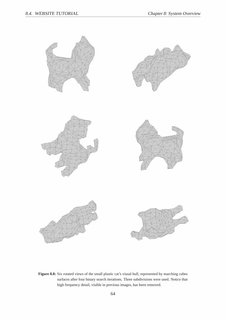
8.4. WEBSITE TUTORIAL Chapter 8: System Overview
Figure 8.8: Six rotated views of the small plastic cat’s visual hull, represented by marching cubes
surfaces after four binary search iterations. Three subdivisions were used. Notice that
high frequency detail, visible in previous images, has been removed.
64

Chapter 8: System Overview 8.4. WEBSITE TUTORIAL
1 Subdivision 2 Subdivisions 3 Subdivisions 4 Subdivisions
Voxels
MC0
MC1
MC2
MC3
Figure 8.9: The 3D marching cubes visual hull models of the imaged cat are shown. Each column
shows the visual hull at an increasing subdivision level ranging from 2 to 5. The first
row shows the voxel-based visual hull models. The rows that follow, show marching
cubes surfaces as more iterations of the binary search are applied. Surface colours
indicate from which category in FigureA.1 the surface is from.
65

8.4. WEBSITE TUTORIAL Chapter 8: System Overview
66

Chapter 9
Experimental Results
This chapter describes the results obtained from the algorithm at three different stages.
RMS and absolute mean percentage error measurements are calculated and compared. The aver-
age time used to compute each volume is also provided. Confidence intervals at 95% are made.
Abbreviations are used for each stage of the algorithm.Voxels is an abbreviation for “Voxel
Based Visual Hull”. MC-0 indicates the standard marching cubes algorithm was used and MC-1,
MC-2 and MC-3 indicate the iterations of the binary search. The binary search is split into three
levels so as to provide a better analysis of its performance.
9.1 Test Data Set
The stages of the algorithm were tested on a data set of 203 stones. The data set was selected so
that it represented a wide distribution of shapes that occur naturally. The average dimensions of
each stone was approximately4mm×4mm×4mm= 64mm3. Each stone was put through a six
camera system six times and the average volume was used as the computed volume ((Vm). All
computations were done offline. Ground truth volumes (Vgt) for the entire batch of stones were
calculated using Archimedes’ Principal:
A body wholly or partially immersed in a fluid will be buoyed up by a force equal to
the weight of the fluid that the body displaces.
Stones were individually weighed in air and then in water. The accuracy of this measuring
system was not tested and these volumes were used as ground truth measurements. Weight
67

9.2. ERROR COMPARISONS Chapter 9: Experimental Results
measurements were taken in10−4× grams, while volumes were measured in cubic millimetres.
Using equation9.1, the volume of each stone was computed.
Vgt = 103×Wair −Wwater
104 (mm3) (9.1)
9.2 Error Comparisons
Percentage error values are tabulated in table9.1and9.2. Volume errors tend to be biased toward
larger stones that produce larger errors, while percentage errors remain unaffected. Percentage
errors were calculate using
%E =V−Vgt
Vgt×100% (9.2)
RMS percentage errors were calculated using
%ERMS=
√√√√√N∑
i=1
(Vi−Vgti
Vgti
)2
N×100% (9.3)
whereN is the sample size. Absolute mean errors were calculated using equation9.4.
%EAVG =
N∑
i=1
∣∣∣Vi−VgtiVgti
∣∣∣N
×100% (9.4)
The visual hull is usually an over estimates of an object’s volume. Due to this characteristic, the
computed visual hull values (Vm) are biased. To compensate for this, the values calculated are
scaled by an average ratio (r) of ground truth values to measured values, to produce an estimated
volume (Vest). It is shown that the estimated volumes are a better approximation to the actual
volumes.
r =Vgt
Vm(9.5a)
Vest = Vm× r (9.5b)
68

Chapter 9: Experimental Results 9.2. ERROR COMPARISONS
Tables9.1and9.2provide RMS and absolute mean error percentages for the measured volumes
(Vm), while tables9.3 and9.4 provide the same errors for the estimated volume(Vest). In each
table, columns represent the stage of the algorithm and rows represent the subdivision levels.
The errors obtained using(Vest) are far better than those obtained using(Vm).
Res Voxels MC-0 MC-1 MC-2 MC-3
1 518.2% 86.3% 79.3% 78.0% 77.3%
2 277.4% 26.8% 25.7% 25.2% 25.1%
3 120.1% 7.7% 7.3% 7.2% 7.2%
4 60.2% 9.4% 9.4% 9.4% 9.4%
5 33.8% 9.9% 9.9% 9.9% 9.9%
Table 9.1: Comparison of the different percentage RMS errors calculated directly from the com-
puted visual hull volumes (Vm).
Res Voxels MC-0 MC-1 MC-2 MC-3
1 463.2% 85.7% 78.8% 77.7% 77.0%
2 268.7% 16.1% 16.3% 16.3% 16.5%
3 116.9% 5.7% 5.4% 5.4% 5.3%
4 58.3% 7.4% 7.3% 7.3% 7.3%
5 32.3% 8.1% 8.1% 8.1% 8.1%
Table 9.2: Comparison of the different percentage absolute mean errors calculated directly from
the computed visual hull volumes (Vm).
Res Voxels MC-0 MC-1 MC-2 MC-3
1 41.3% 74.9% 39.2% 32.6% 30.4%
2 18.7% 27.3% 25.1% 24.4% 24.1%
3 12.7% 7.6% 7.2% 7.1% 7.1%
4 9.5% 7.2% 7.2% 7.2% 7.3%
5 7.8% 6.6% 6.6% 6.6% 6.6%
Table 9.3: Comparison of the different % RMS errors computed using the estimated volumes
(Vest).
As expected, with an increase in resolution, the accuracy improves. Applying marching cubes to
a voxel-based model reduces the volume approximation error associated with voxel model. As
the subdivision levels increase, the improvements become less pronounced (see table9.5).
Voxels at a subdivision level of between 4 and 5 were calculated to be roughly the size of a
single pixel, showing that at subdivision levels larger than 5, the accuracy of the visual hull is
69

9.2. ERROR COMPARISONS Chapter 9: Experimental Results
RMS Percentage Errors
Subdivision Levels1 2 3 4 5
0%
80%
20%
40%
60%
Voxels
MC0
MC1
MC2
MC3
Figure 9.1: Graph of RMS percentage Errors forVest.
Res Voxels MC-0 MC-1 MC-2 MC-3
1 30.1% 47.1% 26.9% 21.9% 20.4%
2 14.5% 15.1% 12.2% 11.6% 11.4%
3 10.0% 5.6% 5.3% 5.3% 5.3%
4 7.6% 5.3% 5.3% 5.3% 5.3%
5 6.3% 5.2% 5.2% 5.2% 5.2%
Table 9.4: Comparison of the different % absolute errors computed using the estimated volumes
(Vest).
Res Voxels MC-0 MC-1 MC-2 MC-3
1 : 2 22.66% 47.58% 14.05% 8.24% 6.31%
2 : 3 5.99% 19.76% 17.96% 17.26% 17.04%
3 : 4 3.24% 0.40% -0.04% -0.15% -0.20%
4 : 5 1.70% 0.58% 0.61% 0.63% 0.64%
Table 9.5: Comparison of the decrease in % RMS errors forVest with an increase in resolution.
not improved. This is noticeable in the tables that follow where, between these two resolutions,
minimal improvements are made.
70

Chapter 9: Experimental Results 9.2. ERROR COMPARISONS
The marching cubes have a pronounced effect on the voxel-based visual hull at all subdivision
levels. Table9.6shows the effects that each section of the algorithm has on the accuracy of the
visual hull output. The binary search on the triangle vertices also has a larger effect on the models
with a lower subdivision level. At the higher levels, improvements are almost negligible. This
is due to surface voxels being roughly the same size as pixels, and the binary search movements
being extremely small. At higher voxel subdivision levels, the binary search has little effect on
the accuracy due to surface patch movements being less than a pixel. At lower subdivision levels,
the surface patches require a higher number of iterations to converge on the optimum.
Res Voxels to MC-0 MC-0 to MC-1 MC-1 to MC-2 MC-2 to MC-3
1 -33.56% 35.72% 6.60% 2.20%
2 -8.64% 2.19% 0.79% 0.26%
3 5.12% 0.40% 0.09% 0.04%
4 2.27% -0.04% -0.02% -0.01%
5 1.16% -0.01% 0.00% 0.00%
Table 9.6: Comparison of the decrease in % RMS errors forVest between the different stages of
visual hull generation.
9.2.1 Confidence Intervals
In order to find a measure of how valid the error percentages are, an interval of values that have
a 95% probability of containing the true mean of RMS percentage errors is computed. Intervals
were calculated using the Student’s t-statistic combined with the method of batch means, which
applies the central limit theorem [15].
The confidence interval assumes a normally distributed population of samples. Since the popula-
tion of squared percentage errors consists of only positive near zero values, the method of batch
means is applied, resulting in a near normal distribution of means. The central limit theorem
implies that the sample mean is approximately Gaussian. The population was split into seven
batches of 29 (7×29= 203). The mean of each batch was computed and these values were used
in equation9.6. Batch means were used to compute the confidence interval as the mean of batch
means in equal to the mean of the total population. Squared percentage errors were obtained
from estimated volume measurements (Vest).
Equation9.6 provides the formula for a(1−α)100% confidence interval. To obtain a95%
confidence interval,α = 0.05. The t-statistic (tα/2) can be found in a lookup table or by using
MATLAB’s TINV function.
71

9.2. ERROR COMPARISONS Chapter 9: Experimental Results
S%E2− tα/2s%E2√
N< µ%E2 < S%E2 + tα/2
s%E2√N
(9.6)
S%E2 is the sample mean of squared percentage errors,s%E2 is the sample standard deviation of
squared percentage errors,µ%E2 is the true population mean of squared percentage errors, andN
is the batch size.
The square root of the above values gives the RMS percentage errors. RMS confidence intervals
at 95% for each method using the estimated volumes (Vest) are shown in tables9.7, 9.8, 9.9, 9.10
and9.11. The size of an interval is indicated in the last column of each table (|Interval|). A plot
for each table is also provided.
Method Resolution of 1 at 95% |Interval|Voxel 36.9%< %ErrorRMS< 45.4% 8.5%
MC-0 63.9%< %ErrorRMS< 84.5% 20.7%
MC-1 35.7%< %ErrorRMS< 42.4% 6.7%
MC-2 30.7%< %ErrorRMS< 34.4% 3.7%
MC-3 26.2%< %ErrorRMS< 34.1% 8.0%
Table 9.7: The 95% confidence intervals ofVest % RMS errors with the resolution at 1 subdivision
level.
RMS Percentage Errors
0%
90%
30%
45%
60%
Voxels MC0 MC1 MC2 MC3
Figure 9.2: Graph of 95% Confidence Intervals for Resolution 1.
72

Chapter 9: Experimental Results 9.2. ERROR COMPARISONS
Method Resolution of 2 at 95% |Interval|Voxel 17.0%< %ErrorRMS< 20.2% 3.2%
MC-0 7.7%< %ErrorRMS< 37.9% 30.2%
MC-1 9.4%< %ErrorRMS< 34.3% 24.9%
MC-2 12.5%< %ErrorRMS< 32.1% 19.6%
MC-3 12.0%< %ErrorRMS< 31.9% 19.8%
Table 9.8: The 95% confidence intervals ofVest % RMS errors with the resolution at 1 subdivision
levels.
RMS Percentage Errors
0%
40%
10%
20%
30%
Voxels MC0 MC1 MC2 MC3
Figure 9.3: Graph of 95% Confidence Intervals for Resolution 2.
Method Resolution of 3 at 95% |Interval|Voxel 11.5%< %ErrorRMS< 13.8% 2.2%
MC-0 6.7%< %ErrorRMS< 8.3% 1.6%
MC-1 6.5%< %ErrorRMS< 7.8% 1.3%
MC-2 6.3%< %ErrorRMS< 7.8% 1.6%
MC-3 6.0%< %ErrorRMS< 8.0% 2.0%
Table 9.9: The 95% confidence intervals ofVest % RMS errors with the resolution at 1 subdivision
levels.
73

9.2. ERROR COMPARISONS Chapter 9: Experimental Results
RMS Percentage Errors
0%
16%
4%
8%
12%
Voxels MC0 MC1 MC2 MC3
Figure 9.4: Graph of 95% Confidence Intervals for Resolution 3.
Method Resolution of 4 at 95% |Interval|Voxel 8.7%< %ErrorRMS< 10.1% 1.4%
MC-0 6.3%< %ErrorRMS< 8.0% 1.7%
MC-1 6.3%< %ErrorRMS< 8.0% 1.7%
MC-2 6.8%< %ErrorRMS< 7.7% 0.9%
MC-3 6.4%< %ErrorRMS< 8.0% 1.6%
Table 9.10:The 95% confidence intervals ofVest % RMS errors with the resolution at 1 subdivision
levels.
Method Resolution of 5 at 95% |Interval|Voxel 6.8%< %ErrorRMS< 8.6% 1.8%
MC-0 5.9%< %ErrorRMS< 7.3% 1.4%
MC-1 6.1%< %ErrorRMS< 7.1% 1.0%
MC-2 6.1%< %ErrorRMS< 7.1% 1.0%
MC-3 6.1%< %ErrorRMS< 7.1% 1.0%
Table 9.11:The 95% confidence intervals ofVest % RMS errors with the resolution at 1 subdivision
levels.
74
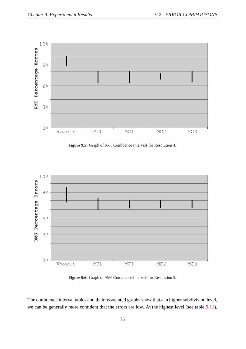
Chapter 9: Experimental Results 9.2. ERROR COMPARISONS
RMS Percentage Errors
0%
12%
3%
6%
9%
Voxels MC0 MC1 MC2 MC3
Figure 9.5: Graph of 95% Confidence Intervals for Resolution 4.
RMS Percentage Errors
0%
10%
3%
5%
8%
Voxels MC0 MC1 MC2 MC3
Figure 9.6: Graph of 95% Confidence Intervals for Resolution 5.
The confidence interval tables and their associated graphs show that at a higher subdivision level,
we can be generally more confident that the errors are low. At the highest level (see table9.11),
75

9.3. TIME COMPARISONS Chapter 9: Experimental Results
the binary search has minimal effect. This is also slightly evident at a subdivision level of 4 (see
table9.10).
9.3 Time Comparisons
Table9.12 contains the average time in seconds required to compute the visual hull for each
method at various subdivision levels.
Res Voxels MC-0 MC-1 MC-2 MC-3
1 0.077s 0.050s 0.052s 0.053s 0.055s
2 0.330s 0.263s 0.277s 0.291s 0.305s
3 1.905s 1.894s 1.956s 2.015s 2.075s
4 14.380s 14.712s 14.966s 15.215s 15.461s
5 114.037s 116.408s 117.458s 118.468s 119.500s
Table 9.12:Speed comparisons for voxels, marching cubes and binary searches. Rows represent
the hull models at increasing subdivision levels. Columns represent the different meth-
ods used.
From this data, tables9.14, 9.15and9.13were generated. Using table9.14, it is clear that the
voxel generation takes up the majority of the time, and by applying marching cubes, the average
difference in time is roughly 10%. The decrease in speed between voxels and marching cubes at
lower subdivision levels is due to the marching cubes algorithm using a smaller output structure.
Table 9.15 shows that the various iterations of the binary search have minimal effect on the
running time of the algorithm.
As expected, table9.13shows that a single increment in subdivision level requires roughly six
times more processing time. This increase in time is shown to be relatively consistent throughout.
9.4 Number of Elements
Table9.16shows how, as the subdivision level increases, the ratio of voxel elements to surface
patches decreases. This means that the marching cubes algorithm uses less elements than voxel-
based methods as the resolution increases.
At lower subdivision levels, a voxel-based model requires fewer voxel elements to build the
visual hull than marching cubes requires surfaces. As the level increases, the ratio decreases.
76

Chapter 9: Experimental Results 9.4. NUMBER OF ELEMENTS
Res Voxels MC-0 MC-1 MC-2 MC-3 Avg
1 : 2 330% 423% 431% 444% 454% 417%
2 : 3 477% 619% 607% 593% 581% 576%
3 : 4 655% 677% 665% 655% 645% 659%
4 : 5 693% 691% 685% 679% 673% 684%
Avg 539% 602% 597% 593% 588% 584%
Table 9.13:This table shows the effect that an increase in subdivision level has on the compu-
tational time. Rows represent the percentage increase in processing time required to
compute the visual hull. Columns represent the different methods used.
Res Voxel to MC
1 -34%
2 -20%
3 -1%
4 2%
5 2%
Avg -10%
Table 9.14:This table shows the percentage increase in time required when applying the marching
cubes algorithm to a voxel-based visual hull model.
Res MC-0 to MC-1 MC-1 to MC-2 MC-2 to MC-3 Avg
1 3% 3% 3% 3%
2 5% 5% 5% 5%
3 3% 3% 3% 3%
4 2% 2% 2% 2%
5 1% 1% 1% 1%
Avg 2.828% 2.649% 2.642% 2.706%
Table 9.15:This table shows the effect that the various iterations of the binary search have on the
time required to compute the visual hull.
This is due to the voxel model having a high number of interior voxels which have no surface
passing through them. In a visual hull model, the relationship between the ratio of voxels to
surface patches is affected by the relationship between the objects surface area and it volume.
An object with a large surface area relative to a low volume will have less triangular patches in
its surface than voxel elements (e.g. a cat). The opposite is true of an object with a small surface
area relative to a large volume (e.g. a sphere).
77

9.4. NUMBER OF ELEMENTS Chapter 9: Experimental Results
Res Voxels MC
1 9 9
2 48 86
3 228 363
4 1348 1509
5 9078 6233
Table 9.16:The average number of elements for voxels vs marching cubes at various subdivision
levels.
78

Chapter 10
Conclusions
A system is presented that allows for the fast computation of an object’s visual hull from multiple
view silhouette images. The algorithm is analysed at three key stages:
• Voxelisation of a volume that contains the target.
• Approximation of the surface passing through exterior voxels.
• Positional accuracy of the surface is improved with a binary search.
As can be seen in the results, a high resolution voxel-based visual hull is computationally very
expensive when compared to the visual hull produced by the marching cubes algorithm at a
similar accuracy percentage. It was also found that the binary search has a negligible effect on
the amount of time required.
The visual hull model, computed with the marching cubes algorithm, using a voxel subdivision
level of 3 and a binary search with 3 iterations, has an RMS error with a 95% chance of being
between 6% and 8%. This visual hull took, on average,1.78% of the time to compute as the
voxel-based model with an equivalent error. Visual hull models with 5 subdivision levels and
binary search iterations of 2 and 3 produce the most accurate results, but require the largest
amount of time to compute.
An advantage of the marching cubes algorithm is that the visual hull it represents is compu-
tationally easier to manipulate than a voxel-based visual hull. The binary search improves the
positional accuracy of each vertex and hence gives a better approximation to the actual surface
that passes through the voxel. Its effects are less noticeable at higher subdivision levels.
79

10.1. LIMITATIONS Chapter 10: Conclusions
10.1 Limitations
Representing an object’s visual hull with a number of voxels is a simple concept, and easily
implemented. The large number of voxels used to make up the visual hull can cause other
systems using these models to become sluggish. When rendering a voxel-based model, only
surface voxels are visible. Internal voxels are useful when computing the centroid or volume of
a model, but are otherwise redundant.
The marching cubes algorithm requires all voxels to be the same size, resulting in the octree
structure losing its advantage of compression. The octree structure provides no consistent notion
of object connectivity, which means that each voxel is tested as a completely separate entity
causing a large number of shared vertices to be repetitively tested. Another limitation of this data
structure is that, if a minimum subdivision level is specified, parts of the object can be omitted and
cause inconsistencies. The marching cubes sections of the algorithm inherit the inconsistencies
and can produce unreliable results. The same problems occur due to assumptions made about a
voxel’s occupancy category. Objects with snake-like extrusions or with sharp peaks can appear
discontinuous at lower resolutions (see Figure5.4).
As in the standard MC15 algorithm, this algorithm’s computational expenses can be reduced by
minimising the number of triangles contained in lookup table surfaces. The use of polygons in
place of triangles is also an option.
10.2 Scope for Further Investigation
Speed improvements for computing a voxel model can be achieved by excluding already com-
puted shared vertices. Including some notion of voxel connectivity makes this feasible.
Texture mapping sections of the imaged object onto the visual hull would improve the visual
effects of the output, making it more pleasing to the eye. This can be done by projecting a
surface patch into the camera image with the best view of the patch. All pixel values inside
the boundary of the patch are then used as texture for the patch. The best camera view can be
determined by projecting the patch normal and finding the minimum angle between the projected
normal and each camera’s optical axis.
80

Appendix A
Chernyaev’s MC33 Marching Cube
Surfaces
81

Chapter A: Chernyaev’s MC33 Marching Cube Surfaces
0 1 2 3.0 3.1
4.0 4.1 5 6.0 6.1
6.2 7.0 7.1 7.2 7.3
7.4 8 9 10.0 10.1
10.2 11 12.0 12.1 12.2
12.3 13.0 13.1 13.2 13.3
13.4 13.5 14
Figure A.1: Chernyaev’s 33 marching cube surfaces[16].
82

Appendix B
Lookup Table for the MC33 Cube
Categories
83

Chapter B: Lookup Table for the MC33 Cube Categories
Case Face Test Interior Test Sub-Case No. of Triangles
1st 2nd 3rd
0 0
1 1
2 2
3 - 3.1 2
+ 3.2 4
4 - 4.1 2
+ 4.2 6
5 3
6 - - 6.1.1 3
- + 6.1.2 7
+ 6.2 5
7 - - - 7.1 3
+ - - 7.2 5
- + - 7.2 5
- - + 7.2 5
+ + - 7.3 9
+ - + 7.3 9
- + + 7.3 9
+ + + + 7.4.1 9
+ + + - 7.4.2 9
8 2
9 4
10 + + 10.1.1 4
- - - 10.1.1 4
- - + 10.1.2 8
+ - 10.2 8
- + 10.2 8
11 4
12 + + 12.1.1 4
- - - 12.1.1 4
- - + 12.1.2 8
+ - 12.2 8
- + 12.2 8
13 45 subcases, testing all the 6 faces and eventually the interior.
14 4
Table B.1: A reduced representation of the test table. Case 13 has 45 entries to map the results of
all the possible tests to the right subcase[23].
84

Bibliography
[1] Narendra Ahuja and Jack Veenstra. Generating octrees from object silhouettes in or-
thographic views. IEEE Transactions on Pattern Analysis and Machine Intelligence,
11(2):137–149, February 1989.
[2] Mark D. Anderson. Delineation of the left ventricle using snakes. The University of Cape
Town, October 2001. Bachelor’s Thesis.
[3] B.G. Baumgart.Geometric Modelling for Computer Vision. PhD thesis, Stanford Univer-
sity, 1974.
[4] Ricardo Chavarriaga and Raquel Urtasun. Camera calibration. Technical report, Graduate
School in Computer Science, Switzerland, January 2001.
[5] Evgeni V. Chernyaev. Marching cubes 33: Construction of topologically correct isosur-
faces. Technical report, 1995. CERN CN 95-17, CERN.
[6] Kong Man Cheung.Visual Hull Construction, Alignment and Refinement for Human Ki-
netic Modelling, Motion Tracking and Rendering.PhD thesis, Carnegie Mellon University,
June 2003.
[7] Oliver Faugeras and Quang-Tuan Luong.The Geometry of Multiple Images. The MIT
Press, 2001.
[8] Keith Forbes, Anthon Voigt, and Ndimi Bodika. An inexpensive, automatic and accurate
camera calibration method. InProceedings of the Thirteenth Annual South African Work-
shop on Pattern Recognition, pages 1–6. PRASA, November 2002. ISBN 0-7992-2147-3.
[9] David A. Forsyth and Jean Ponce.Computer Vision - A Modern Approach. Prentice Hall,
2003.
[10] M.G. Hamblin and G.W. Stachowiak. Variation of particle shape parameters when viewed
as a projection and a section.Journal of Computer-Assisted Microscopy, 6(2):51–59, 1994.
85

BIBLIOGRAPHY BIBLIOGRAPHY
[11] F. Lanaro and P. Tolppanen. 3D characterization of coarse aggregates.Engineering Geology
65, 2001.
[12] John Zaniewskic Larry Bantaa, Ken Chengb. Estimation of limestone particle mass from
2D images. Technical report, Powder Technology, November 2002.
[13] Aldo Laurentini. The visual hull: A new tool for contour-based image understanding. In
7th Scandinavian Conference on Image Analysis, pages 993–1002, 1991.
[14] Aldo Laurentini. The visual hull concept for silhouette-based image understanding. In
IEEE Transactions on Pattern Analysis and Machine Intelligence, volume 16, pages 150–
162, February 1994. Also available at http://www.polito.it/bottino/Articles/pami94.pdf.
[15] Alberto Leon-Garcia. Probability and Random Processes for Electrical Engineering.
Adison-Wesley Publishing Company, 2nd edition, May 1994. ISBN 0-201-50037-X.
[16] Thomas Lewiner, Hlio Lopes, Antnio Wilson Vieira, and Geovan Tavares. Efficient imple-
mentation of marching cubes cases with topological guarantees.Journal of Graphics Tools,
8(2):1–15, 2003.
[17] Sheue ling Lien and James T. Kajiya. A symbolic method for calculating the integral
properties of arbitrary nonconvex polyhedra.IEEE Computer Graphics and Applications,
4(10):35–41, October 1984.
[18] William E. Lorensen and Harvey E. Cline. Computer graphics.Marching Cubes: A High
Resolution 3D Surface Reconstruction, 21(4):163–166, July 1987.
[19] Chien-Ping Lu, Gregory D. Hager, and Eric Mjolsness. Fast and globally convergent pose
estimation from video images.IEEE Transactions on Pattern Analysis and Machine Intel-
ligence, 22(6):610–622, June 2000.
[20] W. N. Martin and J. K. Aggarwal. Volumetric descriptions of objects from multiple views.
In IEEE Transactions on Pattern Analysis and Machine Intelligence, volume 5, pages 150–
158, March 1983.
[21] Wojciech Matusik, Chris Buehler, and Leonard McMillan. Polyhedral visual hulls for real-
time rendering. InProceedings of Twelfth Eurographics Workshop on Rendering, pages
115–125, June 2001.
[22] Phillip Milne. Pixel based segmentation using region growing techniques. The University
of Cape Town, December 2001. Bachelor’s Thesis.
86

BIBLIOGRAPHY BIBLIOGRAPHY
[23] C. Montani, R. Scateni, and R. Scopigno. Discretized marching cubes. In R. D. Berg-
eron and A. E. Kaufman, editors,Visualization ’94 Proceedings, pages 281–287, Wash-
ington D. C., USA, 1994. IEEE Computer Society, IEEE Computer Society Press. cite-
seer.ist.psu.edu/montani94discretized.html.
[24] Gregory. M. Nielson and Bernd. Hamann. The asymptotic decider: Resolving the ambigu-
ity in marching cubes. InProceedings of Visualization ’91, pages 29–38, October 1991.
[25] W. Niem and R. Buschmann. Automatic modelling of 3D natural objects from multiple
views. In European Workshop on Combined Real and Synthetic Image, November 1994.
Hamburg, Germany.
[26] Karin Olsson and Therese Persson. Shape from silhouette scanner. Master’s thesis, Univer-
sity of Linkoping, Sweden, 2001.
[27] Marc Pollefeys.Tutorial on 3D Modelling from Images, June 2000. In conjunction with
ECCV 2000.
[28] Chetana Rao, Erol Tutumluer, and Joseph A. Stefanski. Coarse aggregate shape and size
properties using a new image analyzer.ASTM Journal of Testing and Evaluation, November
2000.
[29] G. Shakhnarovich, L. Lee, and T. Darrell. Integrated face and gait recognition from multiple
views. InIEEE Computer Society Conference on Computer Vision and Pattern Recognition,
2001.
[30] Daniel E. Small. Real time shape from silhouette. Master’s thesis, The University of New
Mexico, July 2001.
[31] M. Tarini, M. Callieri, C. Montani, C. Rocchini, K. Olsson, and T. Persson. Marching
intersections: An efficient approach to shape-from-silhouette. In7th International Fall
Workshop on Vision, Modeling, and Visualization, November 2002.
[32] Emanuele Trucco and Alessandro Verri.Introductory Techniques for 3D Computer Vision.
Prentice Hall PTR, 1998. ISBN 0132611082.
[33] R. Y. Tsai. A versatile camera calibration technique for high-accuracy 3D machine vi-
sion metrology using off-the-shelf TV cameras and lenses.IEEE Journal of Robotics and
Automation, RA-3(4):232–344, August 1987.
[34] Kwan-Yee Kenneth Wong.Structure and Motion from Silhouettes. PhD thesis, University
of Cambridge, 2001.
87

![GPU-accelerated data expansion for the Marching Cubes ... · Extract iso-surface via Marching Cubes Scalar field is sampled over 3D grid Marching Cubes [Lorensen87] —Marches through](https://img.pdfslide.net/doc/110x75/5f59a4a397733378820cfae2/gpu-accelerated-data-expansion-for-the-marching-cubes-extract-iso-surface-via.jpg)