Visualization of shaped data by a rational cubic spline interpolation

Computers & Graphics 25 (2001) 833–845

Technical Section

Visualization of shaped data by a rational cubic splineinterpolation

M. Sarfraza,*, S. Buttb, M.Z. Hussainc

aDepartment of Information and Computer Science, King Fahd University of Petroleum and Minerals, KFUPM # 1510,

Dhahran 31261, Saudi ArabiabUniversity of Engineering, Lahore, PakistancUniversity of the Punjab, Lahore, Pakistan

Abstract

A smooth curve interpolation scheme for positive and monotonic data has been developed. This scheme usespiecewise rational cubic functions. The two families of parameters, in the description of the rational interpolant, havebeen constrained to preserve the shape of the data. The rational spline scheme has a unique representation. In addition

to preserve the shape of positive and/or monotonic data sets, it also possesses extra features to modify the shape of thedesign curve as and when desired. The degree of smoothness attained is C1: r 2001 Elsevier Science Ltd. All rightsreserved.

Keywords: Data visualization; Rational spline; Interpolation; Positive; Monotone

1. Introduction

Smooth curve representation, to visualize the scientific

data, is of great significance in the area of computergraphics and in particular data visualization. Particu-larly, when the data is obtained from some complex

function or from some scientific phenomena, it becomescrucial to incorporate the inherited features of the data.Moreover, smoothness is also one of the very importantrequirements for pleasing visual display. Ordinary spline

schemes, although smoother, are not helpful for theinterpolation of the shaped data. Extremely misguidedresults, violating the inherited features of the data, can

be seen when undesired oscillations occur. For example,for the positive data set in Table 1, the correspondingcurve in Fig. 1 is not as may be desired by the user for a

positive data. The user would be interested to visualize itas it is displayed in Fig. 2. Thus, unwanted oscillationswhich completely destroy the data features, are needed

to be controlled. Another example is the monotonically

increasing data set in Table 2. The correspondingtraditional spline curve is shown in Fig. 3, which hasdestroyed the features of monotonicity as may be

desired corresponding to Fig. 4.This paper examines the problem of shape preserva-

tion of positive as well as monotonic data sets. Various

authors have worked in the area of shape preservation[1–17]. In this paper, the shape preserving interpolationhas been discussed for positive and monotonic data,using rational cubic spline. The motivation to this work

is due to the past work of many authors, e.g. quadraticinterpolation methodology has been adopted in [1,15]for the shape preserving curves. Fritsch and Carlson [3]

and Fritsch and Butland [5] have discussed the piecewisecubic interpolation to monotonic data. Also, Passowand Roulier [2] considered the piecewise polynomial

interpolation to monotonic and convex data. Inparticular, an algorithm for quadratic spline interpola-tion is given in McAllister and Roulier [1]. An

alternative to the use of polynomials, for the interpola-tion of monotonic and convex data, is the application ofpiecewise rational quadratic and cubic functionsby Gregory [4]. Rational functions have been discussed

by Sarfraz [9] in a parametric context.

*Corresponding author. Tel.: +966-3-860-2763; fax: +966-

3-860-2174.

E-mail address: [email protected] (M. Sarfraz).

0097-8493/01/$ - see front matter r 2001 Elsevier Science Ltd. All rights reserved.

PII: S 0 0 9 7 - 8 4 9 3 ( 0 1 ) 0 0 1 2 5 - X

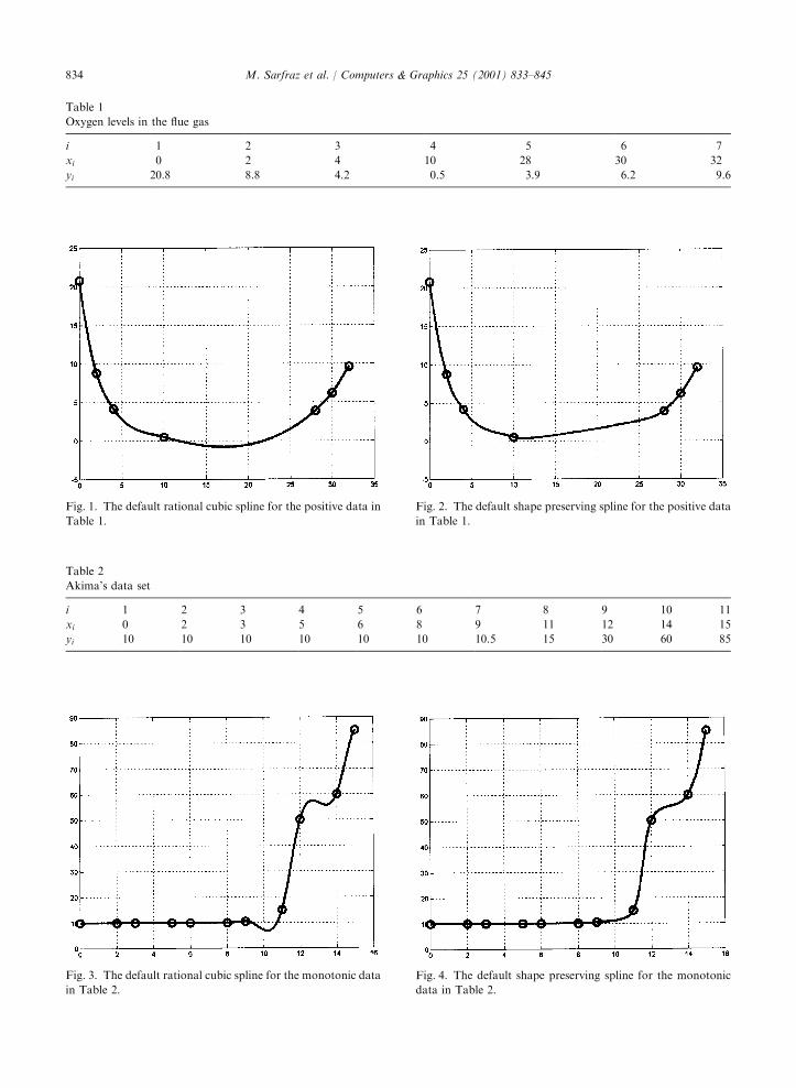
Fig. 1. The default rational cubic spline for the positive data in

Table 1.

Table 1

Oxygen levels in the flue gas

i 1 2 3 4 5 6 7

xi 0 2 4 10 28 30 32

yi 20.8 8.8 4.2 0.5 3.9 6.2 9.6

Fig. 2. The default shape preserving spline for the positive data

in Table 1.

Table 2

Akima’s data set

i 1 2 3 4 5 6 7 8 9 10 11

xi 0 2 3 5 6 8 9 11 12 14 15

yi 10 10 10 10 10 10 10.5 15 30 60 85

Fig. 3. The default rational cubic spline for the monotonic data

in Table 2.

Fig. 4. The default shape preserving spline for the monotonic

data in Table 2.

M. Sarfraz et al. / Computers & Graphics 25 (2001) 833–845834

The theory of methods, in this paper, has number ofadvantageous features. It produces C1 interpolant. No

additional points (knots) are needed. In contrast, thequadratic spline methods of Schumaker [6] and the cubicinterpolation method of Brodlie and Butt [7] require the

introduction of additional knots when used as shapepreserving methods. The interpolant is not concernedwith an arbitrary degree as in [4]. It is a rational cubicwith cubic numerator and cubic denominator. The

rational spline curve representation is bounded andunique in its solution.

The paper begins with a definition of the rational

function in Section 2, where the description of rationalcubic spline, which does not preserve the shape of apositive and/or monotone data, is made. Although this

rational spline was discussed in Sarfraz [16], it was in theparametric context which was useful for the designingapplications. This section reviews it for the scalar

representation so that it can be utilized to preserve thescalar valued data. The positivity problem is discussed inSection 3 for the generation of a C1 spline which canpreserve the shape of a positive data. The sufficient

constraints, on the shape parameters, have been derivedto preserve and control the positive interpolant. Themonotonicity problem is discussed in Section 4 for the

generation of a C1 spline which can preserve the shapeof a monotonic data. The sufficient constraints, in thissection, lead to a monotonic spline solution. The Section

5 discusses and demonstrates the scheme when a data sethas both features of positivity as well as monotonicity.The Section 6 concludes the paper.

2. Rational cubic spline with shape control

Let ðxi; fiÞ; i ¼ 1; 2;y; n; be a given set of data points,

where x1ox2o?oxn: Let

hi ¼ xiþ1 � xi; Di ¼fiþ1 � fi

hi; i ¼ 1; 2;y; n� 1: ð1Þ

Consider the following piecewise rational cubic func-tion:

sðxÞ � siðxÞ

¼Uið1 � yÞ3 þ viViyð1 � yÞ2 þ wiWiy

2ð1 � yÞ þ Ziy3

ð1 � yÞ3 þ viyð1 � yÞ2 þ wiy2ð1 � yÞ þ y3

;

ð2Þ

where

y ¼x� xihi

: ð3Þ

To make the rational function (2) C1; one needs toimpose the following interpolatory properties:

sðxiÞ ¼ fi; sðxiþ1Þ ¼ fiþ1;

sð1ÞðxiÞ ¼ di; sð1Þðxiþ1Þ ¼ diþ1; ð4Þ

which provide the following manipulations:

Ui ¼ fi; Zi ¼ fiþ1;

Vi ¼ fi þhidivi

; Wi ¼ fiþ1 �hidiþ1

wi; ð5Þ

where sð1Þ denotes derivative with respect to x and didenotes derivative value given at the knot xi: This leadsthe piecewise rational cubic (2) to the followingpiecewise Hermite interpolant sAC1½x1; xn�:

sðxÞ � siðxÞ ¼PiðyÞQiðyÞ

; ð6Þ

where

PiðyÞ ¼ fið1 � yÞ3 þ viViyð1 � yÞ2 þ wiWiy2ð1 � yÞ

þ fiþ1y3;

QiðyÞ ¼ ð1 � yÞ3 þ viyð1 � yÞ2 þ wiy2ð1 � yÞ þ y3:

The parameters vi’s, wi’s, and the derivatives di’s are tobe chosen such that the monotonic shape is preserved by

the interpolant (6). One can note that when vi ¼ wi ¼ 3;the rational function obviously becomes the standardcubic Hermite polynomial. Variation for the values of

vi’s and wi’s control (tighten or loosen) the curve indifferent pieces of the curve. This behaviour can be seenin the following subsection:

2.1. Shape control analysis

The parameters vi’s and wi’s can be utilized properlyto modify the shape of the curve according to the desire

of the user. Their effectiveness, for the shape control atknot points, can be seen that if vi;wi�1-N; then thecurve is pulled towards the point ðxi; fiÞ in the

neighbourhood of the knot position xi: This shapebehaviour can be observed by looking at siðxÞ in Eq. (6).This form is similar to that of a Bernstein–Bezier

formulation. One can observe that when vi;wi�1-N;then Vi and Wi�1-fi:

The interval shape control behaviour can be observedby rewriting siðxÞ in Eq. (6) to the following simplified

form:

sðxÞ ¼ fið1 � yÞ þ fiþ1yþ

½ð1 � yÞðdi � DiÞ þ yðDi � diþ1Þ þ yð1 � yÞDiðwi � viÞ�hiyð1 � yÞQiðyÞ

:

ð7Þ

When both vi and wi-N; it is simple to see the

convergence to the following linear interpolant:

sðxÞ ¼ fið1 � yÞ þ fiþ1y: ð8Þ

It should be noted that the shape control analysis is validonly if the bounded derivative values are assumed. A

description of appropriate choices for such derivativevalues is made in the following subsection:

M. Sarfraz et al. / Computers & Graphics 25 (2001) 833–845 835

2.2. Determination of derivatives

In most applications, the derivative parameters fdigare not given and hence must be determined eitherfrom the given data ðxi; fiÞ; i ¼ 1; 2;y; n; or by

some other means. In this article, they are computedfrom the given data in such a way that the C1

smoothness of the interpolant (6) is maintained. Thesemethods are the approximations based on various

mathematical theories. The descriptions of such approx-imations are as follows:

2.2.1. Arithmetic mean methodThis is the three-point difference approximation with

di ¼0 if Di�1 ¼ 0 or Di ¼ 0;

ðhiDi�1 þ hi�1DiÞ=ðhi þ hi�1Þ; otherwise; i ¼ 2; 3;y; n� 1

8<:

ð9Þ

and the end conditions are given as

d1 ¼0 if D1 ¼ 0 or sgnðd *

1 ÞasgnðD1Þ;

d *1 ¼ D1 þ ðD1 � D2Þh1=ðh1 þ h2Þ; otherwise:

(

ð10Þ

dn ¼0 if Dn�1 ¼ 0 or sgnðd *

n ÞasgnðDn�1Þ;

d *n ¼ Dn�1 þ ðDn�1 � Dn�2Þhn�1=ðhn�1 þ hn�2Þ; otherwise:

8<:

ð11Þ

2.2.2. Geometric mean method

These are the non-linear approximations which aredefined as follows:

di ¼0 if Di�1 ¼ 0 or Di ¼ 0;

Dhi=ðhi�1þhi Þi�1 Dhi�1=ðhi�1þhi Þ

i ; otherwise; i ¼ 2; 3;y; n� 1

(

ð12Þ

and the end conditions are given as

d1 ¼0 if D1 ¼ 0 or D3;1 ¼ 0;

D1fD1=D3;1gh1=h2 ; otherwise:

(ð13Þ

dn ¼0 if Dn�1 ¼ 0 or Dn;n�2 ¼ 0;

Dn�1fDn�1=Dn;n�2ghn�1=hn�2 ; otherwise;

(ð14Þ

where

D3;1 ¼ ðf3 � f1Þ=ðx3 � x1Þ;

Dn;n�2 ¼ ðfn � fn�2Þ=ðxn � xn�2Þ: ð15Þ

For given bounded data, the derivative approxi-

mations in Subsections 2.2.1 and 2.2.2 are bounded.Hence, for bounded values of the appropriate shapeparameters

vi;wi; i ¼ 1; 2;y; n� 1; ð16Þ

the interpolant is bounded and unique. Therefore, wecan conclude the above discussion in the following:

Theorem 1. For bounded vi;wi; 8i; and the derivativeapproximations in Subsections 2:2:1 and 2:2:2; the spline

solution of the interpolant ð6Þ exists and is unique.

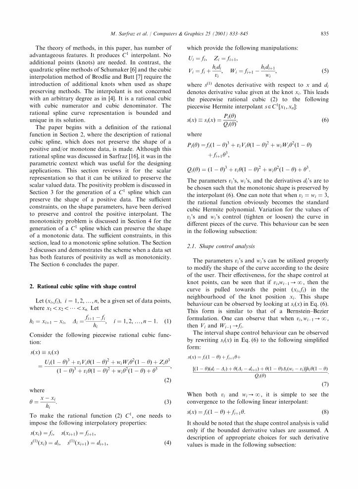
2.3. Examples and discussion

For the demonstration of C1 positive rational cubic

curve scheme, the derivatives will be computed from theSubsections 2.2.1 and 2.2.2, respectively. We will choosethe following choice of shape parameters:

vi ¼ 3 ¼ wi; ð17Þ

to generate the initial default curves. This initial defaultcurve is actually the same as a cubic spline curve.Further modification can be made by changing these

parameters interactively.The Figs. 1 and 3 are the default curves to the positive

and monotonically increasing data in Tables 1 and 2,

respectively. The data in Table 1 has been taken from anexperiment showing oxygen levels in the flue gas (see [7])and the data in Table 2 is another scientific data(Akima’s data) discussed in [3]. It can be seen that the

ordinary spline curves do not guarantee to preserve theshape of the data.

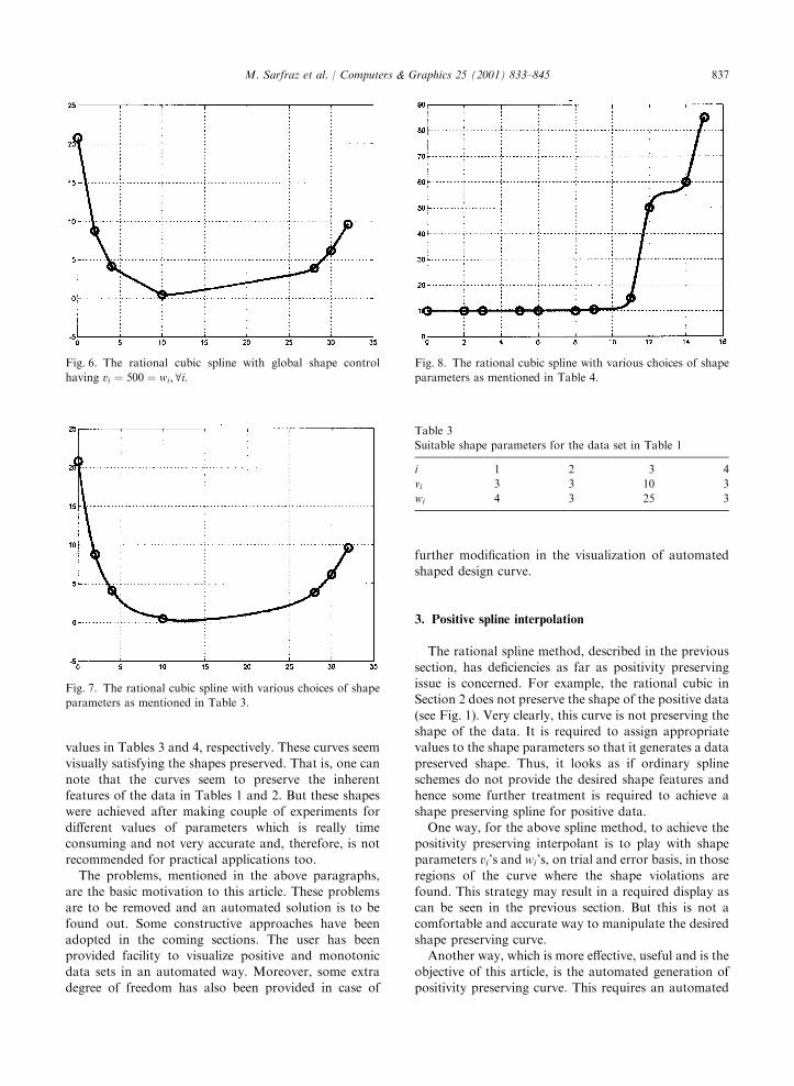
The Figs. 5 and 6 are for the demonstration of global

shape control vi ¼ wi ¼ 25; 500; 8i; respectively. Onecan see that the increasing global values of the shapeparameters gradually pull the curve towards the control

polygon and hence the default curve moves towards thedata preserved curve. But, this way the curve is gettingtightened everywhere which may be undesired.

Another alternate is the allocation of values to theshape parameters according to the nature of the curvebehaviour over various intervals. For example, thecurves in Figs. 7 and 8 are for the shape parameter

Fig. 5. The rational cubic spline with global shape control

having vi ¼ 25 ¼ wi; 8i:


values in Tables 3 and 4, respectively. These curves seemvisually satisfying the shapes preserved. That is, one can

note that the curves seem to preserve the inherentfeatures of the data in Tables 1 and 2. But these shapeswere achieved after making couple of experiments for

different values of parameters which is really timeconsuming and not very accurate and, therefore, is notrecommended for practical applications too.

The problems, mentioned in the above paragraphs,are the basic motivation to this article. These problemsare to be removed and an automated solution is to be

found out. Some constructive approaches have beenadopted in the coming sections. The user has beenprovided facility to visualize positive and monotonicdata sets in an automated way. Moreover, some extra

degree of freedom has also been provided in case of

further modification in the visualization of automatedshaped design curve.

3. Positive spline interpolation

The rational spline method, described in the previous

section, has deficiencies as far as positivity preservingissue is concerned. For example, the rational cubic inSection 2 does not preserve the shape of the positive data

(see Fig. 1). Very clearly, this curve is not preserving theshape of the data. It is required to assign appropriatevalues to the shape parameters so that it generates a data

preserved shape. Thus, it looks as if ordinary splineschemes do not provide the desired shape features andhence some further treatment is required to achieve a

shape preserving spline for positive data.One way, for the above spline method, to achieve the

positivity preserving interpolant is to play with shapeparameters vi’s and wi’s, on trial and error basis, in those

regions of the curve where the shape violations arefound. This strategy may result in a required display ascan be seen in the previous section. But this is not a

comfortable and accurate way to manipulate the desiredshape preserving curve.

Another way, which is more effective, useful and is the

objective of this article, is the automated generation ofpositivity preserving curve. This requires an automated

Fig. 6. The rational cubic spline with global shape control

having vi ¼ 500 ¼ wi ;8i:

Fig. 7. The rational cubic spline with various choices of shape

parameters as mentioned in Table 3.

Fig. 8. The rational cubic spline with various choices of shape

parameters as mentioned in Table 4.

Table 3

Suitable shape parameters for the data set in Table 1

i 1 2 3 4

vi 3 3 10 3

wi 4 3 25 3


computation of suitable shape parameters and derivativevalues. To proceed with this strategy, some mathema-tical treatment is required which will be explained in the

following paragraphs.For simplicity of presentation, let us assume positive

set of data:

ðx1; f1Þ; ðx2; f2Þ;y; ðxn; fnÞ;

so that

x1ox2o?oxn ð18Þ

and

f1 > 0; f2 > 0;y; fn > 0: ð19Þ

In this paper, we shall develop sufficient conditions on

piecewise rational cubics under which C1 positiveinterpolation is preserved. The key idea, to preservepositivity using sðxÞ; is to assign suitable automatedvalues to vi;wi in each interval.

As vi;wi > 0 guarantee strictly positive denominatorQiðyÞ; so initial conditions on vi;wi are

vi > 0; wi > 0 ðvio0;wio0; for positive dataÞ;

i ¼ 1; 2;y; n� 1: ð20Þ

Since QiðyÞ > 0 for all vi;wi > 0; so the positivity of the

interpolant (6) depends on the positivity of cubicpolynomial PiðyÞ: Thus, the problem reduces to thedetermination of appropriate values of vi;wi for which

the polynomial PiðyÞ is positive. Now, PiðyÞ can beexpressed as follows:

PiðtÞ ¼ aiy3 þ biy

2 þ giyþ di; ð21Þ

where

ai ¼ ð1 � wiÞfiþ1 � ð1 � viÞfi þ ðdiþ1 þ diÞhi;

bi ¼ wifiþ1 � ð3 � 2viÞfi � ðdiþ1 þ diÞhi;

gi ¼ dihi � ð3 � viÞfi;

di ¼ fi: ð22Þ

For the strict inequality (for positive data) in (6),

according to Butt and Brodlie [8], PiðyÞ > 0 if and only if

ðP0ið0Þ;P

0ið1ÞÞAR1UR2; ð23Þ

where

R1 ¼ ða; bÞ: a >�3fihi

; bo3fiþ1

hi

� �; ð24Þ

R2 ¼fða; bÞ: 36fifiþ1ða2 þ b2 þ ab� 3Diðaþ bÞ þ 3D2i Þ

þ 3ðfiþ1a� fibÞð2hiab� 3fiþ1aþ 3fibÞ

þ 4hiðfiþ1a3 � fib

3Þ � h2i a

2b2 > 0g: ð25Þ

We have

P0ið0Þ ¼

fihiðvi � 3Þ þ di;

P0ið1Þ ¼ diþ1 �

fiþ1

hiðwi � 3Þ:

Now (23) is true when

ðP0ið0Þ;P

0ið1ÞÞAR1;

P0ið0Þ >

�3fihi

; P0ið1Þo

3fiþ1

hi:

This leads to the following constraints:

vi > mi; wi > Mi; ð26Þ

where

mi ¼ max 0;�hidifi

� �; Mi ¼ max 0;

hidiþ1

fiþ1

� �: ð27Þ

Further

ðP0ið0Þ;P

0ið1ÞÞAR2

if

36fifiþ1½f21ðri; uiÞ þ f2

2ðwiÞ þ f1ðviÞf2ðwiÞ

� 3Diðf1ðviÞ þ f2ðwiÞÞ þ 3D2i �

þ 3½fiþ1f1ðviÞ � yif2ðwiÞ�½2hif1ðviÞf2ðwiÞ

� 3fiþ1f1ðviÞ þ 3fif2ðwiÞ�

þ 4hi½fiþ1f31ðviÞ � yif

32ðwiÞ� � h2

i f21ðviÞf

22ðwiÞ > 0; ð28Þ

where

f1ðviÞ ¼ P0ið0Þ;

f2ðwiÞ ¼ P0ið1Þ: ð29Þ

This leads to the following:

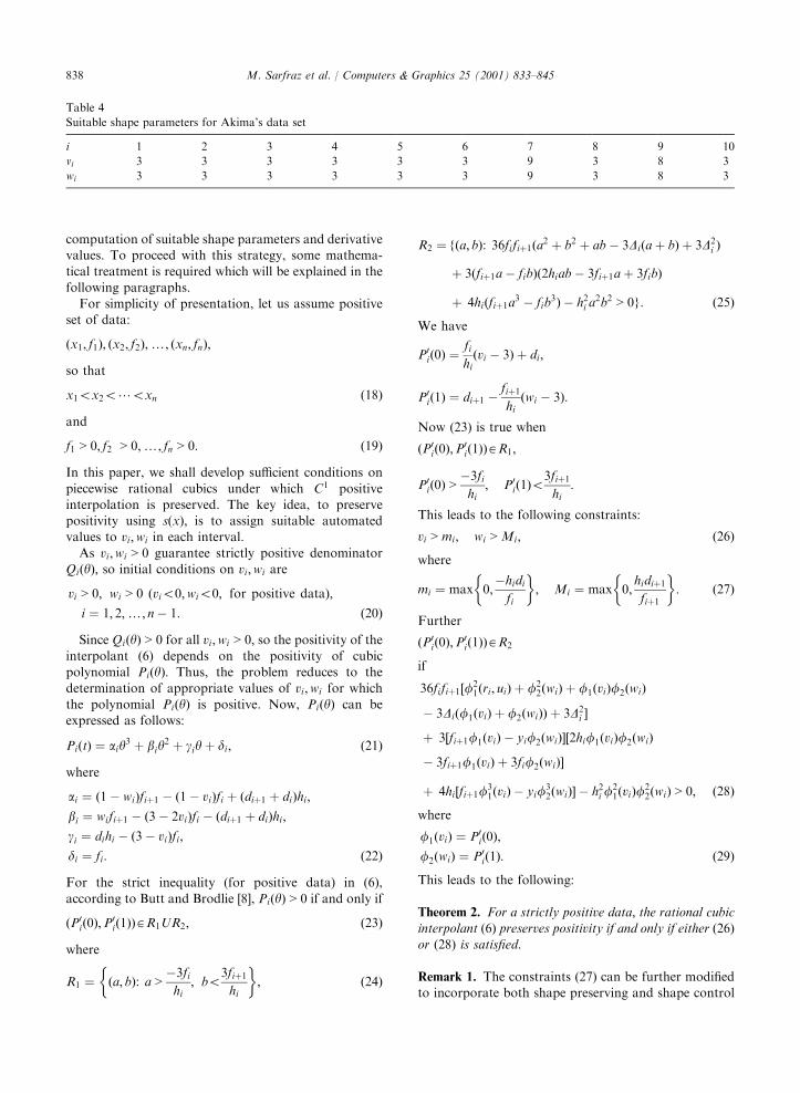
Theorem 2. For a strictly positive data; the rational cubicinterpolant ð6Þ preserves positivity if and only if either ð26Þor ð28Þ is satisfied.

Remark 1. The constraints (27) can be further modifiedto incorporate both shape preserving and shape control

Table 4

Suitable shape parameters for Akima’s data set

i 1 2 3 4 5 6 7 8 9 10

vi 3 3 3 3 3 3 9 3 8 3

wi 3 3 3 3 3 3 9 3 8 3


features. Without loss of generality, one can findparameters ri and qi satisfying

ri; qiX1; ð30Þ

such that the constraints (26) and (27) lead to thefollowing sufficient conditions for the freedom over thechoice of ri and qi:

vi ¼ ð1 þmiÞri; wi ¼ ð1 þMiÞqi: ð31Þ

One can make the choice of ri and qi to be the greatest

lower bound as follows:

ri ¼ 1; qi ¼ 1: ð32Þ

This choice satisfies (26) and it also provides visuallyvery pleasant results. Some more practical sufficientconditions, which satisfy (26) too, are the followings:

vi ¼ wi ¼ 1 þ maxðmiri;MiqiÞ: ð33Þ

Although, these conditions appear to be stronger than(31) but their use has shown quite pleasing results. Formore practical and better results, however, we will utilize

the constraints in (31) as can be seen in the demonstra-tion Subsection 3.1.

Remark 2. Although vi and wi satisfying (28) can be

determined but it requires a lot of computations. Thealternate choice, in Remark 1, provides efficient andreasonably attractive results as can be seen in the

following subsection:

Remark 3. This curve plotting method can be used in

both cases when either di’s are particularly specified orestimated by some method.


We will assume the derivative approximations asmentioned in Subsection 2.2.1. These approximationsare computationally more economical. However, onecan use the derivative choice in Subsection 2.2.1 too.

The scheme has been implemented on the data set ofTable 1. The Fig. 1 is the default rational cubic splinecurve for the choice of parameters in (17), whereas the

Fig. 2 is its corresponding shape preserving splinecurve for the automatic choice of parameters in (31)and (32). The corresponding automatic outputs of

the derivative and shape parameters, for the shapepreserving curves in Fig. 2 is given in Table 5. Thepleasing visualization of the data set (see Fig. 2) is

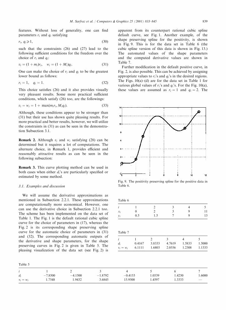
apparent from its counterpart rational cubic splinedefault curve, see Fig. 1. Another example, of the

shape preserving spline for the positivity, is shownin Fig. 9. This is for the data set in Table 6 (thecubic spline version of this data is shown in Fig. 13.)

The automated values of the shape parametersand the computed derivative values are shown inTable 7.

Further modification in the default positive curve, in

Fig. 2, is also possible. This can be achieved by assigningappropriate values to ri’s and qi’s in the desired regions.The Figs. 10(a)–(d) are for the data set in Table 1 for

various global values of ri’s and qi’s. For the Fig. 10(a),these values are assumed as ri ¼ 1 and qi ¼ 2: The

Table 5

i 1 2 3 4 5 6 7

di �7:8500 �4:1500 �1:8792 �0:4153 1.0539 1.4250 1.6000

vi ¼ wi 1.7548 1.9432 3.6845 15.9500 1.4597 1.3333 F

Fig. 9. The positivity preserving spline for the positive data in

Table 6.

Table 6

i 1 2 3 4 5

xi 0 2 3 9 11

yi 0.5 1.5 7 9 13

Table 7

i 1 2 3 4 5

di 0.4167 3.8333 4.7619 1.5833 1.5000

vi ¼ wi 6.1111 1.6803 2.0556 1.2308 1.1333


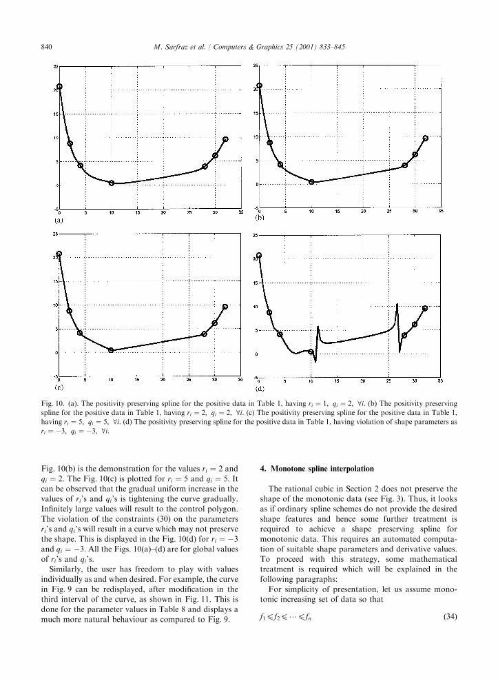
Fig. 10(b) is the demonstration for the values ri ¼ 2 and

qi ¼ 2: The Fig. 10(c) is plotted for ri ¼ 5 and qi ¼ 5: Itcan be observed that the gradual uniform increase in thevalues of ri’s and qi’s is tightening the curve gradually.Infinitely large values will result to the control polygon.

The violation of the constraints (30) on the parametersri’s and qi’s will result in a curve which may not preservethe shape. This is displayed in the Fig. 10(d) for ri ¼ �3

and qi ¼ �3: All the Figs. 10(a)–(d) are for global valuesof ri’s and qi’s.

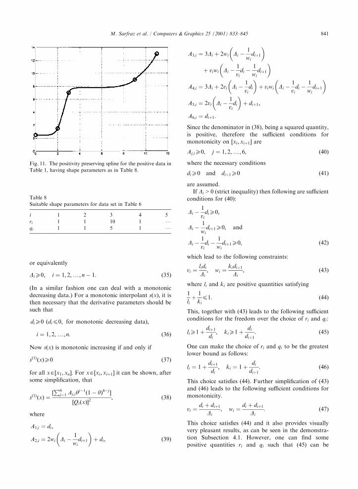
Similarly, the user has freedom to play with values

individually as and when desired. For example, the curvein Fig. 9 can be redisplayed, after modification in thethird interval of the curve, as shown in Fig. 11. This isdone for the parameter values in Table 8 and displays a

much more natural behaviour as compared to Fig. 9.

4. Monotone spline interpolation

The rational cubic in Section 2 does not preserve theshape of the monotonic data (see Fig. 3). Thus, it looksas if ordinary spline schemes do not provide the desired

shape features and hence some further treatment isrequired to achieve a shape preserving spline formonotonic data. This requires an automated computa-

tion of suitable shape parameters and derivative values.To proceed with this strategy, some mathematicaltreatment is required which will be explained in the

following paragraphs:For simplicity of presentation, let us assume mono-

tonic increasing set of data so that

f1pf2p?pfn ð34Þ

Fig. 10. (a). The positivity preserving spline for the positive data in Table 1, having ri ¼ 1; qi ¼ 2; 8i: (b) The positivity preserving

spline for the positive data in Table 1, having ri ¼ 2; qi ¼ 2; 8i: (c) The positivity preserving spline for the positive data in Table 1,

having ri ¼ 5; qi ¼ 5; 8i: (d) The positivity preserving spline for the positive data in Table 1, having violation of shape parameters as

ri ¼ �3; qi ¼ �3; 8i:


or equivalently

DiX0; i ¼ 1; 2;y; n� 1: ð35Þ

(In a similar fashion one can deal with a monotonicdecreasing data.) For a monotonic interpolant sðxÞ; it isthen necessary that the derivative parameters should be

such that

diX0 ðdip0; for monotonic decreasing dataÞ;

i ¼ 1; 2;y; n: ð36Þ

Now sðxÞ is monotonic increasing if and only if

sð1ÞðxÞX0 ð37Þ

for all xA½x1; xn�: For xA½xi;xiþ1� it can be shown, after

some simplification, that

sð1ÞðxÞ ¼½P6

j¼1 Aj;iyj�1ð1 � yÞ6�j �

½QiðxÞ�2; ð38Þ

where

A1;i ¼ di;

A2;i ¼ 2wi Di �1

widiþ1

� þ di; ð39Þ

A3;i ¼ 3Di þ 2wi Di �1

widiþ1

�

þ viwi Di �1

vidi �

1

widiþ1

�

A4;i ¼ 3Di þ 2vi Di �1

vidi

� þ viwi Di �

1

vidi �

1

widiþ1

�

A5;i ¼ 2vi Di �1

vidi

� þ diþ1;

A6;i ¼ diþ1:

Since the denominator in (38), being a squared quantity,

is positive, therefore the sufficient conditions formonotonicity on ½xi; xiþ1� are

Aj;iX0; j ¼ 1; 2;y; 6; ð40Þ

where the necessary conditions

diX0 and diþ1X0 ð41Þ

are assumed.If Di > 0 (strict inequality) then following are sufficient

conditions for (40):

Di �1

vidiX0;

Di �1

widiþ1X0; and

Di �1

vidi �

1

widiþ1X0; ð42Þ

which lead to the following constraints:

vi ¼lidiDi

; wi ¼kidiþ1

Di; ð43Þ

where li and ki are positive quantities satisfying

1

liþ

1

kip1: ð44Þ

This, together with (43) leads to the following sufficientconditions for the freedom over the choice of ri and qi:

liX1 þdiþ1

di; kiX1 þ

didiþ1

: ð45Þ

One can make the choice of ri and qi to be the greatestlower bound as follows:

li ¼ 1 þdiþ1

di; ki ¼ 1 þ

didiþ1

: ð46Þ

This choice satisfies (44). Further simplification of (43)and (46) leads to the following sufficient conditions for

monotonicity.

vi ¼di þ diþ1

Di; wi ¼

di þ diþ1

Di: ð47Þ

This choice satisfies (44) and it also provides visuallyvery pleasant results, as can be seen in the demonstra-

tion Subsection 4.1. However, one can find somepositive quantities ri and qi such that (45) can be

Fig. 11. The positivity preserving spline for the positive data in

Table 1, having shape parameters as in Table 8.

Table 8

Suitable shape parameters for data set in Table 6

i 1 2 3 4 5

ri 1 1 10 1 Fqi 1 1 5 1 F


rewritten as

li ¼ 1 þdiþ1

di

� ri; ki ¼ 1 þ

didiþ1

� qi; ð48Þ

where

ri; qiX1: ð49Þ

Substitution of parameters in (47) into (43) yields thesufficient condition to the followings:

vi ¼di þ diþ1

Di

� ri; wi ¼

di þ diþ1

Di

� qi: ð50Þ

The parameters ri and qi will help out the user in a

further modification of the automated monotone curve.It should be noted that if Di ¼ 0; then it is necessary to

set di ¼ diþ1 ¼ 0; and thus

sðxÞ ¼ fi ¼ fiþ1 ð51Þ

is a constant on ½xi; xiþ1�: Hence the interpolant (6) ismonotonic increasing together with the conditions (41)and (47). For the case where the data is monotonic but

not strictly monotonic (i.e., when some Di ¼ 0) it wouldbe necessary to divide the data into strictly monotonicparts. If we set di ¼ diþ1 ¼ 0 whenever Di ¼ 0; then the

resulting interpolant will be C0 at break points. Theabove discussion can be summarized as:

Theorem 3. Given the conditions ð36Þ on the derivative

parameters; ð47Þ as well as ð50Þ are the sufficientconditions for the interpolant ð6Þ to be monotonicincreasing.


Similarly as in Section 3, we will assume the derivativeapproximations as mentioned in Subsection 2.2.1. The

scheme has been implemented on the data set of Table 2.The Fig. 3 is the default rational cubic spline curve forthe choice of parameters in (17), whereas the Fig. 4 is its

corresponding shape preserving spline curve for theautomatic choice of parameters in (47). The correspond-ing automatic outputs of the derivative and shape

parameters, for the shape preserving curves in Fig. 4 isgiven in Table 9. The pleasing visualization of the dataset (see Fig. 4) is apparent from its counterpart rational

cubic spline default curve, see Fig. 3.Further modification in the default monotone curve,

in Fig. 4, is also possible. This can be achieved byassigning appropriate values to ri’s and qi’s in the

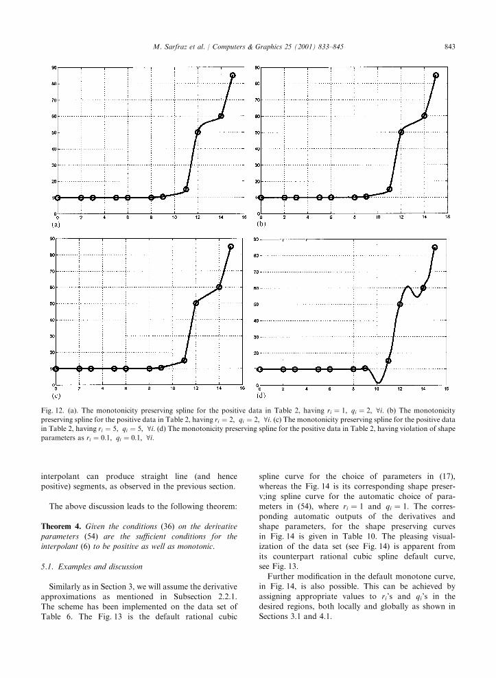
desired regions. The Figs. 12(a)–(d) are for the data set

in Table 2 for various global values of ri’s and qi’s. Forthe Fig. 12(a), these values are assumed as ri ¼ 1 and

qi ¼ 2: The Fig. 12(b) is the demonstration for the valuesri ¼ 2 and qi ¼ 2: The Fig. 12(c) is plotted for ri ¼ 5 andqi ¼ 5: It can be observed that the gradual uniform

increase in the values of ri’s and qi’s is tightening thecurve gradually. Infinitely large values will result to thecontrol polygon. The violation of the constraints (30) onthe parameters ri’s and qi’s will result in a curve which

may not preserve the shape. This is displayed in theFig. 12(d) for ri ¼ 0:1 and qi ¼ 0:1: All the Figs. 12(a)–(d) are for global values of ri’s and qi’s. Similarly, the

user has freedom to play with values individually as andwhen desired.

5. Positive and monotone spline

There may arise certain data which possess the dualfeatures of being positive as well as monotonic at thesame time. Such a set of data ðxi; fiÞ; i ¼ 1; 2;y; n; takesthe following form:

0of1pf2p?pfn; ð52Þ

where

x1ox2o?oxn:

The derivative parameters must then satisfy the follow-ings:

diX0; i ¼ 1; 2;y; n: ð53Þ

One can note (50) that the choice of parameters

vi ¼ 1 þdi þ diþ1

Di

� ri; wi ¼ 1 þ

di þ diþ1

Di

� qi ð54Þ

is also valid to preserve the monotonicity. Moreover,any monotonic interpolant must then also be positive.Thus, the monotonic interpolant of the previous section

is also suitable for the interpolation of positive andmonotonic data. This result is confirmed by comparing(31) and (54) and from the fact that

di þ diþ1

DiXmaxðmi;MiÞ ð55Þ

for the data satisfying (52). Thus, the monotonicityconditions (54) are sufficient to ensure that the positivity

conditions (31) are satisfied.

Remark 4. It should be noted that if the data is

monotonic but not strictly monotonic, then the

Table 9

i 1 2 3 4 5 6 7 8 9 10 11

di 0 0 0 0 0 0 1.0833 24.0833 25.0000 18.3333 12.5000

vi ¼ wi F F F F F 2.1667 11.1852 1.4024 8.6667 0.2333 F


interpolant can produce straight line (and hencepositive) segments, as observed in the previous section.

The above discussion leads to the following theorem:

Theorem 4. Given the conditions ð36Þ on the derivativeparameters ð54Þ are the sufficient conditions for theinterpolant ð6Þ to be positive as well as monotonic.


Similarly as in Section 3, we will assume the derivativeapproximations as mentioned in Subsection 2.2.1.

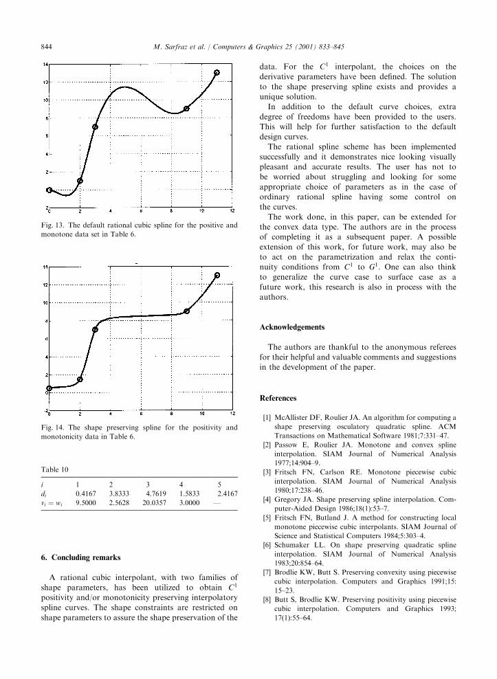
The scheme has been implemented on the data set ofTable 6. The Fig. 13 is the default rational cubic

spline curve for the choice of parameters in (17),whereas the Fig. 14 is its corresponding shape preser-

v;ing spline curve for the automatic choice of para-meters in (54), where ri ¼ 1 and qi ¼ 1: The corres-ponding automatic outputs of the derivatives and

shape parameters, for the shape preserving curvesin Fig. 14 is given in Table 10. The pleasing visual-ization of the data set (see Fig. 14) is apparent from

its counterpart rational cubic spline default curve,see Fig. 13.

Further modification in the default monotone curve,in Fig. 14, is also possible. This can be achieved by

assigning appropriate values to ri’s and qi’s in thedesired regions, both locally and globally as shown inSections 3.1 and 4.1.

Fig. 12. (a). The monotonicity preserving spline for the positive data in Table 2, having ri ¼ 1; qi ¼ 2; 8i: (b) The monotonicity

preserving spline for the positive data in Table 2, having ri ¼ 2; qi ¼ 2; 8i: (c) The monotonicity preserving spline for the positive data

in Table 2, having ri ¼ 5; qi ¼ 5; 8i: (d) The monotonicity preserving spline for the positive data in Table 2, having violation of shape

parameters as ri ¼ 0:1; qi ¼ 0:1; 8i:


6. Concluding remarks

A rational cubic interpolant, with two families ofshape parameters, has been utilized to obtain C1

positivity and/or monotonicity preserving interpolatoryspline curves. The shape constraints are restricted on

shape parameters to assure the shape preservation of the

data. For the C1 interpolant, the choices on thederivative parameters have been defined. The solution

to the shape preserving spline exists and provides aunique solution.

In addition to the default curve choices, extra

degree of freedoms have been provided to the users.This will help for further satisfaction to the defaultdesign curves.

The rational spline scheme has been implemented

successfully and it demonstrates nice looking visuallypleasant and accurate results. The user has not tobe worried about struggling and looking for some

appropriate choice of parameters as in the case ofordinary rational spline having some control onthe curves.

The work done, in this paper, can be extended forthe convex data type. The authors are in the processof completing it as a subsequent paper. A possible

extension of this work, for future work, may also beto act on the parametrization and relax the conti-nuity conditions from C1 to G1: One can also thinkto generalize the curve case to surface case as a

future work, this research is also in process with theauthors.

Acknowledgements

The authors are thankful to the anonymous refereesfor their helpful and valuable comments and suggestionsin the development of the paper.

References

[1] McAllister DF, Roulier JA. An algorithm for computing a

shape preserving osculatory quadratic spline. ACM

Transactions on Mathematical Software 1981;7:331–47.

[2] Passow E, Roulier JA. Monotone and convex spline

interpolation. SIAM Journal of Numerical Analysis

1977;14:904–9.

[3] Fritsch FN, Carlson RE. Monotone piecewise cubic


1980;17:238–46.

[4] Gregory JA. Shape preserving spline interpolation. Com-

puter-Aided Design 1986;18(1):53–7.

[5] Fritsch FN, Butland J. A method for constructing local

monotone piecewise cubic interpolants. SIAM Journal of

Science and Statistical Computers 1984;5:303–4.

[6] Schumaker LL. On shape preserving quadratic spline


1983;20:854–64.

[7] Brodlie KW, Butt S. Preserving convexity using piecewise

cubic interpolation. Computers and Graphics 1991;15:

15–23.

[8] Butt S, Brodlie KW. Preserving positivity using piecewise

cubic interpolation. Computers and Graphics 1993;

17(1):55–64.

Fig. 13. The default rational cubic spline for the positive and

monotone data set in Table 6.

Fig. 14. The shape preserving spline for the positivity and

monotonicity data in Table 6.

Table 10

i 1 2 3 4 5

di 0.4167 3.8333 4.7619 1.5833 2.4167

vi ¼ wi 9.5000 2.5628 20.0357 3.0000 F


[9] Sarfraz M. Convexity preserving piecewise rational inter-

polation for planar curves. Bulletin of Korean Mathema-

tical Society 1992;29(2):193–200.

[10] Sarfraz M. Preserving monotone shape of the data using

piecewise rational cubic functions. Computers and Gra-

phics 1997;21(1):5–14.

[11] Brodlie KW. Methods for drawing curves. In: Earnshaw

RA, editor. Fundamenal algorithm for computer graphics.

Berlin/Heidelberg: Springer, 1985. p. 303–23.

[12] DeVore A, Yan Z. Error analysis for piecewise quadratic

curve fitting algorithms. Computer Aided Geom Design

1986;3:205–15.

[13] Greiner K. A survey on univariate data interpolation and

approximation by splines of given shape. Mathematical

Computation Modelling 1991;15:97–l06.

[14] Constantini P. Boundary-valued shape preserving inter-

polating splines. ACM Transactions on Mathematical

Software 1997;23(2):229–51.

[15] Lahtinen A. Monotone interpolation with application to

estimation of taper curves. Annals of Numerical Mathe-

matics 1996;3:151–61.

[16] Sarfraz M. Interpolatory rational cubic spline with biased,

point and interval tension. Computers and Graphics

1992;16(4):427–30.

[17] Moreton HP, Sequin CH. In: Nick Sapidis, editor.

Minimum variation curves and surfaces for computer-

aided geometric design, Designing Fair Curves and

Surfaces. Proceedings of SIAM’94 Conference. 1995.

p. 123–59.


Documents

Visualization of shaped data by a rational cubic spline interpolation