Volume Illumination & Vector Field Visualisation

Taku Komura Volume Illumination & Vector Vis. 1

Visualisation : Lecture 11

Visualisation – Lecture 11

Taku Komura

Institute for Perception, Action & BehaviourSchool of Informatics

Volume Illumination &Vector Field Visualisation



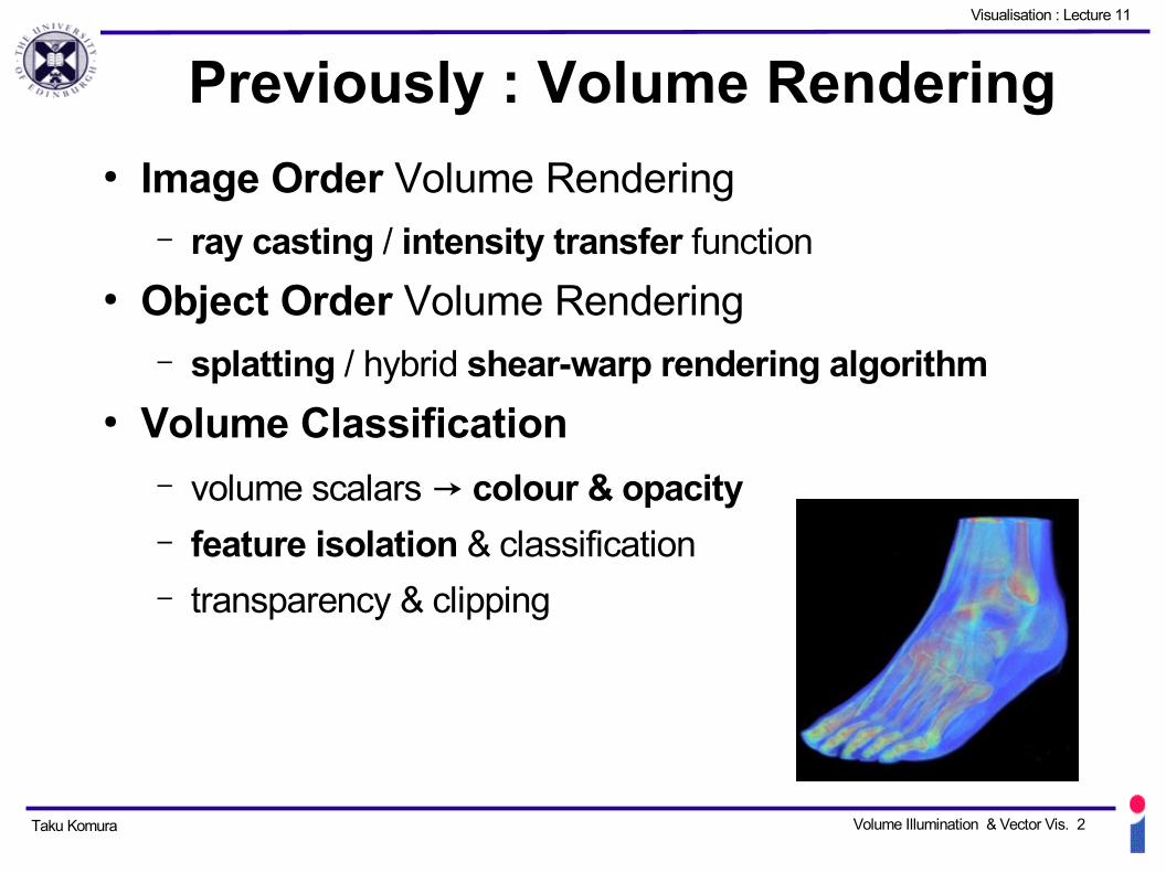
Previously : Volume Rendering● Image Order Volume Rendering

– ray casting / intensity transfer function● Object Order Volume Rendering

– splatting / hybrid shear-warp rendering algorithm● Volume Classification

– volume scalars → colour & opacity– feature isolation & classification– transparency & clipping



Light Propagation in Volumes● Lighting in volume

– only transmission and emission considered (until now)– can also:

— reflect light— scatter light into different directions



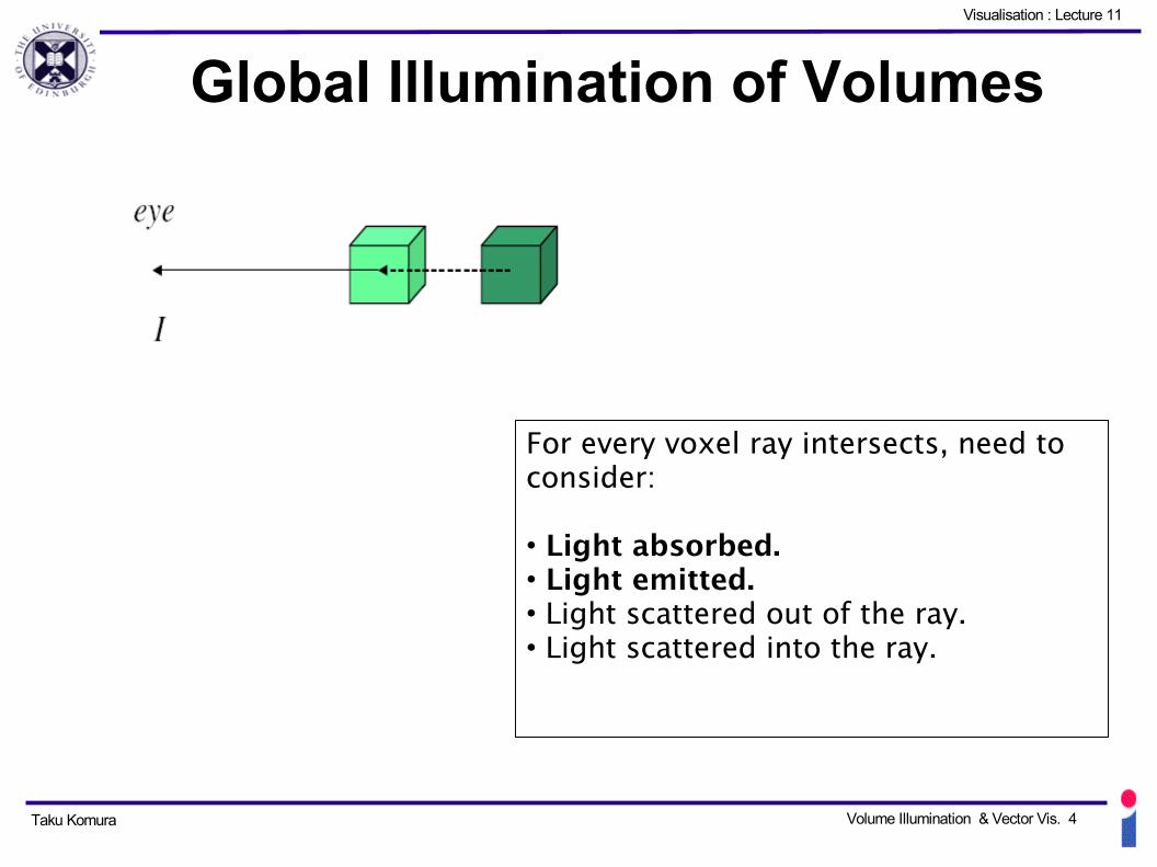
Global Illumination of Volumes

For every voxel ray intersects, need to consider:

• Light absorbed.• Light emitted.• Light scattered out of the ray.• Light scattered into the ray.



Global Illumination of Volumes

For every voxel ray intersects, need to consider:

• Light absorbed.• Light emitted.• Light scattered out of the ray.• Light scattered into the ray.

Normally ignore scattering in volumetric illumination !

Why ? : computational cost



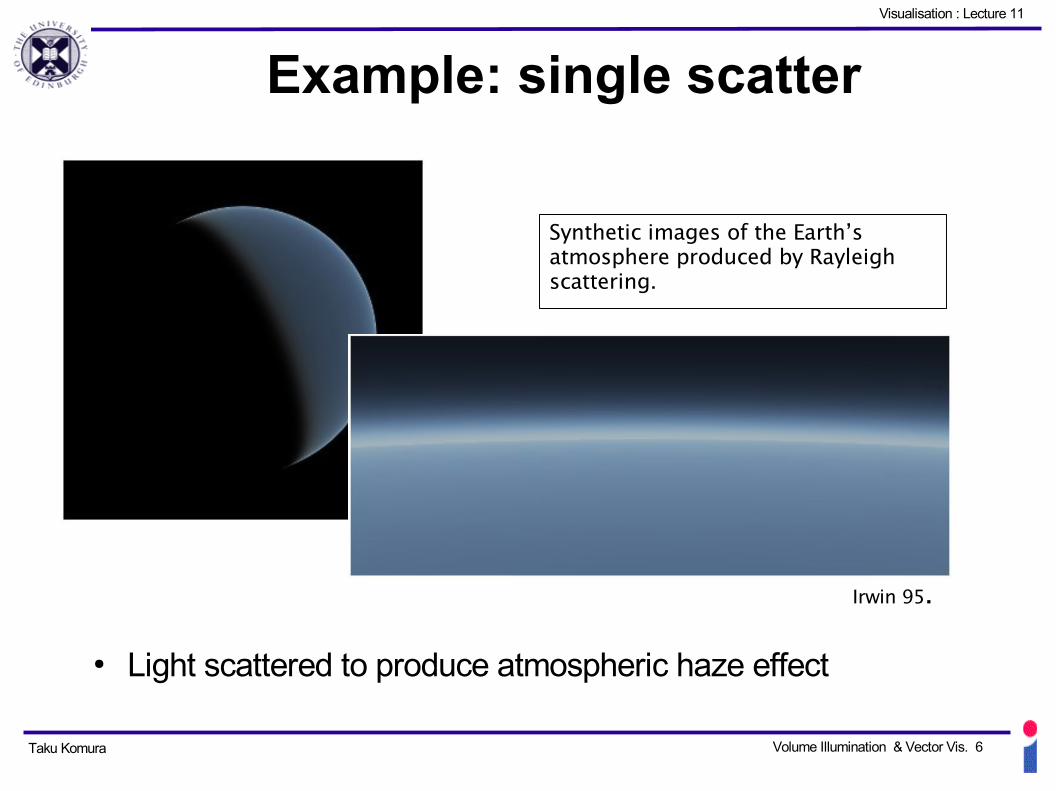
Example: single scatter

● Light scattered to produce atmospheric haze effect

Irwin 95.

Synthetic images of the Earth’s atmosphere produced by Rayleigh scattering.



Example : multiple scattering

● Light scattered multiple times to produce simulation of a cloud

Scattering has scale dependence – can see this is quite a small cloud.



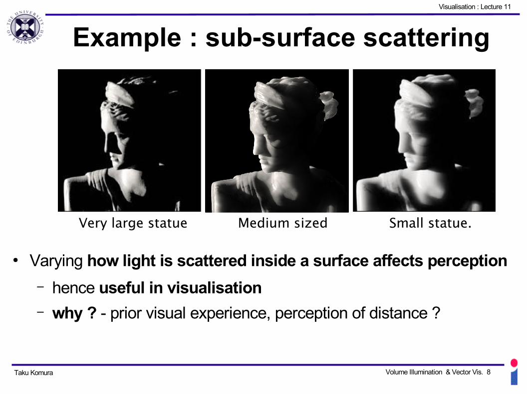
Example : sub-surface scattering

● Varying how light is scattered inside a surface affects perception

– hence useful in visualisation– why ? - prior visual experience, perception of distance ?

Very large statue Medium sized Small statue.



Volume Illumination - ?

● Anyway, scattering is to costly so we usually do not take them into account when doing volume rendering

● But we still can add slight shadows to the volume by illuminating them



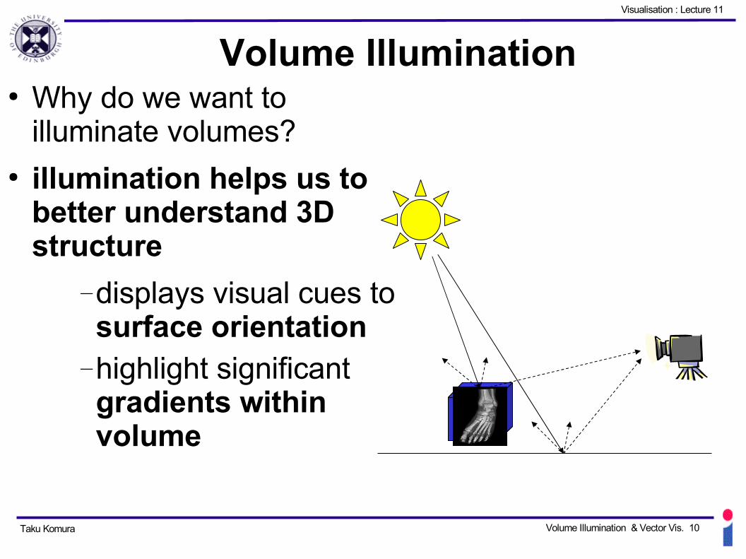
Volume Illumination● Why do we want to

illuminate volumes?● illumination helps us to

better understand 3D structure

—displays visual cues to surface orientation

—highlight significant gradients within volume



What are we illuminating ?

● embedded (iso-) surface● sharp gradients in opacity



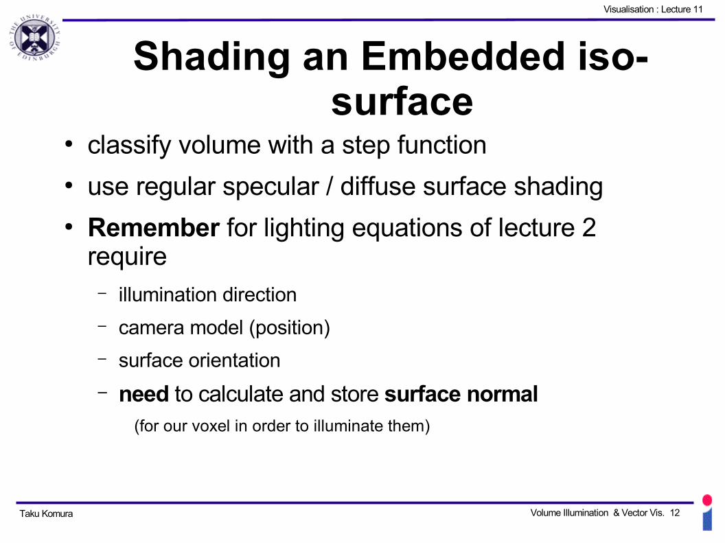
Shading an Embedded iso-surface

● classify volume with a step function● use regular specular / diffuse surface shading● Remember for lighting equations of lecture 2

require– illumination direction

– camera model (position)

– surface orientation

– need to calculate and store surface normal(for our voxel in order to illuminate them)



Estimating the surface normal from distance map

● Use distance map to the iso-surface value

1. Determine the threshold value

2. Determine the surface voxels based on the threshold

3. Compute the normal vectors based on centred difference method

For example, if we sample the centre of the voxels,

z x=12 z x1, y −z x−1, y

z y=12 z x , y1− z x , y−1

N=− zx

zx2 z y

21,

− z y z x

2 z y

21,

1 z x

2 z y

21



Result : illuminated iso-surface

● Surface normals recovered from depth map of surface

– regions of similar curvature taken into consideration

MIP technique

Shaded embedded iso-surface.



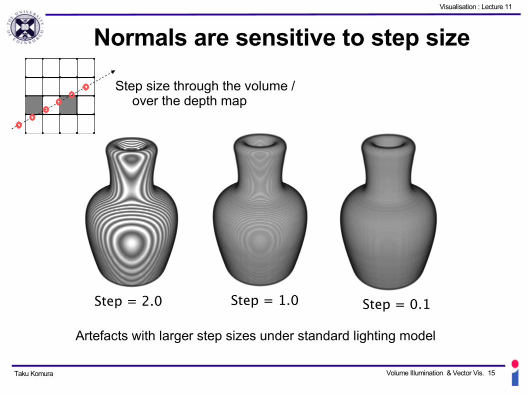
Normals are sensitive to step size

Artefacts with larger step sizes under standard lighting model

Step = 2.0 Step = 1.0 Step = 0.1

Step size through the volume / over the depth map



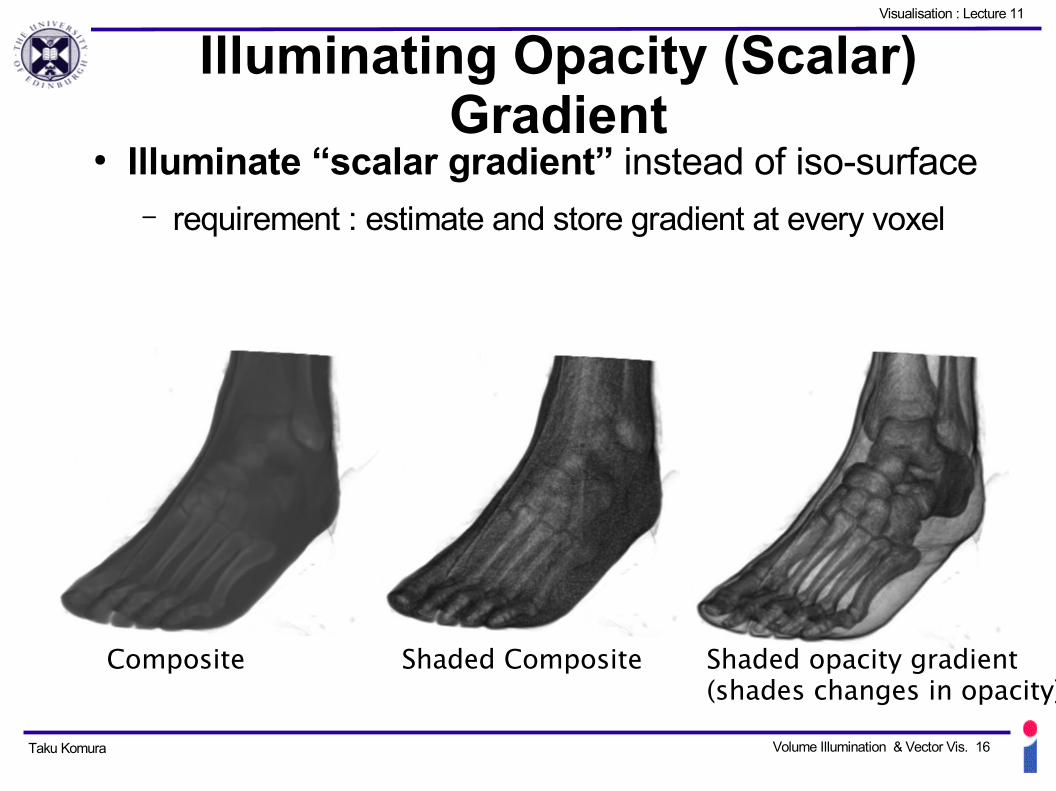
Illuminating Opacity (Scalar) Gradient

● Illuminate “scalar gradient” instead of iso-surface– requirement : estimate and store gradient at every voxel

Composite Shaded Composite Shaded opacity gradient(shades changes in opacity)



Estimating Opacity Gradient

● Use 3D centred difference operator

We can extract the normal vectors of the region where the scalar values are changing significantly, i.e. boundary of tissues

● Evaluate at each voxel and interpolate

∇ I= I x , I y , I z=

xI ,

yI ,

zI

xI=I x1, y , z− I x−1, y , z

2



Illumination : storing normal vectors

● Visualisation is interactive– compute normal vectors for surface/gradient once– store normal– perform interactive shading calculations

● Storage :– 2563 data set of 1-byte scalars ~16Mb – normal vector (stored as floating point(4-byte)) ~ 200Mb!– Solution : quantise direction & magnitude as small

number of bits



Illumination : storing normal vectors

Subdivide an octahedron into a sphere.

Number the vertices.

Encode the direction according the nearest vertex that the vector passes through.

For infinite light sources, only need to calculate the shading values once and store these in a table.

● Quantize vector direction into one of N directions on a sub-divided sphere



Volume Illumination Summary● Illumination can aid visual understanding of volumes

– scattering gives clue to object scale / effects perception— too expensive at current time for interactive visualisation

– Illumination of:— embedded isosurface

– need to estimate surface normal – use depth map— gradient magnitude

– finite difference estimation– Normal vector storage for each cell

— use index into triangulated sphere



Visualising Vectors● Examples of vector data:

– meteorological analyses / simulation– medical blood flow measurement– Computational simulation of flow over aircraft, ships,

submarines etc.– visualisation of derivatives

— not just of flow itself

● Why is visualising these difficult ?– 2 or 3 components per data point, temporal aspects of

vector flow, vector density



Insight in Vector Fields● Two properties of vector fields to visualise :

– local view of the flow– global view of the flow

● e.g a meteorological wind forecast– Local : for given location, what is the current wind strength and

direction

– Global: a given location, where has the wind flow come from, and where will it go to.



Two Methods of Flow Visualisation

● Visualise Flow wrt fixed point– e.g. plot flow glyphs to show local

direction and magnitude– local view of vector field

● Visualise flow as the trajectory of a particles transported by the flow

– e.g plot particle traces, streamlines etc.– global view of vector field– require integrating the flow equation



State of Flow : Steady / Unsteady

● Steady flow – remains constant over time– state of equilibrium or snapshot– use particle traces known as streamlines

● Unsteady flow– varies with time– implications to tracing massless particles– particle traces known as streaklines

— show little information about flow direction or magnitude



Vectors : local visualisation

● Set of basic methods for showing local view:

– oriented lines, hedgehogs & glyphs– colour mapping vector components – warping– animation



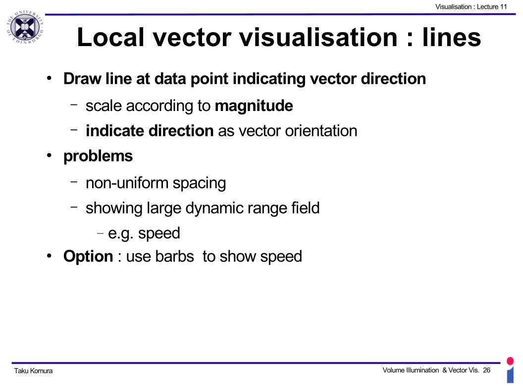
Local vector visualisation : lines● Draw line at data point indicating vector direction

– scale according to magnitude– indicate direction as vector orientation

● problems

– non-uniform spacing– showing large dynamic range field

— e.g. speed● Option : use barbs to show speed



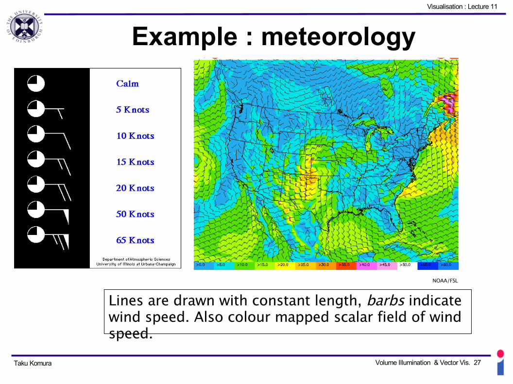
Example : meteorology

Lines are drawn with constant length, barbs indicate wind speed. Also colour mapped scalar field of wind speed.

NOAA/FSL



Example : lines in 3D

● Problems :– Difficult to understand

position and orientation in projection to 2D image.

– Clutter is also a problem.



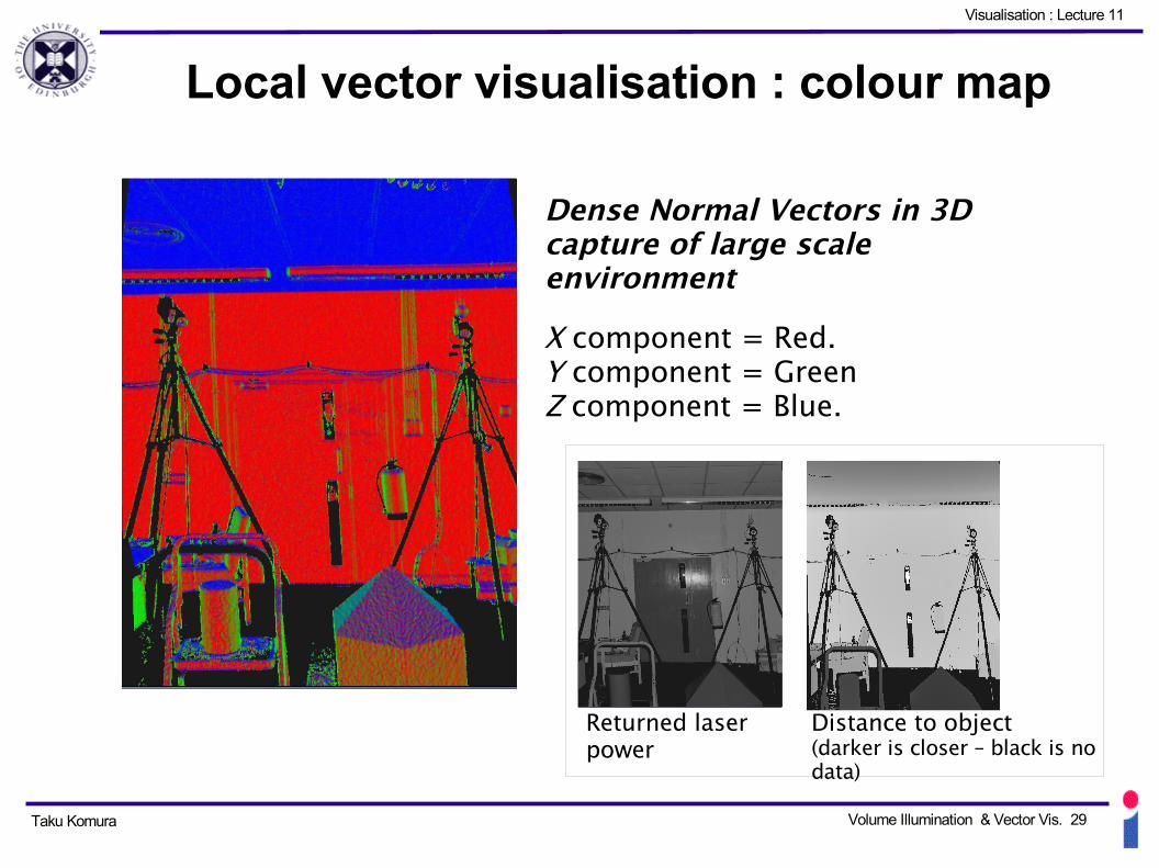
Local vector visualisation : colour map

Dense Normal Vectors in 3D capture of large scale environment

X component = Red.Y component = GreenZ component = Blue.

Returned laser power

Distance to object(darker is closer – black is no data)



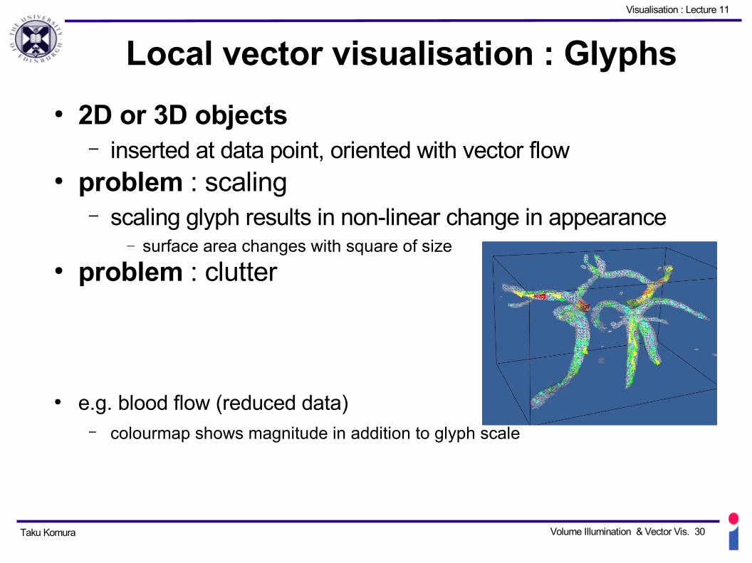
Local vector visualisation : Glyphs

● 2D or 3D objects – inserted at data point, oriented with vector flow

● problem : scaling– scaling glyph results in non-linear change in appearance

— surface area changes with square of size● problem : clutter

● e.g. blood flow (reduced data)– colourmap shows magnitude in addition to glyph scale



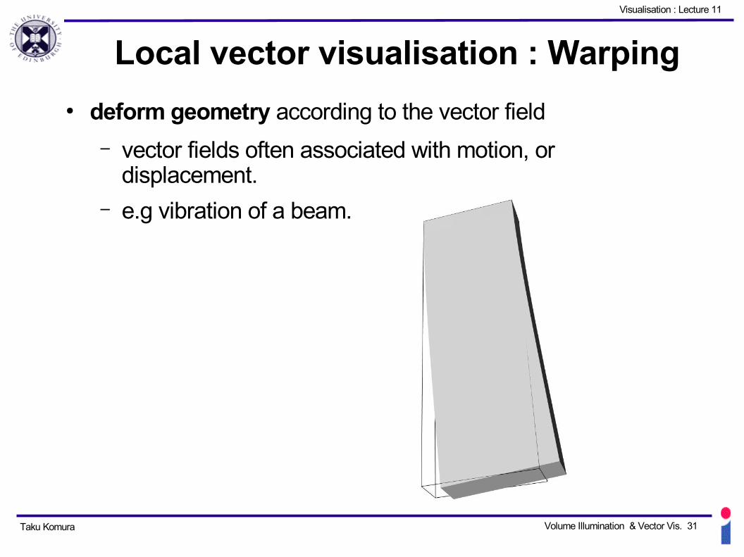
Local vector visualisation : Warping

● deform geometry according to the vector field

– vector fields often associated with motion, or displacement.

– e.g vibration of a beam.



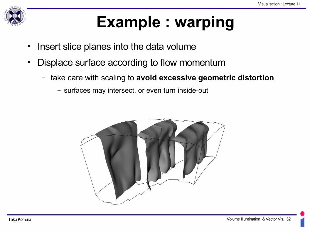
Example : warping● Insert slice planes into the data volume● Displace surface according to flow momentum

– take care with scaling to avoid excessive geometric distortion

— surfaces may intersect, or even turn inside-out



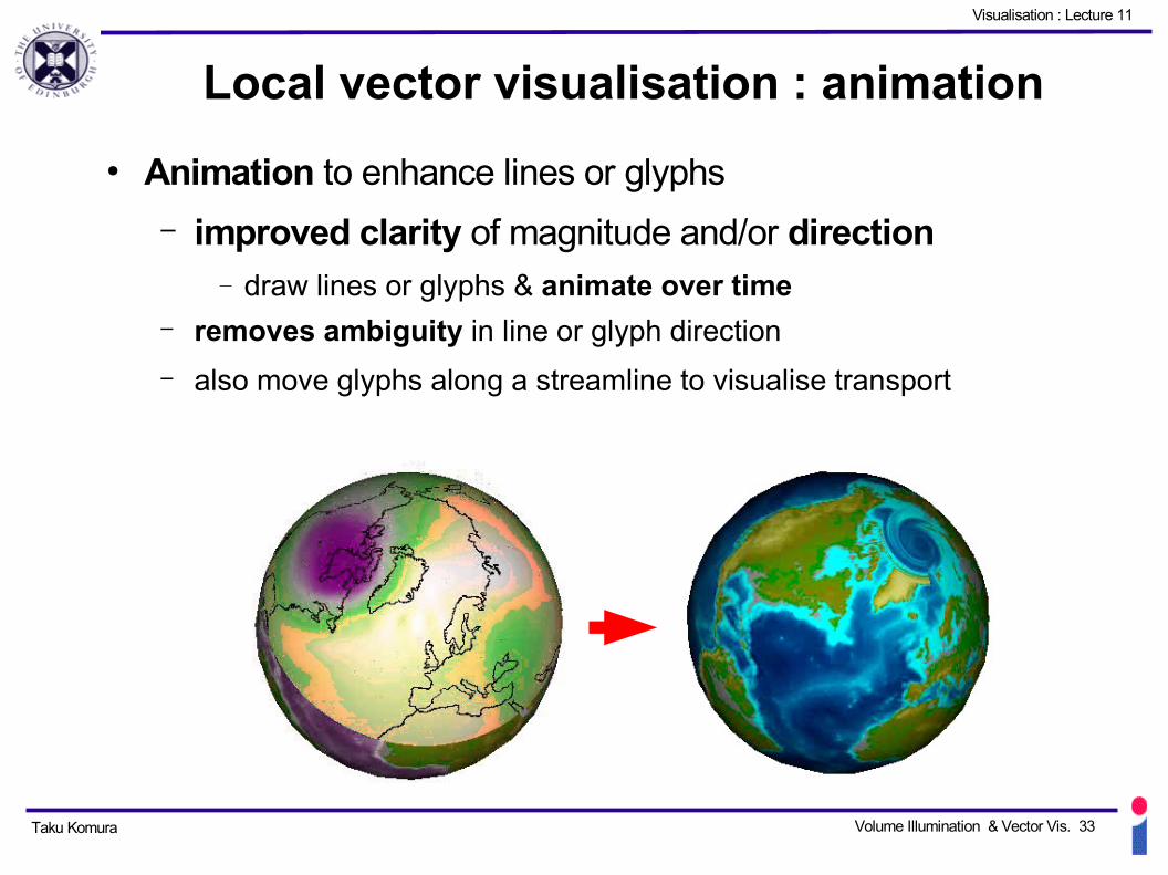
Local vector visualisation : animation

● Animation to enhance lines or glyphs

– improved clarity of magnitude and/or direction— draw lines or glyphs & animate over time

– removes ambiguity in line or glyph direction

– also move glyphs along a streamline to visualise transport



Vector Visualisation Summary● Vector visualisation:

– local view / global view– steady / unsteady flow– methods of vector visualisation :

● Local Vector Visualisation:– lines, hedgehogs & glyphs– colour mapping, warping & animation

Next lecture : more vector fields!

Documents

Volume Illumination & Vector Field Visualisation