Voting in a Multi-dimensional Space: a Conjoint Analysis

1

Voting in a Multi-dimensional Space: a Conjoint Analysis Employing Valence

and Ideology Attributes of Candidates

Fabio Franchino and Francesco Zucchini, Università degli Studi di Milano

Political Science Research and Methods

Valence matters in voting behaviour, but how exactly? A large body of scholarly research

concludes that valence adds a second important dimension to the standard policy-based electoral

competition. Valence issues have the peculiar property of voters having identical preferences over

them. They all prefer more to less of a given valence attribute. They prefer more to less competent

politicians; they prefer more to less honest politicians. Fittingly, Groseclose (2007) argues that

valence adds 'half' a dimension to the standard one-dimensional Downsian model of electoral

competition.

Indeed, most formal models of electoral competition add a single and separable valence component

to the voters’ utility function (e.g. Adams and Merrill III 2009; Ansolabehere and Snyder Jr 2000;

Aragones and Palfrey 2002; Aragones and Palfrey 2004; Castanheira, Crutzen, and Sahuguet 2010;

Groseclose 2001; Londregan and Romer 1993; Schofield 2003; Schofield 2007). The utility of

voter is therefore represented as

( ) (| |)

It is a positive function of the valence of candidate C and a negative function of the difference

between and , the voter’s and the candidate’s positions along a policy dimension, where

and (Groseclose 2001). Voters hold homogeneous views with regard to the valence issue;

and policy and valence dimensions have the same saliency. Variants to this standard approach

include uncertainty over the valence advantage (Adams and Merrill III 2009; Londregan and Romer

1993), multiple policy dimensions and valence traits (Adams et al. 2011; Ansolabehere and Snyder

Jr 2000), as well as different types of politicians (Adams and Merrill III 2009; Groseclose 2001).

brought to you by COREView metadata, citation and similar papers at core.ac.uk

provided by AIR Universita degli studi di Milano

https://core.ac.uk/display/187929583?utm_source=pdf&utm_medium=banner&utm_campaign=pdf-decoration-v1

2

Only Groseclose (2001 appendix B) takes seriously the possibility that policy and valence

components are not separable. Valence may take what he calls, the competency form. He argues:

“suppose valence represents the candidate’s competency for implementing the policy position that

he or she announces. Here, it is reasonable to believe that the voter appreciates a candidate’s

competency more when the candidate has adopted a policy that he or she likes… That is, the

marginal gains from valence is [sic] larger when policy distance is smaller” (882).

These models are designed to produce expectations about the positioning of politicians on the

policy-valence space. Valence plays also a central role in the literature conceiving elections as

screening mechanisms (e.g. Besley and Coate 1997; Caselli and Morelli 2004; Fearon 1999;

Galasso and Nannicini 2011; Mattozzi and Merlo 2008; Messner and Polborn 2004). Galasso and

Nannicini (2011) for instance assume that, in a one dimensional policy space, only centrist voters

care about valence, while extreme voters choose their preferred party, regardless of its valence. This

is equivalent of assuming that voters do not hold homogeneous views about valence, or that only

subset of voters assign to valence a saliency weight strictly greater than zero. More extremely,

Caselli and Morelli (2004) propose a model of citizen-candidates where valence is the only

relevant dimension of competition. These works are primarily concerned with the selection

mechanisms of specific types of low or high valence politicians.

Regardless as to whether the focus is on competition or selection, these models rely on a set of

assumptions about voting behaviour. But how exactly do voters behave in a multi-dimensional

choice setting? How do they choose when confronted with candidates that embody more and less

likable traits? Empirical studies of voting behaviour provide contradicting results. For instance, J.

Green and Hobolt (2008) for Britain and Buttice and Stone (2012) for the US find valence voting to

play a greater role as parties and candidates converge ideologically. Cross-country studies suggest

otherwise. Pardos-Prado (2012) show that the effect of valence on the propensity to vote for a party

increases as ideological polarisation intensifies; similarly, Clark and Leiter (2014) find that valence

3

effects on electoral performance increase as parties diverge from the mean voter’s ideological

position.1

In this article, we employ an experimental technique called conjoint analysis to understand how

voters make decisions when faced with multi-dimensional choices. We have designed a so-called

stated preference experiment where participants are asked to choose between candidates that vary

along three valence (education, income and honesty) and two ideological attributes (attitudes

toward taxation and spending and the rights of same-sex couples). We have administered the

experiment to 347 subjects in 2012-3, resulting in 9,352 votes over pair-wise compared candidates.

Our results indicate that education and integrity, but not income, indeed behave like valence issues

where voters prefer more to less. More interestingly, policy positions and valence attributes are not

separable. They interact, apparently taking the competency form. The impact of higher valence on

the likelihood of voting for a candidate is conditional on such candidate’s policy positions. It is

higher when positions are closer to those of the respondents. Finally, when push comes to shove,

policy trumps valence. Voters are ready to trade a higher valence candidate, with whom they do not

share policy views, for a lower valence one with whom they share such views.

In the next section, we formalize voters’ choice in a multidimensional space employing spatial

voting theory, emphasizing the importance of separable and non-separable preferences and of

1 In an experimental study, Mondak and Huckfeld (2006) find that competence and integrity matter

the most when participants with clear political views evaluate candidates with clear political

affiliations. They matter less if signals about political affiliation are mixed or participants hold

centrist views. However, without measures of participant-candidate ideological proximity, it is hard

to infer whether these results support positive or negative complementarity. Recently, Galeotti and

Zizzo (2014) have analysed the trade-off between competence and trustworthiness of candidates,

showing a slight bias in favour of the latter.

4

saliency of the dimensions. We then introduce the design of the experiment, explain the estimation

model and discuss the main results.

VOTER CHOICE OVER CANDIDATES WITH MULTIPLE ATTRIBUTES

Let { } be a set of candidates, { } a set of attributes, and (

) a -

tuple of values of attribute , where is the th value of attribute and for . is the set

of all attributes’ values and the profile of the cth candidate is denoted by a column vector of

attributes’ values [ ] , where is the value of attribute for candidate c. For

example, there may be three relevant attributes, such as education, integrity and position on taxation

and spending, and each of these attributes can take any of three ordered values. The profile of a

candidate can be characterized by low education, high integrity and a pro-spending position.

The ideal candidate of a respondent is represented by the column vector [ ] , where

is her ideal value of attribute and . In a pairwise comparison of candidates’ profiles

(i.e. ), let ( ) { } be the potential binary outcome of respondent over a candidate

with profile . The value of 1 represents that the respondent would choose the cth profile if she got

the treatment , while the value of 0 means that she would not choose such profile. Since

respondents must choose one profile in each decision, ∑ ( ) for . Employing the

weighted Euclidean distance of spatial voting theory (Enelow and Hinich 1984; Hinich and Munger

1997: 80), we have therefore,

( ) iff [( ) ( )]

⁄ [( )

( )]

⁄ ,

where is a symmetric positive-definite matrix of order .2 The diagonal elements in measure

the salience attached by respondent to each attribute, and the off-diagonal elements capture the

interaction across attributes. If is an identity matrix, respondent attaches the same weight to

2 In case of equivalence, the respondent is indifferent between the two candidates and we assume

that she flips a coin.

5

each attribute and preferences are separable across attributes. If the diagonal elements in take

difference values, the respondent assigns more salience to some attributes in her voting decision.

For instance, she may consider a candidate’s integrity more important than his income. In a

bidimensional space, indifference contours take an elliptical rather than a circular shape. If the off-

diagonal elements in are different from zero, preferences are nonseparable and attributes interact

along the lines of the competency form discussed by Groseclose (2001). Attributes can be positive

(negative) complements if a higher level of one attribute makes a respondent wanting more (less) of

another attributes.3 For instance, a voter may value a candidate’s level of education more when the

candidate shares the voter’s opinions on policy. If a candidate’s reputation is tainted, she may

display more conservative attitudes on taxation and spending.

A CONJOINT ANALYSIS VOTING EXPERIMENT

Conjoint analysis is a method that allows isolating the aspects that influence a respondent’s choice

in a multidimensional space. It originates from mathematical psychology (Luce and Tukey 1964)

and it has been extensively employed in marketing research and economics to measure consumer

preference, forecast demand and develop new products (P. E. Green and Rao 1971; P. E. Green,

Krieger, and Wind 2001; Hensher, Rose, and Greene 2005; Raghavarao, Wiley, and Chitturi 2010).

3 Take the case of two attributes, the weighted Euclidean distance (WED) is ( )

( )( ) ( ) , where and are respectively the ideal and

candidate values and the salience weight of attribute , while the interaction between the

attributes (the off-diagonal element in ). Since ( )⁄ ( )

( ) , the marginal effect of the difference between the ideal and candidate values along

attribute 1 is also a function of such difference in attribute 2 and of the sign of the interaction term

. The spatial model cannot not capture the possibility that sets of attributes may be nonseparable

from other sets of attributes (Lacy 2001, 240).

6

It has been applied only very recently to research questions in political science (Hainmueller and

Hopkins 2012; Hainmueller, Hopkins, and Yamamoto 2014).

We have designed a conjoint analysis voting experiment to assess how attributes of candidates,

related to valence and ideology, affect voters’ choice. Respondents are subject to choice tasks

where they have to choose between two generically labelled candidates A and B.4 These candidates

are characterised by five attributes and each attribute takes one of three values, that is, { },

{ } and (

) where .

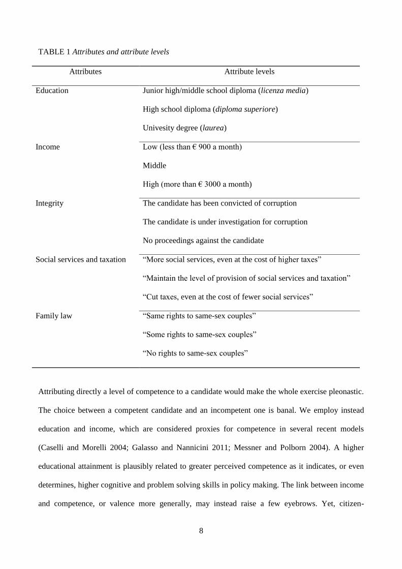
The five attributes and their values are described in Table 1; three are meant to be related to

valence, two to ideology or policy. Following Stokes (1963) seminal contribution, the literature

offers a long list of possible valence factors, from the strength of the economy (e.g. Anderson 2000;

Butler and Stokes 1969; Fiorina 1977; Lewis-Beck, Nadeau, and Elias 2008; Palmer and Whitten

2000), to issue ownership (e.g. Budge and Farlie 1983; Bélanger and Meguid 2008; Clarke et al.

2004; J. Green and Hobolt 2008), party unity (Clark 2009), incumbency, name recognition and

campaigning skills (e.g. Adams et al. 2011; Enelow and Hinich 1982; Fiorina 1981; Groseclose

2001; Londregan and Romer 1993; Stone and Simas 2010). These factors are not particularly

meaningful or useful in pairwise comparisons between generically labelled candidates. They are

either context-specific or instrumental – and the latter are not valued intrinsically by voters. In light

4 Like Hainmueller, Hopkins and Yamamoto (2014), we exclude party labels because the opinions

participants have with regard to a given party may either be correlated with existing attributes or be

proxies for omitted ones, therefore confounding our analysis of how respondents trade between

policy and valence. With generic labels, the unobserved components of the choice function are less

likely to be cross-correlated and more likely to have the same distribution (Hensher, Rose, and

Greene 2005, 112–3). The design of the experiment is also simplified because otherwise you would

need several party labels and more tasks. The downside is that we cannot test the impact of party

identification.

7

of the models reviewed above, we are interested in candidate-specific and character-based attributes

related competence and integrity (e.g. Adams et al. 2011; Clark 2009; Clark and Leiter 2014; Funk

1996; Funk 1999; Kulisheck and Mondak 1996; McCurley and Mondak 1995; Mondak and

Huckfeldt 2006; Stone and Simas 2010).

8

TABLE 1 Attributes and attribute levels

Attributes Attribute levels

Education Junior high/middle school diploma (licenza media)

High school diploma (diploma superiore)

Univesity degree (laurea)

Income

Low (less than € 900 a month)

Middle

High (more than € 3000 a month)

Integrity The candidate has been convicted of corruption

The candidate is under investigation for corruption

No proceedings against the candidate

Social services and taxation “More social services, even at the cost of higher taxes”

“Maintain the level of provision of social services and taxation”

“Cut taxes, even at the cost of fewer social services”

Family law “Same rights to same-sex couples”

“Some rights to same-sex couples”

“No rights to same-sex couples”

Attributing directly a level of competence to a candidate would make the whole exercise pleonastic.

The choice between a competent candidate and an incompetent one is banal. We employ instead

education and income, which are considered proxies for competence in several recent models

(Caselli and Morelli 2004; Galasso and Nannicini 2011; Messner and Polborn 2004). A higher

educational attainment is plausibly related to greater perceived competence as it indicates, or even

determines, higher cognitive and problem solving skills in policy making. The link between income

and competence, or valence more generally, may instead raise a few eyebrows. Yet, citizen-

http://www.lasir.net/onlinesurvey/attributes.jsp?action=remove_attrib&attributeID=1

http://www.lasir.net/onlinesurvey/attributes.jsp?action=remove_level&attributeID=1&levelID=0



9

candidate models, which seek to fully endogenize candidacies by removing the distinction between

the electorate and the political class and are particularly concerned with the qualities of politicians

(Dewan and Shepsle 2011), unabashedly assign to income a strong connotation of valence as “a

measure of market success and ability” (Galasso and Nannicini 2011, 79). For Caselli and Morelli

(2004, 775), “voters use [candidates’] market incomes as a signal of their competence” in office. On

the other hand, income may signal other features, such as class membership, and therefore display

no valence behaviour. Our experiment will subject these assertions to testing.

The education attribute includes three levels of attainment: junior high school diploma, high school

diploma and university degree. In Italy, they are called licenza media, diploma superiore and

laurea. The levels of income are low, medium and high. Low income is specified as below €900 a

month, which is approximately the second decile of the 2009 income distribution in Italy. High

income is specified as above €3000 a month, approximately the ninety-fifth percentile.5

As far as the third valence attribute is concerned, it is introduced as additional information, thus

avoiding more laden terms such as integrity. A candidate may have been convicted of corruption, be

under investigation for corruption or have a clean sheet - corruption being the most common office-

related crime a politician is likely to be charged with.

Candidates also differentiate along policy positions which are derived from well-established

cleavages: the liberal-interventionist economic divide and liberal-conservative social one (e.g.

Benoit and Laver 2006: 160; Kitschelt 1994). To capture the former, we established that candidates

may want to increase the provision of social services, even at the cost of more taxation, to maintain

the current levels, or to cut taxes, even at the cost of fewer social services. These are frequently the

top priorities of government for Italian public opinion (European Commission 2010: 24). For the

latter, candidates may want to grant no family-related rights to same-sex couples, to grant these

couples some rights or even the same rights as traditional families. This is currently the most

5 Eurostat dataset on the distribution of income by quantiles in 2009, source: SILC.

10

debated issue that captures the liberal-conservative social divide in Italy. Others, such as abortion

and euthanasia, are less prominent.

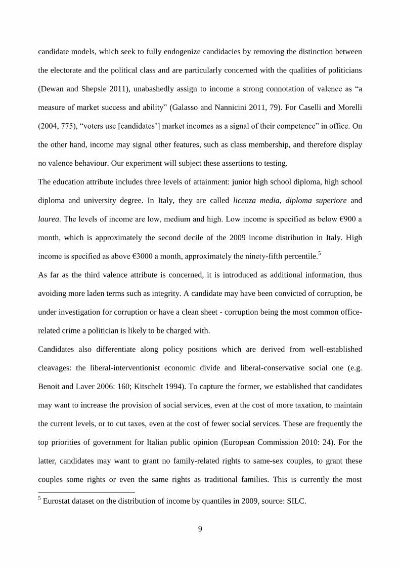
TABLE 2 Example of a choice task

Question: For whom would you vote?

Candidate A Candidate B

Education High school diploma High school diploma

Income

High (more than € 3000 a

month)

Middle

Other information

The candidate is under

investigation for corruption

The candidate is under

investigation for corruption

Opinion on social services and

taxation

More social services, even at

the cost of higher taxes

Cut taxes, even at the cost of

fewer social services

Opinion on family law

Some rights to same-sex

couples

Same rights to same-sex

couples

Table 2 illustrates an example of a choice task. Note that it does not offer the possibility of

abstention. Although including this option would better reflect the situation in which voters find

themselves, we are not interested in participation in this context. Our objective is to assess the

impact of candidates’ attributes on voters’ choice. A no vote alternative is a hindrance for our

analysis because the only information that can be derived from abstention is that the respondent

would prefer not to choose. We do not obtain any information of why this is so. As Hensher, Rose

and Greene (2005: 176) argue, ‘by forcing decision makers to make a choice, we oblige decision

makers to trade off the attribute levels of the available alternatives and thus obtain information on

the relationships that exist between the varying attribute levels and choice’.

11

Experimental Design Considerations

Which candidate profiles should be included in the conjoint analysis and how should be paired? A

full factorial design is one in which all possible treatment combinations (i.e. profiles) are

enumerated (Hensher, Rose, and Greene 2005: 109). With five attributes and three levels per

attribute, we have 243 (i.e. ) different profiles. Since we ask respondents to pairwise compare

candidates, the full enumeration of choice tasks amounts to 29,403, that is(

), combinations.

Such a design is clearly unfeasible. We will therefore use only a fraction of these combinations – a

so-called fractional factorial design.

The minimum number of profiles of a fractional factorial design is determined by the degrees of

freedom we need for the subsequent model estimation. Since the alternative candidates are

unlabelled, the estimation of the main effects of five attributes requires at least six degrees of

freedom for a linear model and, because each attribute takes three values, at least eleven degrees for

a non-linear model. Moreover, testing the competency form entails interactions. The addition of an

interaction between two attributes requires the estimation of one more parameter in case of a linear

model and four more parameters in case of a non-linear model. In other words, if we want to

estimate the main effects and, say, two interactions, we need at least eight degrees of freedom for a

linear model and nineteen degrees for a non-linear model.

Additionally, a statistically efficient fractional factorial design must be orthogonal, where columns

display zero correlation (Hensher, Rose, and Greene 2005: 115). In other words, the levels that an

attribute takes across all choice tasks should be statistically independent from the levels other

attributes take. Orthogonality may demand a number of combinations that exceeds the minimum

requirement imposed by the degrees of freedom (in our case, nineteen for a non-linear model).

However, for unlabelled designs, only within-alternative orthogonality needs to be maintained

(Hensher, Rose, and Greene 2005: 152). In other words, the education attribute of candidate A

across all the choice tasks does not need to be orthogonal to the education attribute of candidate B.

12

A last appreciable feature is that the design should be balanced. Each level of any given attribute

should appear the same number of times.

Since we require only within-alternative orthogonality, we generated a main-effects orthogonal

design for five attributes and three levels for attribute, setting at twenty-seven the minimum number

of cases (rows). The design is balanced because each level of each attribute appears nine times. We

have assigned attributes to the columns of the design in order to ensure statistically efficient

estimations of the main effects and of the interactions between education and the two policy

dimensions (for the details on the procedure see Hensher, Rose, and Greene 2005: 127-150). Seven

out of the possible ten two-way interactions between attributes display zero correlation with the

main effects. Several interactive terms are also uncorrelated with each other. In practise, this means

that we can efficiently estimate the marginal effects of all the ten pairwise interactions among the

five attributes.6 We have now twenty-seven orthogonal profiles of candidate A. We have then

randomized the sequence of these profiles and assigned them to candidate B, making sure that the

randomized combination does not match the original. This procedure ensures within-alternative

orthogonality (Hensher, Rose, and Greene 2005: 152).

The core of the experiment consists in twenty-seven choice tasks (i.e. ) where respondents

are requested to choose between two candidates’ profiles. The order of the attributes, as it appears

in Table 2, does not change for each respondent in order to ease the cognitive burden, but the

6 The fractional factorial and orthogonal design is the most widely used in the conjoint analysis

literature. In introducing this method to political science, Hainmueller, Hopkins and Yamamoto

(2014) recently proposed a randomized variant of conjoint analysis that does not require any

assumption about choice probabilities. Our design imposes no restrictions to the pairwise

interactions and to five of the six three-way interactions. Of the interaction between income,

integrity and family law, only the following profiles are observed: middle income, corrupt and some

rights; high income, investigated and some rights; high income, corrupt, no rights.

13

sequence of tasks is randomized across respondents in order to minimise primacy and recency

effects.

The only applications of conjoint analysis in political science is in the field of public opinion

(Hainmueller and Hopkins 2012; Hainmueller, Hopkins, and Yamamoto 2014). In light of the

formal literature reviewed above, our interest is more circumscribed. We want to analyze how

respondents reconcile valence and policy features of candidates in their voting choices. We are less

interested in how different types of respondents prefer different candidates, although trade-offs may

differ across types. Given the nature of our inquiry, a set of relatively homogeneous respondents

allows us to better control for unobservables that may confound the interaction between attributes

(Hensher, Rose, and Greene 2005). We have therefore involved 155 undergraduate students in the

period between February and May 2012, and then repeated the exercise with further 192 students

between January and May 2013. The experiment, structured as an online survey, has been

administered by the Opinion Polls Laboratory (Laboratorio Indagini Demoscopiche) of the

Università degli Studi di Milano. Clearly, our results are not generalizable to a wider population,

but we are nevertheless able to highlight similarities with recent public opinion studies

(Hainmueller, Hopkins, and Yamamoto 2014). Future research should consider the development of

a representative online sample for further corroborating these findings.

ESTIMATION

To estimate how attributes of candidates influence the choice of respondents, we employ a binomial

model with a conditional logit link function. Voting is assumed to be generated by a Bernoulli

process. The stochastic component of the model is therefore ( | ), where

( | ) for respondent and candidate . The systematic component is

[(∑ ) ( ) ]

∑ [∑ ) ( ) ]

(1)

where is the value of attribute for candidate c, with the interactions between education ( )

and the two policy dimensions ( ), is the Hadamard product of row vectors of betas

14

and socio-demographic and political characteristics7 of the respondent , while is the column

vector of attributes of candidates. Respondent characteristics must interact with candidate attributes

because they do not display within-group variance, i.e. they do not vary across profiles.

VALENCE, IDEOLOGY AND VOTING

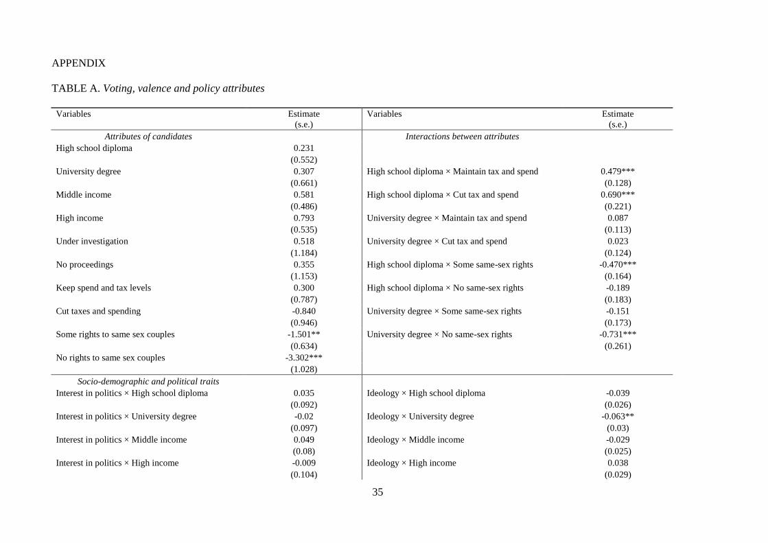
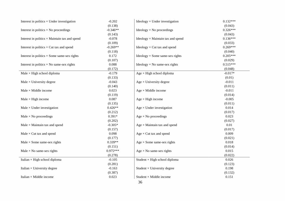
The results of the estimation are reported in the Appendix (Table A). In this section, we first assess

whether the attributes we selected behave as expected. Next, we evaluate whether the preferences of

respondents take the competency form. Finally, we analyze how respondents trade off profiles of

candidates in their voting decisions. The online appendix includes diagnostic tests.

The Behavior of Valence and Policy Attributes in Voting Decisions

Do the first three attributes indeed behave like valence issues where voters prefer more to less? Do

the last two attributes display the features of policy issues that split voters in different groups? In

other words, do the core assumptions underpinning formal models of policy-valence based electoral

competition hold? Are the measures of valence used in recent formal and empirical analyses valid?

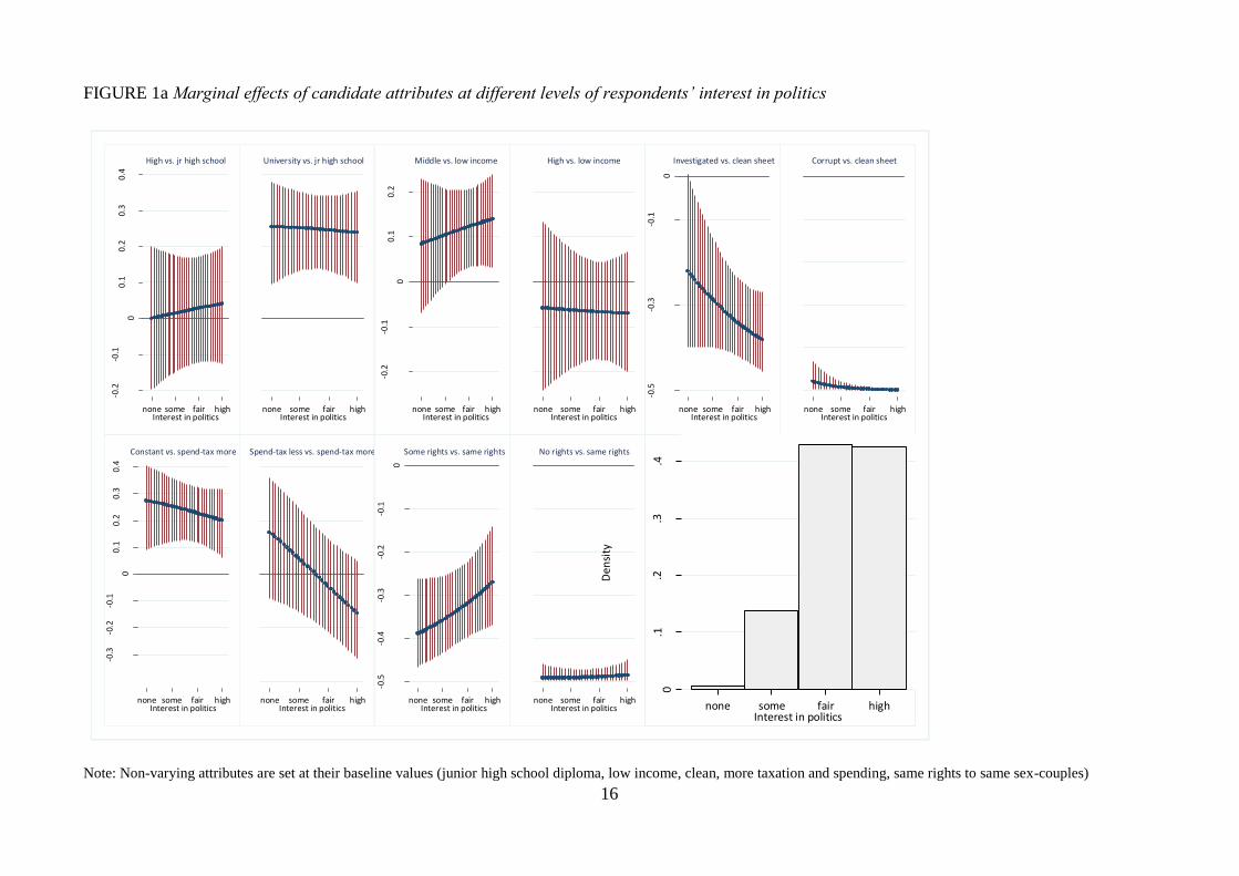
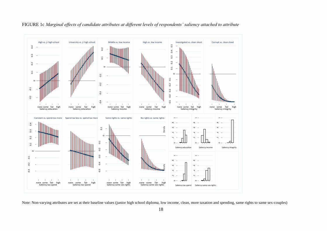
Figures 1a to 1c display the marginal effects of different attributes on the probability that

respondents vote for a particular candidate, at different levels of respondents’ interest in politics,

left-right self-placement and issue saliency (see the online appendix for similar figures on the

remaining traits).8 For instance, the upper-left panel in Figure 1a displays on the vertical axis the

7 As socio-demographic traits, we include gender, age, nationality, working status and high school

education; as political traits, interest in politics, left-right self-placement, and saliency attached to

attributes. Lastly, we include an indicator variable for respondents participating in 2013.

8 Marginal effect plots are produced following Brambor, Clark and Golder (2006) and the STATA

code available at https://files.nyu.edu/mrg217/public/interaction.html#code. These effects are

bounded between -0.5 and 0.5 because we set the non-varying attributes at the baseline levels. Had

we set them at different levels, the effects would have been confounded by the interactions between

15

marginal effect on the probability that respondents vote for a candidate with a high school diploma,

compared to one with a junior high school diploma, at different levels of interest in politics declared

by the respondents. The dots indicate the mean predicted probabilities and the lines the 95%

confidence intervals. The bottom right panel is a histogram of respondents’ traits.

respondent characteristics and such attributes. The asymmetric confidence intervals in Figure 3 and

Figures A6 to A9 in the online appendix result from the interactions among profile attribute levels.

16

FIGURE 1a Marginal effects of candidate attributes at different levels of respondents’ interest in politics

Note: Non-varying attributes are set at their baseline values (junior high school diploma, low income, clean, more taxation and spending, same rights to same sex-couples)

-0.2

-0.1

00.

10.

20.

30.

4

none some fair highInterest in politics

High vs. jr high school


University vs. jr high school

0.2

0.1

0

-0.1

-0.2


Middle vs. low income


High vs. low income

0

-0.1

-0.3

-0.5


Investigated vs. clean sheet


Corrupt vs. clean sheet

0.4

0.3

0.2

0.1

0

-0.1

-0.2

-0.3


Constant vs. spend-tax more


Spend-tax less vs. spend-tax more

0

-0.1

-0.2

-0.3

-0.4

-0.5


Some rights vs. same rights


No rights vs. same rights

0.1

.2.3

.4

Den

sity


17

FIGURE 1b Marginal effects of candidate attributes at respondents’ different left-right self-placements


-0.2

-0.1

00.

10.

20.

30.

4

left center rightIdeology




-0.2

-0.1

00.

10.

20.

3




High vs. low income

-0.5

0.4

-0.3

-0.2

-0.1

00.

1





-0.4

-0.3

-0.2

-0.1

000.

10.

20.

30.

40.

5





-0.5

-0.4

-0.3

-0.2

-0.1

00.

10.

20.

30.

4





0

.05

.1.1

5.2

.25

Den

sity


18

FIGURE 1c Marginal effects of candidate attributes at different levels of respondents’ saliency attached to attribute


-0.2

-0.1

00.

10.

20.

30.

4

none some fair highSaliency education


none some fair highSaliency education


0.2

0.1

0

-0.1

-0.2

-0.3

-0.4

none some fair highSaliency income


none some fair highSaliency income

High vs. low income

0.5

0.4

0.3

0.2

0.1

0

-0.1

-0.2

-0.3

-0.4

-0.5

none some fair highSaliency integrity


none some fair highSaliency integrity


0.4

0.3

0.2

0.1

0

-0.1

-0.2

-0.3

none some fair highSaliency tax-spend


none some fair highSaliency tax-spend


0.1

0

-0.1

-0.2

-0.3

-0.4

-0.5

none some fair highSaliency same-sex rights


none some fair highSaliency same-sex rights


0.2

.4.6

.81

Den

sity

Saliency education

0.2

.4.6

.81

Saliency income

0.2

.4.6

.81

Saliency integrity

0.2

.4.6

.81

Den

sity

Saliency tax-spend

0.2

.4.6

.81

Saliency same-sex rights

19

To a large extent, education behaves like a valence attribute. For almost any respondent trait, a

university educated candidate is significantly more likely to be preferred over a candidate with only

a junior high school diploma. For instance, assuming intermediate values for other traits,9

respondents are between 23.8 and 25.5 percentage points more likely to choose the former profile,

for any level of declared interest in politics (with 95% confidence intervals ranging from 9.7 to 37.9

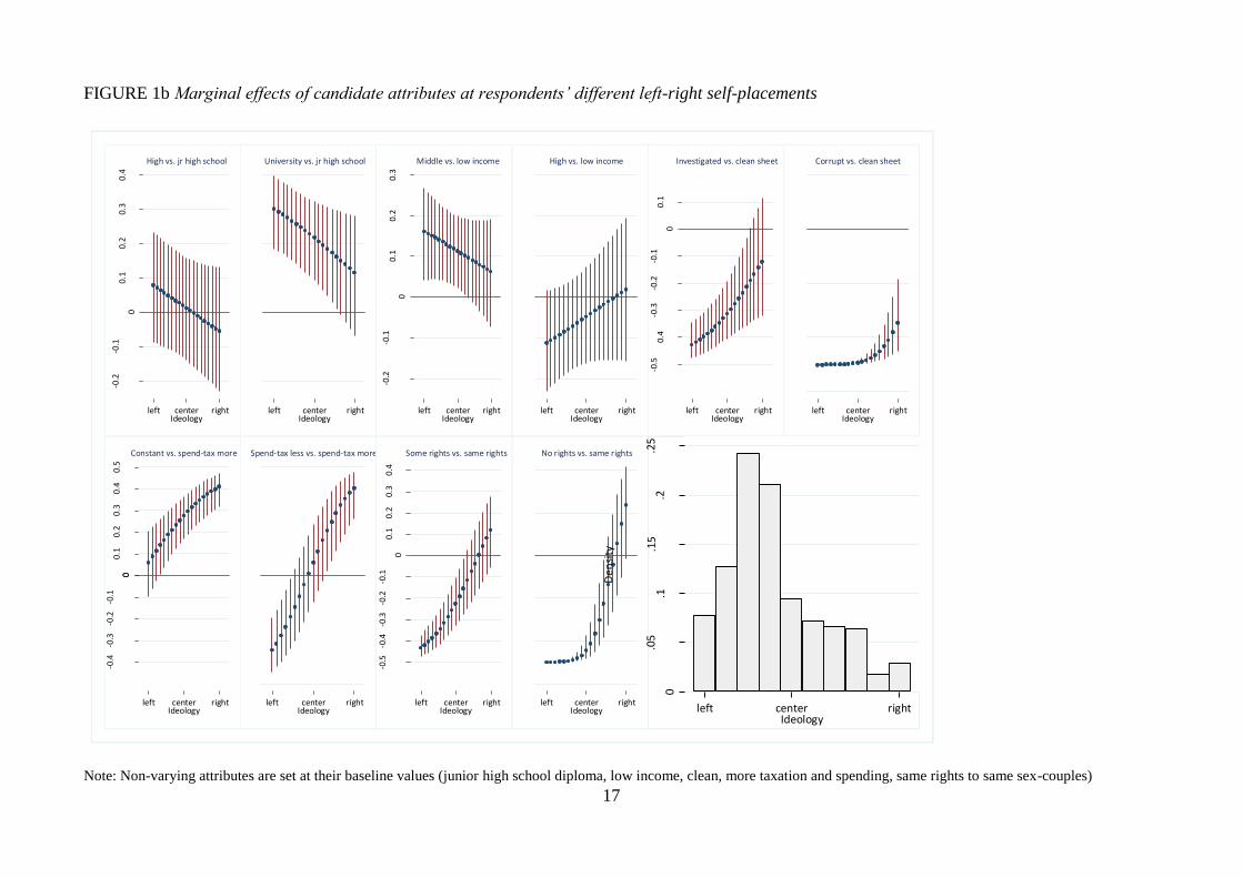
percentage points). Right, center or left-leaning respondents are between 16.2 and 30.2 percentage

points more likely to support such a candidate, with estimates ranging between 1.1 and 39.7 points.

If education is considered an important attribute, a candidate with a university degree is between

23.2 and 33.5 percentage points more likely to win support, with the estimate ranging between 11.1

and 41.5 points. Yet, there are some nuances. Better educated candidates are not significantly

preferred over less educated ones by respondents that are either strongly right-leaning or attach

limited importance to education. These subjects make up 22.8 percent of the respondent pool.

Nevertheless, like in the candidate experiment of Hainmueller, Hopkins and Yamamoto (2014), the

overall valence features of education are evident.

The same cannot be said for income. Middle income candidates are slightly advantaged over low

income ones, especially if respondents are left-leaning and interested in politics.10

But, noticeably,

this is also true for subjects that attach limited relevance to this attribute. More importantly, rich

candidates are not significantly preferred over poor ones, for any respondent trait. If anything, high

income is a liability rather than an asset. Respondents that attribute fair or high importance to

income are between 18.9 and 28.2 percentage points less likely to prefer a rich over a poor

candidate. These results resonate well with those of Hainmueller, Hopkins and Yamamoto (2014)

where middle-income matters, slightly, to win contests but high-income candidates are rated lower.

9 In computing marginal effects, we keep the respondents’ socio-demographic and political traits,

which are not object to analysis, to their mean or modal values.

10 Full time students and Italian nationals also display this behaviour.

20

Far from being an indicator of ability, or even competence in office (cf. Caselli and Morelli 2004,

775; Galasso and Nannicini 2011, 79), high income is seen quite suspiciously by our respondents.11

The last, somewhat obvious, result is that the valence behavior of the integrity attribute is beyond

doubt. For any respondent trait, a clean candidate is significantly more likely to be preferred over a

corrupt one. Even nuances are quite minor. Respondents, which are either strongly right-leaning or

display no interest in politics,12

are indifferent between candidates that are clean and those that are

under investigation, but these subjects make up only 9.5 percent of the respondent pool.

Contrast this with the opinions of candidates on spending and taxation. Figure 1b illustrates that

respondents are neatly split along the left-right axis. A candidate proposing to cut spending and

taxation is 34.6 percentage points less likely to win support from a left-wing respondent and 40.3

percentage points more likely to win support from a right-wing respondent, than a candidate

proposing more spending and taxation. Consequently, moderately positioned candidates are favored

over extremely positioned ones for most values of respondent traits, of course, with the exception of

strongly left- or right-leaning subjects.

The issue of rights for same-sex couples behaves in a similar way, though less neatly. A candidate

arguing for no rights to same-sex couples is 50 percentage points less likely to win support from a

left-wing respondent and 23.4 percentage points more likely to win support from a right-wing

respondent, than a candidate proposing the same rights as traditional families (the latter value is

significant at the 90 percent confidence interval). Still, for most values of respondent traits, except

ideology, candidates arguing for equality of treatment are preferred to candidates willing to

recognize only some rights. The young age of the respondents mostly likely explains these liberal

views (e.g. Bartels 2013). Having established the valence behavior of education and integrity and

11

Moreover, candidates that have high income and are corrupt face the harshest penalties.

12 Non-Italian respondents as well.

21

the policy behavior of the positions on taxation and spending and on the rights of same-sex couples,

we move on to analyze how participants trade-off between these attributes.

Evidence of a Competency Form: Interaction among Education and Policy Attributes

Is it plausible to assume that valence is a separable component that is simply added to a standard

policy-based dimension as most formal models of electoral competition do? Or do valence and

policy attribute interact, perhaps taking what Groseclose (2001) calls a competency form? In other

words, do voters attach less value to valence when a candidate’s policy position differs from their

own?

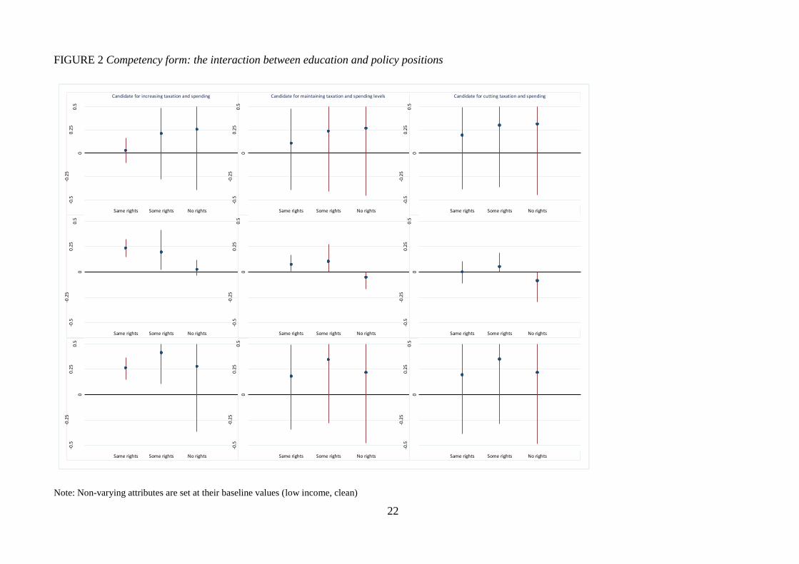
Figure 2 illustrates the marginal effects of different levels of educational attainment, our proxy for

competence, on the probability that a typical respondent13

votes for a particular candidate policy

profile (the online appendix includes the complementary Figures A4 and A5 on the marginal effects

of policy positions). For instance, the top three panels display the marginal effects on the

probability that a typical respondent votes for a candidate with a high school diploma, compared to

one with a junior high school diploma, across the nine combinations of policy profiles. In this case,

higher education does not have much of an effect.

13

Our typical respondent is an Italian female full-time student with a fair interest in politics and

left-of-center views. She is twenty-one years old, comes from a lyceum and attaches high saliency

to the integrity and spending dimensions, fair saliency to education and couples’ rights, and some

importance to income.

22

FIGURE 2 Competency form: the interaction between education and policy positions

Note: Non-varying attributes are set at their baseline values (low income, clean)

0.5

0.25

0

-0.2

5-0

.5

Hig

h v

s jr

hig

h sc

hoo

l

Same rights Some rights No rights

Candidate for increasing taxation and spending

0.5

0.25

0

-0.2

5-0

.5


Candidate for maintaining taxation and spending levels

0.5

0.25

0

-0.2

5-0

.5


Candidate for cutting taxation and spending

0.5

0.25

0

-0.2

5-0

.5

Uni

vers

ity

vs h

igh

sch

ool


0.5

0.25

0

-0.2

5-0

.5


0.5

0.25

0

-0.2

5-0

.5


0.5

0.25

0

-0.2

5-0

.5

Uni

vers

ity

vs jr

hig

h s

cho

ol


0.5

0.25

0

-0.2

5-0

.5


0.5

0.25

0

-0.2

5-0

.5


23

Consider now the left panels in the second and third rows of Figure 2. Candidates, who support

spending and at least some rights for same-sex couples, are between 20 and 23.4 percentage points

more likely to be chosen if they have a university degree, rather than a high school diploma. These

figures increase to 26.4 and 42.6 points respectively when university education is compared to a

junior high school diploma. Conversely, if a candidate opposes the recognition of rights to same-sex

couples, there is no level of education that is going to make him more palatable. This policy is

strongly opposed by our typical respondent. Hence, the marginal gains from higher education

vanish when policy distance increases – the key trait of Groseclose’s (2001) competency form.

As the right panel in the second row of Figure 2 illustrates, higher education can even become a

liability. A university educated candidate is 9.5 percentage points less likely to be chosen than a

candidate with a high school diploma if, in addition to opposing rights for same-sex couples, he

supports spending cuts as well (the estimate varies between 31 and 0.04 points). These two

positions are strongly disliked by our typical respondent14

and higher competence is actually

perceived as worrisome in this case.

For intermediate profiles, our typical respondent trades between candidate attributes depending on

their levels. Consider a candidate supporting full recognition of rights (left column of Figure A4). If

he opposes spending, higher education does not increase his chances of being selected. If he

supports cuts, and he is poorly educated, he is between 30.9 and 35.4 percentage points less likely

to be chosen than a pro-spending or pro-status quo candidate.

Take now a candidate supporting partial recognition. In case of a status-quo position on spending, a

university education gives a candidate a 10.9 percentage point increase in the likelihood of being

preferred compared to a high school diploma (centre panel in Figure 2). In case of a pro-cuts

14

There is no level of education (or stance on the rights issue) that makes a pro-cuts candidate more

appealing than a pro-status quo one (bottom row of Figure A4), and a no-rights position is

comprehensively penalized (second and third rows of Figure A5).

24

position, a university education gives a 40.9 percentage point increase compared to a junior high

school diploma (right panel in the third row).

In other words, the preferences of our typical respondents are finely balanced with intermediate

profiles. If a candidate is for partial recognition but has only a junior high school diploma, a pro-

status quo fiscal attitude makes him 35.3 percentage points more likely to be chosen than a

spendthrift one (top row of Figure A4). Poor education makes our respondents wary of profligacy.

But this does not extend necessarily to rights issues. If a candidate is pro-spending but poorly

educated, a full-recognition stance makes him still 15.5 percentage points more likely to be chosen

than a partial-recognition position (top row of Figure A5).

The trade-offs can indeed get quite complicated to understand in these intermediate profiles.

Nevertheless, what is important to take away from this section are the significant interactions

between valence and policy attributes as envisaged by Groseclose’s (2001) competency form. This

emerges more clearly on the dimension of same-sex couple rights. An F-test for the joint

significance of the interaction terms rejects the null hypothesis that the effects of university

education are identical across attribute levels (p-value ≈ 0.003). Moreover, the null hypothesis

cannot be rejected when comparing candidates that support full and partial recognition (p-value ≈

0.38), while it is easily rejected when comparing candidates that support full and no recognition (p-

value ≈ 0.005). These results appear to indicate positive complementarity, in line with the findings

of J. Green and Hobolt (2008) and Buttice and Stone (2012). On the spending dimension, since

respondents hold a moderate position, this dynamics does not emerge as clearly.

However, which attributes ultimately prevail when respondents are confronted with awkward

choices? We move to this question in the next section where we finally pull in integrity - the

archetypal valence attribute.

25

Policy Trumping Valence in Awkward Choices

Candidates with dubious traits frequently run at the elections, and win. In citizen-candidates

models, this outcome results from an oversupply of low-quality candidates due to limited electoral

competition or a failure to coordinate by high-quality citizens (e.g. Caselli and Morelli 2004;

Myerson 1993). The ideal candidate of our typical respondent has indeed a university education and

a clean sheet, though, notice, only a middle income. Respondents also typically prefer full

recognition of rights and oppose spending cuts. This candidate profile trumps over all the

alternatives,15

but are respondents more likely to sacrifice valence or policy attributes when

confronted with awkward choices? How do voters choose if a high quality candidate is on offer, but

his policy views are far from their ideal?

Figure 3 lists, on the left-hand side, profiles of candidates supporting full recognition of rights and

opposing spending cuts, but falling short in terms of valence. Their educational attainment is lower

or there are issues concerning their integrity. The candidates on the right-hand side are university

educated and honest, but they are pro-cuts and against the recognition of rights. Figure 3 displays

the marginal effects of choosing the latter candidates, given the former; in other words, the changes

in the probability of preferring a high valence candidate with different policy views over a lower

valence candidate with ideal policy views. If the marginal effect is lower (higher) than zero,

respondents are less (more) likely to prefer the higher valence candidate.

15

More precisely, the typical respondent is significantly more likely to prefer a profile with these

traits over one with at least one different trait - with one small caveat. Keeping constant the other

ideal traits, a university educated candidate is preferred to one with a high school diploma only at a

90 percent confidence interval. Note that the typical respondent is indifferent between a pro-status

quo and a pro-spending candidate. These policy positions resonate well with Bartels’ (2013)

analysis, considering the young age of the respondents.

26

Policy clearly trumps valence in these awkward choices. Even in the most difficult situation of

deciding between a corrupt candidate that shares her policy views and a clean one that does not, our

typical respondent is between 2.9 and 4.9 percentage points more likely to prefer the corrupt over

the honest (despite the fact that such respondent assigns to integrity the highest average saliency,

compared to the other four attributes). These figures increase to 48.7 and 56.2 points respectively if

the candidate is only under investigation.

Better education is even more emphatically disregarded. Respondents are between 62.3 and 82.9

percentage points more likely to prefer less educated candidates with ideal policy views than better

educated ones with disliked policy positions.

These results hold even when taking left, center or (more weakly) right-wing respondents, with their

political interest and saliency traits at the mode or mean value of their subsets (see Figures A7 to A9

in the online appendix). In awkward choices, centrist voters trump valence for policy as well (cf.

Galasso and Nannicini 2011).

27

FIGURE 3 Awkward choices

Note: Respondent with mean or modal traits, all candidates with middle income.

universitycorrupt

keep tax-spendsame rights

universityinvestigated


junior highclean


high schoolclean


universityclean

less tax-spendno rights

universityclean


universityclean


universityclean


0.250-0.25-0.5-0.75Marginal effect

universitycorrupt

more tax-spendsame rights

universityinvestigated


junior highclean


high schoolclean


universityclean


universityclean


universityclean


universityclean


0.250-0.25-0.5-0.75Marginal effect

28

CONCLUSION

Valence comes out somewhat tarnished from this exercise. To most scholars, it is not surprising that

income is far from being perceived as an indicator of valence. We suspect that this is unrelated to

the characteristics of our respondent pool, so more careful thought is required. Because high income

is unlikely to be rewarded electorally (and it could be even a liability), the allocation of higher

income candidates to marginal seats found by Galasso and Nannicini (2011) may be related to

different selection mechanisms.

Moreover, despite being considered primarily as a simple additive component to voters’ utility,

valence influences voting behaviour only conditionally. Education - a plausible proxy for

competence - interacts with candidates’ policies displaying traits of positive complementary,

especially along the same-sex rights dimension where our respondents hold a strong equal-rights

position. In line with recent studies of voting behaviour that have found more extensive valence

voting under ideological convergence (Buttice and Stone 2012; J. Green and Hobolt 2008), we

show that the effect of university education increases as candidates’ and respondents’ policy

opinions converge. Education may even be a liability for profiles that combine particularly disliked

policy positions. On the spending dimension however, our respondents take a moderate position and

perhaps there is not enough ideological dispersion to allow positive or negative complementary to

materialize.

Further, integrity, the archetypal valence attribute, may be ignored. Our typical respondent prefers a

corrupt, but socially and economically progressive, candidate to a clean, but conservative, one. In

other words, policy trumps valence in awkward situations and this apply across all types of

respondents, regardless of their political traits. Integrity, being assigned the highest mean saliency

across the five attributes by most respondents, is disregarded in awkward settings.

This is not to say that, at the margin, a valence advantage is irrelevant. It may shape both the

incentives of citizens to enter the electoral competition as well as the positioning of politicians in

29

the policy-valence space. However, valence could indeed be relegated to the backstage in countries

like Italy which displays comparatively high levels of public dissensus on social and economic

values and an appreciable association between partisan attachment and these values (see Bartels

2013, 50). Polarization could therefore be a fertile breeding ground for low valence politicians. In

these settings, the selection of party candidates through primaries may enhance valence-based

competition at the expense of policy-based competition, while selection by party elites may produce

the opposite.

In conclusion, even though the similarity of some findings with the candidate conjoint experiment

of Hainmueller, Hopkins, and Yamamoto (2014) is of some comfort, these results need

corroboration beyond the confined settings of an experiment. This is a worthy objective of future

research.

REFERENCES

Adams, James, and Samuel Merrill III. 2009. Policy-Seeking Parties in a Parliamentary Democracy

with Proportional Representation: A Valence-Uncertainty Model. British Journal of Political

Science 39 (3): 539–558.

Adams, James, Samuel III Merrill, Elizabeth N. Simas, and Walter J. Stone. 2011. When

Candidates Value Good Character: A Spatial Model with Applications to Congressional Elections.

The Journal of Politics 73 (1): 17–30.

Anderson, Christopher J. 2000. Economic Voting and Political Context: a Comparative Perspective.

Electoral Studies 19 (2–3): 151–170.

Ansolabehere, Stephen, and James M. Snyder Jr. 2000. Valence Politics and Equilibrium in Spatial

Election Models. Public Choice 103 (3/4): 327–336.

Aragones, Enriqueta, and Thomas R Palfrey. 2002. Mixed Equilibrium in a Downsian Model with a

Favored Candidate. Journal of Economic Theory 103 (1): 131–161.

30

Aragones, Enriqueta, and Thomas R. Palfrey. 2004. The Effect of Candidate Quality on Electoral

Equilibrium: An Experimental Study. American Political Science Review 98 (1): 77–90.

Bartels, Larry M. 2013. Party Systems and Political Change in Europe. Paper presented at the

Annual Meeting of the American Political Science Association, p.54. August 29 - September 1,

Chicago.

Bélanger, Éric, and Bonnie M. Meguid. 2008. Issue Salience, Issue Ownership, and Issue-Based

Vote Choice. Electoral Studies 27 (3): 477–91.

Benoit, Kenneth, and Michael Laver. 2006. Party Policy in Modern Democracies. London:

Routledge.

Besley, Timothy, and Stephen Coate. 1997. An Economic Model of Representative Democracy.

The Quarterly Journal of Economics 112 (1): 85–114.

Brambor, Thomas, William Roberts Clark, and Matt Golder. 2006. Understanding Interaction

Models: Improving Empirical Analyses. Political Analysis 14 (1): 63–82.

Budge, Ian, and Dennis Farlie. 1983. Explaining and Predicting Elections: Issue Effects and Party

Strategies in Twenty-Three Democracies. Allen & Unwin.

Butler, David, and Donald Stokes. 1969. Political Change in Britain: Basis of Electoral Choice.

2nd Revised edition. Palgrave Macmillan.

Buttice, Matthew K., and Walter J. Stone. 2012. Candidates Matter: Policy and Quality Differences

in Congressional Elections. The Journal of Politics 74 (3): 870–87.

Caselli, Francesco, and Massimo Morelli. 2004. Bad Politicians. Journal of Public Economics 88

(3-4): 759–82.

Castanheira, Micael, Benoît Crutzen, and Nicolas Sahuguet. 2010. The Impact of Party

Organization on Electoral Outcomes. Revue Économique 61 (4): 677-695.

Clark, Michael. 2009. Valence and Electoral Outcomes in Western Europe, 1976–1998. Electoral

Studies 28 (1): 111–122.

31

Clark, Michael, and Debra Leiter. 2014. Does the Ideological Dispersion of Parties Mediate the

Electoral Impact of Valence? A Cross-National Study of Party Support in Nine Western European

Democracies. Comparative Political Studies 47 (2): 171–202.

Clarke, Harold D., David Sanders, Marianne C. Stewart, and Paul Whiteley. 2004. Political Choice

in Britain. Oxford University Press.

Dewan, Torun, and Kenneth A. Shepsle. 2011. Political Economy Models of Elections. Annual

Review of Political Science 14 (1): 311–330.

Enelow, James M., and Melvin J. Hinich. 1982. Nonspatial Candidate Characteristics and Electoral

Competition. Journal of Politics 44 (1): 115–130.

Enelow, James M., and Melvin J. Hinich. 1984. The Spatial Theory of Voting: An Introduction.

Cambridge University Press.

European Commission. 2010. Eurobarometer 74.2, November - December, 2010. European Union.

Fearon, James D. 1999. Electoral Accountability and Control of Politicians: Selecting Good Types

Versus Sanctioning Poor Performance. In Democracy, Accountability, and Representation, edited

by Adam Przeworski, Susan C Stokes, and Bernard Manin, p.55–97. Cambridge: Cambridge

University Press.

Fiorina, Morris P. 1977. Representatives, Roll Calls and Constituencies: A Decision-Theoretic

Analysis. Aero Publishers.

Fiorina, Morris P. 1981. Retrospective Voting in American National Elections. Yale University

Press.

Funk, Carolyn L. 1996. The Impact of Scandal on Candidate Evaluations: An Experimental Test of

the Role of Candidate Traits. Political Behavior 18 (1): 1–24.

Funk, Carolyn L. 1999. Bringing the Candidate into Models of Candidate Evaluation. The Journal

of Politics 61 (3): 700–702.

Galasso, Vincenzo, and Tommaso Nannicini. 2011. Competing on Good Politicians. American

Political Science Review 105 (1): 79–99.

32

Galeotti, Fabio, and Daniel John Zizzo. 2014. Competence Versus Trustworthiness: What Do

Voters Care About? SSRN Scholarly Paper ID 2408914. Rochester, NY: Social Science Research

Network.

Green, Jane, and Sara B. Hobolt. 2008. Owning the Issue Agenda: Party Strategies and Vote

Choices in British Elections. Electoral Studies 27 (3): 460–76.

Green, Paul E., Abba M. Krieger, and Yoram Wind. 2001. Thirty Years of Conjoint Analysis:

Reflections and Prospects. Interfaces 31 (3 supplement): S56–S73.

Green, Paul E., and Vithala R. Rao. 1971. Conjoint Measurement for Quantifying Judgmental Data.

Journal of Marketing Research 8 (3): 355–363.

Groseclose, Tim. 2001. A Model of Candidate Location When One Candidate Has a Valence

Advantage. American Journal of Political Science 45 (4): 862–886.

Groseclose, Tim. 2007. ‘One and a Half Dimensional’ Preferences and Majority Rule. Social

Choice and Welfare 28 (2): 321–335.

Hainmueller, Jens, and Daniel J. Hopkins. 2012. The Hidden American Immigration Consensus: A

Conjoint Analysis of Attitudes Toward Immigrants. SSRN Scholarly Paper ID 2106116. Rochester,

NY: Social Science Research Network.

Hainmueller, Jens, Daniel J. Hopkins, and Teppei Yamamoto. 2014. Causal Inference in Conjoint

Analysis: Understanding Multidimensional Choices via Stated Preference Experiments. Political

Analysis 22 (1): 1–30.

Hensher, David A., John M. Rose, and William H. Greene. 2005. Applied Choice Analysis: A

Primer. Cambridge University Press.

Hinich, Melvin J, and Michael C Munger. 1997. Analytical Politics. Cambridge: Cambridge

University Press.

Kitschelt, Herbert P. 1994. The Transformation of European Social Democracy. Cambridge

University Press: Cambridge.

33

Kulisheck, Michael R, and Jeffery J Mondak. 1996. Candidate Quality and the Congressional Vote:

A Causal Connection? Electoral Studies 15 (2): 237–253.

Lacy, Dean. 2001. A Theory of Nonseparable Preferences in Survey Responses. American Journal

of Political Science 45 (2): 239–258.

Lewis-Beck, Michael S, Richard Nadeau, and Angelo Elias. 2008. Economics, Party, and the Vote:

Causality Issues and Panel Data. American Journal of Political Science 52 (1): 84–95.

Londregan, John, and Thomas Romer. 1993. Polarization, Incumbency, and the Personal Vote. In

Political Economy: Institutions, Competition and Representation, edited by William A. Barnett,

Norman Schofield, and Melvin Hinich. Cambridge University Press.

Luce, R.Duncan, and John W. Tukey. 1964. Simultaneous Conjoint Measurement: A New Type of

Fundamental Measurement. Journal of Mathematical Psychology 1 (1): 1–27.

Mattozzi, Andrea, and Antonio Merlo. 2008. Political Careers or Career Politicians? Journal of

Public Economics 92 (3–4): 597–608.

McCurley, Carl, and Jeffery J. Mondak. 1995. Inspected by #1184063113: The Influence of

Incumbents’ Competence and Integrity in U.S. House Elections. American Journal of Political

Science 39 (4): 864-885.

Messner, Matthias, and Mattias K. Polborn. 2004. Paying Politicians. Journal of Public Economics

88 (12): 2423–2445.

Mondak, Jeffery J., and Robert Huckfeldt. 2006. The Accessibility and Utility of Candidate

Character in Electoral Decision Making. Electoral Studies 25 (1): 20–34.

Myerson, Roger B. 1993. Effectiveness of Electoral Systems for Reducing Government Corruption:

A Game-Theoretic Analysis. Games and Economic Behavior 5 (1): 118–132.

Palmer, Harvey D, and Guy D Whitten. 2000. Government Competence, Economic Performance

and Endogenous Election Dates. Electoral Studies 19 (2–3): 413–426.

34

Pardos-Prado, Sergi. 2012. Valence beyond Consensus: Party Competence and Policy Dispersion

from a Comparative Perspective. Electoral Studies 31 (2). Special Symposium: Generational

Differences in Electoral Behaviour: 342–52.

Raghavarao, Damaraju, James B. Wiley, and Pallavi Chitturi. 2010. Choice-Based Conjoint

Analysis: Models and Designs. 1st ed. Chapman and Hall/CRC: Boca Raton.

Schofield, Norman. 2003. Valence Competition in the Spatial Stochastic Model. Journal of

Theoretical Politics 15 (4): 371–383.

Schofield, Norman. 2007. The Mean Voter Theorem: Necessary and Sufficient Conditions for

Convergent Equilibrium. The Review of Economic Studies 74 (3) (July 1): 965–980.

Stokes, Donald E. 1963. Spatial Models of Party Competition. The American Political Science

Review 57 (2): 368–77.

Stone, Walter J., and Elizabeth N. Simas. 2010. Candidate Valence and Ideological Positions in

U.S. House Elections. American Journal of Political Science 54 (2): 371–88.

35

APPENDIX

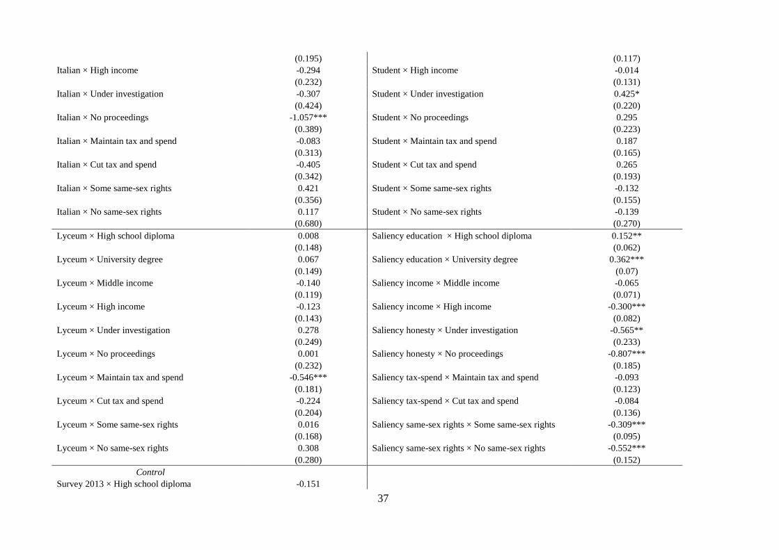
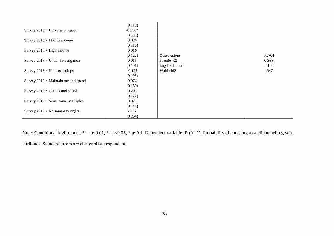
TABLE A. Voting, valence and policy attributes

Variables Estimate

(s.e.)

Variables Estimate

(s.e.)

Attributes of candidates Interactions between attributes

High school diploma 0.231

(0.552)

University degree 0.307 High school diploma × Maintain tax and spend 0.479***

(0.661) (0.128)

Middle income 0.581 High school diploma × Cut tax and spend 0.690***

(0.486) (0.221)

High income 0.793 University degree × Maintain tax and spend 0.087

(0.535) (0.113)

Under investigation 0.518 University degree × Cut tax and spend 0.023

(1.184) (0.124)

No proceedings 0.355 High school diploma × Some same-sex rights -0.470***

(1.153) (0.164)

Keep spend and tax levels 0.300 High school diploma × No same-sex rights -0.189

(0.787) (0.183)

Cut taxes and spending -0.840 University degree × Some same-sex rights -0.151

(0.946) (0.173)

Some rights to same sex couples -1.501** University degree × No same-sex rights -0.731***

(0.634) (0.261)

No rights to same sex couples -3.302***

(1.028)

Socio-demographic and political traits

Interest in politics × High school diploma 0.035 Ideology × High school diploma -0.039

(0.092) (0.026)

Interest in politics × University degree -0.02 Ideology × University degree -0.063**

(0.097) (0.03)

Interest in politics × Middle income 0.049 Ideology × Middle income -0.029

(0.08) (0.025)

Interest in politics × High income -0.009 Ideology × High income 0.038

(0.104) (0.029)

36

Interest in politics × Under investigation -0.202 Ideology × Under investigation 0.132***

(0.138) (0.043)

Interest in politics × No proceedings -0.346** Ideology × No proceedings 0.326***

(0.143) (0.043)

Interest in politics × Maintain tax and spend -0.078 Ideology × Maintain tax and spend 0.136***

(0.109) (0.033)

Interest in politics × Cut tax and spend -0.269** Ideology × Cut tax and spend 0.269***

(0.118) (0.040)

Interest in politics × Some same-sex rights 0.172 Ideology × Some same-sex rights 0.205***

(0.107) (0.029)

Interest in politics × No same-sex rights 0.088 Ideology × No same-sex rights 0.515***

(0.172) (0.048)

Male × High school diploma -0.179 Age × High school diploma -0.017*

(0.133) (0.01)

Male × University degree -0.043 Age × University degree -0.011

(0.140) (0.011)

Male × Middle income 0.023 Age × Middle income -0.011

(0.119) (0.014)

Male × High income 0.087 Age × High income -0.005

(0.135) (0.011)

Male × Under investigation 0.426** Age × Under investigation 0.014

(0.212) (0.017)

Male × No proceedings 0.391* Age × No proceedings 0.023

(0.202) (0.027)

Male × Maintain tax and spend -0.305* Age × Maintain tax and spend 0.01

(0.157) (0.017)

Male × Cut tax and spend 0.098 Age × Cut tax and spend 0.009

(0.177) (0.021)

Male × Some same-sex rights 0.339** Age × Some same-sex rights 0.018

(0.151) (0.014)

Male × No same-sex rights 0.975*** Age × No same-sex rights 0.015

(0.278) (0.022)

Italian × High school diploma -0.105 Student × High school diploma 0.026

(0.281) (0.123)

Italian × University degree -0.163 Student × University degree 0.198

(0.387) (0.132)

Italian × Middle income 0.023 Student × Middle income 0.151

37

(0.195) (0.117)

Italian × High income -0.294 Student × High income -0.014

(0.232) (0.131)

Italian × Under investigation -0.307 Student × Under investigation 0.425*

(0.424) (0.220)

Italian × No proceedings -1.057*** Student × No proceedings 0.295

(0.389) (0.223)

Italian × Maintain tax and spend -0.083 Student × Maintain tax and spend 0.187

(0.313) (0.165)

Italian × Cut tax and spend -0.405 Student × Cut tax and spend 0.265

(0.342) (0.193)

Italian × Some same-sex rights 0.421 Student × Some same-sex rights -0.132

(0.356) (0.155)

Italian × No same-sex rights 0.117 Student × No same-sex rights -0.139

(0.680) (0.270)

Lyceum × High school diploma 0.008 Saliency education × High school diploma 0.152**

(0.148) (0.062)

Lyceum × University degree 0.067 Saliency education × University degree 0.362***

(0.149) (0.07)

Lyceum × Middle income -0.140 Saliency income × Middle income -0.065

(0.119) (0.071)

Lyceum × High income -0.123 Saliency income × High income -0.300***

(0.143) (0.082)

Lyceum × Under investigation 0.278 Saliency honesty × Under investigation -0.565**

(0.249) (0.233)

Lyceum × No proceedings 0.001 Saliency honesty × No proceedings -0.807***

(0.232) (0.185)

Lyceum × Maintain tax and spend -0.546*** Saliency tax-spend × Maintain tax and spend -0.093

(0.181) (0.123)

Lyceum × Cut tax and spend -0.224 Saliency tax-spend × Cut tax and spend -0.084

(0.204) (0.136)

Lyceum × Some same-sex rights 0.016 Saliency same-sex rights × Some same-sex rights -0.309***

(0.168) (0.095)

Lyceum × No same-sex rights 0.308 Saliency same-sex rights × No same-sex rights -0.552***

(0.280) (0.152)

Control

Survey 2013 × High school diploma -0.151

38

(0.119)

Survey 2013 × University degree -0.228*

(0.132)

Survey 2013 × Middle income 0.026

(0.110)

Survey 2013 × High income 0.016

(0.122) Observations 18,704

Survey 2013 × Under investigation 0.015 Pseudo-R2 0.368

(0.196) Log-likelihood -4100

Survey 2013 × No proceedings -0.122 Wald chi2 1647

(0.198)

Survey 2013 × Maintain tax and spend 0.076

(0.150)

Survey 2013 × Cut tax and spend 0.203

(0.172)

Survey 2013 × Some same-sex rights 0.027

(0.144)

Survey 2013 × No same-sex rights -0.02

(0.254)

Note: Conditional logit model. *** p<0.01, ** p<0.05, * p<0.1. Dependent variable: Pr(Y=1). Probability of choosing a candidate with given

attributes. Standard errors are clustered by respondent.

Documents

Voting in a Multi-dimensional Space: a Conjoint Analysis