(VWLPDWLRQ - DiVA portal

INDEGREE PROJECT MECHANICAL ENGINEERING,SECOND CYCLE, 30 CREDITS

,

GPS-oscillation-robustLocalization and Vision-aided Odometry Estimation

HONGYI CHEN

KTH ROYAL INSTITUTE OF TECHNOLOGYSCHOOL OF INDUSTRIAL ENGINEERING AND MANAGEMENT

1

Examensarbete TRITA-ITM-EX 2019:10

GPS-oscillation-robust lokalisering och visionsstödd odometri uppskattning

Hongyi Chen

Godkänt

2019-02-03

Examinator

Lei Feng

Handledare

Xinhai Zhang CO: Milan Horemuz

Uppdragsgivare

Integrated Transport Research Lab

Kontaktperson

Yuchao Li

Sammanfattning GPS/IMU integrerade system används ofta för navigering av fordon. Algoritmen för detta

kopplade system är normalt baserat på ett Kalmanfilter. Ett problem med systemet är att oscillerade

GPS mätningar i stadsmiljöer enkelt kan leda till en lokaliseringsdivergens. Dessutom kan

riktningsuppskattningen vara känslig för magnetiska störningar om den är beroende av en IMU

med integrerad magnetometer.

Rapporten försöker lösa lokaliseringsproblemet som skapas av GPS-oscillationer och avbrott med

hjälp av ett adaptivt förlängt Kalmanfilter (AEKF). När det gäller riktningsuppskattningen används

stereovisuell odometri (VO) för att försvaga effekten av magnetiska störningar genom

sensorfusion. En Visionsstödd AEKF-baserad algoritm testas i fall med både goda GPS

omständigheter och med oscillationer i GPS mätningar med magnetiska störningar. Under de

fallen som är aktuella är algoritmen verifierad för att överträffa det konventionella utökade

Kalmanfilteret (CEKF) och ”Unscented Kalman filter” (UKF) när det kommer till

positionsuppskattning med 53,74% respektive 40,09% samt minska fel i riktningsuppskattningen.

Nyckelord: Adaptivt förlängt Kalmanfilter, lokalisering, stereovisuell odometri, GPS avbrott.

2

3

Master of Science Thesis TRITA-ITM-EX 2019:10

GPS-oscillation-robust Localization and Vision-aided Odometry Estimation

Hongyi Chen

Approved

2019-02-03

Examiner

Lei Feng

Supervisor

Xinhai Zhang CO: Milan Horemuz

Commissioner

Integrated Transport Research Lab

Contact person

Yuchao Li

Abstract GPS/IMU integrated systems are commonly used for vehicle navigation. The algorithm for this

coupled system is normally based on Kalman filter. However, oscillated GPS measurements in the

urban environment can lead to localization divergence easily. Moreover, heading estimation may

be sensitive to magnetic interference if it relies on IMU with integrated magnetometer.

This report tries to solve the localization problem on GPS oscillation and outage, based on adaptive

extended Kalman filter(AEKF). In terms of the heading estimation, stereo visual odometry(VO)

is fused to overcome the effect by magnetic disturbance. Vision-aided AEKF based algorithm is

tested in the cases of both good GPS condition and GPS oscillation with magnetic interference.

Under the situations considered, the algorithm is verified to outperform conventional extended

Kalman filter(CEKF) and unscented Kalman filter(UKF) in position estimation by 53.74% and

40.09% respectively, and decrease the drifting of heading estimation.

Key word: Adaptive Extended Kalman Filter, Localization, Stereo visual odometry, GPS

outage

4

Acknowledgements

Firstly I would like to thank my supervisor Xinhai Zhang to help me along thethesis work and review my thesis report.

Moreover, I really enjoyed working in Integrated Transport Research Lab to-gether with many talented people. Especially, I appreciate the research assistantJiajun Shi. With his kind help, I can hand on the hardware and software platformof RCV more easily. I also want to thank Mikael Hellgren to help solve the hardwareproblems when RCV stops working.

Additionally, I would appreciate my co-supervisor Milan Horemuz to give mesome suggestions and help verify my results.

Finally, I would express my sincere gratitude to my family and friends. Thanksto their supports, I can overcome the trouble and complete the thesis work.

5

Contents

1 Introduction 1

2 Background 32.1 Research Concept Vehicle . . . . . . . . . . . . . . . . . . . . . . . . 32.2 Sensors Introduction . . . . . . . . . . . . . . . . . . . . . . . . . . . 42.3 State Estimation Techniques . . . . . . . . . . . . . . . . . . . . . . 82.4 Estimation Problems in GPS/IMU Navigation System . . . . . . . . 11

3 Research Design and the State of the Art 153.1 Research Questions . . . . . . . . . . . . . . . . . . . . . . . . . . . . 153.2 Research Method . . . . . . . . . . . . . . . . . . . . . . . . . . . . . 163.3 Limitations . . . . . . . . . . . . . . . . . . . . . . . . . . . . . . . . 183.4 Related Work/State of Art . . . . . . . . . . . . . . . . . . . . . . . 18

4 INS/GPS Localization Based on AEKF 214.1 Vehicle Modeling . . . . . . . . . . . . . . . . . . . . . . . . . . . . . 21

4.1.1 Single-track Model . . . . . . . . . . . . . . . . . . . . . . . . 214.1.2 Double-track Model . . . . . . . . . . . . . . . . . . . . . . . 22

4.2 Coordinate System . . . . . . . . . . . . . . . . . . . . . . . . . . . . 244.3 Adaptive Extended Kalman Filter Algorithm . . . . . . . . . . . . . 254.4 Implementation . . . . . . . . . . . . . . . . . . . . . . . . . . . . . . 26

4.4.1 Hardware Analysis . . . . . . . . . . . . . . . . . . . . . . . . 264.4.2 Sensor Placement . . . . . . . . . . . . . . . . . . . . . . . . . 294.4.3 Software Platform . . . . . . . . . . . . . . . . . . . . . . . . 304.4.4 Coordinate Transform . . . . . . . . . . . . . . . . . . . . . . 314.4.5 Filter parameters & settings . . . . . . . . . . . . . . . . . . . 34

4.5 Experiment Results . . . . . . . . . . . . . . . . . . . . . . . . . . . . 364.5.1 Algorithm Performance on Good GPS Condition . . . . . . . 364.5.2 Localization on GPS Oscillation . . . . . . . . . . . . . . . . 40

4.6 Discussion . . . . . . . . . . . . . . . . . . . . . . . . . . . . . . . . . 44

5 Vision-aided Heading Estimation 475.1 Algorithm Introduction . . . . . . . . . . . . . . . . . . . . . . . . . 475.2 Yaw Rate Test . . . . . . . . . . . . . . . . . . . . . . . . . . . . . . 48

6

CONTENTS 7

5.3 Results and Discussion . . . . . . . . . . . . . . . . . . . . . . . . . . 49

6 Conclusion and Future Work 516.1 Conclusion . . . . . . . . . . . . . . . . . . . . . . . . . . . . . . . . 516.2 Future Work . . . . . . . . . . . . . . . . . . . . . . . . . . . . . . . 52

6.2.1 More Robust Sensor Assembly . . . . . . . . . . . . . . . . . 526.2.2 More Extensive Parameter Tuning . . . . . . . . . . . . . . . 526.2.3 Dynamic Vehicle Model . . . . . . . . . . . . . . . . . . . . . 526.2.4 Implementation of dual GPS system . . . . . . . . . . . . . . 52

Bibliography 53

8 CONTENTS

AbbreviationsAEKF Adaptive Extended Kalman Filter

AHS Active Heading Stabilization

CEKF Conventional Extended Kalman Filter

DOP Dilution of Precision

EKF Extended Kalman Filter

GNSS Global Navigation Satellite Systems

GPS Global Position System

IAE Innovation-based Adaptive Estimation

ICC In-run Compass Calibration

IMU Inertial Measurement Unit

ISPKF Iterated Sigma Point Kalman Filter

MFM Magnetic Field Mapper

ML Maximum Likelihood

NMS Non-maximum Suppression

PF Particle Filter

RANSAC Random Sample Consensus

RCV Research Concept Vehicle

RMSE Root Mean Square Error

ROS Robot Operating System

RPF Regularized Particle Filter

RTK Real Time Kinematic

SIRF Sampling Importance Resampling Filter

SLAM Simultaneous localization and mapping

UKF Unscented Kalman Filter

UT Unscented Transform

VO Visual Odometry

WO Wheel Odometry

List of Figures

2.1 KTH RCV (Research Concept Vehicle) . . . . . . . . . . . . . . . . . . 32.2 Positioning from IMU Measurements [5] . . . . . . . . . . . . . . . . . . 42.3 Xsens MTi-G-700 . . . . . . . . . . . . . . . . . . . . . . . . . . . . . . . 52.4 GPS Positioning in the Urban Environment[10] . . . . . . . . . . . . . . 52.5 Good and Poor Satellite Geometry [11] . . . . . . . . . . . . . . . . . . 62.6 Trimble SPS852 Modular GPS Receiver . . . . . . . . . . . . . . . . . . 62.7 Reach RTK Receiver . . . . . . . . . . . . . . . . . . . . . . . . . . . . . 62.8 RTK Positioning Principal[12] . . . . . . . . . . . . . . . . . . . . . . . . 72.9 ZED camera . . . . . . . . . . . . . . . . . . . . . . . . . . . . . . . . . 82.10 VBOX 3i Dual Antenna . . . . . . . . . . . . . . . . . . . . . . . . . . . 82.11 State Transition Graph . . . . . . . . . . . . . . . . . . . . . . . . . . . 92.12 EKF vs UKF [15] . . . . . . . . . . . . . . . . . . . . . . . . . . . . . . . 112.13 GPS/IMS Navigation Structure . . . . . . . . . . . . . . . . . . . . . . . 122.14 Linearization on the Sate with Different Uncertainties . . . . . . . . . . 12

4.1 Kinematic Bicycle Model . . . . . . . . . . . . . . . . . . . . . . . . . . 224.2 Kinematic Double-track Model . . . . . . . . . . . . . . . . . . . . . . . 234.3 ECEF and ENU Coordinate . . . . . . . . . . . . . . . . . . . . . . . . . 254.4 AEKF Algorithm Structure [16] . . . . . . . . . . . . . . . . . . . . . . . 254.5 MFM successful result [31] . . . . . . . . . . . . . . . . . . . . . . . . . 274.6 Yaw Rate calculated from steering encoders . . . . . . . . . . . . . . . . 284.7 Sensor Placement on RCV . . . . . . . . . . . . . . . . . . . . . . . . . . 294.8 Data Communication in RCV . . . . . . . . . . . . . . . . . . . . . . . . 304.9 Rqt Frame Tree . . . . . . . . . . . . . . . . . . . . . . . . . . . . . . . . 314.10 GPS coordinate Transform . . . . . . . . . . . . . . . . . . . . . . . . . 324.11 Testing Track . . . . . . . . . . . . . . . . . . . . . . . . . . . . . . . . . 364.12 Yaw Estimation by AEKF . . . . . . . . . . . . . . . . . . . . . . . . . . 374.13 Estimation at Low Speed . . . . . . . . . . . . . . . . . . . . . . . . . . 384.14 Estimation at High Speed . . . . . . . . . . . . . . . . . . . . . . . . . . 384.15 Position Estimation by AEKF . . . . . . . . . . . . . . . . . . . . . . . 394.16 Yaw Rate Estimation by AEKF . . . . . . . . . . . . . . . . . . . . . . . 404.17 GPS Signal on the Test Road . . . . . . . . . . . . . . . . . . . . . . . . 414.18 Position estimation by EKF . . . . . . . . . . . . . . . . . . . . . . . . . 424.19 Position estimation by UKF . . . . . . . . . . . . . . . . . . . . . . . . . 42

9

10 List of Figures

4.20 Position Estimation by AEKF (initial σ2 = 0.25) . . . . . . . . . . . . . 434.21 Position Estimation by AEKF . . . . . . . . . . . . . . . . . . . . . . . 434.22 Covariance Estimation by EKF . . . . . . . . . . . . . . . . . . . . . . . 454.23 Path Estimation by AEKF . . . . . . . . . . . . . . . . . . . . . . . . . 46

5.1 Yaw Rate Test between VO and WO . . . . . . . . . . . . . . . . . . . . 495.2 Yaw Estimation by AEKF with Vision Aided . . . . . . . . . . . . . . . 50

List of Tables

2.1 Comparison between VO and V-SLAM . . . . . . . . . . . . . . . . . . . 82.2 GPS Measurement Methods . . . . . . . . . . . . . . . . . . . . . . . . . 13

3.1 AEKF Algorithm Test on Good GPS condition . . . . . . . . . . . . . . 173.2 AEKF Algorithm Test on GPS oscillation . . . . . . . . . . . . . . . . . 173.3 Vision-aided Heading Estimation Test . . . . . . . . . . . . . . . . . . . 18

4.1 Message frequency . . . . . . . . . . . . . . . . . . . . . . . . . . . . . . 344.2 Observation Input . . . . . . . . . . . . . . . . . . . . . . . . . . . . . . 354.3 Yaw Estimation Error . . . . . . . . . . . . . . . . . . . . . . . . . . . . 374.4 Estimation Error at Low Speed . . . . . . . . . . . . . . . . . . . . . . . 384.5 Estimation Error at High Speed . . . . . . . . . . . . . . . . . . . . . . 384.6 Position Estimation Error (AEKF, EKF, and UKF) . . . . . . . . . . . 44

5.1 Yaw Rate Estimation Error between VO and WO . . . . . . . . . . . . 485.2 Vision-aided Heading Estimation . . . . . . . . . . . . . . . . . . . . . . 50

11

Chapter 1

Introduction

Autonomous driving is becoming a popular topic and its development grows rapidlywith abundant contributions from industry and research organizations. The au-tomation level can be divided into five stages, ranging from Driver Assistance (level1) up to full automation (level 5) [1]. Currently, a majority of vehicles still dependon drivers’ manual operations but possibly assisted by some safety systems to avoidpotential accidents. For instance, automatic braking system could help prevent thecollision with the pedestrian or other road users in front. Even more advanced inreality, on-road level 2 driving has already been possible due to ADAS(AdvancedDriver Assistance Systems), such as steering and lane control assistance, remoteparking systems, etc. The full automation remains under conceptual research sofar, however, highly and fully unmanned driving are developed rapidly due to thetechnique revolution in various areas, such as the great progress in machine learningand artificial intelligence. Without human inference, the perception of surround-ing environment relies on multiple sensors’ detection, such as IMU, GPS, Lidar orcamera on the vehicle. For instance, Tesla Model 3 uses eight cameras, a forwardradar and twelve ultrasonic sensors for its autopilot/auto-steering features [2]. Thecamera is responsible for auto-steering, in particular keeping the car in the lane,as well as detecting the surrounding environment such as pedestrian, obstacles andtraffic sign. While the radar is primarily used to determine relative speed to theobjects in front to achieve "Traffic Aware Cruise Control".

Redundant sensor inputs are fused to estimate more accurate vehicle states,which is of great importance for path planning and vehicle navigation control. Asfor the localization issue in automotive industry, GPS/IMU coupled fusion is nor-mally adopted and works effectively in the case where GPS reliably measures theposition. Moreover, during recent years, camera, lidar or radar are gradually utilizedto improve the robustness especially when GPS or IMU works improperly.

The thesis is proposed to develop an algorithm to localize the position and esti-mate the odometry for an electric vehicle with multiple sensors supported, includingwheel encoders, IMU, GPS, and stereo camera. The algorithm aims to overcome thelocalization problem on bad GPS condition, and heading estimation problem under

1

CHAPTER 1. INTRODUCTION

magnetic interference. The implementation platform is based on the RCV (Re-search Concept Vehicle), a battery electric vehicle made by KTH. The robustnessfor the estimator is concentrated to be researched on, especially its robustness topoor GPS measurements and magnetic interference. In Chapter 2, sensors and somecommon navigation techniques are basically introduced. Then, Chapter 3 clarifiesthe research questions and methods. The algorithm and implementation work arediscussed about in Chapter 4 and 5. Eventually, the conclusions derived from thethesis project and suggestions for the future work are summarized in Chapter 6.

2

Chapter 2

Background

2.1 Research Concept Vehicle

Research Concept Vehicle is a vehicle prototyping made by KTH for research, con-cept demonstration and verification. The RCV is shown in Figure 2.1 below.

Figure 2.1: KTH RCV (Research Concept Vehicle)

RCV is a steer-by-wire and drive-by-wire electric vehicle with different sensorsattached, to be more specific, two Velodyne lidars, one front ZED camera, encoders,Trimble GPS, Reach RTK GPS, and Xsens IMU. The communication network inRCV is divided into a lower and upper layer, which are based on CAN and Ethernetnetwork respectively. The network on the lower layer is principally responsible forthe interactions among dSpace autobox, actuator drivers, encoders, and XsenseIMU. While the Ethernet on the upper layer enables the connection from lidars,camera, GPS receiver to a ROS computer. The mutual data transmission betweenthis hierarchical network is bridged through UDP communication protocol. Moredescriptions of the networks and function assignments in RCV will be discussedabout in Chapter 4.

3

CHAPTER 2. BACKGROUND

In terms of basic dynamical properties for RCV, the maximum steering angleis ± 25 ◦ actuated by linear actuators [3]. Each wheel is driven by its hub motorwith the install torque at 150 Nm and rated maximum speed of 520 rpm, which canspeed the vehicle up to 55 km/h [4].

2.2 Sensors Introduction

Inertial Measurement Unit(IMU) is a self-contained electronic device that mea-sures linear and angular motion. Commonly, IMU consists of a triad of gyroscopesand accelerometers, but some types have magnetometers equipped. A 3-axis ac-celerometer measures the acceleration along x, y, z axes of IMU respectively, whilea 3-axis gyrosope measures angular velocity. In addition, a magnetometer is able tomeasure the earth magnetic field intensity and derive the global roll, pitch and yaw.Unfortunately, since RCV is an electric vehicle, it can generate strong electromag-netic field to distort the measurement of a magnetometer. However, it is possibleto derive the position by the angular velocity and acceleration from IMU, which isshown in Figure 2.2.

Figure 2.2: Positioning from IMU Measurements [5]

Deciphered from the figure above, the position is calculated from double inte-gration of accelerations after the subtraction by gravitational acceleration g, whichcan accumulate the error from a gyro bias. Moreover, when RCV is driven uphillor downhill, the vertical acceleration is no more aligned with the gravity direction,which also leads to inaccurate positions.

In RCV, Xsens MTi-G-700 with GNSS(Global Navigation Satellite Systems)aided is adopted for use, which is shown in Figure 2.3. It can provide precise mea-surements with 10 deg/h gyro bias stability and 0.8 deg yaw measurement accuracy.In order to improve the yaw measurement, there are two calibration algorithms inthis type of Xsens IMU, that are AHS(Active Heading Stabilization) [6] and ICC(In-run Compass Calibration) [7]. AHS is aimed at tackling the magnetic distortionsthat do not move with the sensor, such as temporary or spatial distortions in thesurrounding environment. Some other distortions such as calibration errors, impactfrom the materials of hard and soft iron cannot be removed by AHS effectively.Fortunately, those distortions can be estimated by MFM(Magnetic Field Mapper)

4

2.2. SENSORS INTRODUCTION

[8] calibration. Instead of being north-referenced, the yaw output will be referencedwith respect to startup heading after AHS is enabled. According to the specializa-tion of MTi series in the product documentation, with AHS assisted, the driftingerror of the yaw measurement can be reduced by 1 deg for the MTi 100-series and 3deg for the MTi 10-series after 60 min [6]. Furthermore, imperfect MFM calibrationand inhomogenous magnetism can also introduce some errors.

Figure 2.3: Xsens MTi-G-700

Global Position System(GPS) is a satellite-based radio-navigation systemthat provides the geolocation and time information of anywhere on the Earth wherethere are unobstructed lines of sight to at least 4 satellites [9]. GPS works by con-necting the receiver to multiple satellites around the space and localize the positiongiven radio speed, locations of satellites, and the time for signal travelling. In termsof GPS/IMU navigation problem, IMU works well at measuring accelerations andyaw rate, but diverges the position due to the error accumulated from gyro bias.Fortunately, this divergence can be corrected by the GPS global positioning.

However, GPS signal can oscillate from time to time due to some environmentalfactors, such as atmosphere refraction and dense urban regions. Figure 2.4 showsthe GPS oscillation when the vehicle is driven at the dense district where crowdedbuildings stand aside.

Figure 2.4: GPS Positioning in the Urban Environment[10]

In addition, bad satellite geometry also degrades the precision, which can beexpressed by DOP(Dilution of Precision) [11]. DOP can be classified into “math-ematical” and “geometrical” DOP. The latter one is equal to the reciprocal of the

5


volume of a tetrahedron shaped by satellites. Generally, if a DOP becomes larger,the worse GPS signal is received, and vice versa. For example, in Figure 2.5, thevolume of tetrahedron on the left picture is obviously greater than the right one,which corresponds to a smaller DOP and better GPS measurement. In the worstcase, a infinite value of DOP can be derived when satellites are aligned in a straightline. Therefore, even though many satellites are available to be detected, there stillexists a possibility of GPS outage due to poor satellite geometry.

Figure 2.5: Good and Poor Satellite Geometry [11]

Trimble SPS852 Modular GPS receiver is equipped on RCV originally. WithRTK(Real Time Kinematic) service facilitated, Trimble GPS is able to localize thevehicle in centimeter-level accuracy. Unfortunately, Trimble was no longer able tobe set up due to limited knowledge on RCV network and undesirable change on theconfiguration by previous users. Therefore, it was replaced by Reach RTK(shownin Figure 2.7) during some tests. However, Trimble GPS without RTK setup stillcan provide accurate position in an open environment with good satellite geometry.

Figure 2.6: Trimble SPS852 Modular GPS Receiver

Figure 2.7: Reach RTK Receiver

6

2.2. SENSORS INTRODUCTION

The working principal of RTK is demonstrated in Figure 2.8. RTK techniqueestablishes the network amongst GNSS satellite, rover station, and base station. Abase station is particularly responsible for post-processing the data received fromsatellites and transmitting to a rover station. A rover station receives the carrierwave, meanwhile corrects the position using the signal from a base station. WithRTK technique assisted, it becomes possible to localize the vehicle in the accuracyup to 1 cm + 1 ppm under good GPS condition.

Figure 2.8: RTK Positioning Principal[12]

Wheel Odometry(WO) calculates the vehicular state only by a vehicle’s kine-matics and speed. The incremental encoder and absolute encoder are commonlyused to measure rotational velocity and position. RCV has four incremental en-coders attached to the wheel axle to measure the velocity of front wheels and rearwheels respectively. Apart from that, the other four encoders measure the steeringangle of each wheel. In contrast to absolute encoders, the incremental encoders inRCV cannot store the steering angle after power-off, which might introduce initialmeasurement errors when RCV is restarted.

Visual Odometry(VO) estimates the ego-motion of a stereo camera by asso-ciated images, which is widely used in autonomous driving in recent years. Visualodometry derived by stereo camera is named stereo VO. It estimates camera mo-tion by computing relative rotation and translation between 3D landmarks whichare triangulated from stereo-matched image features. Moreover, the stereo VOcan avoid scale ambiguity in monocular VO and work more efficiently than visualSLAM(Simultaneous localization and mapping). Table 2.1 compares differencesbetween VO and SLAM method.

7


Table 2.1: Comparison between VO and V-SLAM

Vision-based Technique Visual Odometry Visual SLAMProblem Focus Local trajectory Global trajectory, map

Optimization range Last poses of the path Loop closure, globallyComputational Cost Low HighEstimation Accuracy Low High

As is compared in the table, visual odometry has no dependency on prior knowl-edge of maps and has lower computational cost than visual SLAM. In the the-sis project, ZED stereo camera(shown in Figure 2.9) is utilized to generate visualodometry with 20 meters maximum detection range and up to 100Hz sampling fre-quency [13]. Moreover, the package of ZED camera provides a simple interface toROS(Robot Operating System).

Figure 2.9: ZED camera

VBOX 3i Dual Antenna is a high-quality industrial product made by VBOXAutomotive company, which is shown in Figure 2.10. It measures the acceleration,velocity and roll/pitch/yaw angle with twin antennas connected. According to thespecialization documented in VBOX website, it can measure the heading in 0.1◦accuracy with the resolution of 0.01◦, and the velocity in 0.1km/h accuracy [14].Thereby, VBOX is sufficient to provide the ground truth for algorithm tests.

Figure 2.10: VBOX 3i Dual Antenna

2.3 State Estimation TechniquesThe localization problem substantially is to estimate a dynamic state relying on ob-servations from various sensors. The estimation is simply based on Bayesian filter,

8

2.3. STATE ESTIMATION TECHNIQUES

which consists of prediction and update stage. Bayesian filter recursively estimatesthe state based on Markov model, which is indicated in Figure 2.11. In a Markovchain, the conditional probability of the present state xt only relies upon the latestprevious state xt−1, rather than on the sequence of preceded states. The transitionbetween states goes through the process/motion model interfered by the controlsignal ut, which is reflected on the prediction stage of Bayesian filter. Meanwhile,There exists a variety of measurements zt observed from the state xt to correct thepredicted state on the update stage. The equations in prediction and update stepare expressed as followed:

The Prediction Step:

p(xt | z1, ..., zt−1, u1, ..., ut)

=∫p(xt | xt−1, ut)p(xt−1 | z1, ..., zt−1, u1, ..., ut−1)dxt−1

(2.1)

The Correction Step:

p(xt | z1, ..., zt) ∝ p(xt | z1, ..., zt−1) (2.2)

Figure 2.11: State Transition Graph

Extended Kalman Filter(EKF) is a nonlinear version of conventional Kalmanfilter by linearizing an estimate of mean and covariance. In EKF, the motion andobservation model are no longer linear functions but expressed by differentiablefunctions instead, which are indicated by equations (2.3), (2.4).

9


System Description

xk = f(xk−1, uk) (2.3)zk = h(k − 1) (2.4)

Prediction:

xk = f(xk−1, uk) (2.5)Pk = APkAT + Q (2.6)

Update:

K = PkHT (HPkHT + R)−1 (2.7)xk+1 = xk + K(zk − h(xk)) (2.8)

Pk+1 = (I−KH)Pk (2.9)

Innovation:

dk = zk − h(xk) (2.10)

residual:

εk = zk − xk+1 (2.11)

As is shown in the above equations (2.3) - (2.4), both motion model f(x) andobservation model h(x) are nonlinear originally. In order to calculate the stateuncertainty, the motion model will be linearized at the mean point of the currentstate’s Gaussian distribution by Jacobian matrix on the prediction stage, which isdenoted as matrix A in the equations. Similarly, matrix H denotes the observationmodel linearized on the update stage. After that, Kalman gain K is used to balancethe weight between the predicted state and observations and derive the mean anduncertainty of the current state estimate.

UKF(Unscented Kalman Filter) is an estimation technique invented to solve lin-earization problems. UKF selects the weighted points in symmetric pairs(so called“sigma points”) from the Gaussian distribution of the original state and then propa-gates the points directly through the nonlinear model by UT(Unscented Transform).UT is a method to calculate the statistics of a random variable to approximate thenonlinear relationship [15]. Therefore, without linearization in UKF, the approxi-mation error can be reduced. Moreover, UKF is more advantageous to estimate thestate if the transformed state is not distributed as Gaussian, which is demonstratedin Figure 2.12. In the case where the actual state after transformation is no moredistributed as Gaussian, both mean and covariance of the state estimated by UKFare much closer to the ground truth than linearized EKF.

10

2.4. ESTIMATION PROBLEMS IN GPS/IMU NAVIGATION SYSTEM

Figure 2.12: EKF vs UKF [15]

AEKF(Adaptive Extended Kalman Filter) adaptively estimates the covariance ofprocess noise and measurement noise based on innovation (2.10) and residual (2.11)to improve the accuracy of state estimation with covariance varying[16]. In termsof CEKF(Conventional Extended Kalman Filter) , the covariance either of processnoise or measurement noise is fixed and unchanged during the estimation proce-dure. Therefore, estimation based on CEKF might lead to some problems whenthe covariance is not known in prior or varies during the estimation procedure. Forinstance, when Kalman filter is used to estimates the dynamic state of synchronousmachine in order to monitor and control the stability of its power system, wrongselection of the initial covariance matrices can diverge the estimate on rotor speedand angle easily. However, AEKF can be helpful to estimate the unknown covari-ance even though wrong covariances are initialized. Moreover, AEKF also functionsbetter in the case where measurement noise varies from time to time. A typical ap-plication is in GPS/IMU navigation system[17]. The phenomenon that GPS signaloscillates in the urban environment reflects the covariance change. Given a properGPS measurement covariance in real time, Kalma filter can estimate the positionin a more robust way.

2.4 Estimation Problems in GPS/IMU Navigation System

The common GPS/IMU navigation structure is demonstrated in Figure 2.13. Theestimator fuses the odometer, GPS and IMU together to estimate the vehicularstate. In Kalman filter based estimator, the predicted state is derived from thevehicle’s motion model and corrected by odometer, GPS, IMU observations sequen-tially on the update stage.

11


Figure 2.13: GPS/IMS Navigation Structure

The estimation challenges of the vehicle navigation problem mainly includes thesetwo topics: the linearization problem, and GPS oscillation and outage.

1. As is discussed in the previous section, EKF is commonly used in the vehiclelocalization due to its simplicity for practice and robustness. During the predictionstep in EKF, if the motion model is nonlinear, the linearization on the model canintroduce the approximation error, such as when a vehicle steers. This error can beimpacted by the covariance/uncertainty of the state, which is indicated in Figure2.14.

Figure 2.14: Linearization on the Sate with Different Uncertainties

Figure 2.14 shows the result when the state of different covariances is linearized.The Guassian distribution on the bottom represents the uncertainty of the initialstate or the state updated from previous estimate. The curve above it describesthe nonlinear transform function for the motion model. The diagram on the lefttop compares the distribution of the transformed state and ground truth, whichare expressed as the red and blue plot respectively. As can be observed, the meanof the predicted state approaches the actual mean more with the original stateuncertainty increasing. Therefore, it can be concluded that the linearization errorin EKF cannot be removed but can be reduced by increasing the state uncertainty.

On the other hand, high nonlinearity of a motion model also incurs great errors inEKF, such as when a vehicle is driven in a roundabout. Given identical distribution

12

2.4. ESTIMATION PROBLEMS IN GPS/IMU NAVIGATION SYSTEM

of the initial state, a transform function with higher nonlinearity leads to greaterapproximation errors.

2. The reliability of GPS measurement is mainly influenced by geometry ofsatellites, which corresponds to its covariance given to Kalman filter. The GPScovariance plays an important role in outlier detection and state estimation forKalman filter. When the GPS signal with a large DOP is received, the covarianceof GPS observation should be adjusted to be larger at the same time in order tobalance the predicted state on the update stage. However, a bad GPS measurementwith larger covariance can be more likely to be classified as an inlier by Mahalanobisthreshold [18] in Kalman filter, which is not expected in the case of GPS outage. Inaddition, different measurement methods and GPS receivers also constrain the GPSaccuracy, which is shown in Table 2.2. For example, with the receiver of C/A-codeand L1 frequency adopted, the GPS measured absolutely with 19 meters deviationcan still be considered as valid information for use, otherwise should be categorizedas an outlier.

Table 2.2: GPS Measurement Methods

Method Receiver ObservationTime

HorizontalUncer-

tainty(95%)[m]

Vertical Uncer-tainty(95%)[m]

Absolutely C/A-code,L1 1s 19 39

Absolutely P-code,L1& L2 1s 3 6

PPPAbsolutely Code phase,L1& L2 >1h 0.05 0.10

DGPSRelatively C/A-code,L1 1s 1 2

RTKRelatively Code phase,L1 & L2 1s 0.03 0.05

StaticRelatively Code phase,L1 & L2 >1h <0.01 <0.02

13

Chapter 3

Research Design and the State of the Art

RCV provides multiple sensors including a front stereo camera, Lidars, IMU, GPS,and encoders. It is possible to implement an advanced filter to overcome GPSoscillation by only fusing GPS, IMU, and encoders. Apart from the position esti-mate, heading is also very important information for advanced motion control inautonomous driving. However, the magnetic interference from RCV and the sur-rounding environment can affect the heading estimate. To overcome this headingerror, visual odometry could be an alternative.

3.1 Research Questions

GPS/IMU based Localization with conventional Kalman filter has problems of highdependency on the GPS position and IMU yaw. Especially within the urban en-vironment, undesirable GPS oscillation has a negative impact on position estimatedue to crowded buildings and bridges. Furthermore, GNSS satellite geometry withlarge DOP can also degrade the estimator performance on positioning. For pathplanning and following in autonomous vehicle, a consecutive positioning is of greatimportance to avoid undesirable control behaviour. GPS, as the only reliable mea-surement to correct the position in Kalman filter, fluctuates with varying covariance.Therefore, assuming the covariance of GPS signal can be estimated and applied toKalman filter in real time, the Kalman filter can work better at balancing weightsbetween the predicted state and measurements, which may result in a more con-secutive and accurate position estimate. Adpative extended Kalman filter, which isdifferent from EKF and UKF, adjusts the covariance of measurement and processnoise dynamically according to the sequence of previous state estimates. This mightimprove the localization performance under GPS oscillation.

Question 1: Through some experiments, can AEKF (Adaptive Extended KalmanFilter) outperform CEKF (Conventional Extended Kalman Filter) and UKF (Un-scented Kalman Filter) in terms of estimation accuracy, and robustness to GPSoscillation and outage?

IMU, usually consists of a gyroscope, accelerator and magnetometer. It pro-

15

CHAPTER 3. RESEARCH DESIGN AND THE STATE OF THE ART

vides measurements such as yaw, yaw rate and acceleration on longtitudinal andlateral directions. However, Since RCV is an electric-driven vehicle, the gener-ated magnetic field can distort the magnetometer in IMU, which can influence theyaw estimate indirectly. Fortunately, Xsens IMU has the algorithm - AHS(ActiveHeading Stabilization) to help measure the yaw angle under magnetic interference.However, even with AHS assistant and proper isolation, the yaw measured fromIMU still drifts due to calibration errors, magnetic interference from RCV and thesurrounding environment. Visual odometry, which is independent to the magneticfield, can be an alternative to compensate the error of yaw measurements.

Question 2: Can visual odometry improve the accuracy and constrain thedrifting error of heading estimate due to magnetic interference?

3.2 Research Method

The sensors utilized for algorithm design have never been tested, therefore sensoranalysis should be done in highest priority. During the tests, IMU should be cal-ibrated and configured to the AHS alogrithm setting, while the accuracy of GPSalso needs to be evaluated, including Trimble GPS, Xsens GPS and Reach RTKGPS. After the sensor test completed, it is essential to reattach sensors on properpositions on RCV, for instance, IMU should be fixed away from the RCV motors toreduce electromagnetic disturbance. With the hardware well-prepared, the softwarecan be designed.

The experiment should be divided into three different cases, which are listed asfollowed:

Experiment 1. AEKF Algorithm Test on Good GPS Condition. The purposeof this experiment is to verify if the AEKF algorithm can perform well in a goodGPS condition and improve the state estimation. The test track is selected inan open environment where not many buildings can block GPS signals. Duringthe experiment, the velocity, yaw and yaw rate are compared with the groundtruth provided by Vbox. Reach RTK GPS can provide centimeter-level positionmeasurements when the GPS receiver is in“Fix” status [19] under sufficient satellitesavailable. This perfect GPS is fused into the AEKF algorithm and used to providethe ground truth of position as well. If the path estimated by AEKF follows theGPS path, it can verify that AEKF localize the vehicle well on good GPS condition.The experiment design is summarized in table 3.1.

16

3.2. RESEARCH METHOD

Table 3.1: AEKF Algorithm Test on Good GPS condition

Experiment Design ContentTest Environment Open environment, cars parked aside the roadFused Sensors Xsens IMU, Reach RTK GPS, Wheel OdometryGround Truth Vbox, Reach RTK GPSTest Target Position, velocity, yaw, yaw rate

Evaluation Method RMSE (root mean square error)

Experiment 2. AEKF, CEKF, and UKF Test on GPS oscillation. To guaranteedifferent algorithms are tested under the same condition, sensor data is recorded toa ROS bag and replayed offline. The track is selected from google map in prior andincludes some regions with crowded buildings aside in order to test the algorithmon GPS oscillation. In the experiment, Reach RTK was replaced by Trimble GPSbecause Reach RTK GPS(with RTK set-up) can provide precise positions in “Fix”or “Float” status but can completely give unusable measurements under worse GPScondition due to its single-frequency receiver. However, even though Trimble GPS(without RTK set-up) has lower positioning accuracy but it still can provide goodpositions in decimeter-level under good satellite geometry, and gives oscillated butconsecutive position in dense areas. Therefore, since Reach RTK GPS is not beable to localize in the dense urban environment, GPS regression from Trimble GPSwas utilized for the ground truth in the experiment. In addition, RMSE(root meansquare error) was used to compare the localization accuracy amongst various algo-rithms. Apart from that, the sensitivity to GPS outliers and the smoothness of aestimated path can also be observed from the results. The experiment design issummarized in Table 3.2.

Table 3.2: AEKF Algorithm Test on GPS oscillation

Experiment Design ContentTest Environment Crowded buildings on both sides of the roadFused Sensors Xsens IMU, Trimble GPS, wheel odometryGround Truth GPS regressionTest Target Position

Evaluation Method RMSE, robustness to GPS outliers, path smoothness

Experiment 3. Heading Estimate Test under Magnetic Interference. In order toensure IMU is exposed to magnetic interference, the experiment was conducted onthe road where some other vehicles were parking aside, which can affect IMU byinterference from ferromagnetic materials. Because RCV is a battery electric car,it can generate inhomogenous magnetic field when steering and changing speed.Therefore, a tight turning is selected for the test track. The experiment design issummarized in Table 3.3.

17


Table 3.3: Vision-aided Heading Estimation Test

Experiment Design ContentTest Environment Open environment, cars parked aside the roadFused Sensors Xsens IMU, Reach RTK GPS, wheel odometry, visual odometryGround Truth VboxTest Target Yaw

Evaluation Method RMSE , drifting errors

The detailed experiments are discussed about in Chapter 4, 5 based on theresearch method design.

3.3 Limitations

In experiment 2, it is not possible to provide the ground truth in dense areas byReach RTK GPS because the noise due to signal multipath are amplified in a single-frequency receiver. Due to limited knowledge on RCV network and undesirablechange on the configuration by previous users, Trimble GPS cannot be setup withRTK service. However, it still can provide GPS measurements in decimeter-levelunder good GPS condition, and gives consecutive oscillated measurements in densestreets. During the experiment, RCV was driven along the road predetermined onGoogle map and straightforward on poor GPS regions on purpose. Therefore, theground truth can be regressed by these good Trimble GPS measurements, which issufficient for the comparison among AEKF, CEKF, and UKF.

It might be better to record the data and replay it offline to compare the headingestimate with and without visual odometry fused on the same dataset. However,the communication between a ZED camera and ROS could be broken down whenimage data are recorded into a ROS bag during the experiment 3. Instead, thevision-aided test was conducted right after the test case with no visual odometryfused in order to keep the same preconditions. Without visual odometry fused,yaw estimate highly depends on IMU yaw, therefore the drifting of IMU yaw cancause the error of yaw estimation. Therefore, if visual odometry can prevent theyaw estimate from drifting as IMU yaw and decrease RMSE, it can be sufficientto prove that visual odometry indeed can improve the heading estimation undermegnetic interference.

3.4 Related Work/State of Art

A great amount of researches contribute to the localization problem for unmannedvehicles. Conventionally, a Kalman filter based GPS/IMU coupled system is im-plemented on navigation. Rezaei, et al. applied extended Kalman filter to fuse thewheel odometer, yaw rate gyro and GPS measurement [20]. The experiment result

18

3.4. RELATED WORK/STATE OF ART

from Rezaei’s research indicated EKF can carry out the estimation on more than60 km distance even under slightly bad GPS condition. In order to cope with thelinearization problems in EKF, a bunch of new filters were put forwards. Rudolph,et al. developed a new filter framework, called Sigma-point Kalman filter, whichwas verified to outperform EKF in GPS/IMU navigation system under the samecomputational complexity [21]. It improved the position estimate by 30% than EKFthrough the experiment on an unmanned aerial vehicle. Jeong, et al. implementedSIRF(Sampling Importance Resampling Filter) and RPF(Regularized Particle Fil-ter), which are variants of PF(Particle Filter) [22], on the mobile robot localizationand proves that PF performs better than EKF in position and heading estimate.PF is an estimate technique using Monte Carlo algorithms for dynamic state es-timation, which does not require the prior assumption of a Gaussian distribution.Instead, a bunch of weighted particles are used to describe the state probability.This can reduce the linearization error but may have the problems of high compu-tational cost. St-Pierre, et al. compared the performance of UKF and EKF on anavigation system [23]. Principally, the UKF itself takes more advantages to dealwith the linearization errors than EKF, but it is not effective in the case where noGPS is available, which is shown in Mathieu’s tests. In addition, low dynamics ofthe vehicle can make the linearlization error in EKF negligible. Moreover, UKF hasa drawback of more computational time than EKF.

Since the vehicle localization relies on GPS to correct the predicted state, CEKFwith fixed covariances can diverge the position estimate on GPS oscillation andoutage. In order to deal with the noisy measurements in EKF, El-Sheimy, et al.proposed a fuzzy-augmented Kalman filter to compensate the error from measure-ment update [24]. The fuzzy model needs inputs extracted from the outputs of IMUmechanization equations and the errors of position and velocity to train the modelparameters. This method can effectively improve the estimation performance dur-ing GPS outage according to the research, but its complicated structure is hard forimplementation. Bistrovs, et al. evaluated the UKF, EKF on poor GPS occasions.The result came out that UKF could better tolerate unreliable GPS [25].

In stead of using the fixed covariances, another solution can be to estimate theGPS covariance dynamically. According to the introduction from section 2.2 men-tioned, a poor satellite geometry, corresponds to a small DOP, can scale up thepoor GPS measurements. Mathematically, DOP is equal to the square root sum ofthe main diagonal elements in a covariance matrix. Therefore, the GPS oscillationcan be reflected by the change on GPS covariance. Mohamed, et al. proposed aapproach - IAE(Innovation-based Adaptive Estimation) to estimate variable covari-ances in GPS/IMU navigation systems [26]. This scalar adaptive estimator is basedon the ML(Maximum Likelihood) and an innovation V-C matrix that is computedfrom a previous innovation sequence. However an innovation-based estimator can-not guarantee the measurement covariance derived to be positive. In order to dealwith this problem, a AEKF(Adaptive Extendd Kalman Filter) with a residual-basedestimation on the measurement covariance are utilized in the research of Wang [27]and Akhlaghi, et al. [16], which is also applied in this thesis project to overcome

19


unreliability problems of GPS. More details will be discussed in the following sec-tions.

Visual Odometry estimates frame-to-frame motion by image matching. Kitt,et al proposed an algorithm to estimate ego-motion based on a trifocal geometrybetween image triples [28]. They applied an ISPKF(Iterated Sigma Point KalmanFilter) combined with a RANSAC-based(Random Sample Consensus) outlier re-jection scheme to improve the robustness of VO(visual odometry). However, areal-time VO highly depends on high computational performance of a processingunit. This problem is improved by Geiger, et al., who proposed an more efficientvisual odometry with faster feature matching [29] than Kitt’s algorithm[28].

20

Chapter 4

INS/GPS Localization Based on AEKF

4.1 Vehicle Modeling

Vehicle modeling plays a crucial role in wheel odometry. Using speed and steeringangle measured by wheel encoders, wheel odometry can be calculated by the vehiclemodel. Methodology in dynamics modeling can be categorized into kinematic modeland dynamic model. In the thesis, only kinematic model is used for computing wheelodometry without considerations of a vehicle’s mass and yaw inertia, and tire model.Moreover, the modelling methods also can be classified into single-track model anddouble-track model. The former one, commonly used for vehicle modelling, hasless complexity to build dynamics relation. However, this might introduce greatermodelling errors in comparison to double-track model for RCV due to differentsteering dynamics.

In the filter, the wheel odometry provides the observations of longitude andlatitude velocity, yaw rate, and yaw for Kalman filter. Especially yaw rate andvelocities are highly concerned since the absolute yaw is accumulated from yaw ratebased on the previous heading estimate.

4.1.1 Single-track Model

Single-track model is also known as bicycle model. Its description is demonstratedin Figure 4.1. It can describe vehicle behaviours on various occasions with lesscomplexity. During modelling, two wheels on each axle can be replaced by one singlewheel for simplified calculation. The nonlinear equations describing this kinematicbicycle model are listed below [30], from equation (4.1) to (4.4):

21

CHAPTER 4. INS/GPS LOCALIZATION BASED ON AEKF

β = tan−1(( LrLf + Lr

)tan(αf )) (4.1)

ω = σ = vLr

sin(β) (4.2)

vx = x = v cos(β) (4.3)vy = y = v sin(β) (4.4)

Here, (X,Y) is an inertial frame while x and y coordinating the center of thevehicle. σ is the inertial heading and β is the angle between the velocity of thebody center, which is v indicated in Figure 4.1, and the longitudinal axis of thevehicle. As deciphered from the geometric relation in bicycle model, the heading(or the absolute yaw angle with respect to the (X,Y) coordinate) ω can be simplycalculated by (σ + β), in which β can be derived from the steering angle of a frontwheel αf . Then combined with current velocity v, the longitudinal and lateralvelocity can be obtained. Note that Lf and Lr are the distances from a front wheeland rear wheel to the center of the car respectively.

Figure 4.1: Kinematic Bicycle Model

4.1.2 Double-track ModelRCV has high performance on steering mainly due to its capability to turn rearwheels freely. This special design optimizes the steering system with higher curva-tures but increases the complexity of the vehicle dynamics. Double-track model can

22

4.1. VEHICLE MODELING

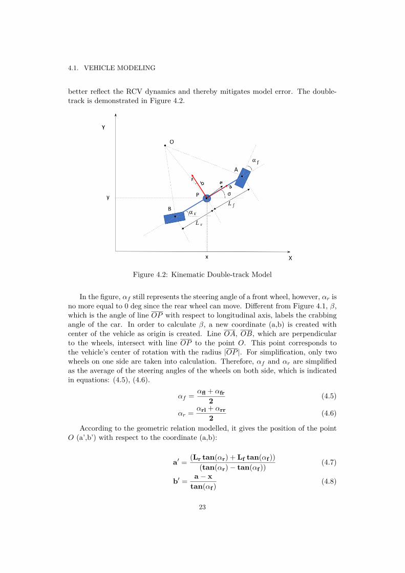
better reflect the RCV dynamics and thereby mitigates model error. The double-track is demonstrated in Figure 4.2.

Figure 4.2: Kinematic Double-track Model

In the figure, αf still represents the steering angle of a front wheel, however, αr isno more equal to 0 deg since the rear wheel can move. Different from Figure 4.1, β,which is the angle of line OP with respect to longitudinal axis, labels the crabbingangle of the car. In order to calculate β, a new coordinate (a,b) is created withcenter of the vehicle as origin is created. Line OA, OB, which are perpendicularto the wheels, intersect with line OP to the point O. This point corresponds tothe vehicle’s center of rotation with the radius |OP |. For simplification, only twowheels on one side are taken into calculation. Therefore, αf and αr are simplifiedas the average of the steering angles of the wheels on both side, which is indicatedin equations: (4.5), (4.6).

αf = αfl + αfr2 (4.5)

αr = αrl + αrr2 (4.6)

According to the geometric relation modelled, it gives the position of the pointO (a’,b’) with respect to the coordinate (a,b):

a′ = (Lr tan(αr) + Lf tan(αf ))(tan(αr)− tan(αf ))

(4.7)

b′ = a − xtan(αf )

(4.8)

23


Then, with the position of the point O (a’,b’) determined, the radius R ordistance from the axis of rotation can be calculated as below:

R = |OP| =√

a′2 + b′2 (4.9)

Eventually, the crabbing angle can be computed in equations below:

β =

−|tan−1(a

′

b′)| , if a′ · b′ > 0

|tan−1(a′

b′)|, , if a′ · b′ < 0

(4.10)

Meanwhile, calculate the yaw omega, longitudinal and lateral velocity ω, vx, vy:

ω = v cos(β)R (4.11)

vx = v cos(β) (4.12)vy = v sin(β) (4.13)

Note that heading ω is integrated by yaw rate based on the previous headingestimate to decrease error accumulation.

4.2 Coordinate SystemIn terms of GPS positioning used in vehicle navigation, the transformation fromglobal to local position coordinates involves five different coordinate systems: thegeodetic coordinate system, the (UTM) coordinate system, the (ECEF) coordinatesystem, the local (ENU) coordinate system, and the body-fixed coordinate system.The geodetic system is a reference system for describing a points in latitude andlongitude globally[32]. Similarly, the universal transverse mercator (UTM) coordi-nate system uses map projection by secant transverse Mercator with 2-dimensionalCartesian coordinate system to give locations on the surface of the Earth [33].The relation between ECEF and local ENU system can be described in figure 4.3.ECEF, a coordinate system with the origin defined as the center of mass of Earth,can be transformed from geodetic coordinates, which is similar to the conversion toUTM[34]. The local frame, normally referenced by east-north-up, provides referencefor the local position converted from ENU or UTM coordinate and places its originat the starting point of the vehicle movement. The body-fixed coordinate, locatedin the same spatial space as local ENU coordinate, takes the center of the mass ofthe car as an origin and aligns x,y axis to the directions of longitudinal and lateralvelocity respectively.

Both Trimble and Reach GPS can provide position information in UTM format.The location of the vehicle in local frame can be converted from UTM earth framethrough translation and rotation between coordinate systems. More details will bediscussed in the next section.

24

4.3. ADAPTIVE EXTENDED KALMAN FILTER ALGORITHM

Figure 4.3: ECEF and ENU Coordinate

4.3 Adaptive Extended Kalman Filter AlgorithmThere are multiple adaptive Kalman filter algorithms researched for dynamic stateestimation. In terms of the AEKF algorithm used in this thesis project, the measure-ment covariance is estimated based on residual, while the process noise covarianceis based on innovation. The detailed algorithm structure is demonstrated in Figure4.4.

Figure 4.4: AEKF Algorithm Structure [16]

AEKF can recursively update measurement covariance based on innovation us-

25


ing:

Rk = Sk −H[1]k P−k H[1]T

k (4.14)

Here Sk refers to the covariance matrix of the innovation. However, this equationcannot guarantee the estimated measurement covariance Rk be a positive matrixsince subtraction between Sk and HkPkH

Tk might lead to a negative result. There-

fore, in order to ensure the Rk is calculated to be a positive matrix, a residual-basedapproach proposed by[27] is used as:

εk = zk − hk(xk) (4.15)Sk = E[εεT] (4.16)

Rk = Sk + H[1]k P−k H[1]T

k (4.17)

Note that the expression εk is the residual. In equation (4.16), Sk calculated byaveraging εεT must be a positive matrix. Consequently, the result of equation 4.17is always positive. There are basically two methods to calculate the average valueof εεT . One is to use sliding window[35], while the other solution is to introduce aforgetting factor α[36], which helps save the memory and is simpler to implement.Then the equations can be transformed as below.

Rk = αRk−1 + (1− α)(εεT + HP−k H[1]Tk ) (4.18)

With a forgetting factor α (0<α<1) employed, preceding states becomes lessand less effective on current covariance estimation along the process. A larger α canincrease the weight on previous estimates, which prevents the covariance estimatefrom frequent oscillation but may incur longer time delays to catch up with changes.In the paper [16], α = 0.3 is used for the studies.

The process noise Q is estimated based on innovation in the AEKF algorithm.Similarly, using a forgetting factor to average estimates over time gives the equationas below.

Qk = αQk−1 + (1− α)KkdkdTk KT

k (4.19)

4.4 Implementation

4.4.1 Hardware AnalysisIMU Analysis and Calibration

Xsens MTi-G-700 is used for motion tacking integrated with IMU and GPS. How-ever, since Xsens GPS has considerable bias on position estimates, only acceleration,

26

4.4. IMPLEMENTATION

yaw rate and yaw angle coming from IMU are fused in Kalman filter. The settingconfigured in Xsens can be adjusted with a suite of software (so called “MT man-ager”) from Xsens company, which can be downloaded from their official website. Inthe on-board filter mode setting in “MT manager”, the “General” mode is currentlyset by default. During the tests, the other mode either the GeneralMag mode orthe automotive modes does not result in better performance. There are mainly twocalibration algorithms in Xsens, Active Heading Stabilization (AHS) and In-runCompass Calibration (ICC). The working principal of AHS has been introducedin the previous Section 2.3. Here documented the AHS performance in on-vehicletesting. Basically, AHS is enabled to lower down the drifting error of yaw outputunder magnetic field interference and uses magnetic norm to identify the magneticdistortion. Before using AHS, the magnetometer need to be re-calibrated by Mag-netic Field Mapping (MFM). MFM is helpful to remove the static magnetic fielddistortion caused by RCV (batteries and ferromagnetic materials like the frame). Asoftware in the suite called “magfieldmapper-gui” provides a simple interface to cali-brate MFM. Figure 4.5 shows the successful calibrated MFM results for RCV. In thetop left window in the figure, the rounder the sphere is, the better results of MFMcan be. The top right window indicates the corrected MFM with respect to newmagnetic field model. Small residual outside the Gaussian distribution representssmall error due to unregularity of the magnetic field model. The two figures belowdemonstrate the comparison between the case before and after MFM calibration.

Figure 4.5: MFM successful result [31]

After calibration by MFM, AHS starts working to stabilize the heading estima-tion well and the drifting is smaller than 0.2 deg/min[31] on the way driving at lowspeed(around 2m/s) in the environment with limited magnetic field. However, itneeds to be mentioned that the MFM calibration is never perfect since it is impos-sible to turn around the RCV in three dimensions to complete the full calibration.

Furthermore, it is not reasonable to attach Xsens to the bottom center of RCV

27


frame, which is very close to front motors. The varying magnetic field generatedfrom motors, which cannot be removed either by MFM or AHS algorithm theo-retically, can influence the IMU yaw output greatly. Then Xsens IMU was movedupwards and far away from the motors.

In conclusion, even though MFM and AHS can decrease the impact of magneticinterference, the yaw measurements still can drift due to calibration errors and whenthe car approaches other ferromagnetic materials, changes speed, or steers, whichgenerate inhomogeneous magnetic field.

Steering Encoder Analysis

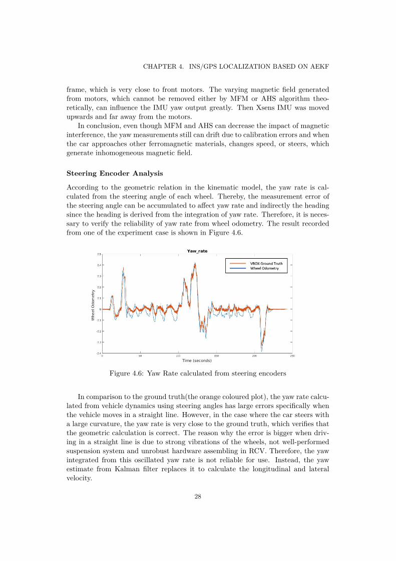
According to the geometric relation in the kinematic model, the yaw rate is cal-culated from the steering angle of each wheel. Thereby, the measurement error ofthe steering angle can be accumulated to affect yaw rate and indirectly the headingsince the heading is derived from the integration of yaw rate. Therefore, it is neces-sary to verify the reliability of yaw rate from wheel odometry. The result recordedfrom one of the experiment case is shown in Figure 4.6.

Figure 4.6: Yaw Rate calculated from steering encoders

In comparison to the ground truth(the orange coloured plot), the yaw rate calcu-lated from vehicle dynamics using steering angles has large errors specifically whenthe vehicle moves in a straight line. However, in the case where the car steers witha large curvature, the yaw rate is very close to the ground truth, which verifies thatthe geometric calculation is correct. The reason why the error is bigger when driv-ing in a straight line is due to strong vibrations of the wheels, not well-performedsuspension system and unrobust hardware assembling in RCV. Therefore, the yawintegrated from this oscillated yaw rate is not reliable for use. Instead, the yawestimate from Kalman filter replaces it to calculate the longitudinal and lateralvelocity.

28

4.4. IMPLEMENTATION

GPS Property Analysis

Trimble GPS without RTK is used for research on GPS oscillation. With the currentconfiguration from previous work, the GPS positioning is varying within 0.5m inthe open environment, where signals from many satellites are received in goodcondition. However, due to its sensitivity to the satellite geometry, GPS positioningcan oscillate in a large scale in dense urban areas.

Reach GPS with RTK supported can position a vehicle precisely but it dependson the GPS status in the receiver. With the configuration of “GPS + GLONASS +GALILEO + SBAS + QZSS” pack and only 5 Hz sampling frequency, it works wellat “Fix” or “Float” status and can reach the measurement accuracy to centimeterand decimeter respectively. However, Reach GPS is fragile to the case of reflectivebuildings due to its single-frequency receiver. Therefore, it is impossible to createa differential GPS scenario by twin Reach RTK GPS to provide absolute headingangle referenced by global north.

Xsens GPS also outputs position which is processed by vehicle odoemtry in-sides Xsens IMU. Observed from the tests, its position estimates are smoother thanTrimble GPS after filtering in Xsens but it has a considerable bias comapred to theground truth.

4.4.2 Sensor Placement

Figure 4.7: Sensor Placement on RCV

1O - ZED camera2O - Dual antenna of VBOX 3i3O - antenna of Trimble or Reach GPS4O - Xsens IMU5O - Speed encoder6O - Steering encoder

29


Figure 4.7 demonstrates the places where sensors are attached to the RCV. Theantenna either of VBOX 3i or Reach GPS should be hung over the vehicle in orderto receive the GPS signal better. Previously, Xsens IMU was placed at center of theRCV chassis, which means IMU was completely exposed to the strong magnetic fieldgenerated from RCV, such as motors, cables, and material. This can easily distortthe magnetometer, resulting in incorrect measurements. Having been re-attachedto the top and away from the motors in RCV, Xsens IMU performed much betterdue to declined magnetic interference from RCV. The ZED camera was fixed facingforward with a good sight to obtain as many visual features as possible to be usedin visual odometry.

4.4.3 Software Platform

The software design is operated in the environment, ROS(Robot Operating System)on Ubuntu 16.04.5 LTS. The AEKF, EKF and UKF algorithm are programmed inC++ and python supported by ROS. The software framework is supported by theROS package robot_localization. And the computing platform is a MSI G Series,Core i7 Laptop with GPU supported. The computer works as one of the nodesdistributed in the Ethernet network and bridges the communication from dSpace.The data communication in RCV is indicated in figure 4.8.

Figure 4.8: Data Communication in RCV

RCV real-time software structure basically can be divided into the lower andupper layer. In the low layer, the computational unit, dSpace autobox, is responsiblefor monitoring the state of RCV, including speed, steering, acceleration through

30

4.4. IMPLEMENTATION

CAN communication, and low-level motor controlling. The IMU and encoder dataare collected in lower layer and packed to multiple messages broadcast to the upperlayer through UDP protocol. Then, the functions of environmental perception andstrategy decision, such as localization and path planning, are realized in upperlayer where lidar, camera, and GPS are connected to ROS via Ethernet. Moreover,the communication between low and upper layer has limited delays and good datasynchronization in practice, which is important to secure the frequency of eachsensor message used for data fusion.

4.4.4 Coordinate Transform

Coordinate System

Each sensor has its own frame with respect to the RCV body-fixed frame. Thetransformation between these frames is supported by tf ROS package. The relationbetween each sensor frame and body-fixed frame is demonstrated in Figure 4.9,which is identical to the frame map exported from rqt_tf_tree.

Figure 4.9: Rqt Frame Tree

31


REP105, the standard of coordinate frames for mobile platforms used by ROS,specifies three principal frames: map, odom, and base_link. Base_link frame isfixed to the vehicle and usually locates the origin in the center of the mass. Odomframe can be drifting due to the definition by motion, such as wheel odomety andvisual odometry. While map frame, similar to odom frame, is a world fixed framebut provides stable reference to the pose of the vehicle. Generally, the origins ofthree frames are aligned before the vehicle starts moving. Moreover, they have thetransformation from one to another: map frame -> odom frame -> base_link frame.In addition, each sensor has its own frame correlated to the base_link frame, whichis shown in the figures above. The transformation amongst all frames is broadcastin certain frequency by tf package.

In order to integrate GPS data into fusion, the conversion from UTM frame tomap/odom frame is necessary. Note that GPS position has already been convertedto UTM format by Trimble or Reach GPS receiver. UTM frame points the x-axis toeast and y-axis to north with z-axis up. In 2D space, the coordinate transformationfrom UTM frame to map/odom/base_link frame can be described in Figure 4.10.

Figure 4.10: GPS coordinate Transform

As can be seen in Figure 4.10, the map, odom, and base_link frame are ini-tialized to be aligned at the beginning. It is also obvious to find that the transfor-mation from UTM to odom coordinate can be realized through the translation by(xutm,yutm) and the rotation by θ.

The transformation equation from UTM to odom coordinate is indicated asbelow (in 3D space):

32

4.4. IMPLEMENTATION

T =

cosθycosθz cosθzcosθxsinθy − cosθxsinθz cosθzcosθxsinθy + sinθxsinθz xUT M0

cosθysinθz cosθxcosθz + sinθxsinθysinθz −cosθzsinθx + cosθxsinθysinθz yUT M0

−sinθy cosθysinθx cosθxsinθy zUT M0

0 0 0 1

xodom

yodom

zodom

1

= T−1

xUT Mt

yUT Mt

zUT Mt

1

(4.20)

In 2D space:

T =

cosθz −sinθz xUT M0

sinθz cosθz yUT M0

0 0 1

xodom

yodom

1

= T−1

xUT Mt

yUT Mt

1

(4.21)

In equations (4.20), θx, θy, and θz are the vehicle’s initial UTM-frame roll, pitch,and yaw respectively. xUT M0 , yUT M0 , and zUT M0 are the initial GPS positions ofa vehicle with respect to the UTM coordinate.

In order to transform GPS data from UTM to local coordinate, it is necessaryto have both translational and rotaitonal relation between two coordinates. It isstraightforward to obtain the translation distance, which is related to the initialposition of point O with respect to UTM coordinate. However, it is impossibleto use magnetometer to measure the rotational relation since the magnetometer isdistorted by magnetic interference generated from RCV. In order to cope with thisproblem, another solution comes up.

In 2D space:

xodom

yodom

1

=

cos(θz + ε) −sin(θz + ε) xUT M0

sin(θz + ε) cos(θz + ε) yUT M0

0 0 1

−1 xUT Mt

yUT Mt

1

(4.22)

The offset ε, which corresponds to θ in figure 4.10, needs to be obtained at the begin-ning in order to rotate UTM coordinate to local coordinate. The solution is to drivethe vehicle forward for about 2 meters. During this distance, several pairs of pointsare recorded both in UTM and odom coordinate, such as the pair of points A,Bwith coordinates (xAutm, yAutm), (xAodom, yAodom), and (xButm, yButm), (xBodom,yBodom). Then, those points’ coordinates are given as inputs to matrix equation(4.22). Since the equation only contains four unknown parameters θz, ε, xUT M0 ,yUT M0 , four equations are sufficient to derive those parameters and transformationmatrix T .

33


4.4.5 Filter parameters & settings

The frequency of each message

The frequency of each observation message read from sensors is shown in Table 4.1.

Table 4.1: Message frequency

Message FrequencyWheel Odometry 25 HzVisual Odometry 15 Hz

GPS Mapped to Odometry 5 HzIMU 30 Hz

Estimator 30 Hz

The estimator should work at sufficiently high frequency in order to fulfill therequirement of control system in RCV. Moreover, Whichever measurement mes-sage(either GPS, IMU or wheel odometry) reaches the estimator, the estimator willprocess the latest data. Therefore, it is reasonable to set the frequency of the esti-mator much higher than any measurement message. GPS frequency can be slightlylow since a estimator with good motion model does not require high-frequency cor-rection to the position. Visual Odometry is re-sampled to limit the frequency to 15Hz due to limited computational property of CPU.

Motion Model and State Vector

Since only the state of the vehicle in 2D is estimated, the dimension of state vectorcan be cut down to 1×8 after vertical velocity, roll and pitch angle are removed.

StateX =[posx posy vx vy ax ay θz θz

](4.23)

In the state vector, θz, posx and posy denote global yaw and position in the localmap, while vx, vy, ax, ay and θz represent the velocity, acceleration, and yaw ratewith respect to the body-fixed frame.

On the prediction stage, AEKF works the same as EKF and linearize the motionmodel, which is shown in equation (4.24).

34

4.4. IMPLEMENTATION

1 0 cosθz∆t sinθz∆t 12cosθz∆t2 1

2sinθz∆t2 0 00 1 sinθz∆t cosθz∆t 1

2sinθz∆t2 12cosθz∆t2 0 0

0 0 1 0 sinθz∆t cosθz∆t 0 00 0 0 1 cosθz∆t sinθz∆t 0 00 0 0 0 1 0 0 00 0 0 0 0 1 0 00 0 0 0 0 1 ∆t 00 0 0 0 0 0 0 1

(4.24)

Note that ∆t denotes the time instance, which corresponds to the frequency ofthe estimator. The observation model is simpler only by assigning the measurementvalue to the corresponding element in the state vector.

Observation Input

Unreliable observations should not be used for the estimator. For example, as isdiscussed before, the yaw rate derived from wheel odometry has a great bias dueto mechanical vibrations on the wheel axle, therefore the yaw and yaw rate shallbe removed from the sensor fusion. Consequently, only the longitudinal and lateralvelocity from wheel odometry are utilized by the Kalman filter. The list of eachobservation input to the estimator is shown in Table 4.2.

Table 4.2: Observation Input

Observation Input (odom frame) Input (base_link frame)Wheel Odometry - vx, vy

Visual Odometry yaw yaw rateGPS Mapped Odometry posx, posy -

IMU yaw yaw rate, ax, ay

Regarding the implementation on ROS system, all observation messages shouldbe pre-processed to odom and base_link frame before being fused in the Kalmanfilter. In details, the longitudinal and lateral velocity vx and vy need to be attachedto base_link frame, as well as the accelerations ax and ay. The GPS positionmessage should be converted from the map frame to odom frame, which is describedas GPS mapped odometry in the above table.

35


4.5 Experiment Results

4.5.1 Algorithm Performance on Good GPS Condition

Testing Road

Figure 4.11: Testing Track

Figure 4.11 depicts the road used for the algorithm testing. The driving directionis from point A to point F, that is to say, A - B - C - D - E - F. The track includestwo straight road segments A - B - C and E - F, and one tight turning C - D - E.It can verify the algorithm performance on different nonlinear levels. Moreover, theroad segment C - D - E is a slope with gradient around 0.2, while other segments,such as A - B - C and E - F, can be considered as flat roads with 0.07 gradient.

Yaw Estimation

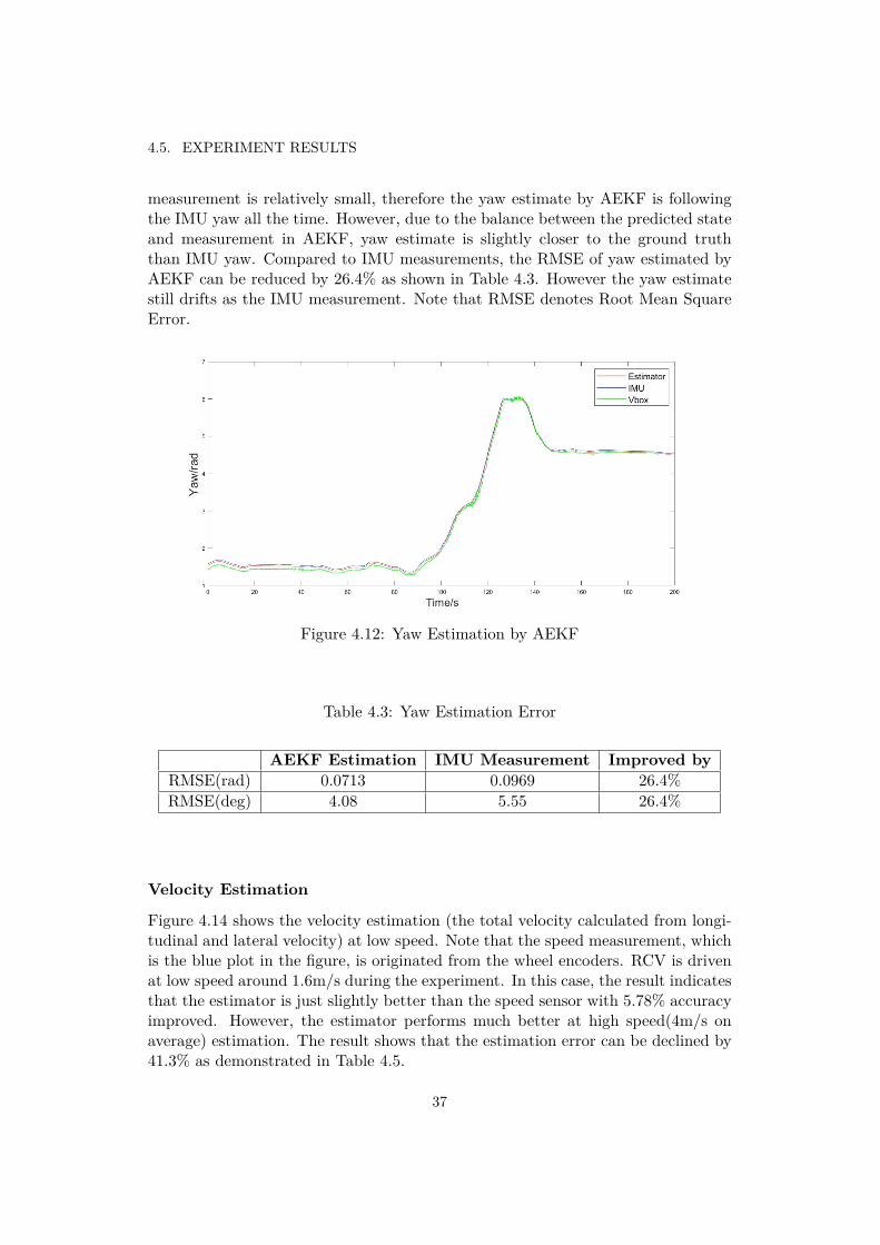
Figure 4.12 demonstrates the result of yaw estimation by the AEKF-based esti-mator. The red plot represents the yaw estimate while the blue one comes fromthe yaw measurement by IMU. The Green plot from VBOX, is able to provide theground truth of heading according to 0.1◦/0.0017 rad accuracy specified in VBOXdatasheet. It is obvious to see that the yaw measurement has a bias 11◦/0.2 radinitially due to the calibration error. GPS/IMU navigation system only relies onIMU yaw measurements to correct the heading estimate and the covariance for IMU

36

4.5. EXPERIMENT RESULTS

measurement is relatively small, therefore the yaw estimate by AEKF is followingthe IMU yaw all the time. However, due to the balance between the predicted stateand measurement in AEKF, yaw estimate is slightly closer to the ground truththan IMU yaw. Compared to IMU measurements, the RMSE of yaw estimated byAEKF can be reduced by 26.4% as shown in Table 4.3. However the yaw estimatestill drifts as the IMU measurement. Note that RMSE denotes Root Mean SquareError.

Figure 4.12: Yaw Estimation by AEKF

Table 4.3: Yaw Estimation Error

AEKF Estimation IMU Measurement Improved byRMSE(rad) 0.0713 0.0969 26.4%RMSE(deg) 4.08 5.55 26.4%

Velocity Estimation

Figure 4.14 shows the velocity estimation (the total velocity calculated from longi-tudinal and lateral velocity) at low speed. Note that the speed measurement, whichis the blue plot in the figure, is originated from the wheel encoders. RCV is drivenat low speed around 1.6m/s during the experiment. In this case, the result indicatesthat the estimator is just slightly better than the speed sensor with 5.78% accuracyimproved. However, the estimator performs much better at high speed(4m/s onaverage) estimation. The result shows that the estimation error can be declined by41.3% as demonstrated in Table 4.5.

37


Figure 4.13: Estimation at Low Speed

Table 4.4: Estimation Error at Low Speed

Low Speed AEKF Estimation Speed Sensor Improved byRMSE(m/s) 0.0669 0.0710 5.78%RMSE(km/h) 0.241 0.256 5.78%

Figure 4.14: Estimation at High Speed

Table 4.5: Estimation Error at High Speed

High Speed AEKF Estimation Speed Sensor Improved byRMSE(m/s) 0.141 0.240 41.3%RMSE(km/h) 0.508 0.864 41.3%

38


Position Estimation

As is demonstrated in Figure 4.15, the estimated path almost overlaps GPS path.This verifies that the estimator works correctly on position estimation when GPSis in good condition since there is no conflict between the predicted position andthe measured postion by GPS. However, the position estimate of point D in figure4.11 is a bit diverged from the GPS position because of the slope at point D. Tobe more specific, this is because that only 2D position is under estimation withoutconsideration of pitch angle. Therefore, either longitudinal or lateral velocity pro-jected on x axis (the horizontal axis of the map frame) is higher than true velocitywhen the vehicle moves downhills, which can result in difference from GPS. How-ever, AEKF adaptively increases the process noise based on innovation in a highnon-linear situation, such as on the road with high curvature as point D. Therefore,the weight of the prediction is degraded and the measurement correction becomesmore dominant. This can slightly help decrease the linearizaition error, which willbe discussed more in the following sections.

Figure 4.15: Position Estimation by AEKF

39


Yaw Rate Estimation

In the estimator, yaw rate is only corrected by yaw rate measured by gyroscopein IMU. Therefore, the yaw rate estimated by AEKF is supposed to be similar tothe yaw rate output from Vbox. Here, Figure 4.16 compares the yaw rate estimatefrom AEKF and the yaw rate measured by vbox. As is deciphered from the figure,it is obvious that the yaw rate from AEKF and from Vbox are indeed close to eachother.

Figure 4.16: Yaw Rate Estimation by AEKF

4.5.2 Localization on GPS OscillationTest Road

The Test Road is selected for special requirements that are under GPS oscillation.The GPS oscillation can happen when RCV is driven in dense regions with crowdedbuildings located. Therefore, during this experiment, RCV runs across the KTHcampus and follows the direction zone A - B - C, which is also expressed by yellowarrows in Figure 4.17(a). Figure 4.17(b) shows the GPS positioning by TrimbleGPS from zone A to B to C, corresponding to the left figure. In figure 4.17(b),red plot is the ground truth of the path where the vehicle is actually driven, whileblue plot represents the GPS signal on the road. The ground truth is derivedfrom GPS regression due to the property of Trimble GPS that can measure theposition precisely within 0.5 meter in open environments (with many satellites)but oscillates under bad GPS condition. This ground truth can be verified to beuseful by comparing with the driving line predetermined on the map. Although thisground truth might be weak to specify the accuracy of AEKF, it can be sufficientto compare amongst AEKF, EKF, and UKF.

40


It is obvious to observe that zone A, zone C pointed out with green circles in4.17(a) are the areas where GPS signal oscillates very much. Although zone B isalso encompassed by beside buildings, it only causes slight GPS fluctuation since thebuildings around there are relatively low. The sensor data is recorded in real timeduring the experiment and used for comparing the algorithm performance offlinebetween AEKF, EKF, and UKF. These three algorithms are compared based on thesame basic parameters configured, including the working frequency of the estimator,sampling frequency of sensors, initial covariance of GPS noise and process noise, theoutlier threshold, and measurement covariance of IMU and wheel odometry.

(a) Test Road (b) GPS Signal

Figure 4.17: GPS Signal on the Test Road

Result

AEKF, EKF and UKF algorithm are applied to localize RCV based on the samedataset. Through the test on Trimble GPS in the open environment, the positionmeasurement varied wihin 0.5 meter, which derives 0.25m2 measurement covarianceof either position x or y in good GPS condition. The GPS position can oscillatearound 1 meter when GPS condition is slightly bad. Therefore, in the experiment,different covariances(0.25m2 and 1.0m2) are configured for EKF and UKF com-pared to the covariance of 0.25m2 initialized for AEKF. Moreover, the Mahalanobis

41


threshold [18] is set to be 4, which is the optimal value for EKF by tuning. Theresults of position estimate by EKF are shown in Figure 4.18.

(a) σ2 = 0.25 (b) σ2 = 1.0

Figure 4.18: Position estimation by EKF

The Results of UKF-based localization with covariance of 0.25m2 and 1.0m2 aredemonstrated in figure 4.19.

(a) σ2 = 0.25 (b) σ2 = 1.0

Figure 4.19: Position estimation by UKF

In order to guarantee the same precondition between EKF and UKF, the co-

42


variance of 0.25meter2 is set to the GPS measurement covariance of position x ory for AEKF based localization initially. The result is shown in Figure 4.20.

Figure 4.20: Position Estimation by AEKF (initial σ2 = 0.25)

The AEKF-based estimator estimates the covariance of position measurementsand process noise in real time based on the residual and innovation. The covarianceof distance measurements, which is calculated by square root of the sum of thesquares of positions x, y, is plotted in Figure 4.21.

Figure 4.21: Position Estimation by AEKF

There are three zones A, B, and C addressed in the figure, which corresponds

43


to Figure 4.17(a). The distance covariance of zone B is specifically zoomed in tobe more visible. In addition, The red lines aligned on the time axis represents themoments when GPS outliers are classified out. As well as Mahalanobis threshold[18],the threshold of 90.25m2 is added to constrain the outliers becuase the TrimbleGPS receiver, that has C/A-code, L1/L2 supported, measures the position withhorizontal uncertainty of 19 meters (95%) in the worst case according to Table 2.2.Thereby, assuming the current distance covariance estimated by AEKF is higherthan 90.25m2, the GPS measurement should be categorized to an outlier. Besides,provided the current GPS measurement is an outlier, the distance covariance inheritsthe covariance from the last estimate. That is the reason why there are multiplehorizontal blue lines appearing in Figure 4.21 from time to time.

The comparison among the accuracy of AEKF, EKF, and UKF by root meansquare errors is clarified in Table 4.6.

Table 4.6: Position Estimation Error (AEKF, EKF, and UKF)

AEKF EKF(σ2=0.25) EKF(σ2=1.0) UKF(σ2=0.25) UKF(σ2=1.0)RMSE(m2) 0.8630 1.8657 3.0689 2.3015 1.4406

In conclusion, AEKF based algorithm improves the position accuracy by 53.74%compared to EKF and 40.09% compared to UKF under GPS oscillation.

4.6 DiscussionAEKF performs similarly to EKF when GPS is in good condition. It can improvethe accuracy of heading and velocity. In Figure 4.12, the heading measured by IMUhas a bias at the beginning due to calibration errors and this bias was varying dueto the inhomogeneous magnetic field varying on the road. The yaw measurementis balanced with the yaw from the predicted state to obtain more accurate headingestimate but still can drifts away from the ground truth. As for the velocity esti-mation, AEKF can provide much better estimate than wheel odometry especaillyat higher speed. There are mainly two reasons able to explain this result. On onehand, the wheel encoders attached to the wheel axles vibrate much more when RCVis running faster. On the other hand, kinematic model can describe the vehicle statebetter at lower speed according to the paper [30].

AEKF can smooth the estimated path. By comparing the position estimate inthe zone B. which is zoomed in Figure 4.18(a), 4.19(a), and 4.20 on purpose, thepath estimated by AEKF has less oscillations due to the adaptive update on thecovariance. As for EKF or UKF, the covariance is a fixed value, that may forcethe estimator to trust the GPS measurement all the time, especially when the GPSmeasurement is not categorized into an outlier but just slightly fluctuates around 1meter. Differently, AEKF estimates the GPS covariance based on residual and the

44

4.6. DISCUSSION

covariance from past estimated states. The forgetting factor, which is introduced inprevious sections, can control the impact from past covariance estimates and helpreject the sudden covariance change, which indirectly smooths the path. Generally,the smaller the forgetting factor is set, the smoother the path can be. In theexperiment, the forgetting parameter for GPS covariance estimate is 0.4, so thatnot only the estimated path can be smoothed, but also the latest GPS measurementcan be made use of. Note that the process noise covariance should be estimated asalong as GPS covariance updates. Therefore, the forgetting factor for process noiceis optimally tuned to be 0.85 based on the value 0.4 for GPS covariance estimate.

By Comparing the robustness to outliers in zone A and zone C through Figure4.18, 4.19, and 4.20, AEKF outperforms either EKF of UKF algorithm. The GPSsignals within zone A and zone C have great divergences that ought to be classifiedas outliers and removed from data fusion in Kalman filter. Figure 4.22 demonstrateshow EKF works when GPS outliers appears. In the figure, the vehicle (describedas the blue points) is moving straightforward while GPS signal (described by thered points) deviates for a while but recovers to a good measurement afterwards.The ellipses around the red points represent GPS covariances and the blue ellipsesrepresent the covariances of the current estimated state. The red ellipses alwaysmaintain the same size due to unchanged covariance configured in EKF. Moreover,the Mahalanobis distance threshold is also used to constrain the outlier by compar-ing the Mahalanobis distance calculated from the covariance of the predicted stateand the GPS covariance. With this threshold applied, if either the predicted stateor GPS measurement has a larger covariance/uncertainty, the GPS measurementwill be more likely to be classified as an inlier, which affects the position estimateto approach GPS signal. Therefore, as can be seen in Figure 4.22, the positionestimate of the vehicle always varies along with the GPS position due to the largeGPS covariance fixed.

Figure 4.22: Covariance Estimation by EKF

Figure 4.23 shows the adaptive covariance update by AEKF on the same con-dition as EKF. The GPS covariance in each sampling time is updated based on theweighted average of the current residual and previous GPS covariance, which canlead to small GPS covariance under good GPS condition, such as the beginningin the figure. Similarly, the innovation-based covariance of process noise is also

45


changed to be small. In contrast to EKF, AEKF compares Mahalanobis thresh-old with the distance calculated from the last GPS covariance and the covarianceof predicted state. Therefore, at the moment that GPS suddenly oscillates, thisinstant change can be more likely to be classified to an outlier due to small GPScovariance estimated in last step. However, as can be observed, there is a smallspike in zone A in Figure 4.20, which corresponds to the covariance rising up to70m2 in zone A in Figure 4.21. This phenomenon can also be explained by Figure4.23. Although outliers can be detected once GPS suddenly fluctuates and removedaway, the covariance of the state estimate can still increase due to the accumulationfrom process noise. Therefore, there will exsit a moment when the state covarianceis great enough to enable the GPS signal to be acceptable as an inlier for AEKF.After this moment, the GPS covariance can be updated again and scales up the po-sition estimate. Therefore, it can be concluded that AEKF is more sensitive to GPSoutliers than EKF or UKF but becomes less effective for long-term GPS outage.

Figure 4.23: Path Estimation by AEKF

In conclusion, AEKF based algorithm fusing GPS, IMU and Wheel odometrycan precisely estimate the vehicular state, including velocity, yaw and yaw rate. Aswell as the well-performed localization in good GPS condition by AEKF, AEKFalgorithm has more robustness to GPS oscillation and outage compared with EKFand UKF.

46

Chapter 5

Vision-aided Heading Estimation

Differet from IMU, visual odometry is independent to magnetic field. Therefore itmay provide better heading measurements than IMU under magnetic interference.Visual odometry computes the relative motion between neighbour image framesand integrate to calculate the heading, which also has a drifting due to relativerotational errors accumulated all the time. Therefore, the visual odoemtry computesthe heading based on the current heading estimate from the estimator added bythe rotational angle from image matching in stead, which is similar to the wheelodometry. In this thesis project, ZED camera, which is a calibrated stereo camera,is used for the implementation of visual odometry.

5.1 Algorithm Introduction

The stereo visual odometry implemented in this thesis is supported by libviso2library[29][37], proposed by Geiger Andreas, et al. In the thesis project, the researchon visual odometry algorithm is not a main focus, so only a brief introduction ofthe algorithm is given in this chapter.

The workflow of the stereo visual odometry can be divided into two steps: featurematching and egomotion estimation. The first stage is to match the image featuresbetween four images, which are the left and right images of two consecutive frames.The method of NMS(Non-maximum Suppression) is employed to extract the featurecandidates in order to save the computational cost. All features are sorted out tofind the best matches and outliers are removed by the epipolar constraint.

After the feature matches obtained from the previous step, the camera motioncan be computed by minimizing the sum of reprojection erros and refining theobtained velocity estimates by a Kalman filter. The features from the previousframe can be projected into 3D space given calibration parameters of the stereocamera. After that, these 3D points can be reprojected to the current image frame,which is shown in equation (5.1).

47

CHAPTER 5. VISION-AIDED HEADING ESTIMATION

uv1

=

f 0 cu

0 f cv

0 0 1

+ ([R t

] XYZ1

−S0

0

) (5.1)

Here the first 3×3 matrix on the right side is a camera intrinsic matrix, and cu

and cv are the coordinate of a principal point of the image. [u v 1]T and [x y z 1]T arethe homogeneous coordinates of a 2D image point and 3D point after projection. [Rt] is the transformation matrix, where R is a rotation matrix and t is a translationvector. The shift S is 0 on the left image and equal to baseline on the right image.

After the transformation, the 3D feature points from the previous frame aremapped into 2D to the current image coordinate. Then Gauss-Newton optimizationmethod is employed to iteratively minimize the value calculated by equation (5.2).

n∑i=1|x(l)

t − x(l)t−1|

2+|x(r)t − x

(r)t−1|

2 (5.2)

Note that x(l)t is the feature point’s coordinate in the current left image frame,

and x(l)t−1 is the coordinate of a 2d point by reprojection on the current left image

frame from the previous image. Similarly, x(l)t and x(l)

t−1 represent the pair on theright images. During the iteration, the method Random Sample Consensus is im-plemented to classify the inliers for refining the parameters and yielding the finalrotation and translation matrix.

5.2 Yaw Rate TestThe heading estimated by visual odometry is derived from the image rotation basedon the previous heading estimate. The yaw accuracy can be verified by the yawrate indirectly. Figure 5.1 and Table 5.1 compare the yaw rate estimate betweenvisual odometry and wheel odometry. The yaw rate is tested on the same test trackin Figure 4.11.

Table 5.1: Yaw Rate Estimation Error between VO and WO

Visual Odometry Wheel Odometry Improved byRMSE(rad/s) 0.016 0.030 46.7%RMSE(deg/s) 0.917 1.72 46.7%

48

5.3. RESULTS AND DISCUSSION

Figure 5.1: Yaw Rate Test between VO and WO

As is deciphered from the figure and table, visual odometry can perform betterthan wheel odometry by 46.7% regarding the yaw rate measurement. Because ofstrong vibration of encoders and limiation of kinematic model at high speed, theyaw rate calculated by wheel odometry has an error up to 5 deg/s in the worstcase, which cannot be used for the estimator. By contrast, visual odometry, whichis independent to physical noise and modelling error, outperforms to measure therotational movement.

5.3 Results and Discussion

The vision-aided heading estimation is tested under the same precondition as thetest of algorithm performance on good GPS condition, such as the same test track,road condition, and approximately the same magnetic interference. For the sakeof comparison, the basic parameters are configured to be identical, such as IMUmeasurement covariance and the process noise of yaw rate. However, In order tobalance the heading measurement between IMU and visual odometry, the IMUfrequency is resampled down to 15 Hz, which is equivalent to the visual odometry’sfrequency, and the covariance of visual odometry is set equal to the IMU covariance.The result of heading estimation with vision aided is shown in Figure 5.2 and Table5.2.

49

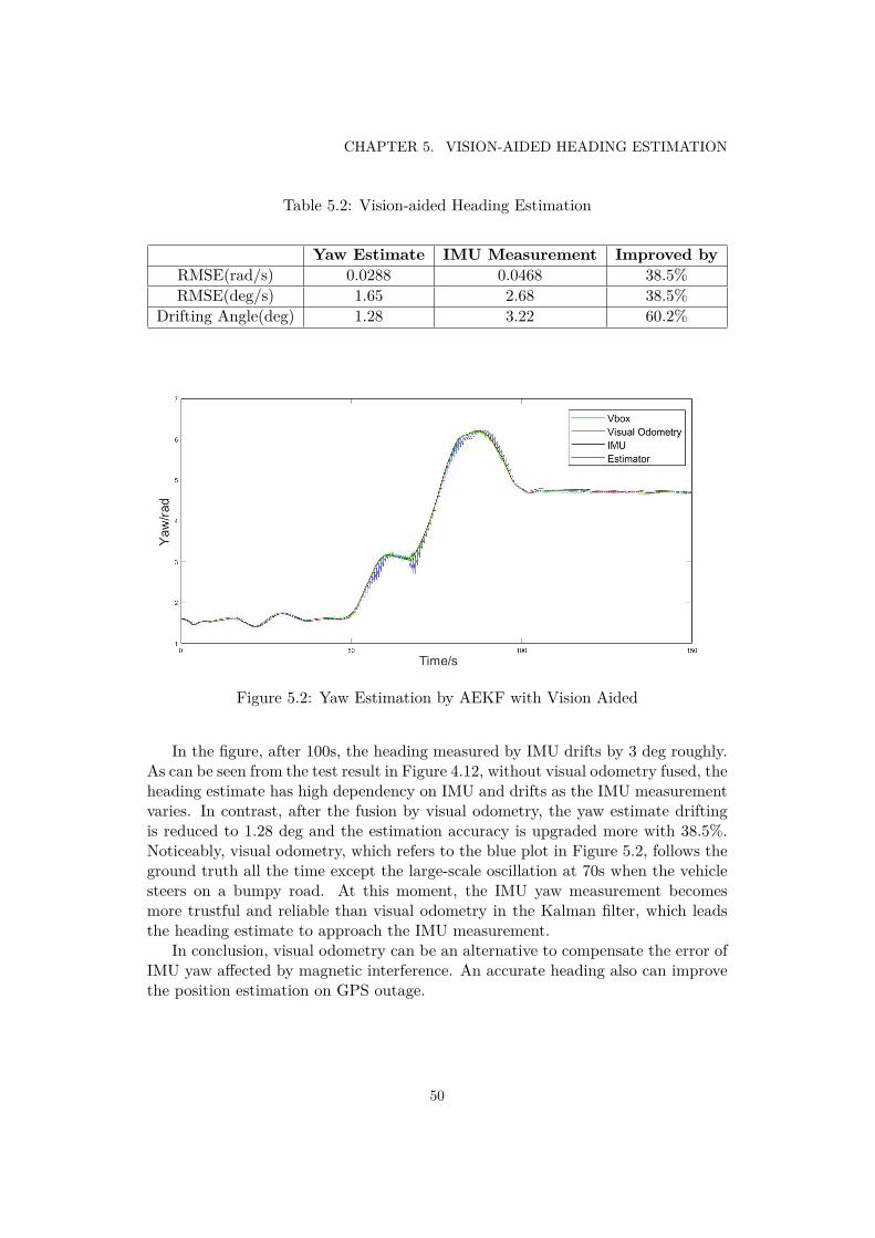
CHAPTER 5. VISION-AIDED HEADING ESTIMATION

Table 5.2: Vision-aided Heading Estimation

Yaw Estimate IMU Measurement Improved byRMSE(rad/s) 0.0288 0.0468 38.5%RMSE(deg/s) 1.65 2.68 38.5%

Drifting Angle(deg) 1.28 3.22 60.2%

Figure 5.2: Yaw Estimation by AEKF with Vision Aided

In the figure, after 100s, the heading measured by IMU drifts by 3 deg roughly.As can be seen from the test result in Figure 4.12, without visual odometry fused, theheading estimate has high dependency on IMU and drifts as the IMU measurementvaries. In contrast, after the fusion by visual odometry, the yaw estimate driftingis reduced to 1.28 deg and the estimation accuracy is upgraded more with 38.5%.Noticeably, visual odometry, which refers to the blue plot in Figure 5.2, follows theground truth all the time except the large-scale oscillation at 70s when the vehiclesteers on a bumpy road. At this moment, the IMU yaw measurement becomesmore trustful and reliable than visual odometry in the Kalman filter, which leadsthe heading estimate to approach the IMU measurement.

In conclusion, visual odometry can be an alternative to compensate the error ofIMU yaw affected by magnetic interference. An accurate heading also can improvethe position estimation on GPS outage.

50

Chapter 6

Conclusion and Future Work

In this chapter, I summarized the thesis work. Meanwhile, some suggestions for thefuture work are also briefly discussed.

6.1 Conclusion

In this thesis, a multi-sensor based localization and odometry estimation algorithmis proposed. There are two principal focuses: localization on GPS oscillation andheading estimation under magnetic interference. In order to improve the robustnessto GPS fluctuation due to the urban environment, AEKF is implemented to adapa-tively estimate the covariance of GPS measurement and process noise. Through theexperiments, AEKF is proved to be able to localize the vehicle more consecutivelyon GPS oscillation and has higher sensitivity to GPS outliers, compared to tradi-tional Kalman filters, EKF and UKF. Apart from the localization, AEKF can alsoimprove the odometry estimation by fusing GPS, IMU, and encoders. Both speedand heading can be estimated more accurately than merely sensor measurements,especially when the speed is high. The heading estimated by AHS algorithm inXsens IMU is interfered by the magnetic field from the external environment andRCV itself. In order to decrease the drifting error of IMU heading, stereo visualodometry is implemented and verified to be useful.

Through the experiment results, the answers to research questions are clarifiedbelow:

Question: Through some experiments, can AEKF (Adaptive Extended KalmanFilter) outperform CEKF (Conventional Extended Kalman Filter) and UKF (Un-scented Kalman Filter) in terms of estimation accuracy, and robustness to GPSoscillation and outage?

Answer: Yes. In the environment of GPS oscillation and outage, AEKF canestimate more consecutive and accurate position than CEKF and UKF with 53.74%and 40.09% improved respectively in the experiment.

Question: Can visual odometry improve the accuracy and constrain the driftingerror of heading estimate due to magnetic interference?

51

CHAPTER 6. CONCLUSION AND FUTURE WORK

Answer: Yes. Without visual odometry fused into Kalman filter, the headingestimate almost drifts as IMU yaw and only improves the heading accuracy by 26.4%compared to IMU measurements. However, due to assistant by visual odometryunder magnetic interference, the heading estimate error due to IMU drfiting canbe more constrained, which results in 38.5% accuracy improved compared to IMUmeasurements.

6.2 Future WorkThe future work is mainly to improve the performance of the localization systemof the RCV from both hardware and software perspectives, which are discussed asbelow:

6.2.1 More Robust Sensor AssemblyThe camera and steering encoders should be fixed rigidly to the RCV. Otherwise,the vibration of RCV can distort the visual odometry and introduce a lot of noisein steering angle respectively. If the steering encoder can provide better anglemeasurement, the velocity can be better calculated through geometric relationshipinstead of using the average measurement of speed encoders.

6.2.2 More Extensive Parameter TuningThe IMU measurement covariance set in the Kalman filter is originated from thespecialization document of the product. However, the performance of IMU mea-surements depends on how well the sensor is calibrated. It is also possible to tunethe process covariance for a better state estimation.

6.2.3 Dynamic Vehicle ModelThe kinematic model is a good modeling for a low-speed vehicle. The software istested at the speed under 10km/h, which is a low-speed test. It would be valuableto test on high speed and compare with the dynamic model.

6.2.4 Implementation of dual GPS systemThe dual GPS system is very valuable to integrate to provide absolute headingmeasurement. Even though visual odometry can improve the heading estimation,yaw estimate still relies on the IMU heading to constrain the drifting. Therefore,for the sake of a long-term navigation, dual GPS system is highly recommended tobe utilized. Moreover, it is also of great significance to isolate the IMU better fromthe electromagnetic interference generated from the electric motors in RCV.

52

Bibliography

[1] https://www.sae.org/standards/content/j3016_201609/ (accessed: 2018-03-01)

[2] https://nordic.businessinsider.com/tesla-model-3-best-features-2017-6?r=USIR=T (accessed: 2018-03-01)

[3] https://www.youtube.com/watch?v=a-hvCL1y7ME (accessed: 2018-03-06)

[4] Petter Tomner. Design and implementation of control and actuation for an over-actuated research vehicle. Master’s thesis, KTH, Vehicle Dynamics, 2015.

[5] https://kth.instructure.com/courses/4962/pages/module1-mtrl-sensing, Shortcalculation of impact of a gyro biasPreview the document (accessed: 2018-04-11)

[6] https://base.xsens.com/hc/en-us/articles/211809465-Active-Heading-Stabilization-AHS- (accessed: 2018-03-14)

[7] https://base.xsens.com/hc/en-us/articles/213588029-In-run-Compass-Calibration-ICC-and-Representative-Motion (accessed: 2018-03-14)

[8] https://base.xsens.com/hc/en-us/articles/115000888529-How-to-perform-a-Magnetic-Field-Mapper-MFM-with-the-MVN-Awinda (accessed: 2018-03-14)

[9] https://en.wikipedia.org/wiki/GPS (accessed: 2018-03-14)

[10] https://support.strava.com/hc/en-us/articles/216917707-Bad-GPS-Data-What-Why-Howwhy (accessed: 2018-03-14)

[11] Andras, K. (1999). Role of the Geometry in GPS Positioning. Periodica Poly-technica SER. CIV. ENG. Vol.43, NO.1, PP. 43-53

[12] https://www.novatel.com/an-introduction-to-gnss/chapter-5-resolving-errors/real-time-kinematic-rtk/ (accessed: 2018-03-14)

[13] https://www.stereolabs.com/zed/ (accessed: 2018-04-11)

[14] https://www.vboxautomotive.co.uk/index.php/en/products/data-loggers/vbox-3i-dual-antennaspecs (accessed: 2018-03-06)

53

BIBLIOGRAPHY

[15] Wan, E., Van Der Merwe, R. (2000). The unscented Kalman filter for nonlin-ear estimation. Adaptive Systems for Signal Processing, Communications, andControl Symposium 2000. AS-SPCC. The IEEE 2000, 153-158.

[16] Akhlaghi, S., Zhou, N., Huang, Z. (2017). Adaptive adjustment of noise covari-ance in Kalman filter for dynamic state estimation. 2017 IEEE Power EnergySociety General Meeting, Chicago, IL, pp. 1-5.

[17] Reina, G., Vargas, A. (2007). Adaptive Kalman Filtering for GPS-based MobileRobot Localization. Safety, Security and Rescue Robotics, 2007. SSRR 2007.IEEE International Workshop on, 1-6.

[18] https://en.wikipedia.org/wiki/Mahalanobis_distance (accessed: 2018-03-21)

[19] https://gssc.esa.int/navipedia/index.php/RTK_Fundamentals(accessed:2018-03-21)

[20] Rezaei, S., Sengupta, R. (2007). Kalman Filter-Based Integration of DGPSand Vehicle Sensors for Localization. Control Systems Technology, IEEE Trans-actions on, 15(6), 1080-1088.

[21] Rudolph, V., Eric, A., (2004). Sigma-Point Kalman Filters for Nonlinear Es-timation and Sensor-Fusion-Applications to Integrated Navigation. Proceedingsof the AIAA Guidance, Navigation Control Conference. 3. 10.2514/6.2004-5120.

[22] Jeong W., Young-Joong K., Jeong-on L., Myo-Taeg L. (2006). Localizationof Mobile Robot using Particle Filter. SICE-ICASE, 2006. International JointConference, 3031-3034.

[23] St-Pierre, M., Gingras, D. (2004). Comparison between the unscented Kalmanfilter and the extended Kalman filter for the position estimation module of anintegrated navigation information system. Intelligent Vehicles Symposium, 2004IEEE, 831-835.

[24] El-Sheimy, N., Abdel-Hamid, W. (2007). A fuzzy-augmented Kalman filter forIMU/GPS integration. Journal of Applied Geodesy, 1(2), 91-102.

[25] Bistrovs, V., Kluga, A. (2013). The Analysis of the UKF-Based NavigationAlgorithm during GPS Outage. E LEKTRONIKA IR ELEKTROTECHNIKA,ISSN 1392-1215, VOL.19 , NO.10

[26] Mohamed, A., Schwarz, K. (1999). Adaptive Kalman Filtering for INS/GPS.Journal of Geodesy, 73(4), 193-203.

[27] Wang, J. (1999). Stochastic Modeling for Real-Time Kinematic GPS/-GLONASS Positioning. Navigation, 46(4), 297-305.

54

BIBLIOGRAPHY

[28] Kitt, B., Geiger, A., Lategahn, H. (2010). Visual odometry based on stereo im-age sequences with RANSAC-based outlier rejection scheme. Intelligent VehiclesSymposium (IV), 2010 IEEE, 486-492.

[29] Geiger, A., Ziegler, J., Stiller, C. (2011). StereoScan: Dense 3d reconstructionin real-time. Intelligent Vehicles Symposium (IV), 2011 IEEE, 963-968.

[30] Kong, J., Pfeiffer, M., Schildbach, G., Borrelli, F. (2015). Kinematic and dy-namic vehicle models for autonomous driving control design. Intelligent VehiclesSymposium (IV), 2015 IEEE, 1094-1099.

[31] Jiajun Shi, RCV Documentation, Integrated Transport Research Lab, 2018.

[32] https://en.wikipedia.org/wiki/Geodetic_datum (accessed: 2018-03-06)

[33] https://en.wikipedia.org/wiki/Universal_Transverse_Mercator_coordinate_system(accessed: 2018-03-06)

[34] https://en.wikipedia.org/wiki/ECEF (accessed: 2018-04-01)

[35] Yang, Y., Zhang, S. (2005). Adaptive fitting of systematic errors in navigation.Journal of Geodesy, 79(1-3), 43-49.

[36] N. Zhou, D. Meng, Z. Huang, G. Welch, "Dynamic state estimation using PMUData: a comparative study," IEEE Trans. Smart Grid, vol. 6, no. 1, pp. 450-460,Jan. 2015.

[37] http://www.cvlibs.net/software/libviso/ (accessed: 2018-05-03)

55

TRITA TRITA-ITM-EX 2019:10

www.kth.se

Documents

(VWLPDWLRQ - DiVA portal