Embed Size (px)
Citation preview

Computation of Turbulent Flows-State-of-the-Art, 1970 _:
by
w. C. Reynolds
Thermosciences DivisionDepartment of ·Mechanical Engineering
Stanford UniversityStanford, California
enw...........N
1.0-..J~O. ....,'"d(,).~
c::::(')!Xl!Xlc.net>ttl(')"-< c::lt"'ot-<
Ol;J;l......... 2:Nc.l-3t:1C1l
Z-..JWI....
~J
Prepared from work done under GrantsNSF-GK-10034 and
NASA-NgR-OS-Q20-420
Report MD·21
October 1970.(Reprinted February 1912)
Reproduced by \NATIONAL TECHNICAL "
INF~~~~!!5)o~'t~~~~ICESpringfield VA 22151
https://ntrs.nasa.gov/search.jsp?R=19730001582 2019-02-16T21:52:27+00:00Z

COMPUTATION OF TURBULENT FLOWS
STATE-OF-THE-ART, 1970
by
W. C. Reynolds
Prepared from work done under GrantsNSF-GK-I0034 and
NASA-NgR-05-020-420
REPO RT MD- 27
Thermosciences DivisionDepartment of Mechanical Engineering
Stanford UniversityStanford, California
October 1970

·,(
Abstract
This paper surveys the state-of-the-art of turbulent flowcomputation. The formulations have been generalized somewhat toincrease the range of their applicability, and the excitement ofcurrent debate on equation models has been brought into thereview. Some new ideas on the modeling of the pressure-strainterm in the Reynolds stress equations are also suggested.
The review was prepared from lecture notes drafted for anA.I.Ch.E. short course on turbulence structure (Chicago, Nov.,
1970) .
ii

a ..lJ~K
£
fP ..lJ
P
P
PrTp+
oQ.q2/2
ReRijSijt
U i
Ui:u
V+o
Vijxia
NOMENCLATURE
wall layer thickness parameter (4.9)structure tensor (6.11)
isotropic dissipation (6.3d)
pressure gradient parameter (7.3)turbulence length scale
turbulence production -R..S... lJ lJ
pressure-strain tensor (8.1).mean pressure
fluctuation pressureturbulence Prandtl number (4.20)pressure gradient parameter (4.10a)large eddy vector velocity scale
turbulence kinetic energy density
Reynolds numberU.u. , "Reynolds stress tensor"
l Jmean strain rate tensor (4.2b)
timefluctuation velocity vector (u,v,w)mean velocity vector (U,V,W)
friction veloci.ty, Vr/p'transpiration parameter (4.10b)viscous terms in R.. equation (6.3a), (6.5a)lJcartesian coordinate vector (x,y,z)
molectular thermal diffusivityturbulent thermal diffusivity
molecular kinematic viscosityturbulent kinematic viscosity
Karman constantmass density
shear stresswall shear stress
mean temperaturefluctuation temperature
0ij see (6.5b)€ dissipation of turbulence energy (6.4)
iii

CHCDHDRFVFMHMVFMVFNMTEMTEN
MTESMTEN/LMRSMRS/LTBLPCTR
•J
ACRONYMS
Champagne, Harris, and Corrsin 1970Daly and Harlow 1970Donaldson and Rosenbaum 1968Fluctuating Velocity Field closureMellor and Herring 1970a,bMean Velocity Field closureNewtonian MVF closureMean Turbulent Energy closureNewtonian MTE closureStructural MTE closureMTEN closure with dynamical length scale equationMean Reynolds Stress closureMRS closure with dynamical length scale equation
TBLPC 1968Tucker and Reynolds 1968
iv

Fig, 1
Fig. 2Fig. 3
Fig. 4
Fig. 5Fig. 6
Fig. 7
Fig. 8
Fig. 9
Fig. 10
Fig. 11
Fig. 12
Fig. 13
Fig. 14
Fig. 15Fig. 16
Fig. 17
Fig. 18
FIGURE CAPTIONS
TBLPC test flow no. 1400
TBLPC test flow no. 2600
TBLPC evaluation committee rankings of the methods.A lower ranking is better.
Wall layer thickness parameter as used by KaysTYpical mixing length distribution in boundary layersPatankar-Spalding MVFN wall jet predictionDvorak MVFN calculation for a wall jet in a boundary
layer sUbjected to strong adverse pressure gradient.Comparison of calculations on the symmetry plane in a
three-dimensional flow (Wheeler and Johnston, unpublished)Herring and Mellor MVFN calculation for the skin friction
factor on a flat plate in compressible flowHerring and Mellor MVFN calculation for a compressibleboundary layer on a waisted body of revolution. a)integralparameters b) profilesHealzer and Kays (unpublished) MFVN calculation of the heattransfer coefficient in a supersonic rocket nozzle
Seban and Chin MVFN calculation of the recirculatingflow in a square cavityHussain and Reynolds MVFN calculation of the dispersionrelationship for plane waves in turbulent channel flowNCAR 6-layer atmospheric circulation model. a) model
b) calculated sea level isobarsBradshaw's MTES calculation for the Tillmann Ledge flow
Nash's MTES calculation of a three-dimensional turbulentboundary layerMellor and Herring's MTEN calculation for a flat plate
boundary layer a) inner region b) outer regionMellor and Herring's MTEN calculation for a relaxingboundary layer
v

Fig. 26aFig. 26b
Fig. 26c
Fig. 26d
Fig. 19
Fig. 20
Fig. 21
Fig. 22
Fig. 23
Fig. 24
Fig. 25aFig. 25b
Fig. 25c
Kays' MTEN calculation for the heat transfer to anaccelerating boundary layer
Kays' MTEN calculation for the heat transfer to anaccelerating boundary layer with transpirationKays' MTEN calculation for the heat transfer to anaccelerating boundary layer with changes in transpirationKearney's MTEN calculation of the effects of free streamturbulence on an accelerating boundary layerSpalding and Rodi's MTEN calc~lation,incorporating theirdynamical equation for the length scale, for a plane jetDonaldson and Rosenbaum's MRS calculation for a flatplate boundary layerTurbulence energy in the CHC flow-determination of C2Length scales in the CHC flow. Note that C2~2 modelsthe observed length scale percentage changesRij in the CHC flow; all use (9.1) and (9.6). A-(9.8)
with C3=5. B- (9.9c) with C4=1/2. C- (9.9d) with
C4=1/2, CS=1/4Fig. 25d Dissipation length scales in the CHC flow. A,B,Cas for
Fig. 25c. Note that C reproduces the behavior deduced
using (9.1) and (9.6)Turbulence energy in the TR flow-determination of C2Structure in the unstrained return-to-isotropy portion
of the TR flow; determination of C3
Turbulence energy in the TR flow. A- (9. 8 ) with C3=5.
B- '(9.9c) with C4=1/4Structure in the straining region of the TR flow; A,Bas for Fig. 26c. Note that B reproduces the lengthscale changes calculated using (9.1) and (9. 6 )
vi

1. Scope and Purpose of This Survey
The objective of this survey is to provide a brief but
reasonably complete account of the state-of-the-art of turbulent
flow computations. The review will be limited to methods that
have some scientific basis, that show promise for extension to
wider classes of flows, and that have been developed to the point
where at least some technical information of practical use can be
obtained. Emphasis will be placed on the physical assumptions
rather than on the numerical techniques. The central ideas of
contemporary methods will be highlighted, and we shall direct the
reader to individual sources for more detailed descriptions. Aneffort to both relate and critique the methods has been made. A
significant portion of the material covered here is not yet pub
lished elsewhere, and this material should be valuable to workers
in this field.
Generators of computational schemes for turbulent flows are
often most exuberant when scant data are available for comparison
with their predictions. This is indeed the case for most classes
of flows, with the single exception of two-dimensional steady in
compressible turbulent boundary layers. In 1968 a turbulent
boundary layer prediction method calibration conference (TBLPC
1968) was held at Stanford, where for the first time a large
number of methods (29) were compared on a systematic basis. Thiscomparison established the viability of prediction methods based
on various closure models of the partial differential equations
describing turbulent boundary layer flows. Systematic extensions
of such comparisons are now in progress in several quarters, and
I am indebted to several colleagues for making their unpublished
work available for this review.
In other classes of flows, such as free shear layers,
unsteady boundary layer flows, flows with strong boundary layer-
1

inviscid region interaction, with rotation, or buoyancy, separated
flows, cavity flows, etc., the data available are very spotty, and
our ability to evaluate such computations is therefore limited.
But it does seem clear that there remains considerable room for
improvement and extension of existing methods for these flows.
Finally, there is increased activity in exploration of
complex differential equation models. This effort has not been
very systematic. Of particular concern is the so-called pressurestrain term in the dynamical equations for the Reynolds stresses.
A systematic development of what may be a better model for this
term is developed here for consideration by my colleagues.
2

2. The Stanford Conference*
The work leading up to the 1968 TBLPC produced a volume oftarget boundary layer data. A committee headed by D. Coles
surveyed over 100 experiments and selected 33 flows for inclusionin this volume. The data of each experiment were carefully
reanalyzed, recomputed for placement in a standard form, critiques
were solicited from the experimentors, and all this was documentedin a tidy manner by E. Hirst and D. Coles (TBLPC-2). These datanow stand as a classic base of comparison for turbulent boundarylayer prediction methods. Only the hydrodynamic aspects of theselayers were considered, and a corresponding standard for thermalbehavior is still lacking (though the data of W. M. Kays and hisassociates are rapidly becoming such a collection) •. Moreover, the
flows selected were relatively mild. Very strong pressure gradients, transpiration, roughness, rotations, and other interestingeffects were not included.
Sixteen flows were selected as mandatory computations (mostpredictors did the others as well). Predictors were required tostart these computations in a prescribed way, to use a prescribedset of free-stream conditions, to plot the results on a standardform, and to report all free-parameter adjustments. Most of theprediction programs were set up by graduate students for operationon the Stanford computer, so that by the time of the conference
considerab1e experience with the various methods had been developed by the host group. This was very userul in preparing apaper on the morphology of the methods (Reynolds in TBLPC-l).
* Executive Committee: M. Morkovin, G. Sovran, D. Coles. Host
Committee: S. J. Kline, E. Hirst, W. C. Reynolds. Advisory Board:F. H. Clauser, H. W. Emmons, H. W. Liepmann, J. C. Rotta, 1. Tani.
3

The predictors sent their computations to Stanford shortly
before the meeting, and we compiled them for review at the con
ference. Comparisons were limited to three integral parametersof the mean flow available from all computations~ the momentum
thickness e, the shape factor H, and the friction factor Cf .Mean profile comparisons were made by many authors and a few evenmade comparison with turbulence data.
Fig. 1 shows the common comparison for the easiest flow, aflat plate boundary layer. On shifted scales we show H,Cf (CF) and Re (RTH) vs. x for the 29 methods examined at
the conference. The letters on the left identify the method.Note that all but one method is able to handle this flow reason
ably adequately (see TBLPC-l for method code key).
Fig."adverse"
Note that
2 shows the comparisons for a more difficult flow, anpressure gradient (decelerating free-stream) flow.
some methods do reasonably well while others do quite
poorly. One predictor exemplified the integrity of the confer
ence by producing a calculation that failed to fit his own data!
A small committee headed by H. Emmons studied the resultsand attempted to rank the methods. Fig. 3 shows a comparison ofthe rankings of two evaluation committee members. Methods basedon partial differential equations are shown as P, those including a turbulence differential equation are indicated by p+, and
integral methods are shown as I. The committee noted thatseveral different kinds of methods performed quite well, and thatcertain methods were consistently poor. They went on to recommend abandoning the poor methods in view of the success of the
better ones.
While there were a number of successful and attractive
integral methods tested at the conference, one had to be impressed
4

with the generality and speed of computations based on the partialdifferential equations. These schemes can be extended to newsituations much more readily than integral methods. While inte
gral methods are indeed useful in certain special cases, there is
a definite interest in use of partial differential equationschemes. In view of the advantages of partial differentialequation methods, we have omitted integral methods from furtherconsideration in this review. However, the development ofadequate partial differential equations may well stimulate development of new integral methods based upon these equations. Two
of the better TBLPC integral methods were developed in thisspirit (Mc Donald and Camarata, Hirst and Reynolds in TBLPC-l).
5

3. Status of Closure Experiments
In time averaging the Navier-Stokes equations to render theturbulent flow problem tractable, information is lost to thepoint that the resulting equations are not closed. Additionalequations may be derived by manipulations with the Navier-Stokesequations before the averaging process, but the number ofindependent unknowns increases more rapidly than the number ofequations, and rigorous closure is just impossible. Apart fromdirect numerical solution of the unaveraged equations, about whichwe will comment later, the only hope lies in replacing some ofthe unknowns in the equat~ons by terms involving other unknownsto bring the number of unknowns down to the number of describingequations. Such assumed relations are called "closure assumptions" .
In turbulent shear flows it has seemed most convenient towork with the velocities as independent field variables (ratherthan with their fourier transforms as is often done in isotropicturbulence). The simplest closure involves only the mean momentumequations, which contain unknown turbulent stresses for which aclosure assumption must be made. This is the MVF closure (MeanVelocity Field). Models of this sort have been applied to a widevariety of flows, and work quite well for m~st boundary layerflows of the Stanford conference. MVF methods are denoted by Pin Fig. 3•.
The next formal level of closure is at the level of thedynamical equations for the turbulent stresses, which we shallcall mean Reynolds stress closures (MRS). There have only beena few experimental calculations at this level, and such closures
are not yet tools for practical analysis.
6

An intermediate closure level using the dynamical equationfor the mean turbulent kinetic energy (MTE closure) has dominatedmore recent calculations, and has developed to the point of
utility as an engineering tool. MTE closures are denoted by p+
in Fig. 3. Since MTE closures permit calculation of at least onefeature of the turbulence, such methods work better than MVFclosures in problems where the turbulence behavior lags behindsudden changes in conditions. In addition, they give more useful information for only a little additional effort, indeed for
considerably less effort than MRS closures. They do not giveadequate detail on the turbulent structure and do not work wellwhen the structure (but not the energy) depends explicitly uponsome effect, such as rotation. MRS closures will be needed forthese problems (although MRS closures have not yet' been testedin cases where they are really needed to obtain accurate meanvelocity predictions). It would appear, then, that MTE closureswill remain important for some time, serving both as usefulengineering tools and as guides to the development of more com
plex models.
Another approach that has promise for study of turbulencestructure is the fluctuating velocity field (FVF) closure used byDeardorff (1970). Using the analog of a MVF closure for turbulentmotions having scales smaller than his computational mesh,
Deardorff carried out a three-dimensional unsteady solution ofNavier-Stokes equations, thereby calculating the structure of thelarger scale eddy motions. It is likely that such calculationswill remain beyond the reach of most for some time to come, andthat we will have to content ourselves with whatever we canextract from the computationally much simpler MVF, MTE, and MRSclosures. However, results like Deardorff's should serve as
guides for framing closure models.
7
Truly fresh approaches to turbulence have not been frequent,and this review would not be complete without the mention of twothat show promise for future research. The first is Busse's(1970) and Howard's {.1963.) work in fixing bounds· on the overalltransport behavior of turbulent flows wtthout any clos~re approximations. The second is the use of mUltipoint velocity probability densitie·s (Lundgren 1967, Fox unpublished) with closureassumptions being made on the probability densities rather thanon velocity moments. Neither of these schemes is presentlydeveloped as general analytical tool, but either could spark amajor revolution in turbulence theory.
In the sections that follow we will outline the theoreticalframework of the MVF, MTE, and MRS closures, and pr"esent examplesand commentary on applications of each method. Readers unfamiliarwith the di:rrerential equations should consult Hinze (1959) orTownsend {1956}. In several instances I have -taken the libertyto reformulate the constitutive models in an effort to extendtheir generality.
Following up on the concerns expressed about invariance atTBLPC, I have made extensions that put the basic equations in aproperly invariant manner. One must not read too much into this,however. Bradshaw (1970) cites Russell's (1961) wisdom: "Aphilosophy which is not self·consistent cannot be wholly true,but a philosophy which is self-consistent can very well be whollyfalse ... There is no reason to suspect that a self-consistent
system contains more truth."
8
4. MVF Closure Theory
The equations for the mean velocity field Ui and pressure
P in an incompressible fluid with constant density and viscosityare
(4.1a)
1 dP +- p aXi
(4.1b)
will loosely call Rij the Reynolds-pRij is the stress tensor). The over
average, and u i is the instantaneous
where R.. = u.u. WelJ 1 J
stress tensor (actuallybar denotes a suitablefluctuation field.
One obtains closure through assumptions that relate theReynolds stresses Rij to properties of the mean velocity fieldU.. The most productive approach has been to use a consitutive
1
equation involving a turbulence length scale, usually called the"mixing length". A generalization of the usual c3ssumption is
where
Rij = j-2 0ij - 2V2SmnSmn
1 dU. dU.= 2(ax~ + ax~)
J
(4.2a)
(4.2b)
2is the strain-rate tensor, q = Rii = uiui ' and l is aturbulence length scale. Throughout we shall denote such
length scales by l, often subscripted. For the special caseof simple shearing motion, where
9

0 1 dU
:\~ dy
8 4 41 dU 0= 2 dy.... u
0)0 0
(4.2) gives
q2/3 -1,2ldUfdU 0dy dy
R.. = _1,2 ~ldU q2/3 0lJ dy dy
0 0 q'2/3
(4.3)
(4.4)
Now, ir the spatial distribution or 1, is assumed, (4.1) and(4.2) rorm a closed system or equations ror the variables U.22 1
and P + pq 13. Note that the combination of pq /3 with P meansthat q2 need not be evaluated.
Another closure approach used at this level is generalizedas
(4.5)
where vT is the turbulent or eddy (kinematic) viscosity. Anassumption of the ,spatial distribution or vT also suffices rorclosure. Occasionally these approaches are mixed. Comparison of
(4.2) and (4.5) gives
(4.6)
10

and consequently assumptions about t are often used to determine
vT ' or vice versa.
Mellor and Herring (1970b, hereafter referred to as MH),
observing that (2+.2) or (4.5) imply that the Reynolds stressesdeviations from q2/3 5 .. are proportional to the strain rates
J.J(and hence that the principal axes of the stress deviation and
strain-rate are aligned), call these closures lINewtonian". Accord
ingly, we denote them by MVFN. The success of the Newtonianmodel is remarkable, especially since for even the weakest of
turbulent shear flows the principal axes are not aligned
(Champagne, Harris, and Corrsin 1970).
In MVFN calculations the mixing length tterms of the geometry of the flow. In a thin
such as a jet or wake, the assumption that ~
to the local width of the layer seems to work
something like
t = 0.15
is"assumed in
free shear layer,
is proportionalquite well, with
(4.7)
This behavior is also used in the outer region of a turbulent
boundary layer. Near a wall t is experimentally found to be
proportional to the distance from the wall, and
t = Ky K ~ 0.41 (4.8)
seems to hold for smooth walls, rough walls, with modest com
pressibility, with transpiration, and in just about any axial
pressure field.
In the viscous region immediately adjacent to a wall the
calculations are improved if t is reduced, with
11

(4.9)
where u* =~/p is the friction velocity based on the localwall shearing stressT , and A+ is a parameter character-wizing the thickness of the viscous region on the familiar y+=yu*/vscale. A+ is Y~~own to depend upon both the streamwise pressuregradient and the transpiration velocity (for suction or blowing).Physical models of the wall layer can be used to suggest (4.9).
Kays and his associates (private communication) have correlated their turbulent boundary layer data to produce the A+correlation shown in Fig. 4. There Po+ is the streamwise
pressure gradient parameter
and v+o
P + = v dPo pu*3 dx
is the transpiration parameter
(4.10a)
(4.10b)
where Vo is the injection velocity normal to the porous wall.
Kays also ~odifies (4.9) by using the local shear stress ~(y)
rather than ~w' in u* .
In boundary layer calculations, most workers simply usezonal models, with (4.9) in the inner region (which becomes (4.8)further from the wall) and something like (4.7) in the outerportion of the flow. Byrne and Hatton (1970) use a three-layermodel as the basis for vT assumptions. MH have used conceptsfrom the theory of matched asymptotic expansions to obtaincomposite representation for .£ valid across an entire turbulentboundary layer. A typical distribution of .£ in a boundary
layer is shown in Fig. 5.
12

For steady, two-dimensional incompressible boundary layers
the MVFN equations reduce to (Ui = (U,V,W), xi = (x,y,z) )
and
or
aU + aV - °dX dY-
aU aU 1 ~P ~U + v = - - ~ + ~ (-uv)ox dY p oX oy
(4.11a)
(4.11b)
(4.11c)
-uv = (4.11d)
These equations are of parabolic type, and may be solved by aforward marching technique. The upstream profile U(x ,y)
. 0must be specified, and. the free-stream pressure distribution
poo(x) must be known. V(xo'y) is then determined by (4.11a).The numerical problems are straightforward but not a trivial
aspect of a successful method. Implicit schemes have been most
successful, although explicit marching methods can be used if thewall region is treated separately.
In order to handle the rapid variations near a wall, onemust either use a fine computational mesh in this region or elseemploy a special treatment. The variation in shear stress is, toa first approximation, small across this region, and the"law of the wall" is known to be followed by the mean velocityprofile very near the wall for most turbulent boundary layers.One simple approach is therefore to patch the numerical solution
at the first computation point away from the wall to the empirical
wall law,
Y'-l:* > 30v
B~ 5
(4.12)

This sets the value of U in terms of the wall shear stress(taken as the shear stress at the first mesh point) and y valueat that point~ and V may be taken as zero (or Vo ) there.These conditions then provide boundary conditions for. the numerical solution in the outer part of the flow, and a nearly uniformcomputational mesh in the outer region is usually feasible.
For transpired boundary layers or strong favorable pressuregradients the shear stress variation in the. wall region is significant and a better analysis is required. One approach is touse a solution to the governing equations obtained by assumingparallel flow (neglecting axial derivatives, except for pressure).This "Couette flow" solution is obtained by analytical or numerical solution of ordinary differential equations, and these solutions may often be precomputed in parametric form. A semitheoretical wall layer treatment of this sort is very effective inpermitting large computational steps in the streamwise direction.
The Couette flow analysis uses the constitutive equation asits basis. The total shear stress in the boundary layer iswritten as
Eq. (4.13) may be integrated and expressed in dimensionless form,
Uu*
(4.14)
where y+ =yu*/v and --z-+ ="/"Z\... Thus, to develop the innerregion solutions one needs to know the shear stress distribution"t(y). In the Couette flow approximation the convective termsare deleted, and the shear stress emerges from the momentumequation as
(4.15)
14

Loyd, Moffat, and Kays (1970) have found this inadequate forstrongly accelerated flows beyond y+ = 5. Since the patching
will take place at a much larger value of y+ (perhaps around 30-50), a better shear stress distribution is needed. Loyd et al
noted that for fully asymptotic flow, where U/Uoo = f(y/5)throughout the entire layer (such flows can be realized withstrong acceleration), the shear stress distribution is
(4.16)
and they use this expression to obtain a better shear stressdistribution for use in the Couette analysis. These integrations are carried out at each streamwise step in the computation to patch the inner and outer solutions.
Recently Kays has found that improvements in the predictionof flows with sudden changes in wall conditions are possible ifempirical "lag equations" are used for the parameters P+ andVo+ used to determine A+ from the correlation of Fig. 4.Loyd, Moffat, and Kays (1970) use
dP +e
dx+ =p+ -P +
edV+ V +-V +~= 0 e
dx+ C2(4.17a,b)
Here p+ and V +o
Vo + are the "effective"e -4, and x+ = xu*/v .
with C1 and! C2\
are the actuSl values,
of approximately 3000.+and Pe and
values used in reading A+ from Fig.
Fine wall mesh schemes have been used to avoid this patchingprocess. It is critical to use a good implicit difference schemein this case. Mellor (1967) developed a good linearized iterationtechnique which has since been adopted by others.
15

The approach to calculation of the temperature field andheat transfer follows closely the hydrodynamic calculation outlined above. For incompressible flow of a fluid with constantand uniform properties, neglecting the input to the thermalfield by viscous dissipation, the thermal energy equation (obtained by a combination of the energy and momentum equations) is
Here e denotes the mean temperature and eture fluctuation. The terms Uje representinternal energy by turbulent motions, and itbring the closure problem.
(4.18)
the local temperatransports ofis these terms that
The common approach to the thermal problem is to assume
(4.19)
where aT is the "turbulent diffusivity for heat", analogusvT . With knowledge of aT' and with Uj from solu~ion ofhydrodynamic problem, the thermal problem is closed. It isusually assumed that
tothe
v~aT = PrT (4.20)
!where PrT is a turbulent Prandtl number. For gases PrT is
experimentally found to be approximately 0.7-1 in typical boundary layer flows, and a constant value often suffices. Moreelaborate correlations of PrT with other properties of theflow have also been proposed (Simpson, Whitten, and Moffat 1970,Cebeci 1970b). The choice of PrT is particularly important forliquid metal heat transfer.
16
'.'
In examining the nature of aT and vT in the viscous
region of boundary layers, use has often been made of an unsteady
two-dimensional parallel flow Stokes model (Cebeci 1970b). Whilesuch analysis may well yield the relevant dimensionless groupings,
and possibly a fairly reasonable form for the aT and vT distributions, failure to consider the now well established strongthree-dimensional unsteady features of the laminar sublayer(Kline, et al 1967) would seem to render quantitative resultsquestionable. Since the heat transfer rate in boundary layers isstrongly dependent on the assumptions made in this region, it
would seem that at present the best results will be obtainedwith models having high empirical content, such as the A+ cor
relation of Fig. 4 and the PrT correlations of Simpson et al
(1970). New theories based on more accurate models of the walllayer will probably get considerable attention.
Though the concept of a turbulent viscosity has been displeasing to many, one cannot deny the success that its users haveenjoyed. An interesting interpretation of vT is obtained by
multiplying (4.5) by Sij' viz.
(4.21)
The numerator is the rate of production of turbulence energy,
and the denomenator is the rate of dissipation of mechanical
energy by the mean field.
17

5. MVF Calculation Examples
Many examples of MVF calculations have now been published,and we shall now look at a small but representative collection.Readers should see the original papers for description of thedetails.
Most pUblished computations have dealt with boundary layers.The numerical techniques employed have varied considerably, andhence computational costs initially varied widely between programs. But now most workers have adopted implicit differenceschemes, with special wall region treatment as outlined above,and/or a l~learized iteration technique (Mellor 1967), so thatrun times are now reasonably uniform. A typical two-dimensionalcompressible boundary layer can now be treated in under oneminute on a typical large computer.
Among the pioneers and current advocates of the MVFN equationswere A. M. O. Smith, and his colleagues, chiefly T. Cebeci. Theyelect to specify the eddy viscosity distribution, using a formderived from the mixing length model in the inner region and auniform value reduced by multiplication by an intermittencyfactor in the outer region. The curves marked CS on Figs. 1and 2 are by their method. Cebeci et. aL (1969, 1970a) haveextended their method ~o include heat transfer and compressibility.
D. B. Spalding has been an active explorer of turbulentboundary layer computational methods. His early work withPatankar (1967) was based on the MVFN equations with mixing lengthspecifications, and their complete program descriptions served asthe seed for numerous computational efforts elsewhere. Fig. 6shows their computation of a wall jet flow as presented in TBLPC-l.This computation was among the few "more difficult" flows voluntarily presented by predictors to illustrate the range of their
18

method. Spalding has now essentially a.bandoned this method infavor of MTE models.
G. Mellor and his coworkers have used MVF closures for avariety of problems, and their unpublished work on the theoretical foundations of the theory has been both educational and useful in writing this review. Mellor and Herring startled TBLPCby presenting two methods, one based on MVF closure and a secondbased on MTE closure; except in one case the H, e , and Cfpredictions by the two methods were absolutely indistinguishable,both being judged among the best at the conference (shown as MHon Figs. 1 and 2). Mellor (1967) has also used a MVF method tostudy certain classes of three-dimensional boundary layers, andHerring and Mellor (1968) have extended the method" to compressibleboundary layers.
Since TBLPC, interest in the MVFN prediction methods hasspread. F. Dvorak (private communication) has been looking atapplications to more difficult flows of interest in aircraftdesign, and has kindly provided Fig. 7 as an illustration of hiswork. With some adjustment of the eddy viscosity prescription,Dvorak is able to predict the growth of a boundary layer withtangential injection upstream and a strong adverse pressuregradient. This flow has two overlaid mixing layers, whichsuggests the variation in vT used by Dvorak, though it wouldseem difficult to make really accurate calculations if the downstream data were not available to guide the vT tailoring.
The MVFN equations have been used in the calculation ofthree-dimensional boundary layer flows by Mellor (1967) andcurrently by Wheeler and Johnston (unpublished). We remark thatthe MVFN model assumes that the shear stress is aligned with thestrain rate. In spite of the strong experimental evidence(Johnston 1970) that this does not hold, the MVFN equations work
19

/
remarkably well in predicting the mean velocity field in threedimensional boundary layer flows where the pressure field (ratherthan the turbulent stress field) has the primary influence on thethree-dimensionality (most boundary layers of engineering interestmay be of this type). Fig. 8 includes integral parameter predictions using Mellor and Herring's MVFN method by Wheeler andJohnston (private communication) of the flow along the symmetryplane in a boundary layer approaching an obstacle. Except verynear the separation point, results are excellent. The MTEpredictions on Fig. 8 will be discussed in Section 7.
The prediction of turbulent boundary layer separation byMVF methods has not been very successful. Indeed, it may beappropriate to identify turbulent separation in terms of theturbulence near the wall, and this will require use of a moresophisticated model (MTE or MRS), quite possibly in their full(rather than boundary layer) form.
MVFN methods have been used with some success in compressibleflows. .Fig. 9 shows a prediction of Herring and Mellor (1968) ofthe Mach number correction to the skin friction factor for a flatplate boundary layer. Fig. 10 shows their prediction for theboundary layer on a waisted body of revolution. Note that, whilethe momentum thickness is quite accurately predicted, thevelocity profile details are in considerable error. Indeed, MVFNmethods are 'often much better in predicting integral propertiesof the flow than in predicting local details. Geometrical effectsneglected in the analysis are the probable cause of much of thediscrepancy.
Fig. 11 shows a prediction by Healzer and Kays (privatecommunication) o~ the heat transfer coefficient (based on enthalpydifference) in an adiabatic rocket nozzle boundary layer flow,made with an extended MVFN method (no chemical reactions
20

considered). The accuracy of this prediction attests to thevalue of such methods in contemporary engineering analysis.
MVFN methods have been used in contained.and recirculatingflows, where the boundary layer approximations no longer apply.Spalding and his coworkers have led these efforts (see Gosman,et al 1969). The numerical treatment is critical here, for theequation system is elliptic rather than parabolic, and the entire ~ld
rnU~be solved simultaneously. Computational times are consequentlyconsiderably longer, with several minutes being required for a
typical flow. Recently Chin and Seban (private communication)studied an improvement of Spalding's upwind difference treatmentas applied to the flow in a cavity under a turbulent shear flow.The results of their computation are shown in Fig .. 12. Theyused a simple wall region patching treatment, with a linear mixinglength near the walls, a uniform mixing length in the centralregion of the cavity, and a constant mixing length in the externalshear layer. The computational mesh was 41 x 41 in the cavity,with closer spacing near the walls. In order to obtain convergencein the solution of the difference equations, over 1000 relaxationiterations were required, and the computation took 20 minutes ona CDC 6400 computer. While the velocity distribution in thecentral cavity is predicted very well, the heat transfer from thecavity bottom is not. Seban (private communication) states thatan improved wall region treatment is required, but that the relaxation iteration became nonconvergent when this was tried. Hesuggested that perhaps the time-dependent MVFN equations wouldhave to be solved in order to compute the final steady-state flow.
MVFN equations have not been tested in~ry many time~
dependent flows, for there is practically no comparison data.Moreover, the computation costs skyrocket with every added dimension. However, if the time-dependence is periodic, a fourieranalysis can be used to reduce the problem to a sequence of steady
21

problems. If the flow is parallel and the periodic componenttakes the fo·rm of streamwise travelling waves of small amplitude,then the MVFN equations may be reduced to ordinary differentialequations for the periodic disturbance similar in structure tothose used in analysis of the stability of laminar flows. Wehave been looking at the results of such computations for periodicdisturbances in shear flows and for flows over waving boundaries.Our experimental observations·of small periodic disturbances in
turbulent channel flow (Hussain and Reynolds 1970) indicate thata dispersion relation exists between the frequency and streamwise wavenumber of disturbance eigenfunctions. Fig. 13 shows ourpredictions for this relationship as compared with our experimental data. The predictions were made using the eddy viscositydistribution calculated from the mean velocity profile, a finewall mesh, and (4.5) in the time-dependent MVFN equations. Notethat the MVFN model seems to work well in this unsteady flow.
We have also applied this approach to flows over wavingboundaries, and in particular to Kendall's (1970) flow and
Stewart's (1970) flow. In neither case did our predictionsagree with the measurements; Davis (1970) used a similar MVFmodel with curvilinear coordinates, apparently with greatersuccess. An experiment on turbulent channel flow with a wavingwall has just been completed in our laboratory. The wave-induced
wall pressure oscillation is predicted fairly well by MVF theory for
upstream-running waves, but not at all well for downstream-runningwaves. This suggests that the MVF model is weakest in flows with
a "critical layer", Le. a point where the mean velocity matchesthe wave . speed. The ability to predict such flows by MVFmethods would seem questionable, in view of the rapid changes in
strain rate to which the turbulence is subjected, and in allprobability a MTE or MRS method would work much better. We
intend to explore calculations along these lines.
22
c

MVF methods fail in any flow where the nature of theturbulence is altered by some parametric effect, such as rotation,which does not appear parametrically in the equations of meanmotion. Such effects can be included in MVF methods only byalteration of the t or vT specification, and hence MTE orMRS methods are clearly to be preferred for such cases.
The most ambitious application of MVFN equations has beento atmospheric general circulations. The National Center forAtmospheric Research (NCAR) has developed an elaborate model inwhich the velocity compon~nts, temperature, and humidity arecalculated over the entire earth. The goal is to obtain anaccurate 14-30 day weather forecast. The computational meshinvolves six vertical layers and 50 grid spacing at the equator,with fewer points near the poles. The horizontal grid thereforevaries from about 500 km to 100 km on a side. A turbulentviscosity model is used to handle sUb-grid scale turbulence. Theeffects of sun, show, water, mountains, and precipitation aresimulated. The main features of global weather patterns are
reproduced. The dearth of field data make quantitative comparisondifficult, and initialization almost impossible. Kasahara (1969)reports that "better ll results are obtained with a 2.50 mesh, butwith present computers a 24-hour computation requires about 24hours with this finer mesh. Fig. 14 shows' an NCAR computationfrom the 50 model. It seems quite possible that such calculationswill someday become a routine part of our weekly weather forecasts,
though refinements in the phy~ical model may be required.
23

6. MTE Closure Theory
The MVF equations assume that the turbulence adjusts immediately to changes in mean conditions, and that a.universal relationship exists between the turbulent stresses and the meanstrain rates. To avoid these assumptions one must include differential equations for the Reynolds stresses (called "dynamical"or "transport" equations). MRS closures use these equations;MTE closures are somewhat simpler, and employ a single equationfor the turbulent kinetic energy in conjunction with someconstitutive or structural equations relating the turbulentstresses to the turbulent kinetic energy. Thus, MTE methods canto a degree handle the delayed response of turbulence structureto sudden changes in mean conditions, and are now being studied
by several groups for use in such problems.
Equations for the Rij may be developed from the Navier
Stokes equations (Townsend 1956; Hinze 1959). These are
n au. au.+.c.( 1. + ~) + v
p dXj oxi ij(6.1)
Here Vij is the viscous term to be discussed shortly. A con
traction of these equations gives the equation for the turbulentkinetic energy. With q2 =~ , this may be written as
1. 1.
24

d~2t/2 + Uk dq2/2 = _ R dX:"""dUi _ dX:"""d (U u u /2)~ ik x k l' l'K k X k
1 d- -p~ (ukP) + V.. /2
OXk 11 (6.2)
The first term on the right is the "turbulence production".The more common form of V.. is
1J
(6.3a)
where
tIJ dU. dU.ij =V dX~ a~ (6.3b)
Then,
(6.3c)
where
tf)= ~..11
(6.3d )
(6.4)o>
This form is appealing because the first term in Vi~2 can beinterpreted as a "gradient diffusion" of turbulent kineticenergy, and the second is negative-definite (suggestive of"dissipation" of turbulence energy). However, the rate of entropyproduction is proportional to
dU. dU. dUi€ = V (dX~ + ot-) dX
J.
J 1
Properly € is called the "dissipation'~ but not pC). We mightcall cEJ the "isotropic dissipation".
25

isA second form of
- v (6.5a)
where
dU, dU,cr, ,= J. + --.-J..
J.J aXj "XiFor which (6.5a),
(6.5b)
Vii v d--2- = ~ [UJ.,crJ.'k J - €oXk
(6.5c)
The appearance of € makes this form appealing, even though thefirst term can no longer be interpreted as "gradient diffusion".
MTE metnods require closure assumptions for the last threeterms in (6.2) and there has been heated debate on this point.There seems to be universal agreement that the dissipation termshould be modeled by the constitutive equation
(6.6)
where £€ is a "dissipation length scale", and C is a functionof the dissipation Reynolds nUmber R = q£ Iv, C being con-
€ €stant for R€» 1. Note that for R€» 1 € is independentof v; this is a reflection of the belief that the small scaleeddies responsible for the final dissipation of mechanical energycan handle all the energy that is fed to them from and by largerscale motions, and hence the larger eddies control the dissipationrate. The spectral transfer process for R > 1 results from the
€
26

inertial non-linearity, which suggests (6.6). The remainder of
the viscous term is only important very near a wall; though itis strictly incorrect, reasonable results have been obtained bytaking ~ = € , and writing
02q 2/2Vl"i/2 = v - - - €
aXj'~Xj
MH's model is more complicated (see 8.10, 6.22).
(6.7)
The main MTE argument stems over the treatment of thepressure-velocity correlation term and the triple velocitycorrelation term. One widely used approach is th~ "gradientdiffusion" model, where one sets
(6.8)
where NQ is a constant (or specified function). There isstrong feeling in some quarters that this model ignores thedomina~ce of transport processes by large scale eddy motions. Ageneralization of a "large eddy transport" model (Bradshaw,Ferriss, and Atwell 1967) is
.. .1 •
where G is a constant (or specified function) and Qk is aglobal vector velocity scale characteristic of the large eddymotions. The choice for this closure is of considerable importance;neglecting the viscous diffusion terms, the equation system basedon (6.8) is of . elliptic type, while with (6.9) the system ishyperbolic. This mathematical difference is suggestive of substantial physical differences in the model. Both approacheshave been used quite successfully, however, and it. is not easy tomake a strong case for either solely by testing against experiments.
27

Having closed the q2 equations, one must relate the Reynoldsstresses to q2 in order to have a ~losed system. Again twoapproaches have been hotly debated. The more common approachuses the constitutive equation (4.5), together with an additionalconstitutive equation relating the turbulent viscosity to theturbulent kinetic energy,
(6.10)
Here t is a turbulence length scale, and F describes thedependence upon the turbulence Reynolds number RT = q t/v
with F = const. for RT » 1. The length scales t and tE
must be specified (either algebraically or through a differential
equation) to close the equation system. Since use 'of (6.10)again implies Newtonian behavior, we shall refer to this MTEclosure as MTEN.
Observing that the Newtonian structure is never observed inturbulent shear flows, but that persistently strained flowsapparently develop an "equilibrium structure", Bradshaw prefers
to relate the Reynolds stresses directly to q2 A generaliza-tion of his constitutive equation is
where a .. ' depends upon the type of strain.l.J
pure shear (4.3), a reasonable form of (6.11)1956, Champagne, Harris and Corrsin 1970)
(6.11 )
For the case ofis (see Townsend
0.48 -0.16 0
-0.16
o o
o
0.26
28
(6.12)

Lighthill (1952) suggested a general form which gives a12 = -0.16but does not correctly represent the diagonal terms,
(6.13)a ..lJl' 0·32 S..= 5 1.J3 ij-
V2SmnSmn (
We will denote MTE closures involving an assumed turbulencestructure (e.g. 6.12) by MTES
One would like to assume constant values for a in thinijshear layers. However, on a symmetry axis i a pipe or free jetflow, where R12 = 0, a 12 = 0 , and hence to use (6.11) in suchflows one must specify a variation in aij . Hence, one musthave a good "feel" for the flow to obtain a good prediction.This requirement for intuition is less important in simplerboundary layer flows, where a uniform value of aij produces
reasonable results.
There is a more fundamental objection to the MTES idea.
Recently Lumley (1970) has argued that the homogeneous flowsupon which (6.11) and (6.12) are based do not really reachequilibrium, and that instead the turbulence time (and length)scales continually increase. Champagne, Harris, and Corrsins(1970)experiments confirm this expectation. Hence, a structural modelcannot be fully correct in homogeneous flows.
MTEN and MTES closures both fail in the case of a suddenremoval of the mean strain rate, where it is known that a veryslow relaxation of the structure towards isotropy takes place.The MTEN model instantly becomes isotropic, which the MTES model
retains a permanent structure (unless one twiddles with the aij ).This may not be a serious objection as long as these methods are
used in shear flows having reasonably persistent strain.
29

To summarize, the MTE closures commonly employed use one of
the following two forms: Using (4.5), (6.6), (6.7), (6.8), and(6.10), with £ = £ ,
€
~22 ~22t + U . = 2V
TS..S..
J x j J.J J.J
3- C ~
(6.14a)
Or, using (6.6), (6.7), (6.9), and (6.11)
O~~/2 + U.~ = - a ..q2S .. - c f-J x j J.J J.J
(6.15)
For (6.14) values or distributions for C, F , and NQ must beassumed, while for (6.15) values or distributions for aij , C ,G , and Qk' are needed. Both forms require an assumption for thespatial distribution of the length scale £. The terms with v are
not important except very near walls, and are often neglected inthe outer flow.
Most computations have used length scale distributions ofthe sort described in Section 4 above. Recently there has beensome interest in using a differential equation for £, and themost extensive test of this approach has been by Rodi and Spalding(1970), and Ng and Spalding (1970). Their length scale equation,which is based on a spectral transport equation (Rotta 1951), canbe generalized with slight modification as
30

(6.16)
Spalding and his coworkers are able to obtain very good predic
tions of a variety of boundary layer and free shear flows using
(essentially) (6.16) to determine t, provided some adjustmentsin C2 are made near solid walls.
Gawain and Pritchard (1970) proposed a more complicatedhueristic integro-differential equation for turbulent lengthscales. In effect their local length scale is determined by themean velocity field in the region of the local point. The twopoint tensor
Rij(X, ~ ) = uj(X + ~)Uj(X - ~)
ukuk
is used to define the length scale,
(6.17)
(6.18)
where dV de10tes a volume integration. A form for Ril is in
effect assumed in terms of the mean velocity field,. and the inte
grations are performed to obtain t This length scale is thenused in a MTEN calculation method, where reasonably accurateresults are reported for plane Poiseuille flow and for an axi
symmetric jet flow.
Harlow and Nakayama (1969), noting that the length scalewill be used to determine the dissipation, proposed a closuremodel for the exact differential equation for 08 derivable from

the Navier-Stokes equations. They experimented with the use ofthis equation in MTEN closures. The Los Alamos group (privatecommunication) has now abandoned the MTE closure in favor of MRSclosures, which also use the ~ equation for inference of length
scales (see 8.13). They refer to the ,I) equation as a "dissipation" equation, which as we have noted is not strictly correct.
Hanjalic, Jones and Launder (1970) have used a dissipationmodel equation to study a variety of boundary layer flows in anextended MTEN model. Their formulation is purported to work inthe viscous region, eliminating the need for wall-solution patching (see 8.14).
The interest in and activity with dynamical equations forthe dissipation (or length scale) suggests that such equationswill shortly become an important and well advertised feature ofMTEN prediction methods, and probably of MRS methods as well.The dissipation equation is discussed in greater detail in Section8.
The boundary layer form of (6.15) is (neglecting viscous
terms for the outer region)
(6 .19a)
(6. 19b)
'C/p = - 2uv = aq (6.19c)
Bradshaw, Ferris, and Atwell (1967) use (6.19) to derive a dif-ferential equation for the turbulent shea~ stress ~ The
transport velocity Q2 is taken as V~max!p , where 'l"max isthe maximum value of ~(y)in the boundary layer. G and £. areprescribed as functions of the position across the boundary layer,
32
and a is essentially taken as constant. Together with (4.10a,b)J(6.15) gives a closed set of equations for U, V , and ~ ; thissystem is of hyperbolic type, with three real characteristic lines.
Bradshaw, Ferriss and Atwell construct a numerical solution usingthe method of characteristics; it can also be done using smallstreamwise steps with an explicit difference scheme (Nash;Wheeler and Johnston private communications). There is a greatphysical appeal to the characteristics, especially since it isfound that the solutions along the outward going characteristicdominates the total solution. This may well be connected withphysical observations on the nature of turbulent boundary layers
(Kline, ~t al 1967).
The boundary layer form of (6.14) is (neglecting viscous
terms for the outer flow)
~ + ~[NQVTd~~2] (6.20a)
(6. 20b)
Then, together with (4.5) and (4.1 a,b) thisof equations for U, V , and q, provided
are specified. This system is of parabolic
gives a closed system
C , NQ ' and ;,type.
Equations (6.19) and (6.20) do not hold in the viscousregion near the wall. One must either modify these equations toinclude viscous effects, or else use special solutions as discussed in Section 4 in this region. Experiments reveal a nearlyuniform distribution of q in the wall region, except very close
to the wall (yu*/v<20). Moreover, the value of q/u* seems to
be nearly universal, with
1 *q ~ 2.5u* ~ - uK
33 .
(6.21)

This has been used as a "wall" boundary condition for the solution of (6.15) or (6.20).
MH prefer to use equations containing the viscous terms tocalculate the inner region directly. Now the manner in which
Vii is written and modeled becomes important, and MH's versionof the MTEN equation can be written as
2vTS..S.. - ~ + .J-[(35v + vT/'Sx2/.2]lJ lJ J; OXj J
(6.22)
The 5/3 factor yielded by MH's treatment of V.. is a main pointII
of the difference with others, and MH's rationale seems mostcogent. MH then use a fine mesh near the wall, with t and t€varying linearly in the wall region, and being uniform in theouter flow. Some of their predictions are discussed in Section 7.
MH also examine MRS closures, and show how the MTEN closureresults' from the MRS equations with the additional assumption ofsmall departures from isotropy. While this approach is academically interesting, even the most weakly strained flows are far
from isotropic (see Champagne, Harris, and Corrsin 1970), andhence the main selling point for MTE methods is that they workvery well for predicting a wide class of turbulent shear flows.Examples are given in the following section.
MTE boundary layer equations require the same upstream information as for MVF computations, plus the upstream distribution
and free-stream distribution of q. Normally the free-stream
turbulence is set zero, but the effect of non-zero free-streamturbulence can be incorporated in a MTE calculation. If a dynamical equation for the length scale is used, then the upstream, freestream, and wall boundary conditions for £ must be given. The
34
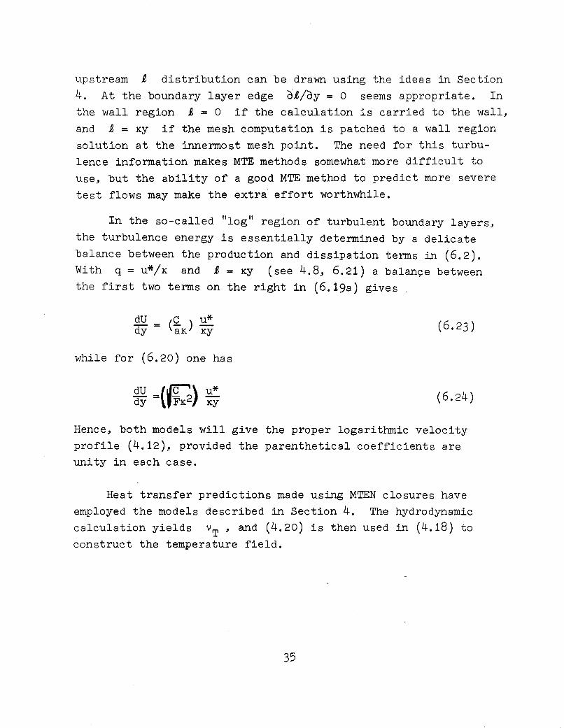
upstream £ distribution can be drawn using the ideas in Section4. At the boundary layer edge ~£/oy = 0 seems appropriate. Inthe wall region £ = 0 if the calculation is carried to the wall,and £ = Ky if the mesh computation is patche.d to a wall regionsolution at the innermost mesh point. The need for this turbulence information makes MTE methods somewhat more difficult touse, but the ability of a good MTE method to predict more severetest flows may make the extra effort worthwhile.
In the so-called "log" region of turbulent boundary layers,the turbulence energy is essentially determined by a delicate
balance between the production and dissipation terms in (6.2).With q = U*/K and £ = Ky (see 4.8, 6.21) a balange betweenthe first two terms on the right in (6.19a) gives.
(6.23)
while for (6.20) one has
(6.24)
Hence, both models will give the proper logarithmic velocityprofile (4.12), provided the parenthetical coefficients areunity in each case.
Heat transfer predictions made using MTEN closures haveemployed the models described in Section 4. The hydrodynamiccalculation yields vT ' and (4.20) is then used in (4.18) toconstruct the temperature field.
35

7. MTE Calculation Examples
The MTES approach has been advocated by Bradshaw and hiscoworkers (Bradshaw, Ferriss, and Atwell 1967, Bradshaw et al1966 et seq.). Their predictions for TBLPC must be judged amongthe very best. The agility of Bradshaw's MTES method to predictsevere flows was demonstrated at TBLPC by their results for theTillmann ledge flow, a boundary layer flow immediately downstreamof a turbulent reattachment point (judged the most difficultTBLPC flow). Fig. 15 shows their predictions at a point downstream in this flow, including results for two drastically different initial shear stress distributions. Note that the pre
dictions are very insensitive to the initial (upstream) shearstress distribution. In spite of the modest disparity betweenthe measured and predicted velocity profiles, the predicted
momentum thickness and skin friction were in considerably betteragreement with the data than were the MTEN and MVF predictions.Indeed, one left TBLPC with the feeling that Bradshaw and Ferriss'
MTES method was likely to be the wave of the future.
Nash (1970) has used a combination of Bradshaw's MTES ideasand a Newtonian assumption to treat three-dimensional turbulentboundary layers. Nash takes Bradshaw's structural assumption for
the total shear stress vector,
but then uses the Newtonian approximation
(7. 1 )
uv =uw
<lli&r.dW,7dZ (7. 2 )
which assumes alignment of the shear stress and strain ratevectors. The evidence is clear that (7.2) does not hold, yet itfortunately is worst in flows with strong spanwise pressure
I']

gradients, where the pressure gradients and n.ot the shear stresscontrol the mean velocity field. In Fig. 8 we show Wheeler andJohnston's (unpublished) calculation for the boundary layer alonga plane of symmetry approaching an obstacle. .The integral parameter predictions by MH's MVFN method, Nash's MTES/N method, andBradshaw's MTES method are almost identical. Nash's (1970) owncalculation for a point off of the symmetry plane in a similarflow is shown in Fig. 16. Mellor (1968) made a similar calculation with his MVFN method with comparable results.
Bradshaw (TBLPC-1) himself extended his MTES method tothree-dimension boundary layers, using the basic ideas to proposemodel equations for the vector sum and ratios of the two primarystresses, -uv and -wv. Johnston (1970) has compared theresult of predictions by this method with his own data for aninfinite swept flow. In particular, data show that the stressvector does not align with the strain-rate vector as the Newtonianclosures assume. Hopefully Bradshaw's structural model would workbetter on this flow but Johnston's calculation shows that theangle of the shear stress vector is predicted quite poorly,although the mean velocity is predicted quite well. It is unlikelythat MTE methods will ever predict this structural difference well,and one might hope that MRS methods will do considerably better.
Mc Donald and his associates (unpublished) have developed aMTES method following the lines of their integral method (TBLPC-1),and are using this method in a variety of boundary layer flows.They are also treating boundary layers using the full equationsin ord~r to study boundary layers near separation.
There has been considerable activity with MTEN computations.Beckwith and Bushnell (TBLPC-1) presented partial results fromtheir MTEN method at TBLFC, and have since continued with itsdevelopment. Spalding and his associates pushed ahead with MTES
37

program development. MH have added to the theoretical frameworkthrough their application of the method of matched expansions tothe selection of the length scale distribution functions, and byshowing how the MTEN equations arise as a limiting case of MRSequations for nearly isotropic turbulence.
The ability of MTEN calculations to accurately predict themean velocity field and turbulence kinetic energy distribution isdemonstrated by Figs. 17 from MH's TBLPC contribution. Their useof a fine computational mesh near the wall is reflected in theiraccurate prediction of the inner regions.
The MH MTEN predictions at TBLPC were among the best; weagain note that these predictions were identical with those oftheir MVF method for all but one TBLPC flow. Hence, for flowsnot too rapidly shocked by changes in free-stream or wall conditions, consi~tent MVF and MTE treatments may be expected to yieldnearly the same results for the mean velocity and integralparameters. Of course, only the MTE calculation yields theturbuler.~e energy distribution directly. Fig. 18 shows a MH MTENcalculation for a boundary layer responding to a sudden removalof adverse pressure gradient. Five years ago this would havebeen regarded as a "difficult" test flow, but we see that MTENmethods now handle it reasonably well.
The ability of MTEN methods to handle sudden changes inboundary conditions is evidenced by recent (unpublished) calculations QY Kays and his coworkers (see Loyd, Moffat, and Kays 1970 ).They have modified an early Spalding MTEN program to the pointwhere it successfully predicts the heat transfer behavior ofincompressible turbulent boundary layers with strong pressuregradients and with wall suction or blowing. With sudden changesin pressure gradient or blowing the heat transfer coefficient(Stanton number) changes rapidly, and such calculations are more
difficult for ~ methods.

For boundary layers the pressure gradient is convenientlyrepresented by the parameter
v dUooK =;::;;r - (7.3)u. dx
00
Fig. 19 shows a prediction by Kays (unpublished) of the heat
transfer to a boundary layer undergoing strong accelerationfollowed by a relaxation to zero pressure gradient. Note that the
sudden jump in Stanton number as the acceleration is removed ispredicted quite well. Fig. 20 shows another Kays calculation foran accelerated boundary layer, with blowing beginning midwaythrough the accelerated region and continuing through the relaxation to zero pressure gradient. Fig. 21 shows a prediction foran accelerated boundary layer with blowing, with transpiration
terminated upstream of the removal of acceleration. The remarkable success of these calculations suggests that MTEN methodsare now developed to the point of utility as tools for engineering analysis.
The MTE methods include a calculation of the turbulenceenergy, and hence one may study the effects of variable free
stream turbulence. Kearney, et.al. (1970) have compared suchpredictions with their data, and Fig. 22 shows a typical resultfor strongly accelerated turbulent boundary layer.
The MTEN methods have been applied to free shear flows to alimited degree by Spalding and his coworkers. Fig. 23 showspredictions by Rodi and Spalding (1970) for the asymptotic planejet. This calculation was made using their model equation for
the turbulence'length scale. Gosman et al (1969) have documentedthe Spalding MTEN program in detail, and advocate its applicationto heat and mass transfer in recirculating flows. Readers shouldbe aware that such programs are under continual development,which should not prevent their use in engineering analysis.
39

8. MRS Closures
In order to compute the structure or the turbulence (i.e.the Rij ), one must employ the dynamical equations ror the Rij(6.1). This has been the subject or considerable recent interest,though only a rew computational experiments have been carried outand a truly "universal" general theory has yet to be established.We can expect considerable activity on this rront, and review thecurrent status here with this in mind.
The problem is again to set up a satisractory closurestructure ror the unknown terms in the dynamical equations, herethe equations ror Rij . Some variation in approach is already
evident, and we may expect some interesting debate·on the choicesover the next several years.
Examination or (6.1) shows that the Rij equations containa pressure-strain-rate correlation term that vanishes in thecontraction (6.2). The errect or this term must thererore be totransr~r energy conservatively between the three componentsR11 , R22 , and R
33, and it is generally believed that this
transrer tends to produce isotropy in the turbulent motions.Modelings or this term should incorporate this feature. Aplausible model or this term (Rotta 1951), supported somewhat by
the data or Champagne, Harris, and Corrsin (1970) is,
dUo du.= *(ax~ + ~) =
J J.
2C ..9. (.9.....
35.. - R.. )
.f J.J J.J(8.1)
An objection to this model rests on the observation that the
fluctuating pressure rield is given by a Poisson equation,
d2= a a [u.u.-u.u.-u.u.-u .u.]x j x j J. J J. J J. JJ J.
40
(8.2)

This suggests that the P.. model should contain terms arlslngl.J
from interactions between the mean and fluctuating velocities,and should somehow reflect the dependence of the pressure fluctuations on distant velocity fluctuations. Daly and Harlow(1970, hereafter referred to as DH) have attempted to includethese effects in a complex closure approximation still in anexperimental stage (see 9.8a). Other MRS closure calculationshave all used (8.1). Some new suggestions are explored in
Section 9.
The pressure-velocity terms have been modeled in all MRScomputations of which I am aware by extensions of the gradientdiffusion model (6.8). Donaldson and Rosenbaum (1968, hereafter
referred to as DR) use
1 ORik- pu. = - q£ ~p l ~ oXk
DH use a similar expression with a more complex coefficient. MH
suggest
1- 1 0 2.- pu. = - - q£ ~p l 3 P xi
(8.4 )
Various forms of gradient diffusion models have been suggested for the triple velocity term. DR use and MH accept
(8.5)
The DH representation may be cast as
(8.6)
41

If the objections to a gradient-diffusion approach are valid,one should presumably use an extension of (6.9). A possiblelarge-eddy transport model is
The viscous terms have also been handled in different ways.DR and DH use Vij in the form (6.3). Following Glushko (1965),DR take
(8.8)
(8.9)
DH put
2DDij = q2 Rij
and use another differential equation for D. Dii =~/2v. MH,invoking arguments of local isotropy and using kinetic theory asa guide, propose using (6.S) with
(8.10)..-
and
(8.11 )
In order to complete the closure, the various length scales
in the models above must be prescribed or related to the otherindependent variables through a differential equation. DH use adynamical equation for i} , derived exactly from the NavierStokes equations and then closed by assumptions. The ~ equationwill be discussed shortly. DH are now considering the use of two
42
length scale equations for the dissipating and energy containingeddies.
MH have given considerable thought to the MRS closure, andshow how the MTEN equations emerge from MRS equations if it isassumed that the turbulence structure is nearly isotropic.
Calculations with MRS closure models have been carried outby DR, DH, and Harlow and Romero (1969). Harlow and Romero usedthe model with moderate success to study the distortion of isotropic turbulent (see Section 9). DR considered plane turbulentboundary layer flow in zero pressure gradient, and specifiedwhat seem to be reasonable length scale distributions for thiscalculation. DR's prediction of the mean veloc'ity profile isgood (but not better than a good MVF or MTE calculation); theirpredicted turbulent stress distributions, shown in Fig. 24 are insubstantial agreement with experiments. DH studied planePoiseuille flow with a more complex model, obtaining less satisfactory results. The DH model is not accurate near the wall, andis currently undergoing further extension and adjustment. Hirt(1969) gives a useful summary of the thinking behind developmentsin the Los Alamos group.
Thetheby
Let's now consider the IIdissipation ll transport equation.dynamical equation for ~ is derived by differentiatingmomentum'equation for ui with respect to x j '_ multiplying2vou./ox. and averaging. The result is
1 J
2 2}o ou. op 0 u. 0 u ..... dX:" (dJf.. dX":") + v (ax ~x. ax a~. )
j 11k 1 k 1(8.12)
Now, to obtain closure one must propose models of all the termsbetween the braces on the right hand side of (8.1 2 ). Thisrequires a considerable amount of courage as well as insight;there is no direct experimental evidence about any of the terms,and one can really only conjecture as to their effect. Lumley(1970) has used some rational reasoning for the special case of
homogepeous flows (~ection 9). DH used some qualitative ideasabout the effect of each term and proposed a model of (8.12), viz.
(8.13)
Here b1 and b2 are "universal parameters, all with values
near unity (or possibly equal to zero)", and F is.a function
44

of the turbulence Reynolds number. DH also in effect make the<>
assumption that iJ = e through their treatment of the R..J.J.
equation.
Hanjalic, Jones, and Launder (1970) propose a model of(8.12) which can be generalized as
0/7 + u 018 =ot jdX:"J
(8.14)
Here c1 and c2 are constants, and f 1 , f 2 ' and f3
arefunctions of the turbulence Reynolds number. They report that"encouraging" results are obtained when this equation is used
in an MTEN computational scheme. Clearly the use of such equations is presently quite experimental, and (8.14) is given hereto illustrate the rather substantial differences in ideas as tohow best to model (8.12).
For the special case of homogeneous flows at high turbulenceReynolds numbers (8.13) and (8.14) do have a common form. Bothmay be written as
011 + u 017 _ C ~2
+ C /)dJ"o:t jdX:"-- 12 22
J q q(8.15 )
where P is the rate of production of turbulence energy. Thisform is probably quite adequate for homogeneous flows (Section 9).
Lumley (1970) has studied the distortion of homogeneousturbulence by uniform strain using a limited MRS closure. Inhomogeneous flow the R.. equations become
J.J
45

dRi · ~Uj oU. 1 op Op~ = - Rik x
k- R
J'k d~l - - (u. ~ + u. ~)
K P J OXi 1 OX j
Lumley closes by taking
ou. ou. 51.' jV 1 -.:..:.J.. _ e
dXk 0Xk - 3
1 (u. ~ + u, ~)P J ~ 1 ox~
1 J
1 2 5 ..= (q -ll R )T 3 - ij
(8.16).
(8.17)
(8.18)
where T is a time scale of the turbulence (compare 8.1). Hefurther assumes that the time scale is related to th€ dissipationrate by
which is equivalent to (6.6). The dissipation rate is in turndescribed by
de e 2dt = - 4 2" (8.20)
q
as deduced by Lumley from scaling arguments-based on (8.12)
(compare 8.15).
Lumley has solved the equation system for homogeneous shear,and compared the results with homogeneous strain and homogeneous
shear experiments. Lumley's model predicts that the time scale Tgrows without bound, so that homogeneous flows can never attainan eguilibrium structure. Champagne, Harris, and Corrsin's (1970 )
46

experiments are consistent with Lumley's notion, but Lumley's
model does not predict the observed structure very well. Someimprovements on L~ley's model based on (8.15) are suggested inSection 9.
It does seem clear that equilibrium is never obtained inhomogeneous flows. In inhomogeneous flows the transport featuresapparently act to set the equilibrium structure. MTES methods
really shouldn't work in homogeneous flows, and we might well besuspicious of methods when the "universal constants" are obtainedby tests against such flows.
47

9. Some New Ideas for Homogeneous Flows/
It became apparent in preparing this review that too littleattention has been given to systematic development of theclosure model. The approach has been to construct a comprehen
sive model, with numerous universal constants, and then to selectthese constants by optimizing the average fit to a number ofselected flows. A more systematic approach would be to developthe closure model in a step-by-step approach, working gradually
through a heirarchy of experimental flows.
In order to develop some feeling for what might be accomplished, I examined the following approximations to homogeneousflow:
(1) Decay of isotropic turbulence (Townsend 1956)
(2) Return to isotropy in the absence of strain orshear (Tucker and Reynolds 1968, hereafter
referred to as TR)
(3) Development of structure under pure strain (TR)
(4) Development of structure under pure· shear(Champagne, Harris, and Corrsin 1970, hereafter
referred to as CHC).
The starting point of this analysis was the dynamical
for the turbulent kinetic energy and the dissipation.geneous flows these equations are
equations
For homo-
dq2;2dt = ~ - €
48

Here ~ = -RiJSij is the rate of turbulence energy production.Equation (9.1) is exact, and (9.2) is the form in which the dissipation equations of DH, Hanjalic, Jones and Launder (1970), andthe length scale equation of Ng and Spalding (1970) can beexpressed (see 8.15). For very weakly strained flows, Lumley(1970) developed the C1 term with C1 = 4 from first princi~
ples, and neglected the C2 terms in his weak strain model (8.20).Hanjalic et al suggest C1 = 4 and C2 = 3.2. Ng and Spalding's
empirical flow fitting is equivalent to C1 = 3.9 and C2 = 3.3 .
DH use C1 = 4 and C2 = 2 •
If one considers the decay of homogeneous isotropic turbulence with zero strain for large turbulence Reynolds numbers, andmodels the dissipation by
(9.1) and (9.2) produce
(9.4)
2 -1Now, experiments indicate that q V'\ t , it vo t which requires
C1 = 4. This seems a clear choice.
To investigate C2 I calculated the distribution of rP from
the data of CHC, and carefully determined an initial value for E
from the experimental q2 distribution (taking the starting pointat x = 5 ft in their experiments). The differential equations
49

(9.1) and (9.2) were then solved numerically for different valuesof C2 ; C2 = 2 is clearly preferred (Fig. 25a,b). A similarcalculation was carried out for the TR flow (Fig. 268), whereC2 = 2 also gives excellent agreement. Note that the predic~ed
length scale variations model the integral scale changes asmeasured by CRe (Fig 25b). It therefore appears that a satisfactory model equation for the dissipation history in homogeneous
flows is
Next I considered the Rij equations with the objective ofobtaining a model that, with (9.11) and (9.6), correctly predictsthe measured Rij • Closure assumptions are required for thepressure strain and dissipation term. In all calculations I took(6.5) and (8.11) in (6.1), and hence wrote
where the pressure-strain term is
E. oU i ou.Pij = (~ + ~)
p oXj 0XiI first took
(9.7a)
(9. 7b)
The first test was for the strain-free portion of the TR flow,where the structure is relaxing towards isotropy. Calculationsshowed that C
3= 5 gives a good representation of the structure,
energy, and production in this flow (Fig. 26b).
50

I then proceded to try (9.8) with C3
= 5 in the strainingregions o~ the TR and CHC ~lows, but was not satis~ied with theenergy predictions (see Figs. 25c,d,26c,d). It appears thatsome alteration in either the Pij or dissipation terms isrequired, and I chose to experiment with modi~ications in thePij . A ground rule was that proposed modi~ication could notalter what has already been systematically established. The~orms investigated were
P ..l.J
1 R. . 2= 5e (-3 5iJ· - l.~) + C4q s ..
q l.J
5 ( 1 5 _ R~j)= e '3 ij.q
(9. 9b)
Note that Pii = 0 in each case. Eq. (9.9a) is DH1s form withslightJ.,y di~ferent constants. Equations (9.9b)-{9.9d) aresuggested by the notion that interactions between the mean strainrate and fluctuation ~ields contribute to the pressure ~luctua
tions. The closures (9.9a) and (9.9b) were unsatis~actory. Forthe TR ~low (9.9c) with C4 = 1/2 works very well (Fig. 26c,d),but it is not adequate ~or the CHC flow (Fig. 25c,d). Equation(9.9d) reduces to (9.9c) ~or irrotational mean ~low, i.e. the TR~low, and with C4 = 1/2 and C5 = 1/4 (9.9d) predicts the CHC~low reasonably well (Fig. 25c,d).
51

It does seem clear that (9.7) is not adequate in flows withstrain or shear. With the constants indicated, (9.9d) is
1 Ri . 1 2Pij = 5€ (3 0ij - 7") + 2(Ri kSkj + RjkSki + 36>°ij)
+. 1 aU . aUk aU. aUk
4" [Rik(dt- - dX:") + RJ·k(aX~ - ~x,)] (9.10). k J . k J
which is probably better. Further development is needed, and(9.10) is offered here as an interim model. However, it is notclear that (9.10) is a model of Pij ; it could just as well be amodel for its complement (see 8.18) as used by Lumley (1970) in(8.16)!
52

10. Outlook for the Future
It should not be long before simple boundary layer flows
are routinely handled in industry by MVF prediction methods.
These methods are easy to use, require a minimum of input data,
and give results which are usually adequate for engineering
purposes. MTE methods will become increasingly important to both
engineers and scientists, for they afford the possibility of
including at least some important effects missed by MFV methods.The debate over the gradient-diffusion vs. large-eddy-transportclosures will continue, and both methods will probably continue
to be used with nearly equal success. MRS methods will beexplored from the scientific side, and porbably will not be used
to any substantial degree in engineering work for some time to
come.
Considerable effort is likely to be expended on the develop
ment of length scale (or equivalent) equations, such as thedissipation equation discussed in Section 8. In this connection
the two-point correlation
~ .. = u. (x)u .(x + ~)lJ 1 J
(10.1)
could be used to advantage, either along the lines of Gawain and
Pritchard (1970), or perhaps through a closure of its own
dynamical equation (Hinze 1959).
This equation will of course involve six independent space
variables, but by integration over the separations ~ thesevariables could be removed. Then, one might assume the form of
Rij , say
~ ..lJ
53
(10.2)

and carry out the integrations, thereby obtaining three additional differential equations of the transport type relatingthe integral scales £i and the one-point correlations(turbulent stresses) Rij . Experimental calculations alongthese lines would be most interesting.
The heavy computation approach (Deardorff 1970) might beused to numerically test the closure assumptions used in the
simpler MRS and MTE models. Hopefully such computations will bedocumented in the future with this use in mind.
The MRS closures will attract most interest for use whereMTE methods fail. For example, in flows with rotation thecoriolis terms enter the Rij equations, but drop out in theequation for R.. = q2. Therefore, it probably will be
II
essential to go to a MRS method to include rotation effects, whichare of considerable importance in many practical engineering andgeophysical problems. Other effects which have not yet beenadequately modeled and for which MRS methods may offer some hopeinclude additive drag reduction, ultra-high Reynolds numb~rs,
separation, roughness, lateral and transverse curvature, andstrong thermal processes that affect the hydrodynamic motions.
We might also see the complex closure models used as thebasis for computationally simpler integral methods. The successof integral'methods of this type at TBLPC (MC,HR; TBLPC-1) shouldnot be forgotten in the rush to use the full partial differential
equations.
A disappointing aspect of the current status is that very
little use has been made of the substantial advances made over thepast decade in our understanding of the structure of turbulentshear flows. We know that large eddy structures dominate such
flows; only MTES methods recognize this at all, and then not

quantitatively; MTEN methods ignore it all together. MRS calculations have not used the large eddy idea at all. Indeed, the
concept of a "transport theory" for turbulent correlations wouldseem antithetical to a large eddy view. We know that the wall
region is dominated by a particular correlatable structure, yetnone of the current prediction methods make any use of this fact.The structure of the outer region of boundary layers has been
extensively studied recently, and entrainment of non-turbulentfluid through the turbulent interface (superlayer) is known tobe a critical process in turbulent shear flows; no real utilization of this fact has been incorporated into any of the closuremodels. We know that the outer layer flow has a dual structure,intermittently consisting of turbulent and non-turbulent regions
with considerably different character. Yet all calculationmethods are based on averages taken over long periods of time,averages that wash out this essential feature of the flow. Somebelieve a similar duality exists in the wall region; might notthis also be incorporated?
In short, it seems that too much attention has been paid tothe numerical aspects of the computations; indeed, the difficultyof a first encounter with complex differencing schemes has madethis necessary. But now we should begin a concerted effortto bring the new physical information into the turbulent flowcomputation methods, and we look for a better situation ten years
hence.
Finally, for those who cannot or choose not to take up thecomputation game, perhaps some fresh thinking at the fundamentallevel might be fruitful. For example, we all want to computeturbulent flows. Just what is it that we are working so hard tocompute? What is the operational definition of turbulence?
55

REFERENCES
Bradshaw, P. et al 1956 et seq, Calculation of boundary-layer
development using the turbulent energy equation, Natl.Phys.
Lab. Aero Div. reports 1182, 1217, 1271, 1286, 1287, 1288
Bradshaw, P., Ferriss} D. H., and Atwell, N. P., 1967 Calculations
of boundary layer development using the turbulent energyequation, J. Fluid. Mech., 28, 593
Bradshaw, P., 1970 The use of transport equations for Reynoldsstress (to appear).
Busse, F. H., 1970 Bounds for turbulent shear flow, J. Fluid.Mech., 41, 219
Byrne, J. E., and Hatton, A. P., 1970 Prediction and measurement
of velocity and temperature profiles in turbulent boundarylayers
Cebeci, T., Smith, A.M.O., and Mosinskis, G., 1969 Calculation ofcompressible adiabatic turbulent boundary layers, AIAA paper
69-687
Cebeci, T., 1970a Application of exact turbulent boundary layerequations as a means of calculating heat and mass transferin incompressible and compressible flows, Preprints, Fourth
International Heat Transfer Conference, Paris.
Cebeci, T.,.1970b A model for eddy-conductivity and turbulentPrandtl number, Report MDC-j0747/01, McDonnell Douglas Co.
Champagne, F.H., Harris, V.G., and Corrsin, S., 1970 Experimentson nearly homogeneous turbulent shear flow, J. Fluid. Mech.,
~' p 81
Daly, B.J., and Harlow F.H. 1970 Los Alamos Scientific Lab preprint LA-DC~11304 (to appear in Phys. Fluids)
Davis, R.E., 1970 On the turbulent flow over a wavy ~oundary,
J. Fluid Mech. 42, 721
56

Deardorff, J.W., 1970 A numerical study of three-dimensional
turbulent channel flow at large Reynolds numbers, J. FluidMech... 41, 453
Donaldson, C.D., and Rosenbaum, H., 1968 Calculation of turbulentshear flows through closure of the Reynolds equations byinvariant modeling, Aero Res. Assoc. of Princeton Report 127
Gawain, T.H., and Pritchard, J.W., 1970 A unified Hueristic modelof turbulence, J. Compo Physics., 5, 385
Glushko, G.S., 1965 Turbulent boundary layer on a flat plate inan incompressible fluid, NASA TTF-10,080 (translation ofIzv. Akad. Nauk SSSR (Mekhanika), 4, p 13
Gosman, A.D., Pun, W.M., Runchal, A.K., Spalding, D.B., andWolfshtein, M., 1969 Heat and mass transfer in recirculatingflows, Academic Press, London
Hanjalic, K., Jones, W.P., and Launder, B.E., 1970 Some notes onan energy-dissipation model of turbulence, Imperial Col.,London (internal report)
Harlow, F.H., and Nakayama, P.I., 1967 Turbulence transportequations, Phys. Fluids 10, 2323
Harlow, F.H., and Romero, N.C., 1969 Turbulence distortion in anonuniform tunnel, Los Alamos Lab report LA-4247
Harlow, F.H., and Nakayama, P.I., 1969 Los Alamos Scientific Lab
preprint LA-DC-8635
Herring, H.J., and Mellor, G.L., 1968 A method of calculatingcompressible turbulent boundary layers, NASA CR-1444
Hinze, J.O., 1959 Turbulence, McGraw Hill Book Co., Inc.
Hirt, C.W., 1969 Computer studies of time-dependent turbulent
flows, Phys. Fluids, ~,II-219
Howard, L.N., 1963 Heat transport by turbulent convection,
J. Fluid Mech., 11, 405
57

Hussain, A.K.M.F., and Reynolds, W.C., 1970 The mechanics ofperturbation wave in turbulent shear flow, Report FM-6,Mech. Engrg. Dept., Stanford. See also J. Fluid Mech., ~,241
Johnston, J.P., 1970 Measurements in a three-dimensional turbulentboundary layer induced by a swept, forward facing step,J. Fluid. Mech., 42, 823
Kasahara, A., 1969 Simulation of the earth's atmosphere, CompoApproaches in App. Mech., ASME
Kearney, D. et al 1970 The effect of free-stream turbulence onheat transfer to strongly accelerated turbulent boundarylayers, Proc. 1970 Heat Transfer and Fluid Mech. Institute,Stanford U. Press
Kendall, J.M., 1970 The "turbulent boundary layer over a wall withprogressive surface waves, J. Fluid Mech. 41,
Kline, S. J. et al 1967 The structure of turbulent boundary layers,J. Fluid Mech., 32,741
Lighthill, M. J., 1952, Reviews, J. Fluid Mech., !, 554
Loyd, R.J., Moffat, R.J., and Kays, W.M., 1970 The turbulentboundary layer on a porous plate; an experimental study ofthe fluid dynamics with strong favorable pressure gradientsand blowing, Report HMT-13, Mech. Engrg. Dept., Stanford U.
Lumley, J.L., 1970, Toward a turbulent constitutive equation,J. Fl~id Mech., 41, p. 413
Lundgren, T. S., 1967 Distribution functions in the statisticaltheory of turbulence, Phys. Fluids, 12, 969
Mellor, G. L., 1967 Incompressible turbulent boundary layers witharbitrary pressure gradients and divergent or convergent
cross flows, AIAA Jour., 5, 1570
Mellor, G.L., and Herring, H.J., 1970a,b, A study of turbulentboundary layer models (a) Part I, (b) Part II, ,Sandia Lab.
Report SC-CR-70-6125.
58

,Nash, J.F., 1970 The calculation of three-dimensional turbulentboundary layers in incompressible flow, J.Fluid Mech.,31, 625
Ng, K.H., and Spalding, D.B., Some applications of a model ofturbulence for boundary layers near walls (to appear inPhys. Fluids--see also Imperial Col. report B1/TN/14,Aug. 1969)
Patankar, S.V., and Spalding, D.S., 1967 Heat and Mass Transferin Boundary Layers, C.R.C. press, Cleveland. See also Int.J. Heat and Mass Trans., 10, 1389
Prandtl, L. 1945 Nach. Akad. Wiss. Gottengem, Math-pysile, K. 1(liOn a new representation of fully developed turbulence",
JPL Publication No. 13 (1952), trans. by. D. Coles)
Rotta, J.C., 1951 Zeitschrift fur Physik, I: 129,547-752; II:
ill, 51-77
Russell, B., 1961, A History of Western Philosophy, Allen andUnwin, London
Simpson, R.L., Whitten, D.G., and Moffat, R.J., 1970 An experimental study of the turbulent Prandtl number of air withinjection and suction, Int. J. Heat Mass Trans., 12, 125
Spalding, D.B., and Rodi, 1970 A two-parameter model of turbulenceand its application to free jets, Warme-und StuffUbertragung,
.3., 85·
Stewart, R.H., 1970 Laboratory studies of the velocity field overdeep water waves, J. Fluid Mech., 42, 733
TBLPC 1968 Proceedings - Computation of Turbulent Boundary Layers1968 AFOSR-IFP - Stanford Conference; Vol. 1 (Ed. K~ine et al)Methods, predictions, evaluation and flow structure; Vol. 2(Ed. Coles and Hirst) Compiled data; Thermosciences Div.,Dept. of Mech. Engrg., Stanford U., Stanford, Ca. 94305.
59

Townsend, A.A., 1956 The structure of turbulent shear flow,Cambridge U. Press
Tucker, H.J., and Reynolds, A.J., 1968 The distortion of turbulence by irrotational plain strain, J. Fluid Mech. ~' 657
60
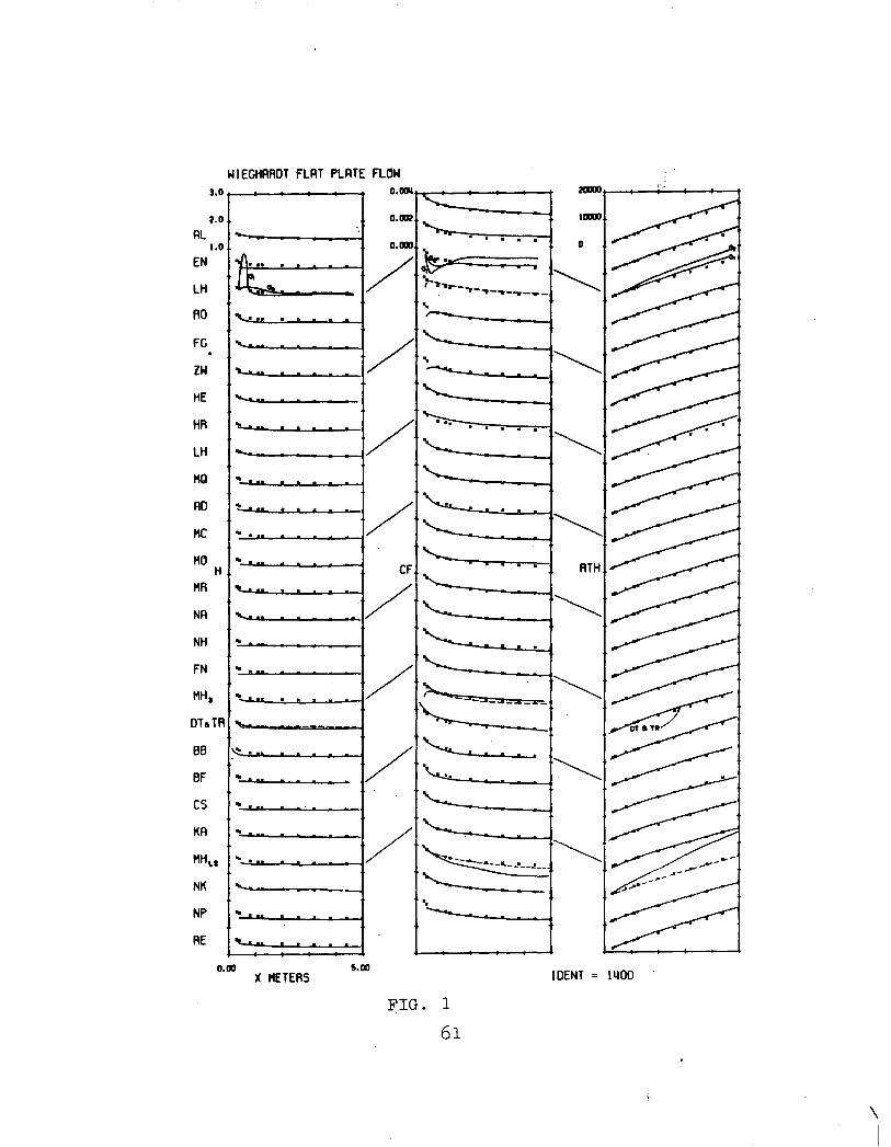
WIEGHRAOT FLRT PLRTE FLOW
NK .....................---..--.----..J
KA '"'-&.0'_..--..1...... 1
HHu ...-:.....- .......--"'-.&--4
. r,.
. .
· . .
-- « ..
'-' ..
'.0 t-"-----------t
BB ~_'" ' "--L.-IL..-&........__I
BF ...."""., ---'........ _
CS
NP ...-oLM.--'......................... 4
RE
:l.0
AL ...1.0
EN ..{\... ·LH LL.RD
..... ·FG
ZW .......HE ...........
HR .......LH ~
HQ ~ ..AD ...
HC '" .HO ...
HHR 'lL.
NA ......
NH ...
FN ...
HH I ~ ... · . .OT.TR .....
0.00X METERS
5.00 IOENT 1400
FIG. 1
61
\
I

llOlIllDr--~- .
----,,~..
•
O.aoo
..
0.001
."
I•/,/
_....-_ 1_____ \_.-'-1
'\... .-------~----~~ .. :.~
"'"'---"- .
...... .
~ ~~ ';-
-----~--- /e----.-, ~ .'?:~
", - '- . .---- .
.~CF~ /RTH r ~
----- ~--- / ./DT~_----J----- ~---
-'''.'': \ . .,,"';--&._-
...---.
./
BRADSHAW A = -0.255o.lJ02r-- ~.
NP
RE
HR
NA
HH,.•
NK
Z.O
AL1.0
EN
LH
RO
FG
lW
HE -HR
NH
FN
LH
HC
AD
HC
HOH
MH.
DT.TR
BB
BF
CS
KA
\.00 X FEET 7.00 IOENT = 2600
FIG. 2

I INTEGRAL METHOD
25 P PARTIAL D. E.p+ TURBULENCE .P. D.E.. I
I
20 I II I
IP
15 Im I
>-10I
Ial I(!) Iz 5 p+P- I ~RP+to-« I 'Q: I
p+
C:>~ 5 10 15 20 25'~
RATING BY A<c
FIG. 3
63

It)
r--,.--..,...-r---,~r--..,..~....JgI
~
AI ~ 0_ "~O d
· 0 : I0-
It)odI
C\IooI .
+.0..
-od
I
o
-o~_--'__"""'_-I-J....jL-..JL......l.llJU dgoo 0 0 0+
ex> <D ~ C\I
+<{
64
.dHJ3:i

0,18 - - -
o yNOT TO SCALE
FIG. 5

...LaJ-,:)
(/)..J
... ..Jz <t
(!) c ~z ...- (/)(/) z::) 0
(,)
z0- c... ... IC
U CG '0
- 0 I·0 ::J
.LIJ M
Cl
It: "-H~
a.. ::J
..... -J._......__..--.--'0~ 0
66

It)•o
o
I-'ZUJ-0<t 00::
8~C)z =>°UJ ..... t--0::0:: => .I-=> 0
HWC/) Ii.
<tC/)UJ
zO::0-n..
I-lLJUJc/)-")0::...JL&J...J><to~<t
0It) U)
It)0..
CD 0- .s::.. u>- c
67

q-.o
~IN,0 --0
....-.-:lI
8 8L-d-90°
N•o
z.......Z en enu. LLJ LLJ> t- t:E 2·:e
IIII
NOlLYHYdi S
68
(J)enCD
.s:=oc
..x

O. .- CD,.... .- ,....~U
vQ)
~
tf)
~(J"I.
N dII H
(]) p:.
a:
-+-.....- .........- .....---ll--....-+---+-.....--+OU>. V. C'i 0
69

x
00 It) Q II') 0 0 a ONN a d ~ ~ 0. O.d 0 0 0-a>~
0ID
<XlNII
82
c:
~-=0')10
i r
70

RS
-=5
50
0at
X=
24
.0--
JI-
'
M=
2.8
0.6
0.4
U.U U
.F
IG.
lOb

o
X, fto
0.0004
0.004
0 0
hi'
NASA TN-O 1743RUN 2
Ibm 0.002
RAO NOZZLE
sec - in20.001
0
FIG. 11
72

>-a::<t00::zw::>>o<tCD....J
73
eltelo<1
>r-->«u
.ClH~

.ClHrr..
o..
>-.uzw::).... a
'3 "'w.-Q) a:
z LL0-....... en0- -enC wLaJ
<t....J
a:: zCL. t- o,c <t In-
C ·enZ OzLL IJJ> ::E:i -c
~38~nN 3A"VM SS31NOISN3WIO
74

.D
C'C.:::tM
CI)
d.......... HcU .D II.<
"--' .......,
N-<3-It) 0N-
0
0
'"0...
I0
'"II 0
I '"I 0-- -I '0
.Q I I ~IE 0
'"Go 0
It) 0 0 0 0 0 0 ~
~ 0 0 0 0 0 0N ", It) ~ 0
0
~
N
75
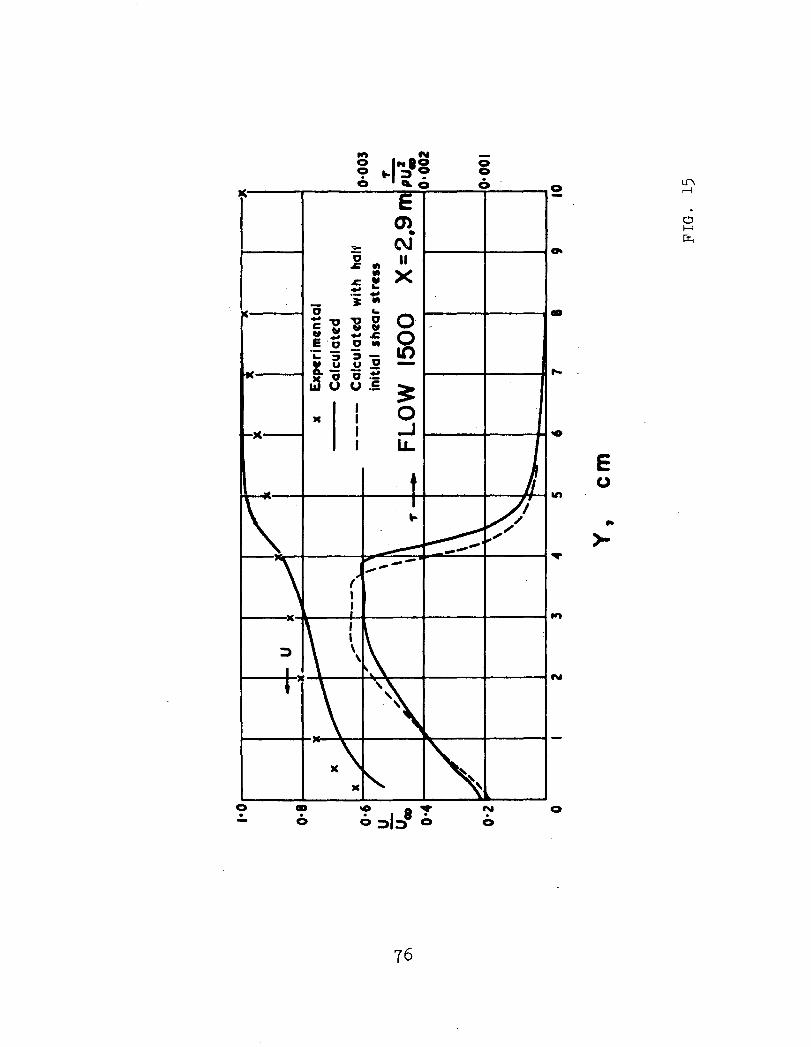
0·00
3
0'00
1"- PUz •
0·00
2
'09
87
65
..3
2
~~
l~
-~Ux~
x
~~
xE
xpe
rim
en
tal
)(C
alcu
la·te
dx
/,.
--~--
....----
Calculat~
wit
hh
alf
,----
//V
\'
init
ial
she
ar
stre
ss
/'
\
\\
FLO
W15
00X
=2
.9m
\'f
'-~
V\\
I
'\~~
......
1·0 o
0·8
0'2
0'6
Y...
U.
0'4
--J
0\
Y,
em
FIG
.15

-CD 8·0:),
\..0:) --1
CO .· d
0 HIi<
•·0
•C'!:)0,
~
0- 0fit) C\I-- .)-c.-\ ,
\
77

o~
0rt)
0.j........
. 'If. 0 O' <1 f:P ~
::>.......
....... c *::>
~0
:::>>-
QN
o-
0
0 It) 0- *~
::::> ::::>....... .......::::> r:P
78
. \
' .. ~
.CJH~

r') .0
• r---
0;-1
.dHrr,
Ct-eE0 C\I·<J 0
•o
0
0
" -.!"0
:::)
I ~.......
8 :> cO:::)
79

5.0
4.0
Ctn~ a...... ~V(\JII -
)( ">
rt)~-
0'10~-
..... 0 rt)0(X)- If) 0
0'1
3.0y (in)
2.0
1.0
1.0 0.5 1.0
U/U GO
5.0
4.0
3.0y (inl
. 2.0
1.0
QOO4 QOO4 . 0.004 0.004 . QOO4
LlpU~
0004 0004
5.0
••
H°0"-~;;"";"-+--~':""':"_"""--'::"'--:::+-=-:=---_-4=-----"+-:-----'-;"';;'-'-
Q02 0.01 Q02 001 0.02 0.01 0.02 QOI Q02 QOI Q02 001 002
4.0
1.0
3.0y (in)
2.0
FIG. 18 80

·z.J o&&.1_u(,')U&&.I~a:
CDI0
I )(
0'1
en
,..-i
CD It)
.
0.
0
- (\J
H
en II
rr..
0~
z:::>a:
,.X
rt')
-
ort')
oo.o ....
en
(\J
oo.o
81
ooo
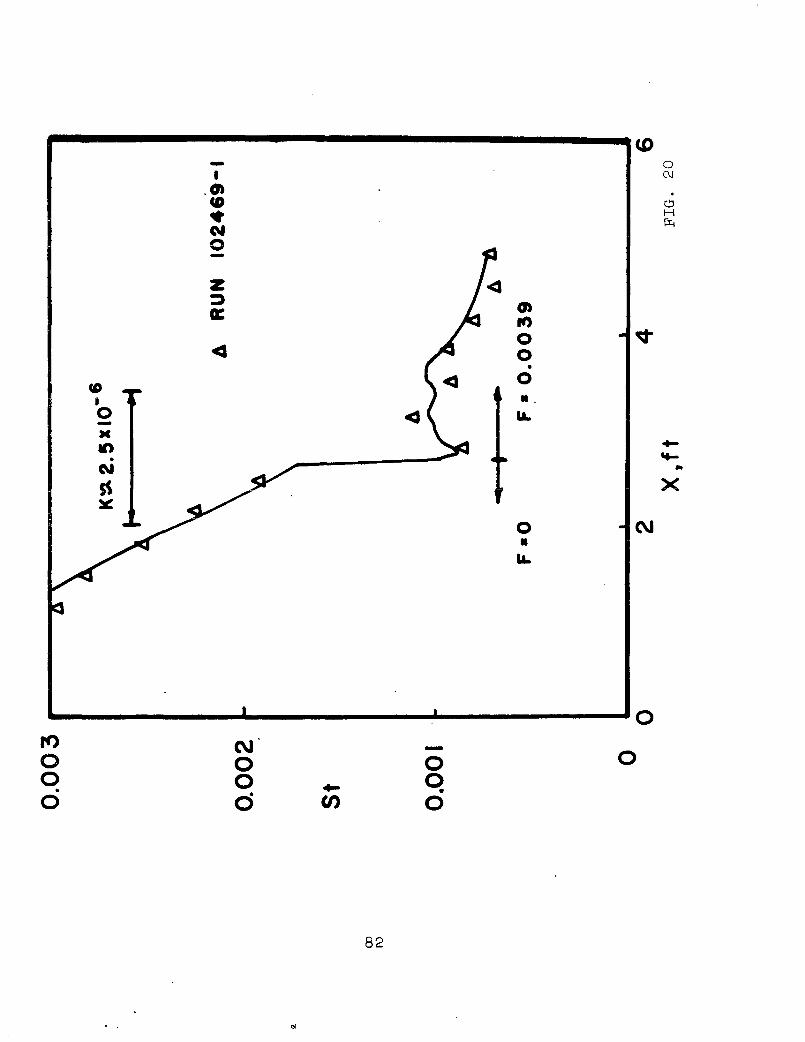
CD- 0I C\l
.~ .CD d~
Hfr.l
'"0-Z~ CJ'a: If)
0~ 0
•0
CQ •••0 ~ .....Ie ...It)
'to-.N ..~ X~
0 (\J
•.....
oo•o
-Nood
It)
oo.o
....-------1.------....---------0o
82

0.002
St
0.001
6 RUN 111369-2
F -0.004 F- 0• I •
o o I 2 :3X, ft
FIG. 21
83
4 5

C\JC\J
~'--"""E1+
cDIo
I!J+ %
CDa::
84

o
(Yl
-J
(\J
I
0
Z
H
IJJ
J:i:.<
t-~
t- Een::>z z
0 1LJ- ~.... -~
u a:- I.LJ
-0
to
1LI Q.
"a: x
>-a. I.LJ
I
-t- Iw IJ
IwZ<t
I~ E-J
:JQ.
0-~
I#
#leI :JI::>
00an
•-0
85

" MRS" ---- DATA
\\
\\
\~ ,
",~ ~
-uv xO.I/U..
0.1
o
o
0.08
0.04
0.06~ (U2fUm
" " "
o ....--....__a.-_-....__......._~o 0.2 0.4 0.6 0.8 1.0
Y/O
FIG. 24 86

FIGS. 25a, b
87

10\
"8
R··II
R .._~.L x .04
2 I 6Uo --- DATA( ..\ c )
RII4 "-R
22,- "- --,,,,- --..........,
R33
...........C
2 ~
-- --- RI2 B
02 x/h 6 10
0.8
--- FROM E CALCULATION
•In
0.4 ( d )
2 x/h 6 10
88 FIGS. 25c, d

INITIAL SLOPE FROM EXPONENTIAL
24 FIT TO TUCKER and REYNOLDS' FIG. 6
--- EXPERIMENT
8
4
Q.. in
o
(n)
3
8040X, in
6~--..J-----.L._--.l--_-""""'----~
o
0,6
0.4
:// / I DATA RANGE
8
7
j ,in
6
( b )
100 120X, in FIGS. 26a, b
89

24 -- - EXPERIMENT
18
12
( c )
6o 40 X, in 80
0.6
R33 - RII
R33 +Rll 0.4
(d) 0.2
FIGS. 26c, d
- -- ~ FROM €EQN.
/ 1// DATA RANGE
40 X,in 80
90
12
8
4