Digital Comprehensive Summaries of Uppsala Dissertationsfrom the Faculty of Science and Technology 23

Water and Heat Transport in Road Structures

KLAS HANSSON

Development of Mechanistic Models

ISSN 1651-6214ISBN 91-554-6172-7urn:nbn:se:uu:diva-4822

ACTAUNIVERSITATIS

UPSALIENSISUPPSALA

2005

ISBN

List of papers

The thesis contains references to the following appended papers, which in the comprehensive summary are referred to by their roman numerals:

I Hansson, K., Šim nek, J., Mizoguchi, M., Lundin, L.-C., van Ge-nuchten, M.Th., 2004. Water Flow and Heat Transport in Frozen Soil: Numerical Solution and Freeze/Thaw Applications. Vadose Zone J., 3(2):693-704.

II Hansson, K., Lundin, L.-C., Equifinality and sensitivity in freezing and thawing simulations of laboratory and in situ data. Cold Re-gions Sci. Tech., submitted 2004-02.

III Hansson, K., Lundin, L.-C., Šim nek, J., Modeling water flow patterns in flexible pavements. Presented at the 84th Annual Meet-ing of the Transportation Research Board, Washington, D.C., 2005, and accepted for publication in the 2005 series of the Transporta-tion Research Record: Journal of the Transportation Research Board.

IV Hansson, K., Lundin, L.-C., Water content reflectometers for coarse materials: Application to construction materials and effect of sampling volume. Submitted to Water Resour. Res., 2005-03.

The Soil Science Society of America (I), and The Transportation Research Board, The National Academies (III), kindly gave permission to reprint the indicated papers.

The author of this thesis was responsible for simulations, analysis and writ-ing in all papers. Jirka Šim nek developed the numerical scheme used in papers I and II, and implemented it in the HYDRUS codes. Jirka Šim nek also implemented surface runoff and particle visualisation in the HYDRUS-2D code (paper III).

Contents

1 Preface ...................................................................................................7

2 Introduction ...........................................................................................82.1 Background ..................................................................................82.2 Objectives.....................................................................................9

3 Fundamental concepts of porous media...............................................113.1 Potential theory...........................................................................113.2 Hydraulic properties ...................................................................12

3.2.1 Water characteristic equation.................................................133.2.2 Permeability and hydraulic conductivity ...............................143.2.3 Unsaturated hydraulic conductivity .......................................153.2.4 The effect of ice on hydraulic conductivity ...........................163.2.5 Prediction of soil hydraulic properties...................................17

3.3 Thermal properties .....................................................................193.3.1 Thermal conductivity.............................................................193.3.2 Heat capacity .........................................................................203.3.3 Thermal diffusivity ................................................................20

3.4 Freezing and thawing .................................................................203.4.1 The unresolved problem of freezing ......................................203.4.2 Miller-type models.................................................................213.4.3 Hydrodynamic models ...........................................................22

3.5 Measurements of water content in granular materials................233.5.1 A short review of methods to measure hydraulic properties .233.5.2 Measurements based on dielectric properties ........................24

3.6 Effects of water content variations on road damage...................25

4 Modelling approach .............................................................................274.1 Water flow..................................................................................274.2 Heat flux .....................................................................................294.3 Apparent volumetric heat capacity .............................................294.4 Thermal conductivity .................................................................314.5 Surface runoff.............................................................................324.6 Fracture zone water flow............................................................334.7 Numerical solutions to the water and heat transport equations ..34

4.7.1 What is a numerical solution, and what are the benefits of numerical methods? ..............................................................34

4.7.2 Meshes ...................................................................................354.7.3 Discretisation of the differential equation..............................37

5 Freezing simulation of a column experiment (paper I)........................415.1 A new freezing/thawing algorithm.............................................415.2 Validation of the numerical method ...........................................42

6 Uncertainty analysis of the freezing module of the numerical model (paper II)...............................................................................................44

7 Sensitivity of road design criteria to changes in operational hydrological parameters (paper II) .......................................................47

8 Effect of rainfall and fracture zone conductivity on the subsurface flow pattern (paper III) .................................................................................49

9 Application of TDR and WCR in road materials (paper IV)...............519.1 Dielectric models........................................................................519.2 A function yielding the dielectric number from WCR output....519.3 A numerical model to simulate the WCR response....................539.4 Evaluation of WCR calibration equations ..................................549.5 Simulation of the distortion in sampling volume .......................55

10 Conclusions .........................................................................................56

11 Future developments and recommendations........................................5711.1 Research phase ...........................................................................5711.2 Application phase .......................................................................58

12 Acknowledgements..............................................................................59

13 Summary in Swedish ...........................................................................61

14 References ...........................................................................................64

Abbreviations

FD Finite Difference FE Finite Element FV Finite Volume GLUE Generalized Likelihood Uncertainty Estimation NCED Normalized Cumulative Efficiency Distribution PDE Partial Differential Equation PTF Pedo-Transfer Function RMSE Root Mean Square Error SNRA Swedish National Road Administration (Vägverket) TDR Time Domain Reflectometry UHC Unsaturated Hydraulic Conductivity WCE Water Characteristic Equation WCR Water Content Reflectometry

7

1 Preface

The title of this thesis is “Water and heat transport in road structures - devel-opment of mechanistic models”. Connecting to the title, the introduction will explain which role water and temperature play in determining the degrada-tion of roads, and thus presenting some motives why this study was initiated by the Swedish National Road Administration (SNRA) about four and a half years ago. The original project name was “Water flow model”, which indi-cates that the overall objective was to develop a numerical model that could be used to predict how moisture in the road is redistributed due to relevant time-variable physical boundary conditions such as weather. Shortly, it will become evident that such an analysis benefits greatly by the inclusion of heat transport, and thus the thesis title differs from the original project name.

This thesis encompasses most of the relevant hydraulic and thermal proc-esses involved in describing the subsurface domain of a road, and in addition surface runoff. However, the important energy exchange processes at the asphalt surface are hardly mentioned at all, and for such a treatment, the author refers to the nearly completed PhD thesis works of Esben Almqvist at the Earth Sciences Centre at Göteborgs universitet, and of Christer Jansson at the Dept. of Land and Water Resources Engineering at KTH in Stock-holm. In addition, snow is not considered and is likely to play an important role for the hydrology of the road vicinity, in terms of thermal insulation of the road sides, snow melt percolation, and concurrent release of de-icing salt to the ground.

In order to make the contents of this thesis at least somewhat accessible to people with a general science or engineering background, some of the basic principles and ideas of the theory on which the thesis rely will be reviewed in chapter 3. The reader is advised to recall that this study was influenced by the perspective and theories of a soil physicist and hydrologist, and conse-quently the focus is on the pores between the particles rather than on the particles themselves, the latter being at the centre of attention in most geo-technical studies.

8

2 Introduction

2.1 BackgroundIn contrast to a statistical model, a mechanistic model comprises processes observed in reality. These processes act to change various state variables (such as temperature) as dictated by physical laws (equations). One of the premier, and first, advocates of a mechanistic view on the world was René Descartes who in Principia philosophiae {1644} describes an entirely mechanistic universe where the movement of everything is governed by the causal relationships of nature. A few decades later, the processes described by Descartes were expressed in form of equations by Isaac Newton in his famous work Philosophiae naturalis principia mathematica {1687} in which Newton e.g. presented his famous law on gravitation (cited by Eriksson and Frängsmyr, 1993). The works of Newton formed the basis for our definition of a mechanistic model (often called physically based model) – i.e. a set of equations that describe real, observable physical processes. This means that the model-processes, which attempt to mimic these real processes, contain parameters that are possible to measure (like the ability of the ground to conduct heat), and thus the model can ideally be applied with success in a variety of locations (e.g. all over Sweden) by changing the model setup to account for, in this case, different road structures, different climate, different underlying soil. A statistical model however, is only applicable for the loca-tion and road structure that it was calibrated for. With the advent of com-puters came numerical models, which allowed much more complicated and realistic mathematical problems to be solved. Since a numerical mechanistic model embodies processes, it can be used to investigate effects of changes in e.g. climate or construction.

Returning to the water and heat transport, these processes, which act to change or retain water content, ice content and temperature, have a direct impact on the lifespan of the road and consequently on the economy of the society as a whole. E.g., in 1994, 25% of the Swedish national roads were subjected to load restrictions; in northern Sweden as much as 40% of the road network may be inaccessible during spring thaw (Simonsen and Isacs-son, 1999); and during 2005 the Swedish government has allocated 1.22 billion SEK to freeze/thaw related improvements and reconstructions of roads already damaged (Näringsdepartementet, 2004). Diefenderfer et al.

9

(2001) listed some non-exclusive effects of excessive moisture in road struc-tures:

reduction of the shear strength of unbound subgrade and base/subbase materials, differential swelling in expansive subgrade soils, movement of unbound fines into flexible pavement base/subbase courses, frost heave and reduction of strength during thaw, pumping of fines and durability cracking in rigid pavements, and stripping of asphalt in flexible pavements.

No roads are built to last forever, and a common design life can be e.g. 50 years. The prediction of the life span of a road involves assumptions con-cerning the development of traffic volume, and the load that the traffic ex-poses the road structure to. Furthermore, the deterioration varies over the year since the material properties decisive for the resilience of the road de-pend on temperature (mostly asphalt) and water and ice content respectively (mostly unbound materials). In conclusion, in order to somewhat precisely predict the lifespan of a road, defined as the time from construction to fail-ure, appropriate values of temperature, water and ice contents are needed. Thus, future road design will include more computer simulations of the deg-radation processes described by mechanistic models using time-variable climatic boundary conditions.

Numerical models of heat and water transport are in addition useful when studying transport of dissolved substances in the road structure and in the ground on which the road rests. As an example, the author is currently in-volved in a project concerning guidelines for the use of waste material in road structures where simulations of leaching of solutes from the waste are one component of the study.

2.2 Objectives The intent of this study was to develop mechanistic models, and measure-ment techniques, suitable to describe and understand water flow and heat flux in road structures exposed to a cold climate. In the process of fulfilling the addressed purpose three more detailed objectives were identified:

1. To develop a numerical model that was suitable for cold climates, i.e. that included freezing and thawing algorithms. The model should also include processes essential for a two-dimensional description such as surface runoff.

10

2. To investigate the model response to variations in parameter values and demonstrate how the model can be used to address important practical problems related to freezing and thawing.

3. To evaluate the feasibility of water content reflectometers when working with coarse materials and find a suitable calibration equation.

11

3 Fundamental concepts of porous media

3.1 Potential theory Potential is a concept used in many branches of science to study dynamic processes where various properties such as energy, mass, or momentum are transported in a direction governed by the gradient of the potential and with a magnitude governed by one or more flow coefficients (e.g. Claesson, 1993; Fox and McDonald, 1994). In soil physics, the potential, , consists of sev-eral constituents as defined by

eaogw [1]

where w is the soil water potential, g is the gravitational potential, o is the osmotic potential, a is the pneumatic potential, and e is the envelope poten-tial (e.g. Kutilek and Nielsen 1994). The soil water potential is the result of e.g. capillary and adsorptive forces, and depends on the water content. The gravitational energy reflects what is called potential energy in mechanics, i.e. it is proportional to the work required to lift water from a certain reference height. Osmotic potential arises from differences in chemical composition for water at the same elevation. Pneumatic potential accounts for air pressure differences between the air inside the pores and the air outside of the soil, which is at atmospheric pressure. Finally, the envelope potential is a result of mechanical pressures such as the overburden pressure. In the context of roads this potential is affected by traffic loads and has been shown to gener-ate significant water flows beneath slabs in a concrete road in Florida (Han-sen et al., 1991). Still, it is often reasonable to reduce Eq. [1] to

gw . [2]

Furthermore, Eq. [2] may be expressed in the convenient head units [energy per unit weight of water = metre] by division with the density of water, ,and the gravitational acceleration, g, leading to

12

zhH , [3]

where the gravitational head, z [L], is the vertical distance from a reference level. Pressure head, h, is related to water content in a complicated way, which in turn depends on the elevation above the groundwater table. Nor-mally, the reference level is set equal to the groundwater table where it is assumed that the total head (or potential) equals zero. This implies that zequals zero at the groundwater table, and hence this is also the case for h.Assuming equilibrium conditions, at an elevation of 1 m above the ground-water table, z = 1 m, and h = -1 m, since the total potential is constant in space at equilibrium. For unsaturated soils, h is always less than zero.

Scanlon et al. (1997) summarized the various forms of potential energy of importance when analyzing unsaturated water flow in porous media (Ta-ble 1).

3.2 Hydraulic properties In order to model the flow of water in an unsaturated porous material, two hydraulic properties are necessary; the water characteristic equation (WCE) and the unsaturated hydraulic conductivity (UHC).

Table 1. Various types of potential energy important for understanding unsaturated flow (Scanlon et al., 1997)

Potential energy type Description

Gravitational potential elevation above reference level (e.g. water table)

Matric potential capillary and adsorptive forces associated with the soil matrix

Suction, or tension negative matric potential

Osmotic (solute) poten-tial

variations in potential energy associated with solute concentration

Water potential matric + osmotic potential

Pneumatic potential associated with variations in air pressure

Hydraulic head matric + gravitational potential head

Pressure head matric potential head

13

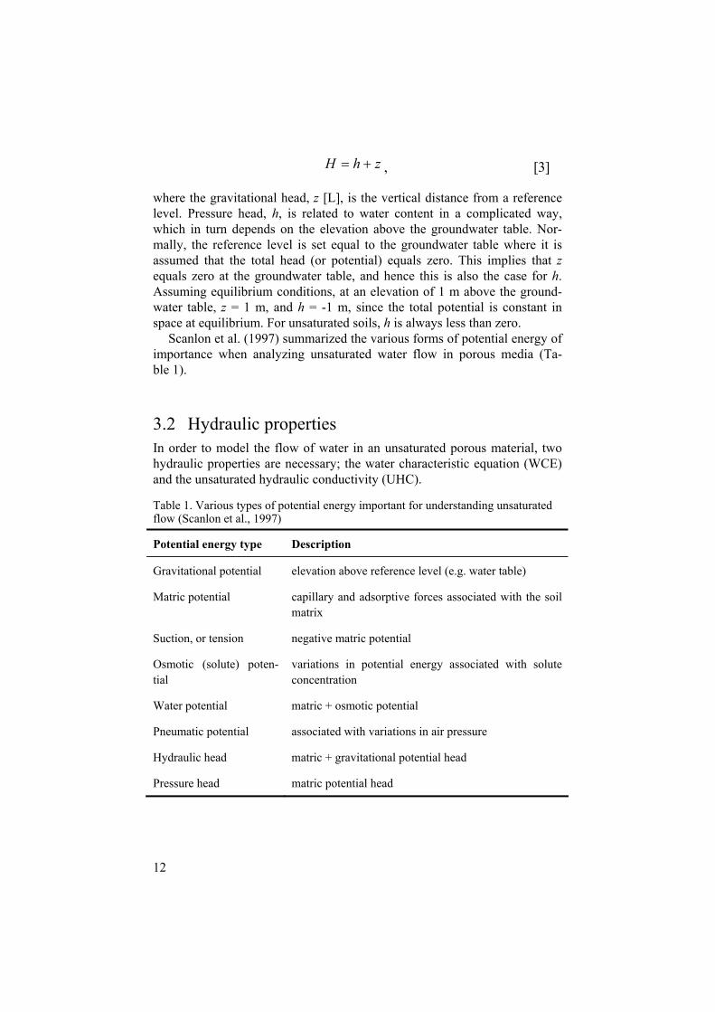
Figure 1. Model of water characteristic equation consisting of capillary tubes (left) and the resulting water characteristic curve (from Kutilek and Jensen, 1994).

3.2.1 Water characteristic equation As mentioned above, w is often expressed in terms of pressure head, h. The relation h( ) predicts the equilibrium relation between the hydraulic head and the volumetric water content, [-], and is referred to as the water charac-teristic equation in this thesis (Fig. 1). Several different notations exist, both considering the variable h, and the curve itself. Sometimes h is called suction or tension instead of pressure. Furthermore, pressure is sometimes presented as being negative, and in other cases positive. The curve itself has several names, and may e.g. be referred to as a soil water characteristic curve, a soil moisture characteristic curve, a water retention curve, a capillary pressure curve, or a pF-curve. The equations used to describe this relationship are strongly non-linear. To make it more complicated, the relation between pres-sure head and water content shows a hysteretic behaviour, which generally decreases the rate of change in as an effect of changing potential (Kutilek and Nielsen, 1994). The maximum water content of a porous medium is equal to the porosity and referred to as saturation water content, s. However, the apparent saturation water content might be less than the theoretical satu-ration water content because of air entrapment. Further, the soil never be-comes completely dry since there is always some water retained on particle surfaces. The minimum water content is called residual water content and denoted by r. Another commonly used variable is the effective saturation, Se, defined by

14

rs

reS , [4]

which equals 0 at the residual water content, and 1 at saturation. To deter-mine a water characteristic curve, field or laboratory experiments are needed. This is often a time-consuming and thus costly procedure (e.g. Wösten et al., 2001). Field methods usually require the use of tensiometers (or other methods of determining the soil water potential) and access tubes into the soil profile for measuring by a suitable technique. It is advanta-geous to measure under a specified condition such as drainage since this will give a unique relation between h and . If conditions are not controlled, the hysteretic effects will lead to scattered values representing a family of scan-ning curves.

A classical WCE is

hh

S ee , [5]

presented by Brooks and Corey (1964). Here, he [L] represents the bubbling pressure, and the pore-size index.

The equation of van Genuchten (1980) is defined as

mneh

S1

1 , [6]

where [L-1], n and m are empirical parameters. Hence, to determine the values of the parameters, the equation must be fitted to measured values of water content and pressure.

3.2.2 Permeability and hydraulic conductivity Permeability, Kp, is a property of the porous material alone, and is therefore the same for all fluids. The dimension of Kp is [L2], which corresponds to a representative pore cross-sectional area (Kutilek and Nielsen, 1994). Kp take on different forms depending on what approximation of the pore space is chosen. One example of a permeability function is the Kozeny equation

2

3

m

sp A

cK , [7]

15

where c is a shape factor [-], the tortuosity [-], and Am [L-1] the specific surface (Kutilek and Nielsen, 1994). Hence, Eq. [7] demonstrates how the permeability depends only on material specific properties. In contrast, the hydraulic conductivity of a porous medium depends on which fluid is stud-ied, as well as temperature. The relationship between permeability and satu-rated hydraulic conductivity, Ks [MT-1], is given by

gKK ps , [8]

where is the density of the fluid [ML-3], g the acceleration of gravity [LT-2], and µ the dynamic viscosity [ML-1T-1], which generally is strongly temperature dependent (Kutilek and Nielsen, 1994). In this study, hydraulic conductivity is the preferred property and will be further discussed in the next section.

3.2.3 Unsaturated hydraulic conductivity In groundwater modelling the hydraulic conductivity at saturation is used. However, as the water content is reduced, the hydraulic conductivity de-creases dramatically. Studying soils or roads (which are designed to be fairly dry compared to natural soils), predictive functions of unsaturated hydraulic conductivity are essential. The two most popular models of unsaturated hy-draulic conductivity in porous media were proposed by Burdine (1953) and Mualem (1976). Burdine hypothesized that the soil pore space was well ap-proximated using a suitable combination of cylinders with different radius, called capillary bundles. He suggested that the capillary bundles consisted of cylinders in parallel. Mualem however, suggested that the cylinders should be modelled in series instead since a small capillary connected to a large one, would control the flow. In 1980, van Genuchten showed how the WCE of Brooks and Corey (1964), and a new equation (later known as van Genuchten’s equation; Eq. [6]), could be used to obtain closed-form analyti-cal equations of unsaturated hydraulic conductivity as a function of water content using Mualem’s conductivity model. The models work reasonably well for many coarse-textured soils and other porous media having relatively narrow pore-size distributions. Predictions for many fine-textured and struc-tured soils remain inaccurate (van Genuchten et al., 1991). Nevertheless, predictive equations are often considered as the only way of characterizing large areas of land when considering the time-consuming process of meas-urements and the natural variability of soils. For site- or material-specific problems it may still be cost-effective to do measurements.

Mualem presented the following expression for calculating the unsatu-rated hydraulic conductivity:

16

2

1fSf

SKSK eleseLh , [9]

where

eS

e dxxh

Sf0

1 , [10]

where l [-] is the pore-connectivity parameter. Mualem found that l = 0.5 was a good estimate for many soils. Combining Eqs. [9] and [10] with Eq. [6] of van Genuchten while keeping m and n independent, yields

2,qpISKSK leseLh , [11]

where I is the incomplete beta-function, = Se1/m, p = m+1/n, and q = 1-1/n.

Assuming that m = 1-1/n, van Genuchten (1980) managed to derive the com-monly used closed -form equation

2111 mme

leseLh SSKSK , [12]

which obviously is much less flexible than Eq. [11] due to the restrictions put on parameters m and n. If Eq. [9] is combined with the Brooks and Corey characteristic curve, the resulting expression is

22leseLh SKSK . [13]

A recent study suggests that the measured Ks which traditionally has been inserted in Eq. [12] should be replaced with K0 being about one order of magnitude smaller than Ks, and that the value of l might deviate significantly from 0.5, and in fact should be close to -1 for most soils (Schaap and Leij, 2000). The authors emphasize that the suggested changes improve the pre-dictive power of Eq. [12] and that K0 and the new value suggested for l are of empirical nature and lack a physical base.

3.2.4 The effect of ice on hydraulic conductivityOwing to the fact that when the water in some pores are replaced with ice, the resistance to liquid water flow increases as parts of the pore space are effectively blocked by ice. Hence, the hydraulic conductivity becomes re-duced. This blocking effect is often taken into account using an impedence

17

factor, , (Lundin, 1990), which in combination with the unfrozen hydraulic conductivity, KLh, yields the frozen hydraulic conductivity, KfLh, as follows:

LhQ

fLh KK 10 , [14]

where Q represents the fraction of unfrozen water. Furthermore, Stähli et al. (1996) showed that in relation to infiltration events, the hydraulic conductiv-ity in frozen soil should be modified to take into account the fact that the pore space on such occasions is divided into three (or more) fractions: small pores with unfrozen water, midsize pores with frozen pores, and large pores where most of the infiltrated water find its way. Thus, the hydraulic conduc-tivity under such circumstances is not solely defined by the unfrozen water content in the small pores which are available before infiltration, but the hydraulic conductivity increases quickly, and step-like, as the larger pores become water filled.

3.2.5 Prediction of soil hydraulic properties Due to the often difficult, costly, and time-consuming process of measuring hydraulic properties, various methods to predict the hydraulic properties have been developed. The objective is to transfer available data into data needed. Bouma (1989) named these methods pedo-transfer functions (PTF). According to Wösten et al. (2001) three types of PTFs can be distinguished:

3.2.5.1 Method 1: Prediction of hydraulic properties based on soil structural models.

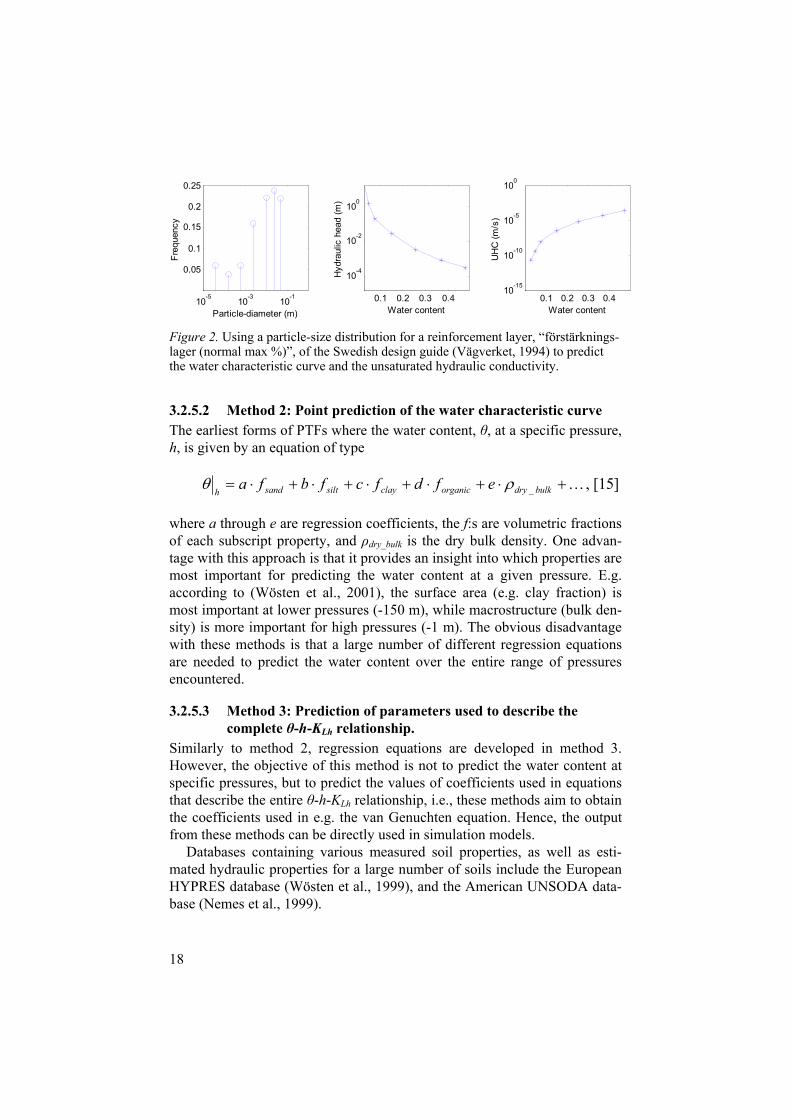
Arya and Paris (1981) presented a model that predicts the WCE from the particle-size distribution, bulk density and particle density. The original model has been modified over the years, and predicts the WCE well for sandy soils, while it is less accurate for loamy and clayey soils (Wösten et al., 2001). By means of adjusting bulk density, the effect of packing can easily be accounted for, which makes the Arya-Paris method particularly interesting in road applications. It is likely that it will work well even for the coarser materials commonly used in road constructions (Arya 2003, personal communication). The Arya-Paris model predicts the -h-KLh relationship at pressures corresponding to the particle classes as defined by the measured particle-sizes (Fig. 2). In paper III, the Arya-Paris model was used to esti-mate hydraulic properties for a few layers in a model road structure.

18

10-5

10-3

10-1

0.05

0.1

0.15

0.2

0.25

Particle-diameter (m)

Freq

uenc

y

0.1 0.2 0.3 0.4

10-4

10-2

100

Hyd

raul

ic h

ead

(m)

Water content0.1 0.2 0.3 0.4

10-15

10-10

10-5

100

UH

C (m

/s)

Water content

Figure 2. Using a particle-size distribution for a reinforcement layer, “förstärknings-lager (normal max %)”, of the Swedish design guide (Vägverket, 1994) to predict the water characteristic curve and the unsaturated hydraulic conductivity.

3.2.5.2 Method 2: Point prediction of the water characteristic curve The earliest forms of PTFs where the water content, , at a specific pressure, h, is given by an equation of type

bulkdryorganicclaysiltsandhefdfcfbfa _ , [15]

where a through e are regression coefficients, the f:s are volumetric fractions of each subscript property, and dry_bulk is the dry bulk density. One advan-tage with this approach is that it provides an insight into which properties are most important for predicting the water content at a given pressure. E.g. according to (Wösten et al., 2001), the surface area (e.g. clay fraction) is most important at lower pressures (-150 m), while macrostructure (bulk den-sity) is more important for high pressures (-1 m). The obvious disadvantage with these methods is that a large number of different regression equations are needed to predict the water content over the entire range of pressures encountered.

3.2.5.3 Method 3: Prediction of parameters used to describe the complete -h-KLh relationship.

Similarly to method 2, regression equations are developed in method 3. However, the objective of this method is not to predict the water content at specific pressures, but to predict the values of coefficients used in equations that describe the entire -h-KLh relationship, i.e., these methods aim to obtain the coefficients used in e.g. the van Genuchten equation. Hence, the output from these methods can be directly used in simulation models.

Databases containing various measured soil properties, as well as esti-mated hydraulic properties for a large number of soils include the European HYPRES database (Wösten et al., 1999), and the American UNSODA data-base (Nemes et al., 1999).

19

3.3 Thermal properties 3.3.1 Thermal conductivity According to Chung and Horton (1987), the apparent thermal conductivity for unfrozen conditions, ( ) [W m-1K-1, MLT-3K-1], can be described by

5.03210

0

bbb

qC wwt

, [16a, b]

where 0( ) is the thermal conductivity of the porous medium (solid plus wa-ter) in the absence of flow, t is the longitudinal thermal dispersivity [L], and b1, b2, and b3 are empirical parameters [MLT-3K-1] that vary with material. Instead of Eq. [16b], the expression of Campbell (1985) can be used

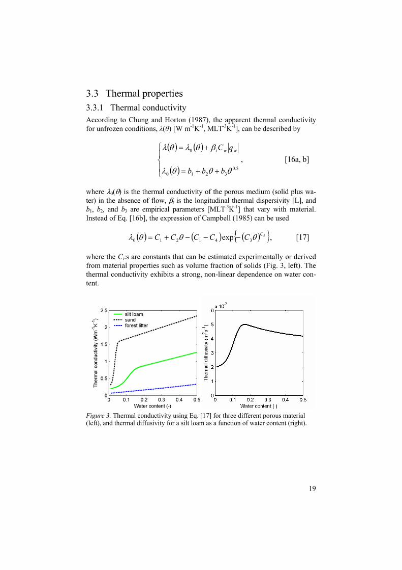
5341210 exp CCCCCC , [17]

where the Ci:s are constants that can be estimated experimentally or derived from material properties such as volume fraction of solids (Fig. 3, left). The thermal conductivity exhibits a strong, non-linear dependence on water con-tent.

Figure 3. Thermal conductivity using Eq. [17] for three different porous material (left), and thermal diffusivity for a silt loam as a function of water content (right).

20

3.3.2 Heat capacity The volumetric heat capacity of moist soil, Cp [ML-1T-2 K-1, Jm-3K-1], is tra-ditionally defined as the sum of the volumetric heat capacities of solids, Cn,liquid water, Cw, vapour, Cv, and ice, Ci, multiplied by their respective volu-metric fractions :

p n n w v v i iC C C C C [18]

3.3.3 Thermal diffusivity Thermal diffusivity may be looked upon as the best measure of how quickly temperature changes are transferred through the porous material. Thermal diffusivity is defined as the quotient of thermal conductivity and heat capac-ity. Typically, the thermal diffusivity curve is very non-linear, with a pro-nounced maximum caused by the very non-linear increase in thermal con-ductivity (Fig. 3, right).

3.4 Freezing and thawing 3.4.1 The unresolved problem of freezing Freezing and thawing of water within a porous material have been studied since the late 1800s, and a common way to deal with the problem in simula-tion models has been to make use of thermodynamic theories. In spite of the long history of research in the field, the thermodynamic theory of soil freez-ing presents a problem that has thus far not been solved. Similarly to vapori-zation, freezing couples the heat and water transport equations since latent heat (energy) is required for water to change between its phases (ice, liquid, vapour). The Clapeyron equation postulates the relation between the re-quired changes in pressure and temperature in order to maintain two phases at equilibrium

TL

dTdP fw , [19]

where P is the pressure [Pa, ML-1T-2] (= wgh), Lf is the latent heat of freez-ing [Jkg-1K-1, L2T-2], w is the density of liquid water [ML-3] (~1,000 kg m-3),and T is the temperature [K] (Alberty and Silbey, 1992). The interpretation of the equations is as follows: both phases (e.g. ice and liquid water) will continue to exist at equilibrium only if pressure and temperature are changed in such a way that the Clapeyron equation is satisfied. Kay and Groenevelt

21

(1974) and Groenevelt and Kay (1974) derived several Clapeyron equations based on Eq. [19] relating the various phases of water to each other. How-ever, one of these has been by far mostly used, namely the generalized Clapeyron equation being used in a similar form as early as 1935 by Schofield. Often, the effects of solutes on freezing (osmotic effects) are in-cluded in the equation, which after integration and conversion to head units finally results in

gicRTh

TT

gL

hw

ii

wf

0

ln , [20]

where T0=273.15 K, i is the density of ice, hi is the ice pressure head, i is the van’t Hoff, or osmotic, coefficient [-], c the concentration of the solute [moles m-3], and R the universal gas constant [J moles-1 K-1] (e.g. Mizoguchi, 1993; Nieber et al., 1997). Finally, the problem referred to in the heading of this section is unfolded in Eq. [20]; videlicet, we have one equation but two unknowns: h, and hi. As a result of this seemingly impossible situation, two schools have developed over the years; one in which the liquid water pres-sure is neglected, and one in which the ice pressure is neglected. In this the-sis, the models of the first school are named Miller-type models, while the models of the other school are named hydrodynamic models. They will be discussed further in the next two sections of this chapter. To the best knowl-edge of the author, no solution to this problem has been presented in terms of a computer code where both ice and liquid pressure are realistically ac-counted for.

3.4.2 Miller-type models The Miller-type models make assumptions about the pressure head in order to reduce the number of unknowns in Eq. [20] to one. The most common approximation is to assume that the pressure head is always zero which ob-viously is not the case in an unsaturated soil. The strength of these models is that the ice pressure is allowed to change, and thus they can be used to pre-dict frost heave in a physically realistic way on the microscopic scale. How-ever, the macroscopic scale process which fuels the frost heave mechanism is the freezing-induced redistribution of water caused by the “capillary sink” formed upon the conversion of liquid water to ice (Miller, 1980). Hence, in order to develop frost heave models, one must assume a static pressure head, which contradicts the statement about the change in pressure head (the capil-lary sink) necessary to explain the frost induced redistribution of water – a paradox. Nevertheless, the theories of these models are useful in describing (although in a simplified way with respect to hydraulics) the physics of frost heave on the microscopic scale, and contribute to the understanding of which

22

factors are important to consider when trying to reduce frost heave in e.g. roads, airfields or similar structures. One example is the rigid-ice model presented in O’Neill and Miller (1985), which includes the concept of sec-ondary heaving in addition to the firstly developed primary heaving also known as the Taber-Beskow model, or Everett model (Miller, 1980). Frost heave is usually associated with the formation of segregated ice, i.e. upon freezing of the pore water, the soil particles are excluded such that the vol-umes of ice in the soil are segregated from the soil, which in relatively in-compressible soils leads to ice lens formation, while in more compressible soils, the ice is formed in complex networks of ice (Miller, 1980). Ice lenses are discrete, soil free lenses of pure ice, which generally form perpendicular to the thermal gradient (e.g. Miller, 1980; Watanabe and Mizoguchi, 2000). Recently, Rempel et al. (2004) presented a paper in which they managed to replace the “ad hoc” partitioning of total stress used by O’Neill and Miller (1985) with an exact integral expression for the frost heaving pressure. Rempel et al. (2004) conclude that the fluid pathways in the frozen soil de-pend on the freezing mechanisms described by the Clapeyron equation, while long-range inter-molecular forces (e.g. van der Waals forces) govern frost heave. Similarly, Watanabe and Mizoguchi (2002) found that the amount of unfrozen water in a saturated material could be estimated based on the theories of van der Waals forces, Coulombic interactions, and the Gibbs-Thomson effect. However, application of these theories requires knowledge of the materials’ microscopic characteristics such as the surface area which is rarely available in practice.

In conclusion, Miller-type models are useful in explaining the physics of frost heave on the microscopic scale, and macroscopic scale models are use-ful in approximating frost heave. So far though, the former models have been difficult to apply in practice.

3.4.3 Hydrodynamic models In contrast to the Miller-type models, the hydrodynamic models ignore changes in ice pressure, and simply assume that the ice pressure is zero, which is incorrect where ever frost heave occurs (e.g. Miller, 1980). How-ever, when validating the hydrodynamic models against laboratory or field data, they generally perform well, which led Spaans and Baker (1996) to conclude that “the broad assumption of zero gauge pressure in the ice phase has been questioned under certain conditions (Miller, 1973; 1980), but thus far there is scant evidence against it, except in obvious cases (heaving)”. It is furthermore likely, that for most soil physicists, the hydrodynamic models are easier to comprehend than the Miller-type models, as they fit nicely into e.g. the Richards’ equation. As a result, the hydrodynamic formulations have been the more popular choice in most models that aim to simulate the cou-pled transport of heat and water in porous materials. Some hydrodynamic

23

models even predict frost heave to occur when the ice content becomes lar-ger than a specified portion of the pore space, e.g. 90% of porosity as sug-gested by the experiments of Dirksen and Miller (1966) presented in Miller (1980). Such predictions do not have a proper physical base, but may still provide useful approximations of reality.

Using the theory of the hydrodynamic models, the water and heat trans-port equations are modified to include the phase change between water and ice. In paper I, the one-dimensional water flow and heat flux equations pro-vide examples of a hydrodynamic model (Eqs. [22], and [23]).

3.5 Measurements of water content in granular materials

3.5.1 A short review of methods to measure hydraulic properties

The most basic method of measuring water content in a porous material is to weigh a sample, dry it in an oven, weigh it again and from the weight differ-ence calculate the initial water content of the sample. However, the gravim-etric method is destructive in requiring that samples are collected from the road/soil and brought into the laboratory. Furthermore, since it is a destruc-tive method, it only provides information for a single moment in time, and is thus not suitable for monitoring. Instead, the gravimetric method has become the standard method used to evaluate or calibrate other methods since it is considered the most reliable (e.g. Shaw, 1994). When evaluating simulations of water content, year-long time-series from sensors fixed in space are needed. Measurements of water content or perhaps tension in the unsaturated zone as well as the depth to the groundwater table are desired. In addition, thermal data like temperature, or heat flux, is crucial in cold climates since the water and energy states of the materials are intimately linked (comp. chapter 4). However, in this thesis, the discussion is restricted to methods directly related to hydraulic properties.

To measure the location of the groundwater table a vertical tube in the road/soil is needed, and a device to measure either the pressure from the water column above it, or a device that measures the distance from the top of the tube to the water table. It is far more complicated to determine the un-saturated water content, even though some groundwater tubes exhibit meas-urement difficulties due to freezing during the winter. The most widely used method for continuous monitoring of unsaturated water content in roads is the time domain reflectometry (TDR) method (Svensson, 1997). Other methods include neutron probes, water content reflectometers (WCR), and electrical resistance blocks.

24

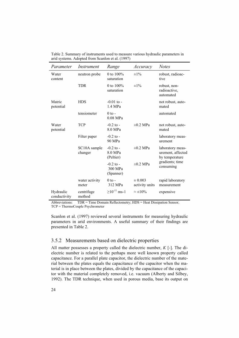
Table 2. Summary of instruments used to measure various hydraulic parameters in arid systems. Adopted from Scanlon et al. (1997)

Parameter Instrument Range Accuracy Notes neutron probe 0 to 100%

saturation ±1% robust, radioac-

tive Watercontent

TDR 0 to 100% saturation

±1% robust, non-radioactive, automated

HDS -0.01 to -1.4 MPa

not robust, auto-mated

Matricpotential

tensiometer 0 to -0.08 MPa

automated

TCP -0.2 to -8.0 MPa

±0.2 MPa not robust, auto-mated

Filter paper -0.2 to -90 MPa

laboratory meas-urement

-0.2 to -8.0 MPa (Peltier)

±0.2 MPa SC10A sample changer

-0.2 to - 300 MPa (Spanner)

±0.2 MPa

laboratory meas-urement, affected by temperature gradients; time consuming

Waterpotential

water activity meter

0 to - 312 MPa

± 0.003 activity units

rapid laboratory measurement

Hydraulic conductivity

centrifuge method

10-11 ms-1 ±10% expensive

Abbreviations: TDR = Time Domain Reflectometry; HDS = Heat Dissipation Sensor; TCP = ThermoCouple Psychrometer

Scanlon et al. (1997) reviewed several instruments for measuring hydraulic parameters in arid environments. A useful summary of their findings are presented in Table 2.

3.5.2 Measurements based on dielectric properties All matter possesses a property called the dielectric number, K [-]. The di-electric number is related to the perhaps more well known property called capacitance. For a parallel plate capacitor, the dielectric number of the mate-rial between the plates equals the capacitance of the capacitor when the ma-terial is in place between the plates, divided by the capacitance of the capaci-tor with the material completely removed, i.e. vacuum (Alberty and Silbey, 1992). The TDR technique, when used in porous media, base its output on

25

the dielectric number of the granular material, positioned not between paral-lel plates, but between metal rods positioned in various geometrical configu-rations. It does not measure the dielectric number directly, but instead uses the principle that the velocity of an electromagnetic wave depends on the dielectric number of the material that it travels through. Hence, an electro-magnetic wave is transmitted along the metal rods, which acts as wave guides, and depending on the dielectric number, the time required for the wave to travel along the rods and back varies (e.g. Nissen and Møldrup, 1995). The travel time can then be related to an apparent dielectric number of the granular material, which subsequently can be related to the volumetric water content using various methods (Yu et al., 1999; Jacobsen and Schjønning, 1995). In contrast, the so called capacitance technique measures the capacitance of the surrounding granular material at discrete depths through an access tube (e.g. Seyfried and Murdock, 2001; Baumhardt et al., 2000), i.e. it is not in direct contact with the material like sensors in the TDR technique are. However, it uses the basic relation between capacitance and dielectric number described above, although a geometrical factor must be introduced since the material is not simply placed between two parallel plates (e.g. Dean et al., 1987).

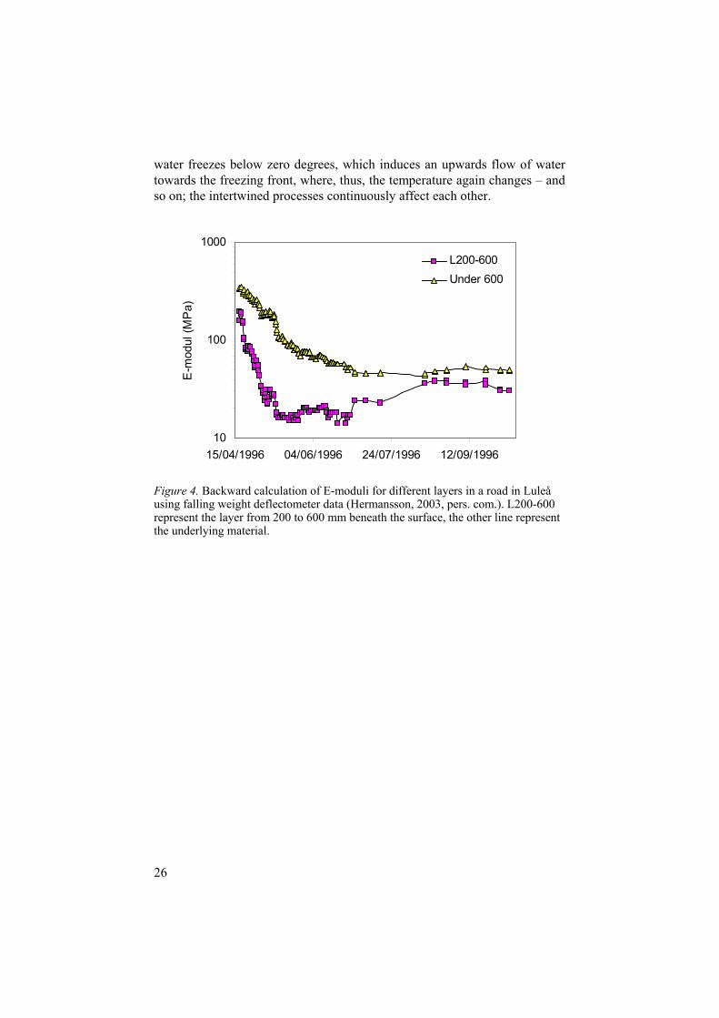
3.6 Effects of water content variations on road damage It was mentioned in the introduction that the material properties that are im-portant to consider when studying the degradation of roads are affected by temperature and water content. In numerical models used to predict road degradation, the elastic modulus, which is the governing material property, typically takes on fixed values according to season; summer, autumn, winter, thaw, and spring (Vägverket, 1994). The impact of season on elastic modulus can be quite dramatic (Fig. 4), as it depends on water and ice con-tent within the materials where high water contents affect the load tolerance in a negative way, while ice in general act to reinforce the road. However, during spring thaw weakening, ice in lower layers creates problems since it is blocking parts of the percolation pathways, thus restricting the possibilities for the melt water in the top layers to flow downwards. As a consequence of the unusually high water contents, the road may suffer an almost complete loss of strength, leading to thaw settling, formation of potholes and similar problems (e.g. Miller, 1980). During most of the year, the road structure suffers little damage, and most of the yearly deterioration actually occurs during a few days, in particular during spring thaw weakening, or during hot summer days when the asphalt layer can be heavily deformed as a result of the combination of high temperature, and heavy or long lasting loads (Whiteoak, 1990). Apparently, when studying road structures in cold cli-mates it is necessary to consider water and heat transport concurrently since

26

water freezes below zero degrees, which induces an upwards flow of water towards the freezing front, where, thus, the temperature again changes – and so on; the intertwined processes continuously affect each other.

10

100

1000

15/04/1996 04/06/1996 24/07/1996 12/09/1996

E-m

odul

(MP

a)

L200-600Under 600

Figure 4. Backward calculation of E-moduli for different layers in a road in Luleå using falling weight deflectometer data (Hermansson, 2003, pers. com.). L200-600 represent the layer from 200 to 600 mm beneath the surface, the other line represent the underlying material.

27

4 Modelling approach

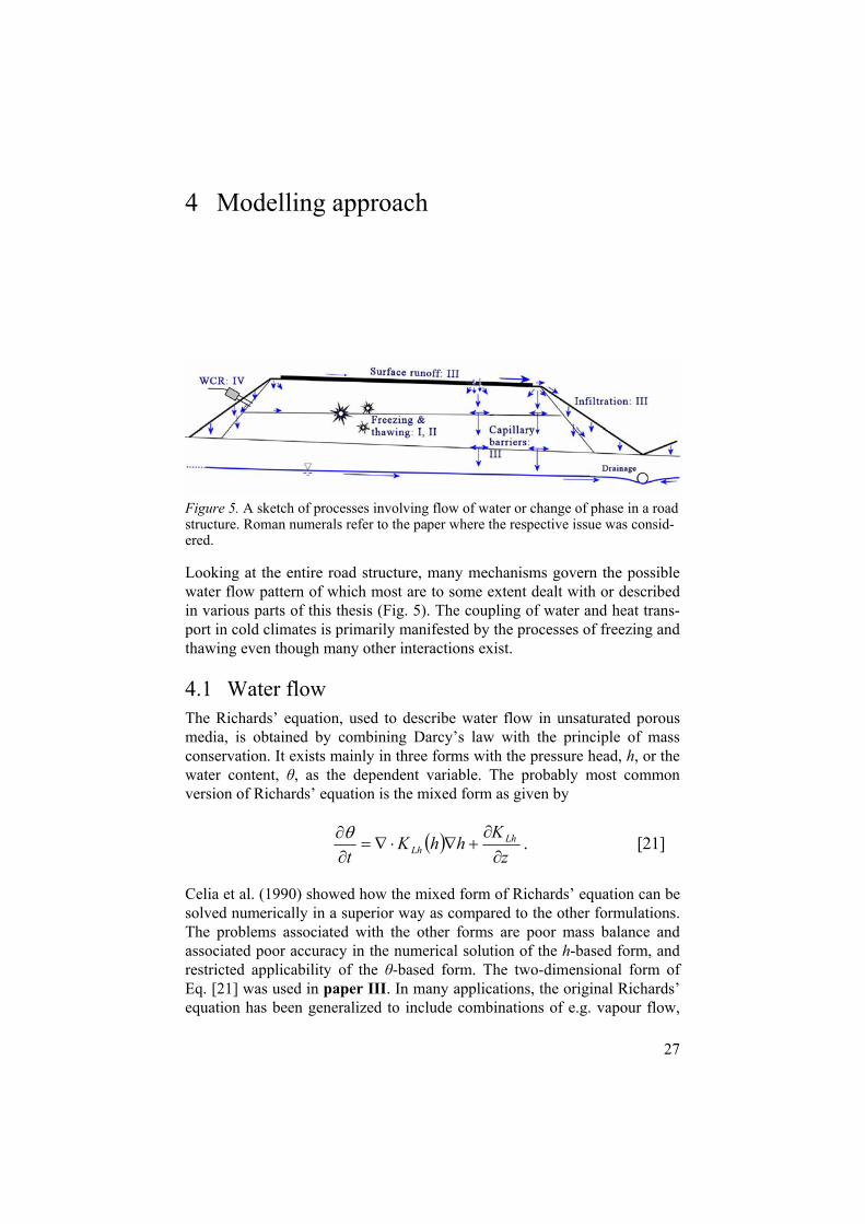
Figure 5. A sketch of processes involving flow of water or change of phase in a road structure. Roman numerals refer to the paper where the respective issue was consid-ered.

Looking at the entire road structure, many mechanisms govern the possible water flow pattern of which most are to some extent dealt with or described in various parts of this thesis (Fig. 5). The coupling of water and heat trans-port in cold climates is primarily manifested by the processes of freezing and thawing even though many other interactions exist.

4.1 Water flow The Richards’ equation, used to describe water flow in unsaturated porous media, is obtained by combining Darcy’s law with the principle of mass conservation. It exists mainly in three forms with the pressure head, h, or the water content, , as the dependent variable. The probably most common version of Richards’ equation is the mixed form as given by

zK

hhKt

LhLh . [21]

Celia et al. (1990) showed how the mixed form of Richards’ equation can be solved numerically in a superior way as compared to the other formulations. The problems associated with the other forms are poor mass balance and associated poor accuracy in the numerical solution of the h-based form, and restricted applicability of the -based form. The two-dimensional form of Eq. [21] was used in paper III. In many applications, the original Richards’ equation has been generalized to include combinations of e.g. vapour flow,

28

coupling effects, and phase change (e.g. Harlan, 1973; Flerchinger and Saxton, 1989; Šim nek et al., 1998; Jansson and Karlberg, 2004). Another example is the generalized Richards’ equation in one dimension as described in paper I

flowvapour

vTvh

flowliquid

LTLhLh

i

w

iu

zTK

zhK

zThKhK

zhhK

z

tT

th

[22]

where u is the volumetric unfrozen water content [L3L-3] (= + v), is the volumetric liquid water content [L3L-3], v is the volumetric vapour content expressed as an equivalent water content [L3L-3], i is the volumetric ice con-tent [L3L-3], t is time [T], z is the spatial coordinate positive upward [L], i is the density of ice ( 931 kg m-3). This version of the Richards’ equation ex-hibits strong temperature dependence as well as a hydraulic dependence. Water flow in Eq. [22] is assumed to be caused by five different processes with corresponding hydraulic conductivities (given below in parentheses). The first three terms on the right-hand side of Eq. [22] represent liquid flows due to a pressure head gradient (KLh, [LT-1]), gravity, and a temperature gra-dient (KLT, [L2T-1K-1]), respectively. The next two terms represent vapour flows due to pressure head (Kvh, [LT-1]) and temperature (KvT, [L2T-1K-1]) gradients, respectively. KLh, the unsaturated hydraulic conductivity, was described in detail earlier. The vapour conductivities are described in Fayer (2000) and Scanlon et al. (2003). The hydraulic conductivity KLT for liquid phase fluxes due to a gradient in T is defined in e.g. Fayer (2000), and No-borio et al. (1996). Equation [22] is highly nonlinear, mainly due to depend-encies of the water content and the hydraulic conductivity on the pressure head, i.e., (h) and KLh(h), respectively, and due to freezing/thawing effects that relate the ice content to the temperature, i.e., i(T). It contains conduc-tivities that depend on temperature, as well as a direct influence on water flow and water phase by temperature gradients. In situations where Eq. [22] is solved simultaneously with the heat equation, the combined model is said to be coupled since heat and water flows depend on each other.

29

4.2 Heat flux Within the road structure, heat is transported by conduction as described by Fourier’s law or by transport with water and vapour flow respectively. This makes the heat transport equation slightly more complicated as it comprises convection as well as diffusion. A change in heat, or energy, at a given point in any porous medium does not automatically lead to a change in tempera-ture since it may also lead to phase changes. The heat transported by conduc-tion through the matrix or by water flow is referred to as sensible heat, and the heat transported by vapour as latent heat. Heat transport due to vapour flow is named latent since a thermometer is unable to register a change in temperature until the vapour condensates and releases sensible heat, which can be detected directly. When dealing with frozen conditions, one of the main concerns is how to partition the change in energy between latent and sensible heat. Heat transport during transient flow in a variably-saturated porous medium is described as (e.g., Nassar and Horton, 1989; 1992; pa-per I):

zq

TLzTq

CzTq

CzT

z

tT

TLt

LtTC

vvv

lw

viif

p

0

0

, [23]

where Lf is the latent heat of freezing (~3.34·105 Jkg-1), L0 is the volumetric latent heat of vaporisation of water [Jm-3, ML-1T-2], L0 = Lw w, Lw is the latent heat of vaporisation of water [Jkg-1] (=2,501.106-2,369.2·T [˚C]), and ql[LT-1] and qv [LT-1] represent the flow of liquid water and vapour respec-tively. The first term on the left-hand side represents changes in the sensible energy content, and the second and third terms represent changes in the la-tent heat of the ice and vapour phases, respectively. The terms on the right-hand side represent respectively soil heat flow by conduction, convection of sensible heat with flowing water, transfer of sensible heat by diffusion of water vapour, and transfer of latent heat by diffusion of water vapour. Notice that there is a strong coupling to the water flow equation through all terms on the right hand side, as well as on the left hand side due to phase changes of wa-ter.

4.3 Apparent volumetric heat capacity When modelling systems where freezing and thawing occurs, the concept of apparent heat capacity, Ca, is often introduced. Harlan (1973) described how

30

the first two terms of Eq. [23] can be merged into one by means of the ap-parent heat capacity according to

dTd

LCC iifpa . [24]

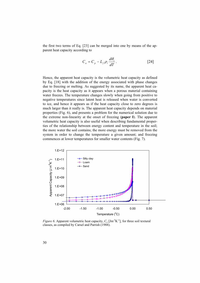
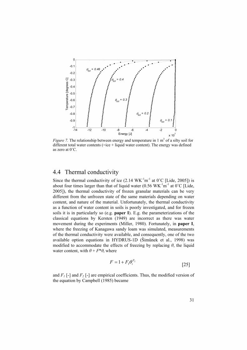
Hence, the apparent heat capacity is the volumetric heat capacity as defined by Eq. [18] with the addition of the energy associated with phase changes due to freezing or melting. As suggested by its name, the apparent heat ca-pacity is the heat capacity as it appears when a porous material containing water freezes. The temperature changes slowly when going from positive to negative temperatures since latent heat is released when water is converted to ice, and hence it appears as if the heat capacity close to zero degrees is much larger than it really is. The apparent heat capacity depends on material properties (Fig. 6), and presents a problem for the numerical solution due to the extreme non-linearity at the onset of freezing (paper I). The apparent volumetric heat capacity is also useful when describing fundamental proper-ties of the relationship between energy content and temperature in the soil; the more water the soil contains; the more energy must be removed from the system in order to change the temperature a given amount; and freezing commences at lower temperatures for smaller water contents (Fig. 7).

1.E+06

1.E+07

1.E+08

1.E+09

1.E+10

1.E+11

1.E+12

-2.00 -1.50 -1.00 -0.50 0.00 0.50

Temperature (oC)

App

aren

t Cap

acity

(J m

-3K

-1) Silty clay

LoamSand

Figure 6. Apparent volumetric heat capacity, Ca [Jm-3K-1], for three soil textural classes, as compiled by Carsel and Parrish (1988).

31

-14 -12 -10 -8 -6 -4 -2 0

x 107

-1

-0.9

-0.8

-0.7

-0.6

-0.5

-0.4

-0.3

-0.2

-0.1

0

Energy [J]

Tem

pera

ture

[deg

rees

C]

tot = 0.46

tot = 0.4

tot = 0.3

tot = 0.2

tot = 0.1

Figure 7. The relationship between energy and temperature in 1 m3 of a silty soil for different total water contents (=ice + liquid water content). The energy was defined as zero at 0˚C.

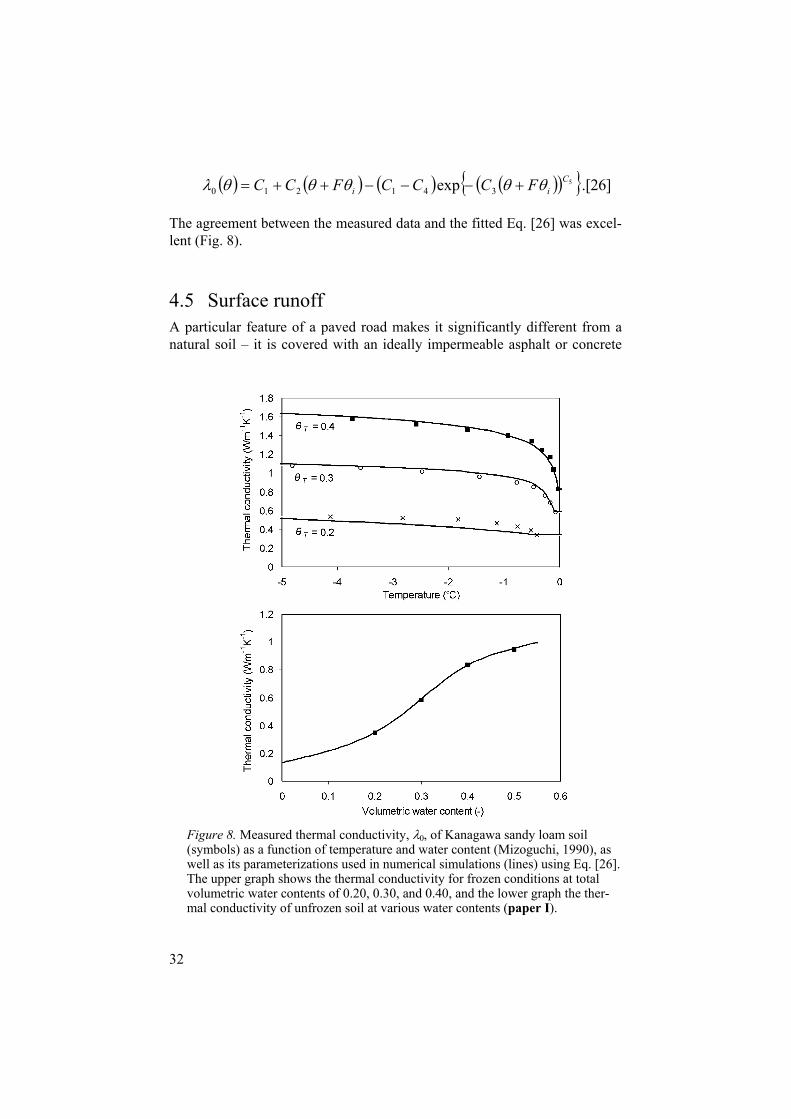
4.4 Thermal conductivity Since the thermal conductivity of ice (2.14 WK-1m-1 at 0˚C [Lide, 2005]) is about four times larger than that of liquid water (0.56 WK-1m-1 at 0˚C [Lide, 2005]), the thermal conductivity of frozen granular materials can be very different from the unfrozen state of the same materials depending on water content, and nature of the material. Unfortunately, the thermal conductivity as a function of water content in soils is poorly investigated, and for frozen soils it is in particularly so (e.g. paper I). E.g. the parameterizations of the classical equations by Kersten (1949) are incorrect as there was water movement during the experiments (Miller, 1980). Fortunately, in paper I,where the freezing of Kanagawa sandy loam was simulated, measurements of the thermal conductivity were available, and consequently, one of the two available option equations in HYDRUS-1D (Šim nek et al., 1998) was modified to accommodate the effects of freezing by replacing , the liquid water content, with + F* i where

211 F

iFF [25]

and F1 [-] and F2 [-] are empirical coefficients. Thus, the modified version of the equation by Campbell (1985) became

32

5341210 exp C

ii FCCCFCC .[26]

The agreement between the measured data and the fitted Eq. [26] was excel-lent (Fig. 8).

4.5 Surface runoffA particular feature of a paved road makes it significantly different from a natural soil – it is covered with an ideally impermeable asphalt or concrete

Figure 8. Measured thermal conductivity, 0, of Kanagawa sandy loam soil (symbols) as a function of temperature and water content (Mizoguchi, 1990), as well as its parameterizations used in numerical simulations (lines) using Eq. [26]. The upper graph shows the thermal conductivity for frozen conditions at total volumetric water contents of 0.20, 0.30, and 0.40, and the lower graph the ther-mal conductivity of unfrozen soil at various water contents (paper I).

33

layer. Contrary to the soil (in most cases), the result is a diversion of precipi-tated water along the surface causing surface runoff with a focused infiltra-tion in the shoulder (e.g. paper III). Surface runoff can be calculated using a combination of the kinematic wave equation (e.g. Jaber and Mohtar, 2002)

txrxq

th , , [27]

and Manning’s equation for a channel of unit width

MhSq

355.0

, [28]

where h [L] is the water depth on the surface, q [L2T-1] is the water flow per unit width along the surface, S [-] is the slope of the surface, r [LT-1] is the source (precipitation - infiltration) and M [L-1/3T1] is Manning’s roughness coefficient accounting for the hydraulic resistance of the road surface. A suitable M value for asphalt is 0.016 and for gravel 0.025 (Crowe et al., 2001).

4.6 Fracture zone water flow Even though the paved road is intended to be impervious to water, time will change the nature of the surface. Eventually fractures will develop in roads having an asphalt cover, in particular in the wheel paths where the load from the vehicles on average is greatest. Concrete roads always have large frac-ture-like structures as a result of the joints between the concrete slabs. If the joints are properly sealed, the concrete roads are impervious as long as the sealing is intact, but the joints are not always sealed. Due to the fact that even very small fractures have a large capability to transport water, simula-tion of water transport in a road structure with a fractured surface requires a code that allows for this process.

The HYDRUS-2D numerical code (Šim nek et al., 1999) was designed to simulate flow and transport in porous materials. While materials that are heterogeneous with respect to hydraulic properties can be simulated directly, the code do not explicitly account for fractures. However, highly fractured porous materials can be described using equivalent homogenous porous me-dia models (e.g. van der Kamp, 1992). In paper III, a study of the effect of fracture width (=aperture) on the flow patterns within the road structure as generated by rainfall was performed. In the investigation it was assumed for practical reasons that the fractured zone could be classified as highly frac-tured. Furthermore, assuming parallel fractures of identical and constant

34

aperture, the effective hydraulic conductivity of a fractured zone, Kf, can be predicted using the parallel plate model (e.g. Freeze and Cherry, 1979)

1222 3 g

BbK w

f , [29]

where 2b is the fracture aperture (= width), 2B is the distance between frac-tures, and µ is the dynamic viscosity (= 1.00·10-3 kg m-1s-1 at 20˚C). Equation [29] is useful in estimating the saturated hydraulic conductivity in a fractured zone, but the unsaturated hydraulic conductivity is still unknown. An aspect to consider in future work may be the fact that the bitumen, which acts as a glue fixing the stones in the asphalt layer, is hydrophobic, complicating things since the standard hydraulic properties are derived assuming a hydro-philic matrix. However, theory formulations dealing with these special cases of porous materials, as well as measurements and modelling of water repel-lent sands are in progress (Šim nek, 2005, pers. com.).

4.7 Numerical solutions to the water and heat transport equations

4.7.1 What is a numerical solution, and what are the benefits of numerical methods?

In short, a numerical solution consists of numerical values resulting from the application of a numerical method to a mathematical problem. In contrast, if an analytical solution to the same problem could be found, the answer would be in closed form. The first advantage of the analytical solution is that once it is established, the effect of individual parameters or boundary conditions can be immediately evaluated. Furthermore, the analytical solution is exact in contrast to the numerical solution, which is an approximation. In addition, to investigate effects of parameters or boundary conditions in the numerical solution, time consuming methods involving non-trivial elements such as the Monte Carlo method, used in paper II, is the only alternative. So, why bother about numerical solutions at all? Well, the answer is that numerical methods can be used to solve mathematical problems for which analytical solutions are impossible or exceedingly difficult to obtain, or even use. Con-sider the following problem and solution which was adapted from Bárány and Yngve (1994) and freely translated from Swedish by the author:

”Determine the stationary temperature in a homogeneous cylinder of radius a, and length L, if its plane surfaces have temperature zero, and the curved surface has temperature T0.” The solution in cylindrical coordinates is:

35

00

0

12

12

12

12sin4,

no

LanI

LrnI

nLzn

Tzru , [30]

where Io denote the modified Bessel function, which itself is a complicated function. Evidently, the solution is complicated, and even though the solu-tion in form of Eq. [30] is exact, it can never provide an exact temperature value in a specified point since that would require an infinite summation. In addition, if the cylinder has e.g. a bump somewhere on the surface, an ana-lytical solution cannot be found at all. Hence, if the stationary solution to a the heat conduction problem in a homogeneous cylinder is that complicated, it would obviously be difficult to obtain an analytical solution for the tem-perature in a heterogeneous road having a complicated geometry (at least compared to a cylinder) and that is exposed to time-variable boundary condi-tions. In conclusion, this is the reason why numerical methods exist, and why they become ever more popular. However, one should always remem-ber that numerical solutions are approximations of the true solutions, and that it requires some experience to use a numerical model in a proper man-ner.

4.7.2 MeshesAs concluded in the previous section, to solve any of the equations listed in chapter 4, a numerical method is required unless boundary conditions and material properties that are unrealistically simple in representing a road are used. There are a variety of numerical solution methods available, and whichever is the best choice depends on e.g. the numerical proficiency of the user and the problem formulation. The general principle of a numerical method is that even if the problem to be solved is defined over e.g. the road cross-sectional area, the solution variable (e.g. temperature or water content) is computed only at a limited number of points (generally referred to as nodes) belonging to the cross-section, or as average variable values in sub-areas like line segments, triangles or squares. Such a geometrical arrange-ment of the problem domain is generally referred to as a grid or mesh, and comprises the points where the solution is calculated as well as the lines connecting every point with its neighbours. To generate a mesh can be com-plicated, in particular in higher dimensions, and a number of methods are

36

1: Distribute points 2: Triangulate 3: Force equilibrium

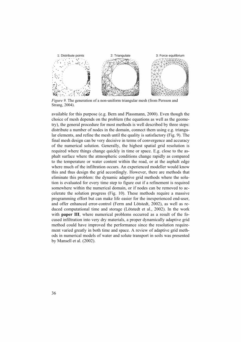
Figure 9. The generation of a non-uniform triangular mesh (from Persson and Strang, 2004).

available for this purpose (e.g. Bern and Plassmann, 2000). Even though the choice of mesh depends on the problem (the equations as well as the geome-try), the general procedure for most methods is well described by three steps: distribute a number of nodes in the domain, connect them using e.g. triangu-lar elements, and refine the mesh until the quality is satisfactory (Fig. 9). The final mesh design can be very decisive in terms of convergence and accuracy of the numerical solution. Generally, the highest spatial grid resolution is required where things change quickly in time or space. E.g. close to the as-phalt surface where the atmospheric conditions change rapidly as compared to the temperature or water content within the road, or at the asphalt edge where much of the infiltration occurs. An experienced modeller would know this and thus design the grid accordingly. However, there are methods that eliminate this problem: the dynamic adaptive grid methods where the solu-tion is evaluated for every time step to figure out if a refinement is required somewhere within the numerical domain, or if nodes can be removed to ac-celerate the solution progress (Fig. 10). These methods require a massive programming effort but can make life easier for the inexperienced end-user, and offer enhanced error-control (Ferm and Lötstedt, 2002), as well as re-duced computational time and storage (Lötstedt et al., 2002). In the work with paper III, where numerical problems occurred as a result of the fo-cused infiltration into very dry materials, a proper dynamically adaptive grid method could have improved the performance since the resolution require-ment varied greatly in both time and space. A review of adaptive grid meth-ods in numerical models of water and solute transport in soils was presented by Mansell et al. (2002).

37

0 500 1000 1500 2000 2500

500

1000

1500

2000

x

y

0 500 1000 1500 2000 2500

500

1000

1500

2000

x

y

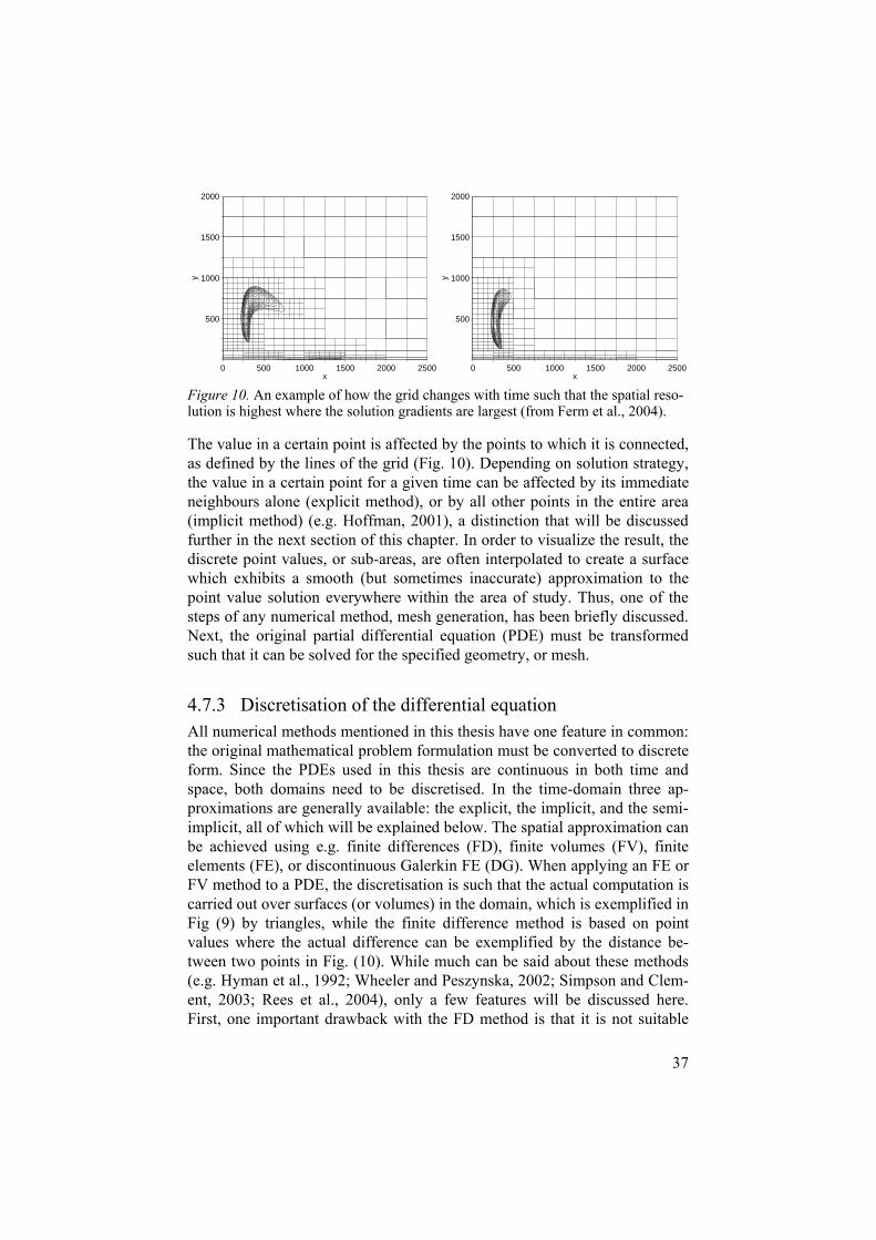
Figure 10. An example of how the grid changes with time such that the spatial reso-lution is highest where the solution gradients are largest (from Ferm et al., 2004).

The value in a certain point is affected by the points to which it is connected, as defined by the lines of the grid (Fig. 10). Depending on solution strategy, the value in a certain point for a given time can be affected by its immediate neighbours alone (explicit method), or by all other points in the entire area (implicit method) (e.g. Hoffman, 2001), a distinction that will be discussed further in the next section of this chapter. In order to visualize the result, the discrete point values, or sub-areas, are often interpolated to create a surface which exhibits a smooth (but sometimes inaccurate) approximation to the point value solution everywhere within the area of study. Thus, one of the steps of any numerical method, mesh generation, has been briefly discussed. Next, the original partial differential equation (PDE) must be transformed such that it can be solved for the specified geometry, or mesh.

4.7.3 Discretisation of the differential equation All numerical methods mentioned in this thesis have one feature in common: the original mathematical problem formulation must be converted to discrete form. Since the PDEs used in this thesis are continuous in both time and space, both domains need to be discretised. In the time-domain three ap-proximations are generally available: the explicit, the implicit, and the semi-implicit, all of which will be explained below. The spatial approximation can be achieved using e.g. finite differences (FD), finite volumes (FV), finite elements (FE), or discontinuous Galerkin FE (DG). When applying an FE or FV method to a PDE, the discretisation is such that the actual computation is carried out over surfaces (or volumes) in the domain, which is exemplified in Fig (9) by triangles, while the finite difference method is based on point values where the actual difference can be exemplified by the distance be-tween two points in Fig. (10). While much can be said about these methods (e.g. Hyman et al., 1992; Wheeler and Peszynska, 2002; Simpson and Clem-ent, 2003; Rees et al., 2004), only a few features will be discussed here. First, one important drawback with the FD method is that it is not suitable

38

for applications in several dimensions if the geometry of the problem is of non-rectangular nature. On the other hand, the FD method is easy to under-stand and implement, which can make it suitable for one-dimensional prob-lems and problems in more dimensions having simple geometries. The other methods can be applied to very complex geometries and are in that sense more general, which make them ideal for simulation of the entire road struc-ture including surroundings. The FV method and the DG method have an additional advantage in being most flexible in terms of dynamic adaptation of the mesh since they allow for something called hanging nodes (e.g. Wheeler and Peszynska, 2002). Not only geometry decides which method is most suitable to use. So is e.g. the FE method best in solving the heat trans-port equation for complex geometries under diffusion dominated conditions, while an FV method is more suitable if convection is dominant (Lötstedt, 2005, pers. com.). HYDRUS-1D (Šim nek et al., 1998) may serve as an example, where the water flow equation (a diffusion equation) is solved us-ing finite differences, while the heat transport equation (a convective-diffusion equation) is solved using finite elements even though the geometry is as simple as can be.

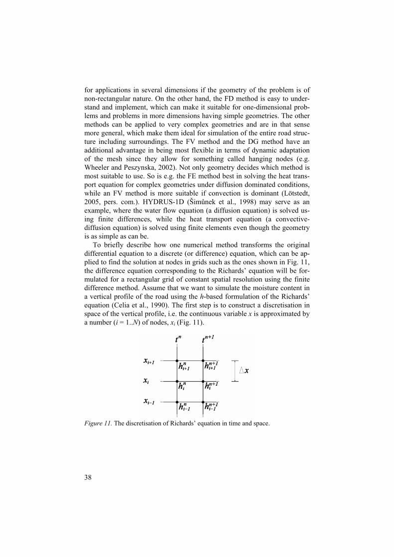
To briefly describe how one numerical method transforms the original differential equation to a discrete (or difference) equation, which can be ap-plied to find the solution at nodes in grids such as the ones shown in Fig. 11, the difference equation corresponding to the Richards’ equation will be for-mulated for a rectangular grid of constant spatial resolution using the finite difference method. Assume that we want to simulate the moisture content in a vertical profile of the road using the h-based formulation of the Richards’ equation (Celia et al., 1990). The first step is to construct a discretisation in space of the vertical profile, i.e. the continuous variable x is approximated by a number (i = 1..N) of nodes, xi (Fig. 11).

Figure 11. The discretisation of Richards’ equation in time and space.

39

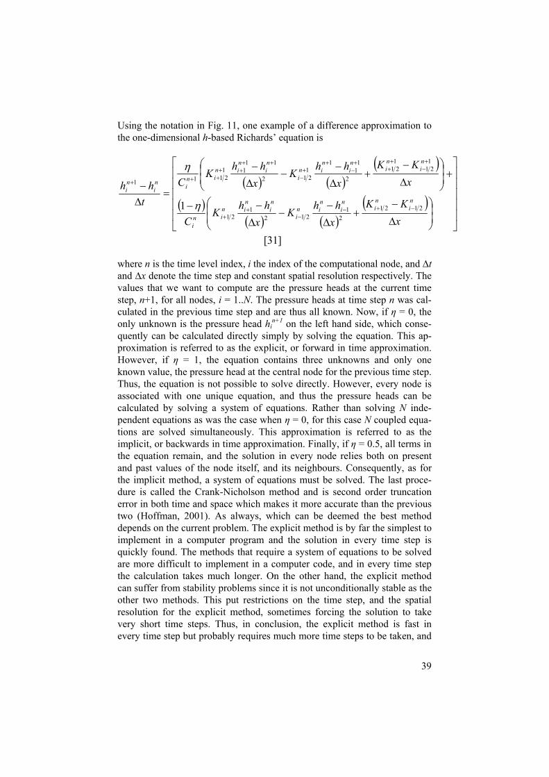
Using the notation in Fig. 11, one example of a difference approximation to the one-dimensional h-based Richards’ equation is

xKK

xhh

Kx

hhK

C

xKK

xhh

Kx

hhK

C

thh

ni

ni

ni

nin

i

ni

nin

ini

ni

ni

ni

nin

i

ni

nin

ini

ni

ni

21212

1212

121

121

121

2

11

11212

1111

2111

1

[31]

where n is the time level index, i the index of the computational node, and tand x denote the time step and constant spatial resolution respectively. The values that we want to compute are the pressure heads at the current time step, n+1, for all nodes, i = 1..N. The pressure heads at time step n was cal-culated in the previous time step and are thus all known. Now, if = 0, the only unknown is the pressure head hi

n+1 on the left hand side, which conse-quently can be calculated directly simply by solving the equation. This ap-proximation is referred to as the explicit, or forward in time approximation. However, if = 1, the equation contains three unknowns and only one known value, the pressure head at the central node for the previous time step. Thus, the equation is not possible to solve directly. However, every node is associated with one unique equation, and thus the pressure heads can be calculated by solving a system of equations. Rather than solving N inde-pendent equations as was the case when = 0, for this case N coupled equa-tions are solved simultaneously. This approximation is referred to as the implicit, or backwards in time approximation. Finally, if = 0.5, all terms in the equation remain, and the solution in every node relies both on present and past values of the node itself, and its neighbours. Consequently, as for the implicit method, a system of equations must be solved. The last proce-dure is called the Crank-Nicholson method and is second order truncation error in both time and space which makes it more accurate than the previous two (Hoffman, 2001). As always, which can be deemed the best method depends on the current problem. The explicit method is by far the simplest to implement in a computer program and the solution in every time step is quickly found. The methods that require a system of equations to be solved are more difficult to implement in a computer code, and in every time step the calculation takes much longer. On the other hand, the explicit method can suffer from stability problems since it is not unconditionally stable as the other two methods. This put restrictions on the time step, and the spatial resolution for the explicit method, sometimes forcing the solution to take very short time steps. Thus, in conclusion, the explicit method is fast in every time step but probably requires much more time steps to be taken, and

40

can thus enforce serious practical restrictions on how fine resolution can be used which in turn can affect the accuracy of the solution. To solve a system of equations such as the one outlined for the implicit case above, may be very time consuming and many methods have been developed over the years. In papers I-III, the computer programs HYDRUS-1D or HYDRUS-2D was used, and those codes utilize three methods depending on the struc-ture of the equation system matrix, which may vary according to model op-tions. The methods used are Gaussian elimination, preconditioned conjugate gradient method, or the preconditioned conjugate gradient method squared (for solute transport). For details, see the HYDRUS-2D report (Šim nek et al., 1999). The HYDRUS programs use the fully implicit formulation when solving the heat and water transport equations, while the solute transport equation solution enables more options – including the Crank-Nicholson method.

An additional complication inherent in the Richards’ equation emerges in Eq. [31] when 0. The unsaturated hydraulic conductivity, KLh, is a func-tion of h, the solution itself, and thus an iterative method must be used to solve the equation system. As a result, we were forced to develop the nu-merical solution for freezing/thawing problems presented in paper I, which will be reviewed in the next chapter.

41

5 Freezing simulation of a column experiment (paper I)

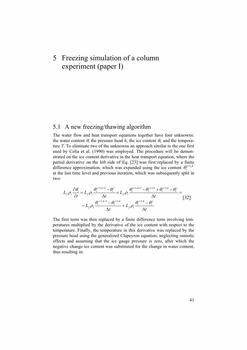
5.1 A new freezing/thawing algorithmThe water flow and heat transport equations together have four unknowns: the water content , the pressure head h, the ice content i, and the tempera-ture T. To eliminate two of the unknowns an approach similar to the one first used by Celia et al. (1990) was employed. The procedure will be demon-strated on the ice content derivative in the heat transport equation, where the partial derivative on the left side of Eq. [23] was first replaced by a finite difference approximation, which was expanded using the ice content 1,j k

iat the last time level and previous iteration, which was subsequently split in two:

1, 1 1, 1 1, 1,

1, 1 1, 1,

j k j j k j k j k ji i i i i i i

f i f i f i

j k j k j k ji i i i

f i f i

L L Lt t t

L Lt t

[32]

The first term was then replaced by a finite difference term involving tem-peratures multiplied by the derivative of the ice content with respect to the temperature. Finally, the temperature in this derivative was replaced by the pressure head using the generalized Clapeyron equation, neglecting osmotic effects and assuming that the ice gauge pressure is zero, after which the negative change ice content was substituted for the change in water content, thus resulting in:

42

tTT

dhd

gTL

tTT

dTdL

tL

kjkjkj

if

kjkjkji

if

kji

kji

if

,11,1,12

,11,1,1,11,1

. [33]

Consequently, the only unknown in Eqs. [32] and [33] is the temperature T j+1,k+1 at the new time level and the last iteration, while all other variables are known from previous calculations and can be incorporated into the right hand side of Eq. [23]. The temperature is subsequently used in the general-ized Clapeyron equation to calculate the liquid water content, which concur-rently render the ice content.

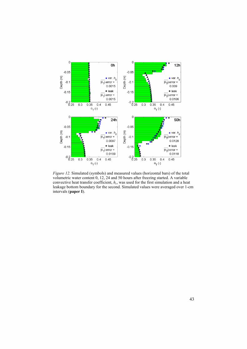
5.2 Validation of the numerical method In order to see how well the numerical solution functioned, measured surface temperatures were used to investigate the stability of the algorithm, which proved to work mostly well even though the solution progressed slowly dur-ing thawing. The code was furthermore validated using laboratory data where it again seemed to provide reasonable results (Fig. 12). Notice that the code simulates the significant freezing induced flow of water towards the freezing front well, providing an example illustration of the effect of the capillary sink mechanism mentioned in the freezing and thawing chapter. Still, it would be useful with additional validations using field data, prefera-bly measured in a Swedish road during at least one season. The two-dimensional code, which is an extension of the one-dimensional code de-scribed in this chapter, remains to be compared with either laboratory or field data.

43

Figure 12. Simulated (symbols) and measured values (horizontal bars) of the total volumetric water content 0, 12, 24 and 50 hours after freezing started. A variable convective heat transfer coefficient, hc, was used for the first simulation and a heat leakage bottom boundary for the second. Simulated values were averaged over 1-cm intervals (paper I).

44

6 Uncertainty analysis of the freezing module of the numerical model (paper II)

The numerical solution presented in paper I was new and it was thus impor-tant to investigate the degree of influence exerted on the solution by various parameters. The first evaluation was based on a Monte Carlo simulation of the laboratory freezing experiment described in paper I. In the problem formulation and succeeding analysis, the first principles of the Generalized Likelihood Uncertainty Estimation (GLUE) were used (Beven and Binley, 1992), e.g. we acknowledged the possibility of equifinality and the possible lack of an optimal parameter set. Seven parameters were included in the simulation during which 30,000 parameter sets were generated and used as input in the simulations (paper II). In order to evaluate each simulation, the simulated total water content (liquid + ice) in the cylinder was compared with the measured data using the efficiency as objective function (Nash and Sutcliffe, 1970; paper II). In GLUE, the objective function is usually re-ferred to as the likelihood function (Beven, 1993). Following the ideas of GLUE, the hydraulic parameters were sampled from log-normal probability distributions based on information from ROSETTA (Schaap et al., 2001), while the less investigated parameters were sampled from more arbitrarily chosen uniform distributions. The simulations that obtained efficiency values larger than zero were considered behavioural and formed the basis for the preceding analysis. The results were visualised by means of scatter plots (paper II), and normalized cumulative efficiency distributions (NCED) (Fig. 13).

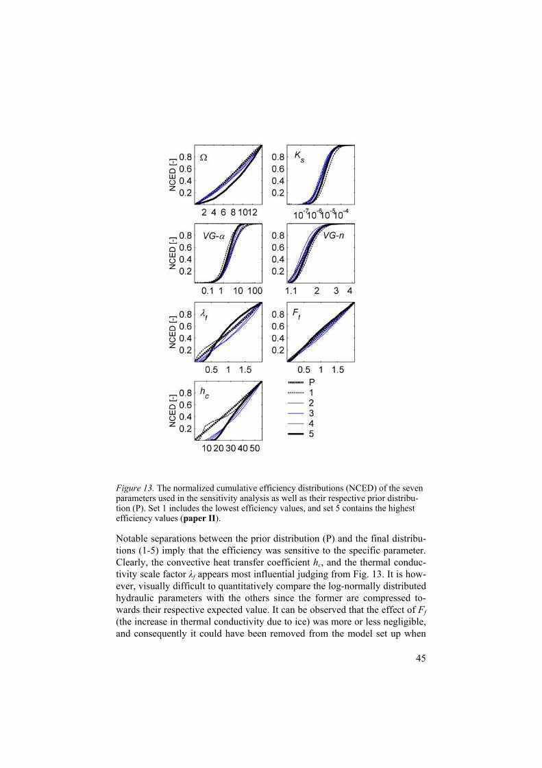
45

Figure 13. The normalized cumulative efficiency distributions (NCED) of the seven parameters used in the sensitivity analysis as well as their respective prior distribu-tion (P). Set 1 includes the lowest efficiency values, and set 5 contains the highest efficiency values (paper II).

Notable separations between the prior distribution (P) and the final distribu-tions (1-5) imply that the efficiency was sensitive to the specific parameter. Clearly, the convective heat transfer coefficient hc, and the thermal conduc-tivity scale factor f appears most influential judging from Fig. 13. It is how-ever, visually difficult to quantitatively compare the log-normally distributed hydraulic parameters with the others since the former are compressed to-wards their respective expected value. It can be observed that the effect of Ff(the increase in thermal conductivity due to ice) was more or less negligible, and consequently it could have been removed from the model set up when

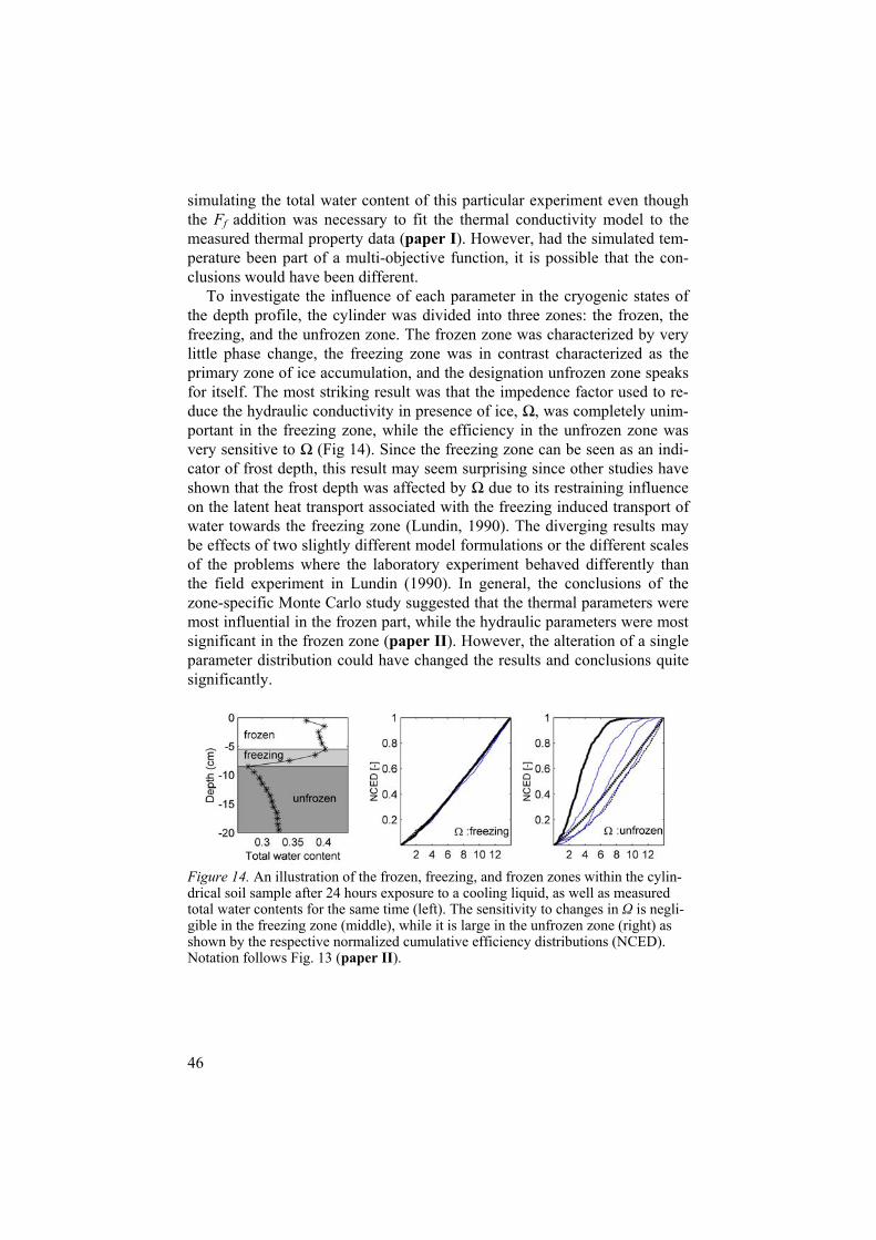
46

simulating the total water content of this particular experiment even though the Ff addition was necessary to fit the thermal conductivity model to the measured thermal property data (paper I). However, had the simulated tem-perature been part of a multi-objective function, it is possible that the con-clusions would have been different.

To investigate the influence of each parameter in the cryogenic states of the depth profile, the cylinder was divided into three zones: the frozen, the freezing, and the unfrozen zone. The frozen zone was characterized by very little phase change, the freezing zone was in contrast characterized as the primary zone of ice accumulation, and the designation unfrozen zone speaks for itself. The most striking result was that the impedence factor used to re-duce the hydraulic conductivity in presence of ice, , was completely unim-portant in the freezing zone, while the efficiency in the unfrozen zone was very sensitive to (Fig 14). Since the freezing zone can be seen as an indi-cator of frost depth, this result may seem surprising since other studies have shown that the frost depth was affected by due to its restraining influence on the latent heat transport associated with the freezing induced transport of water towards the freezing zone (Lundin, 1990). The diverging results may be effects of two slightly different model formulations or the different scales of the problems where the laboratory experiment behaved differently than the field experiment in Lundin (1990). In general, the conclusions of the zone-specific Monte Carlo study suggested that the thermal parameters were most influential in the frozen part, while the hydraulic parameters were most significant in the frozen zone (paper II). However, the alteration of a single parameter distribution could have changed the results and conclusions quite significantly.

Figure 14. An illustration of the frozen, freezing, and frozen zones within the cylin-drical soil sample after 24 hours exposure to a cooling liquid, as well as measured total water contents for the same time (left). The sensitivity to changes in is negli-gible in the freezing zone (middle), while it is large in the unfrozen zone (right) as shown by the respective normalized cumulative efficiency distributions (NCED). Notation follows Fig. 13 (paper II).

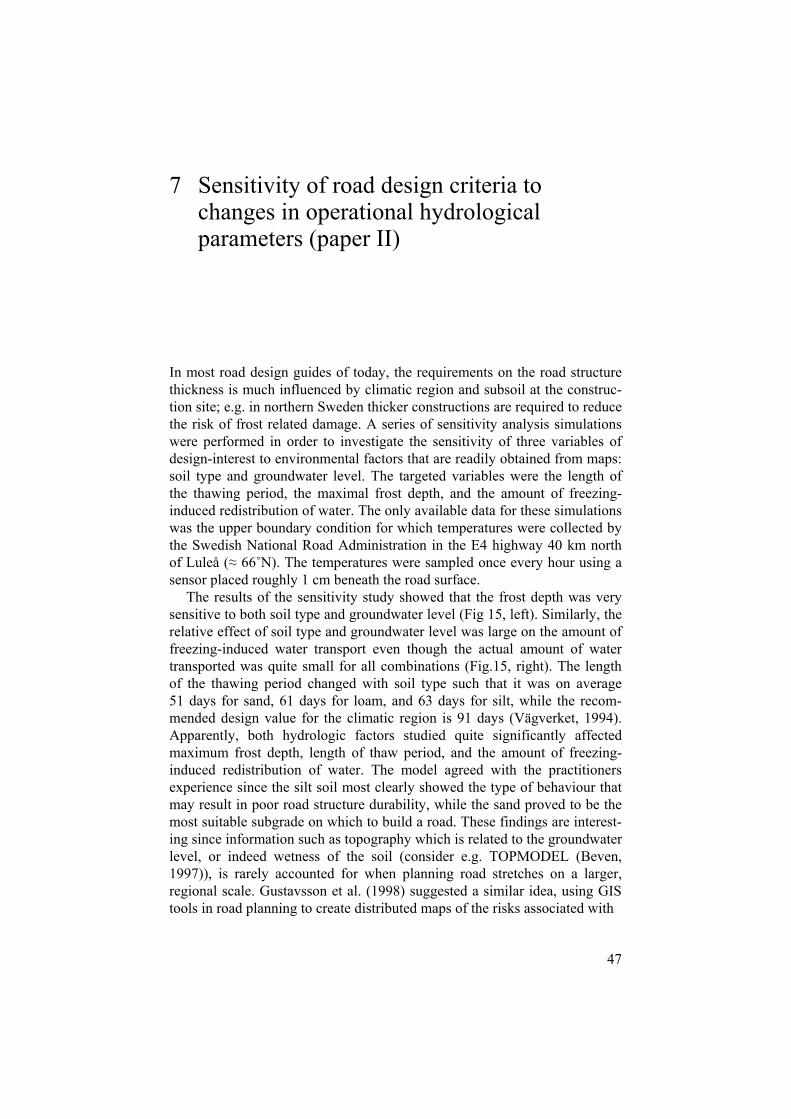
47

7 Sensitivity of road design criteria to changes in operational hydrological parameters (paper II)

In most road design guides of today, the requirements on the road structure thickness is much influenced by climatic region and subsoil at the construc-tion site; e.g. in northern Sweden thicker constructions are required to reduce the risk of frost related damage. A series of sensitivity analysis simulations were performed in order to investigate the sensitivity of three variables of design-interest to environmental factors that are readily obtained from maps: soil type and groundwater level. The targeted variables were the length of the thawing period, the maximal frost depth, and the amount of freezing-induced redistribution of water. The only available data for these simulations was the upper boundary condition for which temperatures were collected by the Swedish National Road Administration in the E4 highway 40 km north of Luleå ( 66˚N). The temperatures were sampled once every hour using a sensor placed roughly 1 cm beneath the road surface.

The results of the sensitivity study showed that the frost depth was very sensitive to both soil type and groundwater level (Fig 15, left). Similarly, the relative effect of soil type and groundwater level was large on the amount of freezing-induced water transport even though the actual amount of water transported was quite small for all combinations (Fig.15, right). The length of the thawing period changed with soil type such that it was on average 51 days for sand, 61 days for loam, and 63 days for silt, while the recom-mended design value for the climatic region is 91 days (Vägverket, 1994). Apparently, both hydrologic factors studied quite significantly affected maximum frost depth, length of thaw period, and the amount of freezing-induced redistribution of water. The model agreed with the practitioners experience since the silt soil most clearly showed the type of behaviour that may result in poor road structure durability, while the sand proved to be the most suitable subgrade on which to build a road. These findings are interest-ing since information such as topography which is related to the groundwater level, or indeed wetness of the soil (consider e.g. TOPMODEL (Beven, 1997)), is rarely accounted for when planning road stretches on a larger, regional scale. Gustavsson et al. (1998) suggested a similar idea, using GIS tools in road planning to create distributed maps of the risks associated with

48

Figure 15. Left: The maximum frost depth beneath the road surface for different groundwater depths beneath the same surface and different subgrades (sand, loam, silt). Right: The simulated maximum increase in water content, depth-averaged (0.99 to 4.2 m), as compared to the initial water content for different subgrades (sand, loam, silt). The increase in water content at the respective temporal maxi-mum occurs at, or near, the end of the thawing period (paper II).

low surface temperatures (icy, slippery surfaces) based on climatological factors. As a concluding remark, the results obtained when using a numerical simulation model that utilises high-resolution meteorological data as upper boundary condition are very different from the tabulated default values used to estimate e.g. piecewise constant elastic modulus values. Undoubtedly, the elastic modulus of any road structure varies continuously, and in particular for poor quality roads it is widely recognized that “damage caused by just a few heavy vehicles on a low volume road during critical thaw-weakened conditions … can exceed the damage caused by design traffic the entire re-mainder of the year” (Kestler et al., 2005). To capture such extreme behav-iour, simulation models are necessary. The other major advantage with nu-merical models as the one used here, which are physically based, is the pos-sibility to use them exactly as was done in this study; i.e. to investigate the impact of different designs, or different environmental conditions, on state variables that affect the predicted life span. However, it would be necessary to validate the model for a large number of roads spanning different climatic regions and road structures, before this or any similar model could be used in practice. Undoubtedly, for practical reasons some sort of automatic calibra-tion algorithm would be beneficial to estimate e.g. the thermal and hydraulic parameters used to compute the respective properties.

49

8 Effect of rainfall and fracture zone conductivity on the subsurface flow pattern (paper III)

In paper III, the unsaturated hydraulic conductivity of the asphalt layer was assumed to decrease with saturation in the same way as a sandy soil. An example showing the simulated water content distribution in a road follow-ing a rainfall event as affected by the combined effects of surface runoff and infiltration through fractures in the paving is showed in Fig. 17. Notice that the fracture zone captures most, if not all, of the upstream surface runoff for the light rainfall event. The heavier rainfall causes a significantly larger infil-tration in the road shoulder since the infiltration capacity of the fracture zone, or the base layer beneath it, was exceeded. As a consequence, a larger fraction of the total surface runoff reached the road shoulder, and the region of the road side where both rainfall and surface runoff infiltrated was con-siderably expanded laterally. This result is qualitatively supported by the findings of Flyhammar and Bendz (2003) who measured concentrations of various solutes in the shoulder and beneath the asphalt cover in a Swedish road partly built with alternative materials, generated from waste and residu-als. These materials contained plenty of solutes, and the leaching pattern is similar to the simulated water flow pattern, although the leaching patterns exhibited a large variability between solutes.

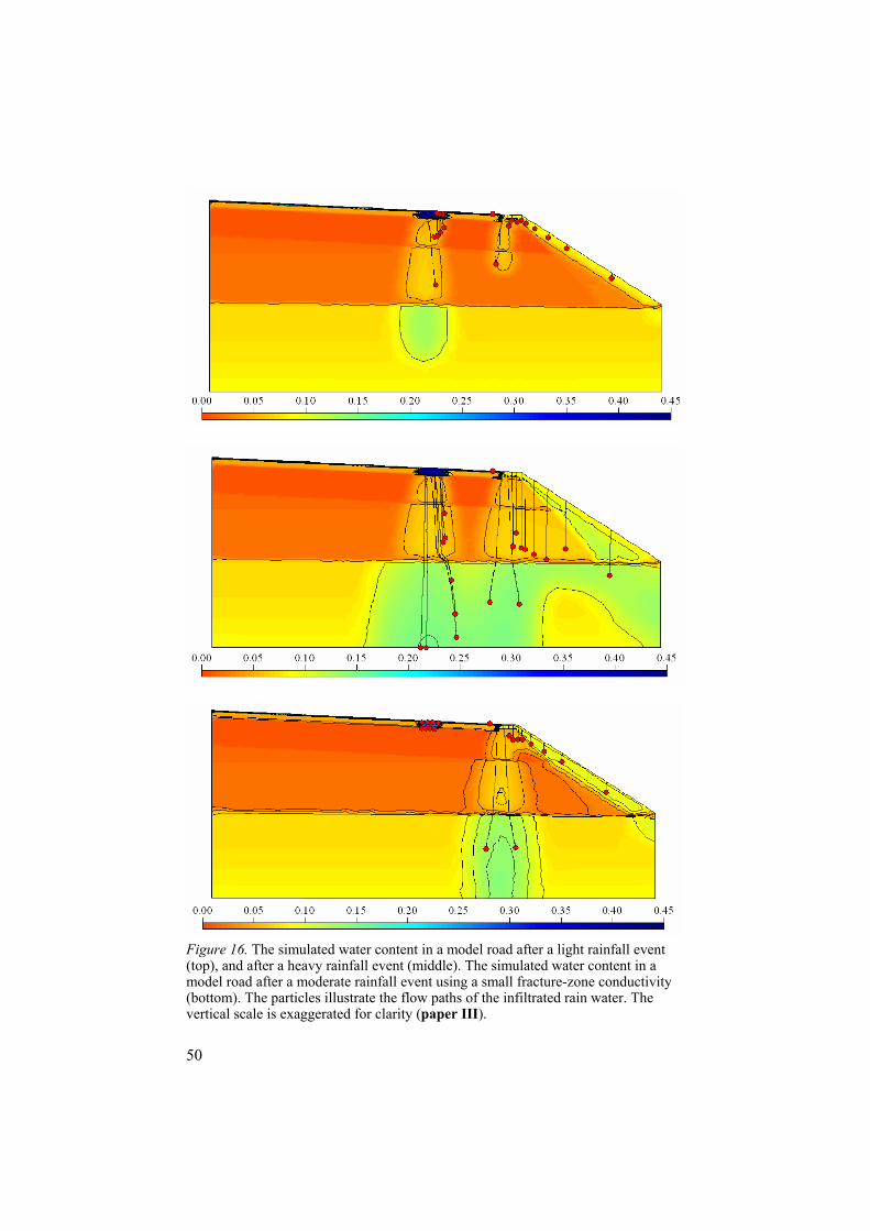
50

Figure 16. The simulated water content in a model road after a light rainfall event (top), and after a heavy rainfall event (middle). The simulated water content in a model road after a moderate rainfall event using a small fracture-zone conductivity (bottom). The particles illustrate the flow paths of the infiltrated rain water. The vertical scale is exaggerated for clarity (paper III).

51

9 Application of TDR and WCR in road materials (paper IV)

9.1 Dielectric models Topp et al. (1980) published a famous paper on TDR that contributed greatly in making TDR a widespread technique, and since then many equations have been proposed to interpret the output of the TDR in terms of volumetric wa-ter content. However, the very first step in the interpretation of the output signal from the TDR is to determine the travel time along the rods, which can be done in several ways (e.g. Klemunes, 1998). Following this, the ap-parent dielectric number is calculated from the travel time (e.g. Topp et al., 1980). The equations that relate the apparent dielectric number to water con-tent can be divided into two groups: empirical or mixing models. The em-pirical models do not have a physical base, and simply consist of a regres-sion equation relating the apparent dielectric number to water content. In some cases, empirical equations have been modified to include physical parameters such as bulk density, thus making them semi-empirical (Jacobsen and Schjønning, 1995). The mixing models are based on estimating the di-electric number of the material taking the fractions of solids, water, air, and sometimes bound water, and their respective dielectric number into account. Since the apparent dielectric number was determined by the measured travel time, the water content can be solved for. Because the mixing models have a physical base, they have a larger potential for use in a wide range of materi-als.

9.2 A function yielding the dielectric number from WCR output

The output of the WCR sensor is not a trace from which the travel time can be determined as is the case for the TDR. Instead, the trace is translated by the electronics embedded in the probe head directly to a period (Bilskie, 1997). The manufacturer of the probe (Campbell Scientific, 2003) suggests a couple of empirical equations relating the period to water content, where the choice of equation depends on range of water content and concentration of solutes in the pore water. Obviously, it would be beneficial if the equations

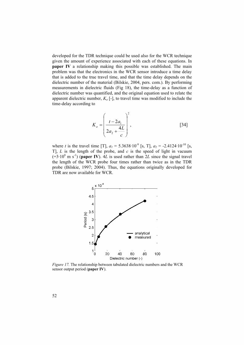
52

developed for the TDR technique could be used also for the WCR technique given the amount of experience associated with each of these equations. In paper IV a relationship making this possible was established. The main problem was that the electronics in the WCR sensor introduce a time delay that is added to the true travel time, and that the time delay depends on the dielectric number of the material (Bilskie, 2004, pers. com.). By performing measurements in dielectric fluids (Fig 18), the time-delay as a function of dielectric number was quantified, and the original equation used to relate the apparent dielectric number, Ka [-], to travel time was modified to include the time-delay according to

2

2

1

42

2

cLa

atKa , [34]

where t is the travel time [T], a1 = 5.3638·10-9 [s, T], a2 = -2.4124·10-10 [s, T], L is the length of the probe, and c is the speed of light in vacuum (=3·108 m s-1) (paper IV). 4L is used rather than 2L since the signal travel the length of the WCR probe four times rather than twice as in the TDR probe (Bilskie, 1997; 2004). Thus, the equations originally developed for TDR are now available for WCR.

Figure 17. The relationship between tabulated dielectric numbers and the WCR sensor output period (paper IV).

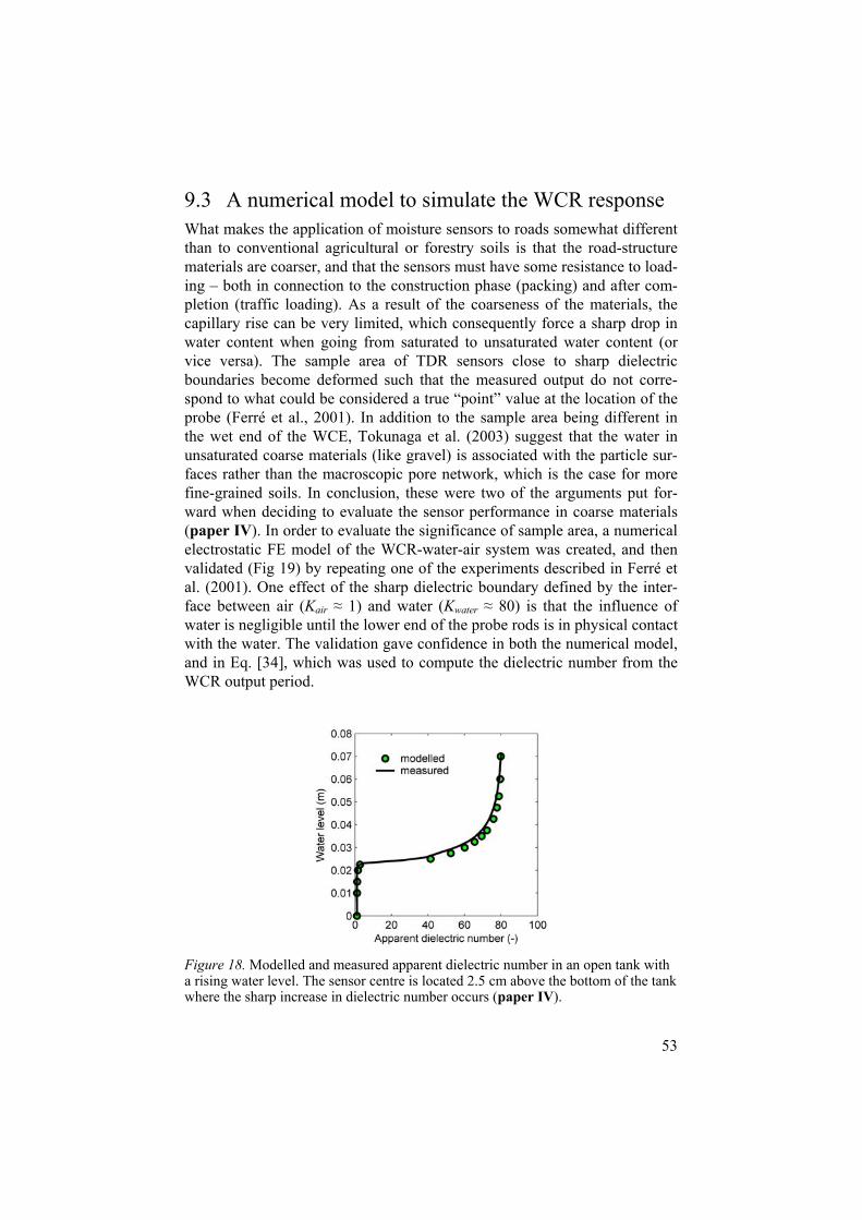
53

9.3 A numerical model to simulate the WCR response What makes the application of moisture sensors to roads somewhat different than to conventional agricultural or forestry soils is that the road-structure materials are coarser, and that the sensors must have some resistance to load-ing – both in connection to the construction phase (packing) and after com-pletion (traffic loading). As a result of the coarseness of the materials, the capillary rise can be very limited, which consequently force a sharp drop in water content when going from saturated to unsaturated water content (or vice versa). The sample area of TDR sensors close to sharp dielectric boundaries become deformed such that the measured output do not corre-spond to what could be considered a true “point” value at the location of the probe (Ferré et al., 2001). In addition to the sample area being different in the wet end of the WCE, Tokunaga et al. (2003) suggest that the water in unsaturated coarse materials (like gravel) is associated with the particle sur-faces rather than the macroscopic pore network, which is the case for more fine-grained soils. In conclusion, these were two of the arguments put for-ward when deciding to evaluate the sensor performance in coarse materials (paper IV). In order to evaluate the significance of sample area, a numerical electrostatic FE model of the WCR-water-air system was created, and then validated (Fig 19) by repeating one of the experiments described in Ferré et al. (2001). One effect of the sharp dielectric boundary defined by the inter-face between air (Kair 1) and water (Kwater 80) is that the influence of water is negligible until the lower end of the probe rods is in physical contact with the water. The validation gave confidence in both the numerical model, and in Eq. [34], which was used to compute the dielectric number from the WCR output period.

Figure 18. Modelled and measured apparent dielectric number in an open tank with a rising water level. The sensor centre is located 2.5 cm above the bottom of the tank where the sharp increase in dielectric number occurs (paper IV).

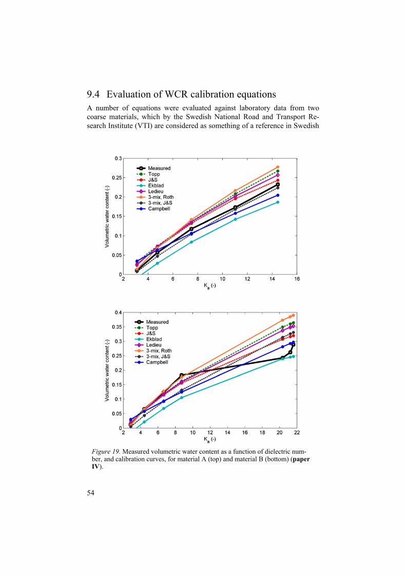
54

9.4 Evaluation of WCR calibration equations A number of equations were evaluated against laboratory data from two coarse materials, which by the Swedish National Road and Transport Re-search Institute (VTI) are considered as something of a reference in Swedish

Figure 19. Measured volumetric water content as a function of dielectric num-ber, and calibration curves, for material A (top) and material B (bottom) (paper IV).

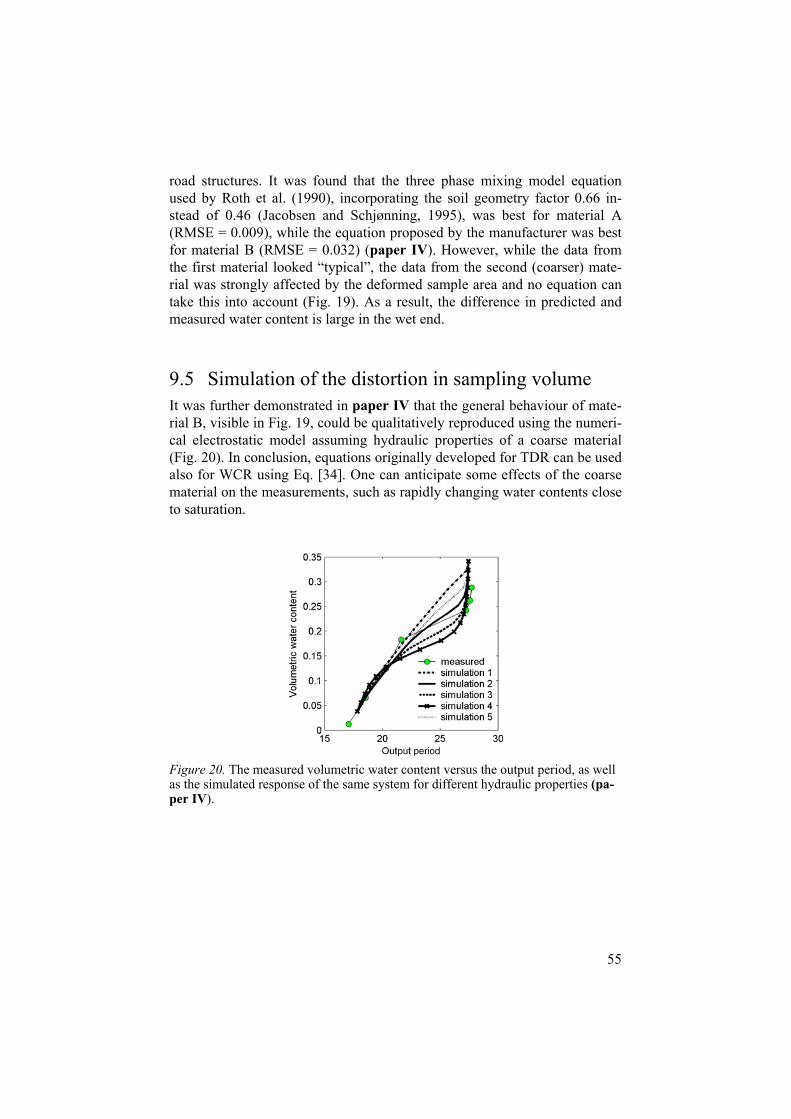
55

road structures. It was found that the three phase mixing model equation used by Roth et al. (1990), incorporating the soil geometry factor 0.66 in-stead of 0.46 (Jacobsen and Schjønning, 1995), was best for material A (RMSE = 0.009), while the equation proposed by the manufacturer was best for material B (RMSE = 0.032) (paper IV). However, while the data from the first material looked “typical”, the data from the second (coarser) mate-rial was strongly affected by the deformed sample area and no equation can take this into account (Fig. 19). As a result, the difference in predicted and measured water content is large in the wet end.

9.5 Simulation of the distortion in sampling volume It was further demonstrated in paper IV that the general behaviour of mate-rial B, visible in Fig. 19, could be qualitatively reproduced using the numeri-cal electrostatic model assuming hydraulic properties of a coarse material (Fig. 20). In conclusion, equations originally developed for TDR can be used also for WCR using Eq. [34]. One can anticipate some effects of the coarse material on the measurements, such as rapidly changing water contents close to saturation.

Figure 20. The measured volumetric water content versus the output period, as well as the simulated response of the same system for different hydraulic properties (pa-per IV).

56

10 Conclusions

1. Soil physical, hydrological, and hydraulic models provided a means of simulating the coupled transport of water and heat in and on the road struc-ture.

2. A numerical algorithm accounting for freezing and thawing processes was developed and successfully incorporated together with a new thermal con-ductivity function into a fully implicit numerical model describing the cou-pled water and heat transport in one and two dimensions.

3. Easily available information such as soil type and groundwater level strongly influenced the maximum frost depth, the length of the thawing pe-riod, and the amount of freezing-induced water flow.

4. The addition of a surface runoff algorithm in combination with the con-cept of equivalent porous media enabled two-dimensional simulations of rainfall infiltration into the road structure, which qualitatively agreed with field observations.

5. An equation was developed that enables classical TDR equations to be used for WCR sensors.

6. The WCR sampling volume can be distorted in coarse road materials due to limited capillary rise.

7. Measurements are often used to validate or reject numerical models since measurements are often considered to represent the truth. However, it was demonstrated in this thesis that numerical models can also be used to im-prove the interpretation and explanation of measurements. It can be con-cluded that both measurements and numerical computations benefit from each other, and that the two disciplines will become more intimately linked in the future given the advent of new numerical multi-physics tools.

57

11 Future developments and recommendations

11.1 Research phase It’s about time that the unresolved problem of freezing is solved, by somehow merging the two schools into one. Perhaps a first step could be to introduce an empirical relationship between the ice and water pressures as a function of ice content. Today, frost heave in hydrodynamic models is generally assumed to commence e.g. when the total water content ex-ceeds porosity, but often without considering that a continuing tempera-ture drop must be distributed on both ice and capillary pressure, thus this change would reduce the freezing-induced redistribution of water. Is it important to consider effects of dynamic loading on water flow? As mentioned in the thesis, measurements beneath concrete road structures have shown that the envelope potential, as governed by traffic load, gave raise to significant water flow. It would be interesting to investigate if this can happen also in flexible pavements, and what the effect would be. Discrete particle models, which operate on particle-size distribution and degree of packing, could potentially be used to approximate hydraulic and thermal property functions. It appears that in dealing with coarse materials of the type used in road structures, processes controlled by particle surfaces are more important than for soils. Such processes include frost heave and film flow where water is transported in a thin layer close to the surface even if the pore is empty. A related question is whether the water transport is governed by Richards’ equation in very coarse materials. What are the alternatives? A further development of the model used in the thesis to include snow and plough routines, and effects of solutes on freezing would be a tempt-ing next step. According to Therrien (2004, pers. com.), the salinity of pore water close to roads can be more than enough to generate density driven flow, and thus algorithms describing this could prove useful. In addition, dynamic adaptive meshing should be considered, both as a means of improving simulation quality, and as a way to improve user-friendliness.In the best of worlds, the ultimate road simulation model should be of multi-physical nature. I.e., the model should comprise geo-mechanics,

58

density-driven flow, multi-phase flow, frost heave, snow pack, solute transport, geochemistry, and reactive transport. Couplings between water flow models and reactive transport models have evolved the last few years [PHREEQC (Parkhurst and Apello, 1999), HYDRUS-PHREEQC (Jacques and Simunek, 2005), and CoupModel-Visual MINTEQ (Gustafsson, 2005, pers. com.)] in response to the needs of society. These models are being increasingly used when studying leaching from secon-dary materials used in road structures, parking lots, air strips and similar infrastructure. It is important to develop multi-physics models, even though there is a risk that only a limited number of people possess the vast knowledge needed to use them correctly.

11.2 Application phase Establish a measurement site in order to make possible an evaluation, and if possible validation, of the hydrodynamic models of freezing presented in this thesis, or improvements of the same. Concurrently, water content, temperature and conductivity should be monitored during several seasons to provide the complete picture at least for one site. Investigate if it is possible to evaluate thermal and hydraulic properties in road materials using inverse modelling on the VViS stations of Vägverket (SNRA). The nature of the coupling between temperature, water, and ice content suggests that might be (e.g. Bittelli et al., 2003). Use distributed models (or GIS-tools) in the planning process of new road stretches to predict where problems associated with wetness are likely to occur.Models such as the one used in this thesis can provide useful insights into the mechanisms that decide when spring thaw occurs and predict the se-verity for a given location through short-term forecasts. In this context, they could be useful in making decisions on e.g. spring load restrictions on low volume roads.

59

12 Acknowledgements

First I would like to thank my main supervisor Lars-Christer Lundin and Sven Halldin for employing me almost five years ago. It is fair to say that was a step of fundamental importance for this thesis project. Some qualities of L-C which I have found particularly valuable are that he is flexible and positive (problems can always be solved), as well as smart and experienced in the worlds of science, writing, and economics. I feel that we are similar in having a quite easy-going attitude towards most problems. Unfortunately he has sometimes suffered from my tendencies to deliver VERY close to dead-lines, and as an example I will soon send him this thesis for proof reading even though it is Sunday…

The other supervisors have been Per-Erik Jansson at the Dept. of Land and Water Resources Engineering at the Royal Institute of Technology in Stockholm, and Åke Hermansson at the Swedish National Road and Trans-port Research Institute in Linköping. It is always a good idea to listen care-fully to what PEJ has to say because he is one of those persons who always appear to be right in the end. And like L-C, he has the ability to condense a lot of bla-ha, bla-ha to very short conclusions. I hope that is a quality that comes with experience... Åke obviously brought in knowledge and experi-ence about roads which I could hardly have gained otherwise. I feel now that it is a pity I did not spend time in the laboratories of VTI, both with Åke and others, I would have learned a lot. At least, the balance from VTI finally enabled me to do WCR measurements in road materials.

Jirka Šim nek, now at the Department of Environmental Sciences at the University of California in Riverside has been hugely influential on this pro-ject. I counted the number of e-mails in my mailbox (i.e. excluding deleted ones) and found that we had exchanged more than 450 e-mails over ap-proximately three years. Those figures speak for themselves and I deeply appreciate the co-operation that has worked well even though there is a nine hours time difference between California and Uppsala. Also, I know after being at the Salinity Lab that e-mails pop up all the time on Jirkas computer screen so I don’t really understand how he manages to do all the things he does.

I am grateful to Per Lötstedt at the Dept. of Information Technology at Uppsala University for checking and correcting parts of the writings on nu-merical analysis in the thesis.

60

In many ways the people at the department have been most important in the long process of PhD studies since they have contributed to the excellent so-cial environment we have at LUVA within our department. A few persons have been more involved in my everyday working life than others. Fredrik Wetterhall, my room mate, with whom I have spent many late evenings at the department working. He is presently in Germany for a number of weeks, and it is really not as fun working when there is no one to discuss the best music track of the week with or something equally important. I have had many fruitful scientific discussions with Niclas Bockgård, Johan Öhman, Fritjof Fagerlund, and Allan Rodhe. Obviously they are not only smashing scientists, but also sociable. Tomas Nord has kept everything up and running as far as computers are concerned; a task that has become increasingly de-manding in recent years. No equipment has been more important for me than my computers so I appreciate your help Tomas. I furthermore appreciate the kind assistance provided by Taher Mazloomian and Anna Callerholm at Geotryckeriet over the years. Finally, I would like to thank the lunch group for all the entertaining lunch breaks.

I am grateful to Vägverket (SNRA) for financing this project. In particular I would like to mention the enthusiastic Hans Wirstam who was the first supervisor of this project, and my recent contacts at Vägverket; Klas Her-melin and Torbjörn Svensson. I further acknowledge the financial support by Hans Werthén-fonden and Vägverket for generously enabling me to work in Riverside in 2002. In this context I would like to thank Rien van Genuchten at the Salinity Lab for providing me with a room including computer; Theijs Kelleners for renting me his apartment; Marcel Schaap for lending me his bike; David Robinson, Inma Lebron, and Heinrich for taking me on excur-sions and inviting me to dinners during weekends. Two other sources of financial support were the scholarships Rektors Wallenbergsmedel that al-lowed me to attend a conference in New Hampshire, USA, last spring which brought me into contact with alternative materials in roads; and Liljewalchs stipendiefond that provided me with the money needed to attend the best, and most inspirational conference ever in Oxford, G.B., last summer.

Having finished the thesis, I look forward to the spring; relaxing; watch-ing ice hockey playoffs (thanks Zdeno Chara, Sheldon Souray and Martin Gerber); travelling to Australia with Ando and Janne; and much more.

Finally, and most importantly, I would like to thank family and friends. How awful and hopeless wouldn’t life have been without you? Now, instead, it is good!

61

13 Summary in Swedish

En vägs livslängd påverkas, förutom av dess konstruktion och terrängläge, av faktorer som trafikmängd och andelen tung trafik, men också av klimato-logiskt och markfysikaliskt styrda processer såsom tjälning och tjällossning. Exempelvis kan en väg bära stora laster då den är frusen, men förstörs lätt om den innehåller för mycket vatten vilket kan vara fallet under tjällossning-en. I fuktiga terränglägen blir också vägens dräneringsegenskaper avgörande för dess funktion. Med tanke på kostnaderna för vägbyggnation och vägun-derhåll ställs ökande krav på kostnadseffektivitet. Som exempel kan nämnas att Vägverket innevarande år (2005) av Näringsdepartementet fått 1,2 mil-jarder kronor öronmärkta för bärighetsförbättrande åtgärder och reparationer på vägar som skadats i samband med frysning/tjällossning. Detta är bak-grunden och motivet till att det är viktigt att inkludera vatten- och värme-transportprocesser i analysen när vägen konstrueras, inte minst för att realis-tiskt inkludera kostnaderna för underhåll.

Det övergripande målet var att utveckla en numerisk modell som lämpar sig för att beräkna vatten- och värmeflöden i en väg och dess närmaste om-givningar i ett kallt klimat. Dessutom var ett mål att utvärdera metoder för att mäta vattenhalten i den typ av grova material som används i vägbyggna-tioner.

I arbetet mot det övergripande målet utvecklades en algoritm för att in-kludera fasomvandlingen mellan vatten och is i en befintlig en- och tvådi-mensionell, iterativ, implicit modellkod för simulering av vatten-, värme- och ämnestransport under omättade och mättade förhållanden (HYDRUS-1D/2D). Hur värdet på olika modellparametrar påverkade resultatet under-söktes genom Monte Carloanalys där den simulerade totala vattenhalten (flytande vatten + is) jämfördes med mätningar gjorda på cylindrar som fru-sits i ett laboratorieförsök av Mizoguchi (1990). Hur modellerade resultat såsom maximalt tjäldjup, tjälperiodens längd och frysningsgenererade vat-tenflöden påverkades av variationer i lättillgängliga data som grundvatten-djup och jordart undersöktes genom känslighetsanalys. En programrutin för simulering av ytavrinning och användandet av konceptet ekvivalent poröst medium implementerades för att möjliggöra simuleringar av vägtvärsnitt med sprickor i ytan. Simulerade partiklar användes för att visualisera flödes-banorna inuti vägkroppen.

En tank i plexiglas byggdes för att utvärdera vattenhaltsreflektometrar i laboratoriet. Tanken fylldes med två olika vägbyggnadsmaterial varefter

62

vatten fylldes på i intervaller. Mätvärdena kunde sedan jämföras med den kända vattenhalten och ett antal kalibreringsfunktioner utvärderades. En numerisk elektrostatisk modell konstruerades för att simulera hur givarens respons påverkades av vattenhalten hos materialet i behållaren.

I samband med utvecklandet av den nya programrutinen för simulering av frys/tiningsförloppet blev det nödvändigt att ta fram en ny funktion för vär-meledningsförmågan som inkluderade ett beroende av ishalt likväl som vat-tenhalt. Den nya numeriska lösningen visade sig vara stabil även då uppmät-ta högupplösta vägytetemperaturer användes som indata. Modellen tillämpa-des på ett laboratorieexperiment där cylindrar frystes och efterhand skivades för bestämning av den totala vattenhalten (flytande vatten + is) varvid simu-lerade data överensstämde väl med uppmätta. Från Monte Carloanalysen gick det inte att dra några slutsatser om huruvida någon parameter var onö-dig, men vissa parametrar påverkade överrensstämmelsen mellan uppmätta och simulerade värden mer än andra. Resultatet av analysen förändrades om kolumnen delades upp i tre zoner där en var frusen, en ofrusen och där den tredje innefattade tjälfronten, då det visade sig att den hydrauliska parameter som styr hur mycket motståndet mot vattenflöde ökar då vissa porer fylls med is istället för vatten var väldigt betydelsefull i den ofrusna zonen, men annars betydelselös. Känslighetsanalysen visade att det maximala tjäldjupet är starkt beroende av avståndet från markytan till grundvattenytan. När grundvattenytan höjdes från fem till tre meter under markytan minskade tjäldjupet med knappt en meter för en modellväg byggd på en sandjord och med ungefär en halv meter då den byggts på en silt- eller loamjord (bland-ning av sand, silt och lera). Tjälperiodens längd påverkades kraftigt av jord-art. Frysningsgenererade vattenflöden var störst i siltjorden och så gott som försumbar i sandjorden. De förändringar som gjordes i den två-dimensionella numeriska modellen för att kunna studera ytavrinning och infiltration genom sprickor i asfalten fungerade tillfredsställande. De simule-ringar som utfördes visade att små sprickor kan leda till stor infiltration av regnvatten genom asfalten och vidare ner i vägkroppen. Det vatten som rin-ner av vägytan infiltrerar i vägbanken och ökar på så vis infiltrationen där. Under kraftiga skyfall ökar ytavrinningen och en större del av vägslänten utsätts för ökad infiltration i takt med att regnmängderna ökar. Infiltrations-ökningens utsträckning beror på släntmaterialets, och eventuella underlig-gande materials, förmåga att leda bort vatten.

Vattenhalt i porösa material mäts ofta med en teknik som kallas time do-main reflectrometry (TDR) och bygger på att materialets dielektricitetstal mäts. För TDR-givare har ett stort antal ekvationer som beskriver sambandet mellan vattenhalten och det skenbara dielektricitetstalet presenterats under de senaste 30 åren. En ny, likartad teknik som kallas water content reflecto-metry och ger vattenhalten direkt finns tillgänglig sedan några år. Av natur-liga skäl har den ännu inte utvärderats i samma omfattning som TDR-tekniken. En ny ekvation presenterades som tar hänsyn till den tidsfördröj-

63

ning, jämfört med TDR-givarna, som WCR-givarna uppvisar. Genom detta kunde WCR-givarnas utdata transformeras från period, som är den signal som mäts, till ett skenbart dielektricitetstal så att tidigare framtagna TDR-ekvationer kan användas och utvärderas. För det ena vägmaterialet visade det sig att en ekvation använd av Roth et al. (1990), senare justerad av Ja-cobsen och Schjønning (1995), gav minst skillnad mellan uppmätt och pre-dikterad vattenhalt, medan ingen ekvation på ett rimligt sätt återgav det uppmätta förhållandet mellan skenbart dielektricitestal och vattenhalt för det andra materialet. Emellertid kunde det ovanliga utseendet, med hjälp av en numerisk simulering av hur givarens mätvolym förändrades i takt med att vatten fylldes på i tanken, visas bero på en begränsad kapillär stighöjd i det grova materialet, vilket gav upphov till effekter liknande de som tidigare observerats nära skarpa övergångar i dielektricitetstal.

Till följd av sin speciella struktur erbjuder vägar en utmaning för en mo-dellerare men genom att kombinera numeriska modeller från markfysiken, hydrologin och fluidmekaniken kunde de kopplade vatten- och värmetrans-portsprocesser som varit föremål för denna studie framgångsrikt beskrivas. Den nyutvecklade fasomvandlingsalgoritmen tillsammans med den nya ek-vationen för värmeledningsförmågan fungerade bra. Tjäldjup, längden på tjälperioden och frysningsgenererade vattenflöden påverkades kraftigt av avståndet från markytan till grundvattenytan och vilken jordart vägen byggs på. Tillägget av programrutiner för simulering av ytavrinning och konceptet att simulera sprickor med ett ekvivalent poröst medium gjorde att den nume-riska modellen är väl lämpad för simuleringar av vattenflöden i ett tvärsnitt av vägkroppen och dess omgivning. Nyligen genomförda studier av Fly-hammar och Bendz (2003) visade att mest vatten infiltrerar i närheten av asfaltskanten (beroende på ytans beskaffenhet) vilket kvalitativt överens-stämmer med de simulerade vattenströmningsfälten. En nyutvecklad ekva-tion gör att utsignalen från en WCR-givare kan transformeras så att befintli-ga TDR-ekvationer kan användas för att prediktera vattenhalt med WCR-mätningar. Givarens mätvolym kan bli deformerad i närheten av grundvat-tenytan om mätningen utförs i ett grovt material. Mätdata används ofta för att bedöma om en numerisk modell producerar användbara och korrekta resultat, men det visades också i denna studie hur numeriska modeller kan användas för att öka förståelsen för hur en givare samverkar med sin omgiv-ning, vilket underlättar tolkningen av mätdata.

64

14 References

Alberty, R.A., Silbey, R.J., 1992. Physical chemistry. John Wiley & Sons, Singa-pore.

Arya, Lalit. 2003. Personal communication. Arya, L.M., Paris, J.F., 1981. A physicoempirical model to predict the soil moisture

characteristic from particle-size distribution and bulk density data. Soil Sci. Soc. Am. J. 45:1023-1030.

Bárány, A., Yngve, S., 1994. Fysikens matematiska metoder, Exempelsamling för civilingenjörsutbildningen. Inst. f. teoretisk fysik, Uppsala universitet. (In Swe-dish).

Baumhardt, R.L., Lascano, R.J., Evett, S.R., 2000. Soil material, temperature, and salinity effects on calibration of multisensor capacitance probes. Soil Sci. Soc. Am. J., 64:1940-1946.

Bern, M., Plassmann, P., 2000. Mesh generation. In J.-R. Sack, Urrutia, J. (eds.), Handbook of Computational Geometry, Elsevier Science, January, 2000, pp 291-332.

Beven, K., 1993. Prophecy, reality and uncertainty in distributed hydrological mod-elling. Adv. Water Resour., 16:41-51.

Beven, K.J, (Ed.), 1997, Distributed Modelling in Hydrology: Applications of TOPMODEL, Wiley, Chichester.

Beven, K., Binley, A., 1992. The future of distributed models: model calibration and uncertainty prediction. Hyd. Process., 6:279-298.

Bilskie, Jim, 2004. Campbell Scientific Inc. Personal communication. Bilskie, J., 1997. Using dielectric properties to measure soil water content. Sensors

Magazine, Vol. 14. Bittelli, M., Flury, M., Campbell, G.S., 2003. A thermo-dielectric analyzer to meas-

ure the freezing and moisture characteristic of porous media, Water Resour. Res., 39, 1041, doi:10.1029/2001WR000930.

Bouma, J., 1989. Using soil survey data for quantitative land evaluation. Adv. Soil Sci. 9:177-213.

Brooks, R.H., Corey A.T. 1964. Hydraulic properties of porous media, Hydrology Paper No. 3, Colorado State University, Fort Collins, Colorado.

Burdine, N.T., 1953. Relative permeability calculations from pore size distributions data. Trans. Am. Inst. Univ. Pet. Eng. 198:71-87.

Campbell, G.S., 1985, Soil physics with BASIC, Elsevier, New York, NY. Campbell Scientific, 2003. CS616 and CS625 water content reflectometers instruc-

tion manual. Campbell Scientific, Inc. Logan, UT. Carsel, R.F., Parrish, R.S., 1988. Developing joint probability distributions of soil

water retention characteristics. Water Resour. Res. 24:755-769. Celia, M.A., E.T. Bouloutas, R.L. Zarba, 1990. A general mass-conservative nu-

merical solution for the unsaturated flow equation. Water Resour. Res. 26(7):1483-1496.

65

Chung S.-O., Horton, R., 1987. Soil heat and water flow with a partial surface mulch, Water Resour. Res., 23(12), 2175-2186.

Claesson, J., 1993. A few remarks on moisture flow potentials. Prepared for HAM-TIE Meeting in Glasgow. Dept. of Building Technology, Building Physics, Chalmers Technical University, Sweden.

Crowe, C.T., Elger, D.F., Roberson, J.A., 2001. Engineering fluid mechanics. 7th

edition. John Wiley & Sons, New York City, New York. Dean, T.J., Bell, J.P., Baty, A.J.B., 1987. Soil moisture measurement by an im-

proved capacitance technique, part I. Sensor design and performance. J. Hydrol-ogy, 93:67-78.

Diefenderfer, B.K., Al-Qadi, I.L., Loulizi, A., 2001. Continuous monitoring of pavement moisture using time-domain reflectometry probes. Transportation Re-search Record 2412, Transportation Research Board, National Research Coun-cil, Washington, D.C.

Dirksen, C., Miller, R.D., 1966. Closed-system freezing of unsaturated soil. Soil Sci. Soc. of Am. Proc., 30:168-173.

Eriksson, G., Frängsmyr, T., 1993. Idéhistoriens huvudlinjer. Wahlström & Wid-strand. Helsingborg. (In Swedish)

Fayer, M.J., 2000. UNSAT-H Version 3.0: Unsaturated soil water and heat flow model. Theory, user manual, and examples, Pacific Northwest National Labora-tory Richland, WA.

Ferm, L., Lötstedt, P., 2002. Adaptive error control for steady state solutions of inviscid flow. SIAM J. Sci. Comput., 23:1777-1798.

Ferm, L., Lötstedt, P., Sjöberg, P., 2004. Adaptive, Conservative Solution of the Fokker-Planck Equation in Molecular Biology. Technical report 2004-054, Dept of Information Technology, Uppsala University, Uppsala, Sweden.

Ferré, P.A., Nissen, H.H., Moldrup, P., Knight, J.H., 2001. The sample area of time domain reflectometry probes in proximity to sharp dielectric permittivity boundaries. Proc. 2nd Int. Symp. And Workshop on Time Domain Reflectometry for Innovative Geotechnical Applications. Evanston, Il.

Flerchinger, G.N., Saxton, K.E., 1989. Simultaneous heat and water model of a freezing snow-residue-soil system I. Theory and development. Trans. Amer. Soc. of Agric. Engr., 32(2):565-571.

Flyhammar, P., Bendz, D., 2003. Delrapport I. Vatten- och masstransporter i kant-zonen av en vägkropp. Fält- och laboratoriestudier (In Swedish). ISRN LUTVDG/TVTG-7026-SE, avdelningen för Teknisk Geologi, LTH.

Fox, R.W., McDonald, A.T., 1994. Introduction to fluid mechanics, SI version. 4th edition. John Wiley & Sons, Inc., USA.

Freeze, R.A., Cherry, J.A., 1979. Groundwater. Prentice Hall, Englewood Cliffs, New Jersey,.

van Genuchten, M.Th., 1980. A closed-form equation for predicting the hydraulic conductivity of unsaturated soils. Soil Sci. Soc. Am. J., 44:892-898.

van Genuchten, M.Th., Leij, F.J., Yates, S.R., 1991. The RETC code for quantifying the hydraulic functions of unsaturated soils, version 1.0. EPA Report 600/2-91/065, U.S. Salinity Laboratory, USDA, ARS, Riverside, California.

Groenevelt, P.H., Kay, B.D., 1974. On the interaction of water and heat transport in frozen and unfrozen soils: II. The liquid phase. Soil Sci. Soc. Am. Proc., 38:400-404.

Gustafsson, David, 2005. Dept. of Land and Water Resources Engineering, Royal Institute of Technology, Stockholm. Personal communication.

66

Gustavsson, T., Bogren, J., Eriksson, M., 1998. GIS as a tool for planning new road stretches in respect of climatological factors. Theor. Appl. Climatol. 60:179-190.

Hansen, E.C., Johannesen, R., Armaghani, J.M., 1991. Field effects of water pump-ing beneath concrete pavement slabs. J. Transp. Eng., 117:679-696.

Harlan, R.L., 1973. Analysis of coupled heat-fluid transport in partially frozen soil, Water Resour. Res., 9:1314-1323.

Hermansson, Å., 2003. Swedish National Road and Transport Research Institute. Linköping. Personal communication.

Hoffman, J.D., 2001. Numerical methods for engineers and scientists, 2nd Ed. Mar-cel Dekker. U.S.A.

Hyman, J.M., Knapp, R.J., Scovel, J.C., 1992. High order finite volume approxima-tions of differential operators on nonuniform grids. Physica D, 60:112-138.

Jaber, F.H., Mohtar, R.H., 2002. Stability and accuracy of finite element schemes for the one-dimensional kinematic wave solution. Adv. Water Resour. 25:427-438.

Jacobsen, O.H., Schjønning, P., 1995. Comparison of TDR calibration functions for soil water determination. In Petersen L.W., Jacobsen, O.H. (eds.). Proceedings of the symposium: Time-domain reflectometry. Applications in Soil Science. Research Centre Foulum, September 16, 1994. SP-report No. 11, 25-33.

Jacques, D., Šim nek, J., 2005. Multicomponent - Variable Saturated Transport Model, Description, Manual, Verification and Examples. Waste and Disposal, SCK•CEN, Mol, Belgium.

Jansson, P.-E., Karlberg, L., 2004. Coupled heat and mass transfer model for soil-plant-atmosphere systems. Royal Institute of Technology, Dept of Civil and En-vironmental Engineering, Stockholm 435 pp.

van der Kamp, G., 1992. Evaluating the effects of fractures on solute transport through fractured clayey aquitards. Int. Assoc. of Hydrogeologists Congress, Hamilton, Ont., May 11-12, pp. 468-476.

Kay, B.D., Groenevelt, P.H., 1974. On the interaction of water and heat transport in frozen and unfrozen soils: I. Basic theory; the vapor phase. Soil Sci. Soc. Am. Proc., 38:395-400.

Kersten, M.S., 1949. Thermal properties of soils. University of Minnesota, Institute of Technology, Engineering Experiment Station, Bulletin No. 28.

Kestler, M.A., Berg, R.L., Haddock, J.E., 2005. Can spring load restrictions on low volume roads be shortened in duration without increasing road damage? Pre-sented at the 84th Annual Meeting of the Transportation Research Board, Wash-ington, D.C.

Klemunes, J., 1998. Determining soil volumetric moisture content using time do-main reflectometry. U.S. Dept. of Transportation. FHWA-RD-97-139.

Kutilek, M., Nielsen, D.R., 1994. Soil hydrology. Catena Verlag. Germany. Lide, D.R., 2005. CRC handbook of chemistry and physics: a ready-reference book

of chemical and physical data. Ed. 85. CRC Press, Boca Raton, Florida. Lötstedt, Per, 2005. Dept. of Information Technology, Scientific Computing, Upp-

sala university. Personal communication. Lötstedt, P., Söderberg, S., Ramage, A., Hemmingsson-Frändén, L., 2002. Implicit

solution of hyperbolic equations with space-time adaptivity. BIT, 42:134-158. Lundin, L.-C., 1990. Hydraulic properties in an operational model of frozen soil. J.

Hydrology.118, 289-310. Mansell, R.S., Ma, L., Ahuja, L.R., Bloom, S.A., 2002. Adaptive grid refinement in

numerical models for water flow and chemical transport in soil: a review. Va-dose zone J., 1:222-238.

67

Miller, R.D., 1973. Soil freezing in relation to pore water pressure and temperature. pp. 344-352. 2nd Int. Conf. on Permafrost, Yakutsk, Siberia, Natl. Acad. Sci., Washington.

Miller, R.D., 1980. Freezing phenomena in soils. pp. 254-299. In Hillel, D. (ed.), Applications of soil physics, Academic Press.

Mizoguchi, M., 1990. Water, heat and salt transport in freezing soil, PhD thesis. University of Tokyo (in Japanese).

Mizoguchi, M., 1993. A derivation of matric potential in frozen soil. Bulletin of the Faculty of Bioresources, Mie University, Tsu, Japan, No. 10, pp. 175-182.

Mualem, Y., 1976. A new model for predicting the hydraulic conductivity of unsatu-rated porous media. Water Resour. Res., 12:513-522.

Näringsdepartementet, 2004. Regleringsbrev för budgetåret 2005 avseende Vägver-ket , m.m. inom utgiftsområde 22 Kommunikationer (rskr. 2003/04:274, rskr. 2004/05:95). (In Swedish)

Nash, J.E., Sutcliffe, J.V., 1970. River flow forecasting through conceptual models, part 1 – a discussion of principles. J. Hydrology, 10:282-290.

Nassar, I.N., Horton, R., 1989. Water transport in unsaturated nonisothermal salty soil: II. Theoretical development, Soil Sci. Soc. Am. J., 53:1330-1337.

Nassar, I.N., Horton, R., 1992. Simultaneous transfer of heat, water, and solute in porous media: I. Theoretical development, Soil Sci. Soc. Am. J., 56:1350-1356.

Nemes, A., Schaap, M., Leij, F., 1999. The UNSODA Unsaturated Soil Hydraulic Database Version 2.0, U.S. Salinity Laboratory Riverside CA, U.S.A.

Nieber, J.L., Friedel, M.J., Sharratt, B.S., 1997. Modeling equations for two-dimensional coupled heat, fluid and solute transport in variably-saturated, varia-bly-frozen soils. In: Iskandar et al. (eds.) Proc. Intl. Symp. Physics, Chemistry, and Ecology of Seasonally Frozen Soils, Fairbanks, AK, pp. 140-146.

Nissen, H.H., Møldrup, P., 1995. Theoretical background for the TDR methodology. In Petersen L.W., Jacobsen, O.H. (eds.). Proceedings of the symposium: Time-domain reflectometry. Applications in Soil Science. Research Centre Foulum, September 16, 1994. SP-report No. 11, 9-23.

Noborio, K., K.J. McInnes, Heilman, J.L, 1996. Two-dimensional model for water, heat and solute transport in furrow-irrigated soil: I. Theory, Soil Sci. Soc. Am. J., 60:1001-1009.

O´Neill, K, Miller, R.D., 1985. Exploration of a rigid ice model of frost heave. Wa-ter Resour. Res., 21:281-296.

Parkhurst, D.L., Appelo, C.A.J., 1999. User's guide to PHREEQC (version 2) – A computer program for speciation, batch-reaction, one-dimensional transport, and inverse geochemical calculations. Water-Resources Investigation, Report 99-4259, Denver, Co, USA, 312 p,.

Persson, P.-O, Strang, G., 2004. A Simple Mesh Generator in MATLAB. SIAM Review, Vol. 46 (2):329-345.

Rees, I., Masters, I., Malan, A.G., Lewis, R.W., 2004. An edge-based finite volume scheme for saturated-unsaturated groundwater flow. Comput. Methods Appl. Mech. Engrg., 193:4741-4759.

Rempel, A.W., Wettlaufer, J.S., Worster, M.G., 2004. Premelting dynamics in a continuum model of frost heave. J. Fluid Mech., 498:227–244, doi: 10.1017/S0022112003006761.

Roth, K., Schulin, R., Flühler, H., Attinger, W., 1990. Calibration of time domain reflectometry for water content measurement using a composite dielectric ap-proach. Water Resour. Res., 10:2267-2273.

Scanlon, B., K. Keese, R.C. Reedy, J. Šim nek, Andraski, B., 2003. Variations in flow and transport in thick desert vadose zones in response to paleoclimatic

68

forcing (0 – 90 kyr): Monitoring, modeling, and uncertainties, Water Resour. Res., No. 7, 1179, doi:10.1029/2002WR001604, 13.1-13.7.

Scanlon, B.R., Tyler, S.W., Wierenga, P.J., 1997. Hydrologic issues in arid, unsatu-rated systems and implications for contaminant transport. Reviews of Geophys-ics, 35:461–490.

Schaap, M., Leij, F., 2000. Improved prediction of unsaturated hydraulic conductiv-ity with the Mualem-van Genuchten model. Soil Sci. Soc. Am. J., 64:843-851.

Schaap, M., Leij, F.J., van Genuchten, M. Th., 2001. ROSETTA: a computer pro-gram for estimating soil hydraulic parameters with hierarchical pedotransfer functions. J. Hydrology, 251:163-176.

Schofield, R.K., 1935. The pF of the water in soil. Int. Congr. Soil Sci., Trans. 3rd

(Oxford, G.B.) 2:37-48. Seyfried, M.S., Murdock, M.D., 2001. Response of a new soil water sensor to vari-

able soil, water content, and temperature. Soil Sci. Soc. Am. J., 65:28-34. Shaw, E. M., 1994. Hydrology in Practice. Chapman & Hall, London. U.K. Simonsen, E., Isacsson, U., 1999. Thaw weakening of pavement structures in cold

regions. Cold Regions Sci. Tech., 29:135-151. Simpson, M.J., Clement, T.P., 2003. Comparison of finite difference and finite ele-

ment solutions to the variably saturated flow equation. J. of Hydrology, 270:49-64.

Šim nek, Jirka, 2005. Dept. of Environmental Sciences, University of California, Riverside. Personal communication.

Šim nek, J., Šejna, M., van Genuchten, M.Th., 1998. The HYDRUS-1D software package for simulating water flow and solute transport in two-dimensional variably saturated media. Version 2.0. IGWMC-TPS-70. International Ground Water Modeling Center, Colorado School of Mines, Golden, CO, 202 pp.

Šim nek, J., Šejna, M., van Genuchten, M.Th., 1999. The HYDRUS-2D software package for simulating two-dimensional movement of water, heat, and multiple solutes in variably saturated media. Version 2.0, IGWMC - TPS - 53, Interna-tional Ground Water Modeling Center, Colorado School of Mines, Golden, Colorado, 251 pp..

Spaans, E.J.A., Baker, J.M., 1996. The soil freezing characteristic: its measurement and similarity to the soil moisture characteristic. Soil. Sci. Soc. Am. J., 60:13-19.

Stähli, M., Jansson, P.-E., Lundin, L.C., 1996. Preferential flow in a frozen soil – a two-domain model approach. Hyd. Proc. 10:1305-1316.

Svensson, J, 1997. Moisture Content in Road Pavements – State of the art and de-velop¬ment of a simple moisture measurement equipment. VTI meddelande 809A-1997. Linköping, Sweden.

Therrien, René, 2004. Université Laval, Canada. Personal communication. Tokunaga, T.K., Olson, K.R., Wan, J., 2003. Moisture characteristics of Hanford

gravels: Bulk, grain-surface, and intragranular components. Vadose Zone J., 2:322-329.

Topp, G.C., Davis, J.L., Annan, A.P., 1980. Electromagnetic determination of soil water content: measurements in coaxial transmission lines. Water Resour. Res., 16:574-582.

Vägverket, 1994. Allmän teknisk beskrivning för vägar VÄG 94. Sektionen för väg och geoteknik/Vägavdelningen. (In Swedish)

Watanabe, K., Mizoguchi, M., 2000. Ice configuration near a growing ice lens in a freezing porous medium consisting of micro glass particles. J. of Crystal Growth, 213:135-140.

69

Watanabe, K., Mizoguchi, M., 2002. Amount of unfrozen water in frozen porous media saturated with solution. Cold Reg. Sci. Tech., 34:103-110.

Wheeler, M.F., Peszynska, M., 2002. Computational engineering and science meth-odologies for modeling and simulation of subsurface applications. Adv. Water Resour., 25:1147-1173.

Whiteoak, D., 1990. The Shell Bitumen Handbook. Shell Bitumen U.K., Chertsey, Surrey, U.K.

Wösten, J.H.M., Lilly, A., Nemes, A., Le Bas, C., 1999. Development and use of a database of hydraulic properties of European soils. Geoderma 90:169-185.

Wösten, J.H.M., Pachepsky, Ya.A., Rawls, W.J., 2001. Pedotransfer functions: bridging the gap between available basic soil data and missing soil hydraulic properties. J. Hydrology, 251:123-150.

Yu, C., Warrick, W., Conklin, M.H., 1999. Derived functions of time domain reflec-tometry for soil moisture measurement. Water Resour. Res. 35(6):1789-1796.

Acta Universitatis UpsaliensisDigital Comprehensive Summaries of Uppsala Dissertationsfrom the Faculty of Science and Technology 23

Editor: The Dean of the Faculty of Science and Technology

A doctoral dissertation from the Faculty of Science and Technology, Uppsala University, is usually a summary of a number of papers. A few copies of the complete dissertation are kept at major Swedish research libraries, while the summary alone is distributed internationally through the series Digital Comprehensive Summaries of Uppsala Dissertations from the Faculty of Science and Technology. (Prior to January, 2005, the series was published under the title "Comprehensive Summaries of Uppsala Dissertations from the Faculty of Science and Technology".)

Distribution: publications.uu.seurn:nbn:se:uu:diva-4822

ACTAUNIVERSITATIS

UPSALIENSISUPPSALA

2005