Embed Size (px)
Citation preview
i
WATER QUALITY A�D PERIPHYTIC ALGAE COMMU�ITY
OF PETA�I RIVER BASI�, KEDAH
by
HAZZEMA� HARIS
Thesis submitted in fulfilment of the
requirements for the degree of
Master of Science
JU�E 2009

ii
ACK�OWLEDGEME�TS
Alhamdulillah, finally I have managed to finish my thesis. First of all I want
to thank my supervisor, Dr. Wan Maznah Wan Omar for her guidance and help
throughout the study and her willingness to accept me as her student. I would also
like to thank Prof. Mashhor Mansor for giving me the chance to gain precious
experience. Not to forget my thanks to Dr. Khairun Yahya and Dr. Nurul Salmi for
their advices during the study period. I would like to express my gratitude to the
Sungai Petani Department of Irrigation and Drainage (DID) for providing me with
the information on the Petani River Basin and the Malaysian Department of
Meteorology for providing the rainfall data for Sungai Petani.
I want to thanks my parents Haris Abdullah and Patimah Othman for their
never-ending support while I’m pursuing my study because without them I would
never had the opportunity to further my study to this level. I would like to thank my
brothers Hazzemin and Hazzezul, the staffs of the school of biological sciences, Mr.
Hamzah, Mr. Nordin and Mr. Muthu for helping me during the sampling period. Not
forgetting my friends such as Zarul, Intan, Asieh, Mas, Faradina, Teo, Abang Amir,
Johan, Abdullah, Hassan, Dzul, Zaki, Yus, Laili, Aishah, Awin and Maria for sharing
their ideas which help me in completing this thesis.
Last but not least, I would like to thank my wife Maizura Murad for her
patience and understanding throughout this trying period. Thank you very much.
iii
TABLE OF CO�TE�TS
Page
ACK�OWLEDGEME�TS ii
TABLE OF CO�TE�TS iii
LIST OF TABLES vii
LIST OF FIGURES viii
LIST OF PLATES xii
LIST OF APPE�DICES xiii
LIST OF ABBREVIATIO�S xv
ABSTRAK xvi
ABSTRACT xviii
CHAPTER 1: I�TRODUCTIO� 1
1.1 Background 1
1.2 The Importance of Biological Monitoring 4
1.3 Periphytic Algal 5
1.3.1 Periphytic algae as Bioindicator 6
1.4 Objectives 9
CHAPTER 2: LITERATURE REVIEW 10
2.1 Factors affecting the growth and development of periphyton 10
2.1.1 Light 10
2.1.2 Substrate Suitability 11
2.1.3 Water Movement 12
2.1.4 Dissolved Substances 14
2.1.5 Nutrients 16
2.1.6 Periphyton Predation and Competition 17
iv
2.2 Periphytic Algal Attributes as Indicators of Aquatic Degradation 19
2.3 Saprobic System 25
2.4 Water Quality 27
2.4.1 Alkalinity 29
2.4.2 Conductivity 31
2.4.3 Chemical Oxygen Demand 32
2.4.4 Ammonium 32
2.4.5 Dissolved Oxygen 33
2.4.6 Biochemical Oxygen Demand 37
2.4.7 Nitrite and Nitrate 37
2.4.8 Orthophosphate 41
2.4.9 Suspended Solids 42
2.4.10 Total Dissolved Solids 44
2.4.11 pH 44
CHAPTER 3: MATERIALS A�D METHODS 46
3.1 Study Sites 46
3.1.1 Petani River Basin 46
3.1.2 Station A 49
3.1.3 Station B 50
3.1.4 Station C 50
3.1.5 Station D 50
3.1.6 Station E 51
3.1.7 Station F 51
3.2 Aquatic Ecosystem of Petani River 55
3.2.1 Upstream Catchment Area of the Petani River 58
v
3.2.2 Middle Catchment Area of the Petani River 58
3.2.3 Downstream Catchment Area of the Petani River 59
3.3 Sources of Pollution 60
3.4 Previous Water Quality Index of the Petani River 62
3.5 Sampling Methods 63
3.6 Data Analysis 66
3.6.1 Water Quality Index 66
3.6.2 Periphytic Algae Samples Collection and Enumeration 69
3.6.3 Diversity Indices 72
3.6.4 Fine Sediment Index 74
3.6.5 Important Species Index 74
3.6.6 Saprobic Index 75
CHAPTER 4: RESULTS 77
4.1 Physico-Chemical Analysis 77
4.1.1 PCA of Sampling Stations based on Water Quality Parameters
95
4.1.2 Effects of Tidal Event on the Water Quality in the Petani River Basin
98
4.1.2.1
Spring Tide 98
4.1.2.2 Neap Tide 111
4.2 Periphyton 123
4.2.1 Importance Species Index 128
4.2.2 Chlorophyll a 128
4.2.3 Ash Free Dry Weight (AFDW) 129
4.2.4 Autotrophic Index 132
4.2.5 Diversity Indices 132
vi
4.2.6 Fine Sediment Index (FSI) and Fine Sediment Weight (FSW)
137
4.2.7 Cluster Analysis 139
4.2.8 Saprobic Index 141
4.3 PCA of Periphyton Community Indices and WQI Analysis 144
CHAPTER 5: DISCUSSIO� 146
5.1 Water Quality Parameters 146
5.1.1 Effects of Tidal Event on the Water Quality in the Petani River Basin
157
5.2 Periphyton 164
5.2.1 Water Physico-Chemical and Chlorophyll a 166
5.2.2 Ash Free Dry Weight (AFDW) 168
5.2.3 Water Physico-Chemical and Autotrophic Index 169
5.2.4 Water Quality Parameters and Diversity of Periphyton 171
5.2.5 Fine Sediment Index (FSI) and Fine Sediment Weight (FSW)
173
5.2.6 Fine Sediment Weight and Diversity Indices 174
5.2.7 Cluster Analysis of Species Similarities According to Sampling Site
176
5.2.8 Saprobic Index 178
CHAPTER 6: CO�CLUSIO�
181
REFERE�CES 184
APPE�DICES 217
vii
LIST OF TABLES
Page
Table 2.1 Abiotic factors affecting the growth and development of periphytic algal community.
10
Table 2.2 Effects of eutrophication on stream ecosystems (from Smith et
al., 1999).
21
Table 2.3 Sources of point and nonpoint chemical inputs (from Smith et
al., 1999).
29
Table 3.1 The numbers of factories from different types of industry in Bakar Arang Industrial Area (Majlis Perbandaran Sungai Petani, 1996b).
61
Table 3.2 Water Quality Index of Petani River from 2000 to 2003 (Source: Kedah Department of Environment, 2005).
62
Table 3.3 Best-fit equations for the estimation of the various sub index (SI) values (DOE-UM, 1994).
68
Table 3.4 Water quality classification by the DOE (DOE, 2001).
69
Table 3.5 The classification of water quality and their uses (DOE, 2006). 69 Table 3.6 Definition of water quality classes based on derived saprobic
index (adapted from Walley et al., 2001).
76
Table 4.1 Classification of each sampling stations along Sungai Petani River Basin based on various water quality parameters (ammonia, BOD, COD, DO, pH, TSS) and Water Quality Index (WQI).
77
Table 4.2 Pearson’s correlation coefficients between variables.
82
Table 4.3 PCA of sampling stations according to water quality parameters in Sungai Petani River Basin.
96
Table 4.4 List of species at the sampling stations and its relative abundance.
122
Table 4.5 List of 20 algal species with high ISI at any given station.
127
Table 4.6 PCA of environmental parameters and saprobic index in Sungai Petani River Basin.
142
viii
LIST OF FIGURES
Page
Figure 2.1 Diurnal cycle of dissolved oxygen concentration in nutritionally balanced and a eutrophic stream (adapted from Walling and Webb, 1992).
36
Figure 2.2 The aquatic nitrogen cycle (Schulz, 2006).
39
Figure 2.3 The excess hydroxyl ions generated by photosynthesis (Schindler, 1981).
42
Figure 3.1 The state of Kedah and the location of Petani River (Sungai Petani).
47
Figure 3.2 The sampling stations at the Petani River Basin (Source: Department of Irrigation).
47
Figure 3.3 Satellite picture of the upstream, middle and downstream watershed catchment area of the Petani River (Source: Google Earth).
56
Figure 3.4 The land use in the town of Sungai Petani. (Majlis Perbandaran Sungai Petani, 1996b).
57
Figure 3.5 The tide cycle on 26 October 2007 at Petani River. 65
Figure 3.6 The tide cycle on 2 november 2007 at Petani River. 65
Figure 4.1 Water Quality Index at all sampling stations from September 2005 to August 2006.
78
Figure 4.2 The average chemical oxygen demand (COD) from September 2005 to August 2006.
78
Figure 4.3 The average TSS at all sampling stations from September 2005 to August 2006.
81
Figure 4.4 The average concentration of ammonium from September 2005 to August 2006 at all stations.
81
Figure 4.5 The average pH level at all sampling stations from September 2005 to August 2006.
84
Figure 4.6 The average dissolved oxygen (DO) at all sampling stations from September 2005 to August 2006.
87
Figure 4.7 Average amount of total dissolved solids (TDS) at all sampling stations from September 2005 to August 2006.
87
ix
Figure 4.8 The average concentration of nitrite from September 2005 to August 2006 at all stations.
90
Figure 4.9 The average concentration of nitrate from September 2005 to August 2006 at all stations.
90
Figure 4.10 The average concentration of orthophosphate from September 2005 to August 2006 at all stations.
92
Figure 4.11 The average alkalinity at each station from September 2005 to August 2006.
92
Figure 4.12 The average temperature at all stations from September 2005 to August 2006.
94
Figure 4.13 The average conductivity level from September 2005 to August 2006.
94
Figure 4.14 PCA plot based on sampling station water quality parameters.
97
Figure 4.15 Nitrate concentrations throughout the tide cycle during spring tide.
100
Figure 4.16 Nitrite concentration throughout the tide cycle during spring tide.
100
Figure 4.17 Ammonium concentration throughout the tide cycle during spring tide.
102
Figure 4.18 Orthophosphate concentration throughout the tide cycle during spring tide.
102
Figure 4.19 Alkalinity throughout the tide cycle during spring tide.
104
Figure 4.20 Total Dissolved Solids (TDS) concentration throughout the tide cycle during spring tide.
104
Figure 4.21 Total suspended solids (TSS) concentration throughout the tide cycle during spring tide.
106
Figure 4.22 pH throughout the tide cycle during spring tide.
106
Figure 4.23 Dissolved oxygen concentration throughout the tide cycle during spring tide.
108
Figure 4.24 Salinity level throughout the tide cycle during spring tide.
108
Figure 4.25 Conductivity level throughout the tide cycle during spring tide.
109
x
Figure 4.26 Alkalinity level throughout the tide cycle during neap tide.
113
Figure 4.27 Nitrite concentration throughout the tide cycle during neap tide.
113
Figure 4.28 Nitrate concentration throughout the tide cycle during neap tide.
114
Figure 4.29 Ammonium concentration throughout the tide cycle during neap tide.
114
Figure 4.30 Orthophosphate concentration throughout the tide cycle during neap tide.
117
Figure 4.31 Total dissolved solids (TDS) throughout the tide cycle during neap tide.
117
Figure 4.32 Total suspended solids (TSS) throughout the tide cycle during neap tide.
118
Figure 4.33 pH level throughout the tide cycle during neap tide.
118
Figure 4.34 Dissolved oxygen (DO) concentration throughout the tide cycle during neap tide.
120
Figure 4.35 Salinity level throughout the tide cycle during neap tide. 120 Figure 4.36 The conductivity level throughout the tide cycle during neap
tide.
122
Figure 4.37 The mean chlorophyll a concentration at each sampling station throughout the sampling period.
130
Figure 4.38 The mean ash free dry weight content at each sampling station throughout the sampling period.
130
Figure 4.39 The Autotrophic Index at each sampling station throughout the sampling period.
131
Figure 4.40 The Menhinick Index for each station throughout the sampling period.
135
Figure 4.41 The Margalef Index for each station throughout the sampling period.
135
Figure 4.42 The Shannon-Weiner Index for each station throughout the sampling period.
136
Figure 4.43 The Simpson Index for each station throughout the sampling period.
136
xi
Figure 4.44 The Fine Sediment Index (FSI) for each station throughout the sampling period.
138
Figure 4.45 The Fine Sediment Weight (FSW) for each station throughout the sampling period.
138
Figure 4.46 Cluster analysis for species composition similarities according to stations from September 2005 to August 2006.
140
Figure 4.47 Spatial variation of saprobic index values from September 2005 to August 2006.
140
Figure 4.48 PCA plot based on the abundance of major periphyton species and saprobic index in Petani River Basin.
143
Figure 4.49 PCA plot based on periphyton community indices and water quality analysis.
143
xii
LIST OF PLATES
Page
Plate 3.1 Station A at Pasir Kecil River.
54
Plate 3.2 Station B at Air Mendidih River.
54
Plate 3.3 Station C at Gelugor River.
55
Plate 3.4 Station D at Bakar Arang River.
55
Plate 3.5 Station E at the middle part of Petani River.
56
Plate 3.6 Station F at Petani River near the jetty.
56
xiii
LIST OF APPE�DICES
Page
Appendix A
Table A.1 The average concentration of nitrite from September 2005 to August 2006 at all sampling stations.
217
Table A.2 The average concentration of nitrate from September 2005 to August 2006 at all sampling stations.
218
Table A.3 The average concentration of ammonium from September 2005 to August 2006 at all sampling stations.
219
Table A.4 The average concentration of orthophosphate from September 2005 to August 2006 at all sampling stations.
220
Table A.5 The average concentration of alkalinity from September 2005 to August 2006 at all sampling stations.
221
Table A.6 The average concentration of total dissolved solids (TDS) from September 2005 to August 2006 at all sampling stations.
222
Table A.7 The average concentration of total suspended solids (TSS) from September 2005 to August 2006 at all sampling stations.
223
Table A.8 The average temperature from September 2005 to August 2006 at all sampling stations.
224
Table A.9 The average conductivity from September 2005 to August 2006 at all sampling stations.
225
Table A.10 The average chemical oxygen demand (COD) from September 2005 to August 2006 at all sampling stations.
226
Table A.11 The average dissolved oxygen (DO) from September 2005 to August 2006 at all sampling stations.
227
Table A.12 The pH from September 2005 to August 2006 at all sampling stations.
228
xiv
Appendix B
Table B.1 Fine sediment index (FSI) from September 2005 to August 2006 at all sampling stations.
229
Table B.2 Autotrophic index from September 2005 to August 2006 at all sampling stations.
229
Table B.3 Fine sediment weight (FSW) from September 2005 to August 2006 at all sampling stations.
230
Table B.4 Ash-free dry weight from September 2005 to August 2006 at all sampling stations.
231
Table B.5 Chlorophyll a from September 2005 to August 2006 at all sampling stations.
232
Appendix C
Figure C.1 The homemade water sampler used during sampling.
233
Appendix D
Figure D.1 Amount of rainfall in Sungai Petani from September 2005 to August 2006.
234
Appendix E List of Proceedings:
1 Proceeding presented in the International Conference on Environmental Research and Technology 2006 (ICENV 2006), Penang, Malaysia.
236
2 Proceeding presented in The 2nd Regional Conference on Ecological and Environmental Modelling 2007 (ECOMOD 2007), Penang, Malaysia.
237
3 Proceeding presented in the International Conference on Environment 2008 (ICERT 2008), Penang, Malaysia.
238
xv
LIST OF ABBREVIATIO�S
Abbreviation Caption
BOD Biological Oxygen Demand
COD Chemical Oxygen Demand
DO Dissolved Oxygen
DOE Department of Environment
dwt Dry weight
FSI Fine Sediment Index
FSW Fine Sediment Weight
ISI Important Species Index
TDS Total Dissolved Solids
TSS Total Suspended Solids
WQI Water Quality Index
xvi
KUALITI AIR DA� KOMU�ITI ALGA PERIFITIK DI LEMBA�GA�
SU�GAI PETA�I, KEDAH
ABSTRAK
Objektif kajian ini ialah untuk menentukan status kualiti air di Lembangan
Sungai Petani berdasarkan kepada klasifikasi yang digunakan oleh Jabatan Alam
Sekitar Malaysia dan membandingkannya dengan ketepatan penggunaan alga
perifiton sebagai penunjuk biologi bagi kualiti air. Sampel air dan alga perifiton
diambil dari 6 stesen persampelan A hingga F berdasarkan pengaliran air dari hulu ke
hilir Sungai Petani yang mempunyai tahap pencemaran yang berbeza di sepanjang
Lembangan Sungai Petani selama 12 bulan. Oksigen terlarut (DO), permintaan
oksigen biokimia (BOD), permintaan oksigen kimia (COD), jumlah pepejal terampai
(TSS), pH dan ammonium diukur untuk pengiraan Indeks Kualiti Air (WQI).
Parameter seperti alkaliniti, nitrit, nitrat, ortofosfat, saliniti, dan jumlah pepejal
terlarut (TDS) turut ditentukan untuk mendapatkan gambaran yang lebih tepat
mengenai kualiti air di Sungai Petani. Stesen B mencatatkan nilai WQI yang tertinggi
(60.49), diikuti oleh Stesen F (59.56), Stesen C (57.13), Stesen D (56.92), Stesen E
(55.20) dan Stesen A (55.07). Secara amnya kualiti air sungai semakin merosot
apabila air mengalir dari hulu ke muara, kecuali di Stesen F. Kualiti air sungai yang
melalui kawasan perumahan (Stesen B) dan air di muara sungai (Stesen F) didapati
lebih bersih berbanding air sungai yang melalui kawasan perindustrian dan pusat
bandar (Stesen C, D dan E). Nutrien seperti nitrit, nitrat dan ammonium adalah tinggi
di sungai yang melalui kawasan perindustrian (Stesen C), manakala ortofosfat adalah
lebih tinggi di sungai yang melalui kawasan perumahan dan pertanian (Stesen A).
TSS pula tinggi di stesen yang mengalami hakisan (Stesen A dan Stesen F). Kajian
xvii
ini mendapati air pasang besar mempunyai kesan yang lebih jelas terhadap parameter
fisiko-kimia air berbanding ketika air pasang mati. Ketika air pasang besar,
peningkatan dan penurunan kandungan fisiko-kimia air berubah dengan lebih ketara
sepanjang kitaran pasang-surut air berbanding ketika air pasang mati. Klorofil a dan
berat kering tanpa abu (AFDW) digunakan untuk pengiraan Indeks Autotrofik (AI),
manakala berat sedimen halus (FSW) diukur untuk pengiraan Indeks Sedimen Halus
(FSI). AI yang tinggi di Stesen C menunjukkan ianya didominasi oleh organisma
heterotrofik dan mempunyai kualiti air yang rendah. Keputusan ini disokong oleh
hasil analisis korelasi Pearson yang mendapati kepekatan nutrien mempunyai
hubungan yang positif dengan AI. Pengiraan indeks kepelbagaian Simpson,
Shannon-Weiner, Margalef dan Menhinick berdasarkan kepelbagaian dan kekayaan
perifiton menunjukkan Stesen E dan Stesen F (berair payau) mempunyai
kepelbagaian spesies alga yang tinggi. FSW juga didapati mempunyai kesan yang
positif terhadap kepelbagaian spesies. Spesies seperti Climacosphenia moniligera,
Closterium sp. dan Mischococcus confervicola hanya dijumpai di Stesen C. Oleh itu
spesies tersebut mempunyai potensi digunakan sebagai penunjuk kualiti air yang
mempunyai kandungan nutrien yang tinggi. Pengiraan indeks saprobik (SI)
menunjukkan Stesen A (1.625) sebagai stesen paling tercemar. Keputusan ini adalah
sama seperti keputusan yang diperolehi melalui pengiraan WQI sekaligus
membuktikan keberkesanan perifiton sebagai penunjuk kualiti air.
xviii
WATER QUALITY A�D PERIPHYTIC ALGAE COMMU�ITY OF PETA�I
RIVER BASI�, KEDAH
ABSTRACT
This study was carried to determine the status of water quality in the Petani
River Basin according to the classification used by the Malaysian Department of
Environment (DOE) and to evaluate the reliability of periphyton algae as a biological
indicator of water quality. Water samples and periphytic algae were collected from 6
sampling stations with varying level of pollution along the Petani River Basin.
Dissolved oxygen (DO), biochemical oxygen demand (BOD), chemical oxygen
demand (COD), total suspended solids (TSS), pH and ammonium were measured for
the calculation of Water Quality Index (WQI). Parameters such as alkalinity, nitrite,
nitrate, orthophosphate, salinity and total dissolved solids (TDS) were also
determined. Station B (60.49) recorded the highest WQI, followed by Station F
(59.56), Station C (57.13), Station D (56.92), Station E (55.20) and Station A
(55.07). This showed that the water quality decreased as it flowed downstream
except in Station F. Generally the water quality at Station B where it pass through
residential areas and the water in the confluence (Station F) were cleaner as
compared to water which flowed through industrial and town centre (Stations C, D,
and E). Nutrients such as nitrite, nitrate and ammonium were high in river which
flowed through industrial area (Station C), while orthophosphates was high in river
which flow through residential and agricultural area (Station A). TSS was high at
stations where erosion occurred (Stations A and F). It was found that spring tide has
a bigger influence on water physico-chemical properties compared to during neap
tide. During spring tide, the increase and decrease of water physico-chemical
xix
properties were more obvious throughout the tide cycle as compared to during neap
tide. Chlorophyll a and ash-free dry weight (AFDW) were used to calculate
autotrophic index (AI), while fine sediment weight (FSW) were determined for the
calculation of FSI. High AI in Station C indicates that it was dominated by
heterotrophic organisms and had a poor water quality. This was supported by the
result of Pearson’s correlation analysis which found that nutrient concentration had a
positive relationship with AI. The calculation of Simpson, Shannon-Weiner,
Margalef and Menhinick diversity indices had shown Station E and F (brackish) as
having the highest species diversity. FSW was also observed to have a positive effect
on species diversity. Species such as Climacosphenia moniligera, Closterium sp. and
Mischococcus confervicola can only be found in Station C. Thus those species may
have a good potential as indicators of nutrient enriched water. The calculation of
saprobic index indicated that Station A (1.625) as the most polluted station. This was
in agreement with the results obtained through the WQI, thus enhancing the
reliability of periphyton as an indicator of water quality.
1
CHAPTER 1
I�TRODUCTIO�
1.1 Background
Malaysia has an annual rainfall of 3000 mm or 990 billion m3 of which 566
billion m3 are surface run-off, 64 billion m3 become groundwater recharge and 360
billion m3 return to the atmosphere through evapo-transpiration (Azhar, 2000). Being
a nation with high water consumption, freshwater resources such as streams and
rivers are of paramount importance to the development of the country. They
contribute up to 98% of the total water used in Malaysia and the rest are from
groundwater (Abdullah and Jusoh, 1997).
As the nation develops and increases in population, a serious water crisis such
as pollution due to poor planning can cause environmental degradation and a decline
in beneficial use of river (Madsen et al., 2002). Therefore regardless of the
abundance of water, there is simply a shortage to support the consumption of the
population (Madsen et al., 2002). FitzHugh and Richter (2004) mentioned that
quenching urban thirst of growing cities and balancing the thirst against all other
freshwater needs is a major challenge.
The unequal distribution of freshwater resources around the world (Flemer
and Champ, 2006) also makes things worse. This can be seen throughout the world
where many countries are disputing over water resources. Currently there are
disputes over the Nile Basin, the Mekong Basin and the Jordan Basin (Chan and
Nitivattananon, 2006).
2
In Malaysia for instance, the increase water demand in Penang, has force it to
become dependent on the water supply from the neighbouring state Kedah. It is
expected that Penang will face water shortages by 2010 when its existing water
production capacities will be outstripped by population and economic growth (Chan
and Nitivattananon, 2006). If this condition persists, it is possible that freshwater
may over the next several decades compete with petroleum as a limiting resource to
socio-economic prosperity (Flemer and Champ, 2006). Some researchers also
suggested that freshwater scarcity may even be the cause of political instability
(Flemer and Champ, 2006).
In order to overcome this problem and increase the water supply, the
government has build dams all over Malaysia, but the problem with building dams is
its high cost. For example the Beris Dam in Kedah costs RM300 million and the
Teluk Bahang Dam in Penang costs RM140 million to build (Chan and
Nitivattananon, 2006). Apart from that, there are limited numbers of rivers where
dams can be built. The Drainage and Irrigation Department (DID) estimated that
there are about 255 river basins in Malaysia that have reached its water supply
capacity (Keizrul, 2002) hence no more dams can be built in these rivers.
River pollution in cities and towns around the world are caused by
anthropogenic influences as well as natural process. As the urban population
continues to rise, the understanding of river-base flow and surface water quality for
the urban area gains greater importance (Shepherd et al., 2006). The contamination
of rivers will impair their use for drinking, industry, agriculture, recreation and other
purposes (Sánchez et al., 2007).
3
In Malaysia, domestic sewage currently contributes to almost half of the
organic pollutant load in the aquatic environment. It has been reported that the main
pollution source of the Sarawak River was discharges from households (NREB,
2001; Ling et al., 2006). In Penang, 54% of the source of pollutant load to the rivers
is effluent from Indah Water Konsortium (IWK) treatment plants (JAS, 2004;
Harlina et al., 2006). From 120 river basins monitored in 2001, 60 basins (50%) were
clean, 47 (39%) were slightly polluted and 13 (11%) were polluted (DOE, 2002).
51% of the pollution in these basins were from domestic sewage facilities, 39% from
manufacturing industries, 7% from pig farms and 3% from agro-based industries
(DOE, 2002). However the number of river basins which were clean in 2006 had
improved. Out of 146 river basins monitored, 80 river basins (55%) were clean, 59
(40%) were slightly polluted and 7 (5%) were polluted (DOE, 2006).
At present the surface and groundwater of developed nations is experiencing
elevated concentrations of nitrogen and phosphorus compared to about 50 years ago
(Smith et al., 2003; Flemer and Champ, 2006). Over enrichment by nitrogen and
phosphorus has been known to encourage the growth of undesirable amount of
aquatic plant growth. Some of the effects of over-enrichment includes hypoxia
resulting in fish kills, shading out of sea grasses by periphyton and phytoplankton,
loss of water clarity, reduction in biotic diversity, increase in algal species of poor
food web quality and an increase in algal blooms (Flemer and Champ, 2006).
In Malaysia, most river water quality monitoring has been conducted in cities
and states that are fully developed or economically prominent compared to smaller
developing towns. This study focuses on the water quality of the Petani River that
4
flows through the developing town of Sungai Petani, Kedah. The status of water
quality was determined using the Water Quality Index and the river classification
used by the Malaysian Department of Environment (DOE). The reliability of
periphytic algal as a bioindicator of river pollution was also studied.
1.2 The Importance of Biological Monitoring
Biological monitoring methods are playing an increasingly important role in
river quality monitoring, mainly due to the fact that the biota are continuous
witnesses of the river’s state of health and are collectively sensitive to the whole
range of potential pollutants (Walley et al., 2001; Iliopoulou-Georgudaki et al.,
2003.). Apart from that, traditional approaches which depend on laboratory tests
have several weaknesses including the failure to validate laboratory results under
field conditions (McCormick and Cairns, 1994). So a lot of efforts have been made
to characterize the cumulative impact of human activities on ecosystem more
accurately by increasing the use of measures of ecological condition as an addition to
chemical indicator (McCormick and Cairns, 1994).
If the full potential of biological monitoring is to be realised, much work
needs to be done to improve existing methods and to develop new methods based on
advanced data interpretation methods (Walley et al., 2001).
The usage of algae as a biological indicator has been suggested by various
studies as a complement to the traditional method of monitoring (McCormick and
Cairns, 1994; Knoben et al., 1995; Masseret et al., 1998; Hillebrand and Sommer,
2000; Pipan, 2000; Rauch et al., 2006). Biological monitoring using algae as an
5
indicator can help provide unique information about the ecosystem which is
potentially useful as an early warning sign of deteriorating condition and its possible
causes (McCormick and Cairns, 1994).
1.3 Periphytic Algae
Algae are the simplest plant without roots, stem or leave and exist in variable
sizes. There are microscopic algal cells which cause water to look green, while some
of the algae are macroscopic with longer and branchy structures which make them
visible to the naked eye. Usually micro algae can be seen in the form of green slime.
The word ‘diatom’ is sometimes used to refer to singular cell algae that has fibrous
silicate outer layer (Hammer, 1986).
Algal identification is carried out through microscopic observation (Hammer,
1986). According to Chapman and Chapman (1990), the most important criteria for
the classification of algae are the differences in pigmentation, biochemical
characteristic and the organelle structure such as flagellum.
The definition of ‘periphyton’ is normally used in scientific writing in
America to describe the micro community that are attached and submerged
underwater (Weitzel, 1979). According to Cooke (1956) and Sladeckova (1962), the
first groups that used this definition were Russian scientists who referred periphyton
as the assemblage of microorganism that grow or live on the surface of objects or
artificial substrates that are submerged under water. Cooke (1956) also mentioned
that in European and Asian writings, the definition of periphyton had been widened
to cover all aquatic organisms that grow or live on submerged substrates.
6
Young (1945) defined periphyton as organisms that live on natural and
artificial substrates, excluding benthos (Young, 1945; Weitzel, 1979).
Wetzel (1964) suggested that periphyton refers to all plants that grow on
submerged substrates. The submerged substrates can be sediment, rock, thrash or
rubbish and living organisms (Wetzel, 1964; Vollenweider, 1969; Weitzel, 1979).
Apart from the word periphyton, there is another word that can be used to
represent this kind of assemblages. The German word ‘Aufwuchs’ was first used to
describe organisms that grow or attach on certain substrates but do not grow into or
through the substrates (Weitzel, 1979). Ruttner (1953) later defined ‘Aufwuchs’ as
all organisms that are strongly attached on a substratum but not through it.
There are several qualifying terms that are used in referring to the different
types of periphytic algal community associated with different type of substrates.
They are epilithic (growing on rocks), epipelic (growing on mud or sediments),
epiphytic (growing on plants), epizoic (growing on animal), epidendric (growing on
wood) and epipsammic (growing on sand surfaces) (Weitzel, 1979).
1.3.1 Periphytic algae as Bioindicator
Periphyton is a complex microcosm composed of living, senescent and dead
autotrophic (microalgae) and heterotrophic microorganisms (bacteria, fungi, protozoa
and micrometazoa), and fine particulates, enveloped in a polysaccharide matrix of
biological origin (Neckles et al., 1994; Masseret et al., 1998).
7
Periphytic algae were chosen as a bioindicator in this study because it can
reflect the environmental condition in the recent pass (Weitzel, 1979; Masseret et al.,
1998). Its position which is at the interface between the substrate and the water
combined with the fundamental role it plays in the various biogeochemical cycles
and dynamics of the aquatic ecosystem (Amblard et al., 1990; Hansson, 1990;
Masseret et al., 1998) enables periphyton to be an integrated source of information
by serving as an indicator of both chemical and physical stresses in aquatic
ecosystem (Weber and McFarland, 1981; Masseret et al., 1998). Apart from that,
periphyton has been recognized as being among the best biological indicator (Prygiel
and Coste, 1993; Stevenson and Lowe, 1986; Hürlimann and Schanz, 1993; Masseret
et al., 1998). The sessile nature and fast growth rate of diatoms (Stevenson and
Lowe, 1986) makes it useful in studying the impact of various forms of pollution
such as the discharge of wastewater, treated sewage effluents, organic and inorganic
nutrients (Hürlimann and Schanz, 1993; Masseret et al., 1998).
Periphyton has been included in pollution monitoring in several countries
such as Canada (Vis et al., 1998), Western Australia (Cosgrove et al, 2004) and
Florida in the USA (Notestein et al., 2003). Diatoms have been used to provide an
integrated measure of the effects of a variety of effluents in the natural environment
(Fjerdingstad, 1964; Patrick, 1973; Stevenson and Lowe, 1986; Lowe and Pan, 1996;
Vis et al., 1998). Currently, European countries are developing indices to monitor
eutrophication (Kelly and Whitton, 1998) and so does Malaysia (Nather Khan, 1991;
Wan Maznah and Mansor, 2000, 2002), while the U.S is incorporating algal
sampling into their routine monitoring program (Rosen, 1995; Charles, 1996; Hill et
al., 2000; Leland and Porter, 2000; Fore and Grafe, 2002).
8
Various ways were used to determine water quality using periphyton. There
are two approaches that are usually used for evaluating the impact of pollution on the
periphyton community. The first one is by studying changes in the population
structure by measuring a representative of the biomass (Welch et al, 1992; Masseret
et al., 1998; Yamada and Nakamura, 2002; Cosgrove et al., 2004). The second is
through the species composition by measuring the species richness or diversity of the
communities (Nather Khan, 1991; Cattaneo et al., 1995; Kelly and Whitton, 1995;
Pan et al., 1996; Masseret et al., 1998; Winter and Duthie, 2000; Soininen and
Niemelä, 2002; Potapova et al., 2005), calculating indices based on community
composition such as saprobic indec (Walley et al., 2001; Matsché and Kreuzinger,
2004), diatom quality index (Sgro et al., 2007) and etc.
However there are some problems in using periphyton as an indicator. This is
because its reaction to the various physico-chemical and environmental condition
may vary depending on the level of disturbance (McCormick and Cairns, 1994; Fore
and Grafe, 2002).
Apart from that, as a living organism, the sensitivity of algae may vary
depending on various environmental factors such as chelating agents, nutrient
concentration, abiotic and biotic parameters (McCormick and Cairns, 1994). It has
been known that prior exposure to environmental pollution can alter the sensitivity of
periphyton (Niederlehner and Cairns, 1993; McCormick and Cairns, 1994). Foster
(1982a, b), Blanck and Wängberg (1988) also mentioned that periphyton may exhibit
decreased sensitivity to a stressor due to chronic exposure.
9
The lack of information about periphyton responses to human-induced
degradation also posed a problem as compared to other works on fish or invertebrates
as a monitoring tool for biological assessment of lotic waters (Rosen, 1995; Whitton
and Kelly, 1995; Davis et al., 1996; Hill et al., 2000; Fore and Grafe, 2002).
This study is aimed at increasing the information concerning the effects of
various anthropogenic stressors on periphyton in the natural environment using
natural substrate. This is important if autoecological indices were to be used
routinely for monitoring purposes in the future. Apart from that, this study also helps
to increase the knowledge on the reliability of using periphyton as an indicator of
water quality and its consistency under varying field conditions.
1.4 Objectives
The objectives of this study are:
1. To determine the status of water quality in the Petani River Basin based on the
classification used by the Department of Environment of Malaysia.
2. To study the reliability of periphytic algal composition and community structure
as a bioindicator of water quality degradation.
3. To generate a checklist of periphyton species in the Sungai Petani River Basin.
4. To study the effect of water quality and habitat suitability for periphyton species
in the Sungai Petani River Basin.
10
CHAPTER 2
LITERATURE REVIEW
2.1 Factors Affecting the Growth and Development of Periphyton
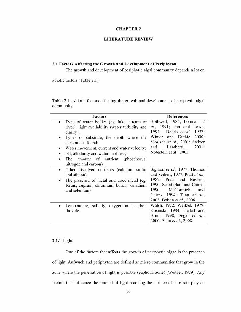
The growth and development of periphytic algal community depends a lot on
abiotic factors (Table 2.1):
Table 2.1. Abiotic factors affecting the growth and development of periphytic algal community.
Factors References
• Type of water bodies (eg. lake, stream or river); light availability (water turbidity and clarity);
Bothwell, 1985; Lohman et
al., 1991; Pan and Lowe, 1994; Dodds et al., 1997; Winter and Duthie 2000; Mosisch et al., 2001; Stelzer and Lamberti, 2001; Notestein at al., 2003.
• Types of substrate, the depth where the substrate is found;
• Water movement, current and water velocity; • pH, alkalinity and water hardness; • The amount of nutrient (phosphorus,
nitrogen and carbon) • Other dissolved nutrients (calcium, sulfur
and silicon); Sigmon et al., 1977; Thomas and Seibert, 1977; Pratt et al., 1987; Pratt and Bowers, 1990; Scanferlato and Cairns, 1990; McCormick and Cairns, 1994; Tang et al., 2003; Boivin et al., 2006.
• The presence of metal and trace metal (eg. ferum, cuprum, chromium, boron, vanadium and selenium)
• Temperature, salinity, oxygen and carbon dioxide
Walsh, 1972; Weitzel, 1979; Kosinski, 1984; Herbst and Blinn, 1998; Segal et al., 2006; Shun et al., 2008.
2.1.1 Light
One of the factors that affects the growth of periphytic algae is the presence
of light. Aufwuch and periphyton are defined as micro communities that grow in the
zone where the penetration of light is possible (euphotic zone) (Weitzel, 1979). Any
factors that influence the amount of light reaching the surface of substrate play an
11
important role on the growth of periphytic algae (Weitzel, 1979; Meulemans, 1987;
Paul and Duthie, 1989; Dodds, 1989; Kuhl and Jorgensen, 1994; Dodds et al., 1999;
Glud et al., 1999; Guasch et al., 2003).
A study by Evans and Stockner (1972) at Lake Winnipeg, Manitoba, found
that most of the periphytic biomass accumulation occurs at a depth between 10 cm to
25 cm. The study also found that blue-green algae dominated the area at a depth of 0
cm to 10 cm. Species such as Synedra ulna v. contracta (Ehrenberg), Gomphonema
constrictum v. capitata (Ehr.) Cleve, Rhoicosphena curvata (Kuetz.) Grunow and
�itzschia cf. fonticola (Grunow) were found at the depth between 5 cm to 25 cm,
while �avicula gracilis (Ehrenberg) [= �. tripunctata (O. F. Muell.) Bory v.
tripunctata] and �. cryptocephala (Kuetzing) were mostly found at a depth between
90 cm to 120 cm. Evans and Stockner (1972) concluded that the amount of light
penetrating the water was an important factor that influences the growth and
development of periphyton on natural or artificial substrates.
2.1.2 Substrate Suitability
Another factor that influences the growth of periphyton is the type and the
availability of substrates. Blum (1956) stated that true river algae depend largely on
rocky substrates and can mostly be found in fast flowing rivers. On sandy and
shifting riverbeds where the turbidity was high, Nelson and Scott (1962) found that
the presence of periphyton was low except on hard stable surfaces.
The abundance of periphyton in a river system depends largely on the type of
substrates at that particular place. The growth of periphyton on a granite surface is
12
higher compared to the growth on a limestone and sandy surface (Weitzel, 1979).
McConnell and Sigler (1959) found out that the surface of small pebbles support
higher chlorophyll content per unit area (m2) compared to larger rocks on the
riverbed.
Larger species of periphyton are normally found on stable objects compared
to epiphytic species. Other researchers also found significant differences in the type
of community on different types of substrate. The same species can be found on
different substrate but at a different level of abundance (Weitzel, 1979). According to
Round (1964), the condition and the characteristic of the sediment influence the
epipelic algal community. Potapova et al. (2005) mentioned that some cyanobacteria
such as Calothrix parietina, Homoeothrix janthina and the diatom Coconeis
neodiminuta are often associated with sandy sediments.
Epiphytic algae and diatom attached themselves on substrates using secretion
in the form of jelly, while other periphyton use stalks or gelatinous branches (Round,
1964). Therefore, the different strength of attachment in the form of jelly or
gelatinous method influences the presence of a particular species on a certain
substrate (Weitzel, 1979).
2.1.3 Water Movement
Movement of water such as velocity, wave, current and the circulation of
water in a lake influence the growth and biomass of periphyton. The movement of
water act as an inhibitor or as a catalyst for periphyton growth depending on its force
and direction (Weitzel, 1979). Water movement is important because flowing water
13
brings with it important nutrients that are needed for the growth and productivity of
periphyton while flushing away the byproducts of its metabolic activities (Duffer,
1966; Blum, 1956; Hynes, 1972; McConnell and Sigler, 1959; Odum, 1956;
Whitford, 1960; Weitzel, 1979). Biggs (1996) mentioned that a stable flow of water
usually promotes the accumulation of algal biomass in streams. This similar pattern
was also observed by Potapova et al., (2005) during their study in the Boston
metropolitan area. Streams that had more variable flow patterns or higher disturbance
level associated with stream flashiness (rate of change in flows) would lower algal
biomass and diversity and affect species composition (Biggs et al., 1998). Flow
variability in terms of discharges or stage variability, may affect algal assemblages at
different temporal scales (Clausen and Biggs, 1997; Matthaei et al., 2003; Potapova
et al., 2005).
The productivity of organism is influenced by water movement. Only diatoms
that are attached using jelly or gelatinous stalks can endure and survive in places
where the velocity of water is moderate or high (Patrick, 1948). High periphytic
assemblages in rivers and streams can mostly be found in sheltered area and in ponds
where the water is calm along the riverbanks. Apart from influencing the attachment
ability of periphytic organism, water movement can also influence the solubility and
the availability of dissolved substances such as oxygen, carbon dioxide and other
nutrients. Water movement also influences the temperature, turbidity and
transparency of water (Patrick, 1948; Weitzel, 1979).
Flowing water with high velocity becomes an inhibitor to the growth of
periphyton due to its shearing effect even though there are a few species of
14
filamentous algae that require an environment where the water velocity is high
(Blum, 1956; Whirford, 1960; Weitzel, 1979). It was observed that when flood
occurred and water velocity in streams increased, the periphyton on the various
substrates was peeled away by stream flow (Yamada and Nakamura, 2002).
The type of substrates also plays an important role in determining the
influence of water velocity on the growth of periphyton. Periphyton that grows on
sandy surfaces are more vulnerable to erosion compared to periphyton that grows on
the surface of a rock even if they are located at a place where the water moves slowly
(Duffer and Dorris, 1966; Nelson and Scott, 1962; Neel, 1968; Weitzel, 1979).
McConell and Sigler (1959) observed that productivity was high in places with slow
moving water. This finding is similar to an earlier research by Butcher (1932) which
showed that high biomass value was obtained at sites where the water flow was slow.
2.1.4 Dissolved Substances
The role played by dissolved substances is also important. Patrick (1948)
discovered that most diatoms had a high abundance when calcium carbonate
concentration was 3.0 mg/liter and above, while the concentration of silicate was at
0.5 mg/L and above. This is because apart from being a buffer for pH, calcium also
reacts with toxic ion and control the concentration of sulfuric acid (Weitzel, 1979).
Metals and trace elements cause different reactions when exposed to different types
of algae species. There are some diatoms that can tolerate copper concentration
between 1.5 mg/L to 2.1 mg/L even though at this level it is toxic to many algal
species (Patrick, 1948; Weitzel, 1979). A study by Patrick et. al. (1975) also found
that the presence of several trace elements changed the community structure from
15
one that was dominated by diatoms to a community that was dominated by blue-
green algae. They also found that diatom was dominant with higher species diversity
when chromium concentration was between 40 µg/liter to 50 µg/liter. In contrast, a
concentration of chromium between 95 µg/liter to 97 µg/liter lowered the diatoms
diversity even though the abundance was still high. Boron also played an important
part in determining the community structure of algal assemblages. A concentration of
1.0 µg/liter of boron caused a change from a community of diatom to a community
of blue-green algae, while the presence of nickel at any concentration was toxic to
diatoms but it was preferable for the growth of blue-green algae, such as
Stigeoclonium lubricum (Dillw.) Kuetzing (Patrick et. al., 1975; Weitzel, 1979).
Potapova et al., (2005) also mentioned that the concentration of dissolved solids
would influence the assemblage’s patterns.
Metals and trace elements are toxic to a lot of algae species. Generally
diatoms are more vulnerable to the presence of trace elements compared to blue-
green algae such as Stigeoclonium lubricum (Dillw.) Kuetzing. The effect of metals
and trace elements on diatom can be seen from the reduced concentration of
chlorophyll a (Weitzel, 1979). Apart from that, cell deformities have also been
associated with contamination by heavy metals (McFarland et al., 1997). Studies
have also found that extreme metal contamination from mining activities could
decrease the number diatom taxa (Juttner et al., 1996; Medley and Clements, 1998;
Stewart et al., 1999; Genter and Lehman, 2000; Verb and Vis, 2000; Fore and Grafe,
2002).
16
2.1.5 �utrients
The increase of nutrients in streams and water body have been linked to the
changes of autotrophic community composition, vegetative biomass and an increase
of nuisance species (Wright and McDonnell, 1986a, 1986b; Notestein et al., 2003).
This in turn, affects the community structure and alters the food web dynamic of a
given system (Hershey et al., 1988; Peterson et al., 1993).
It was found that an increase in nutrient concentration would influence
periphyton abundance (Notestein et al., 2003). An increase in nitrogen alone would
stimulate periphyton growth (Stelzer and Lamberti, 2001) especially when light was
not a limiting factor (Lohman et al., 1991; Mosisch et al., 2001). The addition of
phosphorus whether solely or concurrently with nitrogen was also found to increase
periphyton abundance (Bothwell, 1985; Pan and Lowe, 1994; Dodds et al., 1997;
Winter and Duthie, 2000). Similar results were also obtained by Notestein et al.,
(2003) which suggested that phosphorus might be the primary nutrient limiting factor
for periphyton growth in coastal stream in Florida.
McCormick et al., (2001) observed that two distinct periphyton assemblages
developed in response to increase phosphorus loading. These assemblages were
characterized by higher phosphorus content, lower N:P ratios and higher biomass-
specific productivity compared to oligotrophic assemblages (McCormick et al.,
2001). Intermediate phosphorus loads was found to change the dominance from
cyanobacteria to filamentous chlorophytes, such as Spirogyra, while a high loading
rates resulted in a direct shift from oligotrophic to eutrophic cyanobacteria (e.g.
Plectonema wollei, Oscillatoria princeps) (McCormick et al., 2001). Similar results
17
were also obtained by other studies where many were enriched simultaneously by
both nitrogen and phosphorus (Howard-Williams, 1981; Hillebrand, 1983;
McDougal et al., 1997; Havens et al., 1999).
2.1.6 Periphyton Predation and Competition
Apart from the abiotic environment, biotic interaction such as grazing and
competition also plays an important part in the colonisation of periphyton on hard
substrates in freshwater (Feminella and Hawkins, 1995; McCormick, 1996) and
marine habitats (Hillebrand and Sommer, 1997; Hillebrand et al., 2000). Hillebrand
and Kahlert (2002) observed that the presence of grazer can reduce periphyton
biomass by 50% in Lake Erken. Other studies revealed that up to 90% of available
algal biomass was consumed by grazers and this is especially true for periphyton
found on hard substrate (Feminella and Hawkins, 1995; Hillebrand et al., 2000).
Grazers such as snails (McClatchie et al., 1982), crustaceans (Hargrave, 1970;
Gerdol and Hughes, 1994) and annelids (Smith et al., 1996) was found to have a big
influence on biomass and community structure of periphyton.
Hillebrand and Kahlert (2002) also observed that the effects of macrograzer
were lesser on periphyton that grows on sediment as compared to those that grows on
hard substrate. In an earlier study, Hillebrand and Kahlert (2001) noted that strong
grazing pressure of epilithic benthic algae were evidence in Väddö and Lake Erken.
Earlier study done by Cattaneo and Kalff (1986) found that smaller fauna
such as oligochaete and cladocerans also had similar effects on algal biomass as
macrograzers. Due to this, Sunbäck et al. (1996) and Epstein (1997a, b) proposed
18
that micro and meiofauna are able to consume most of the primary production in
sediments (Hillebrand and Kahlert, 2002). However, it is not clear whether small
fauna can influence the algal biomass in a longer time scale (several weeks).
A close relationship between some invertebrate and periphyton were
observed in Lake Iznik. An increase of nematodes resulted in the decrease of stalked
and tube diatoms (Albay and Aykulu, 2002). They also found that Rotifers (mainly
Lophocharis sp.) and Ciliates also have a negative impact on erect and cocconeis
type diatoms. Rotifer also has a negative relation with prostrate diatoms. However
Rotifer was found to have a positive relationship with Cyanophytes. Nematodes
(mainly Anonchus sp. and Microlaimus sp.) on the other hand, have a negative
relationship with Cyanophytes (Albay and Aykulu, 2002).
A study on the effects of snail grazing on periphyton found that grazing have
a significant effect on the composition of periphyton communities (Marks and Lowe,
1989). It was observed that the relative biovolume of green algae increase to 93%
from 64% on graze substrate (Marks and Lowe, 1989). Periphyton communities that
were highly grazed would usually be dominated by prostrate species that adhere
tightly to the substrate or by small understory species that were not grazed due to
their small size (Hunter, 1980; Hunter and Russel-Hunter, 1983; Sumner and
McIntire, 1982; Marks and Lowe, 1989). Grazing has been known to physiologically
maintain periphyton communities in an earlier succession stage (Marks and Lowe,
1989), meaning that the development of the periphyton community into a mature
state had been retarded due to grazing.
19
Competition for nutrient and habitat also effects periphyton growth.
Brammner (1979) and Brammer and Wetzel (1984) observed that Stratiotes
competes with phytoplankton for nutrients from the surrounding water. This
competition had resulted in the decreased of phytoplankton density in the water
where Stratiotes is dominant (Brammer, 1979; Brammer and Wetzel, 1984).
Submerged macrophytes have been found to compete with other autotrophic
organisms such as algae and periphyton and limit their growth (Kufel and Ozimek,
1994; Von Donk and Van de Bund, 2002; Mulderij et al., 2005b). The macrophytes
was also found to excrete allelophathic substances that inhibit phytoplankton growth
(Gross, 2003; Mulderij et al., 2005b). It was reported that allelopathic activities of
macrophyte such as Chara (Wium-Andersen et al., 1982; Blindow and Hootsmans,
1991; Mulderij et al., 2005a), Ceratophyllum (Jasser, 1995; Mjelde and Faafeng,
1997) and Myriophyllum (Jasser, 1995; Gross et al., 1996) could resulted in changes
in phytoplankton composition and biomass (Mulderij et al., 2005b).
2.2 Periphytic Algal Attributes as Indicators of Aquatic Degradation
Even though physical and chemical variables are widely used in monitoring
water quality due to its ability to detect changes in the environment in a quick and
straightforward manner, it also has its disadvantages of not being able to reflect the
changes in water quality on biological communities (Vis et al., 1998). The mixture of
organic and inorganic compounds in most urban effluent further complicates the
monitoring process due to the high cost required for the analyses (Vis et al., 1998).
Therefore, the use of periphyton has several advantages compared to the traditional
method of using physical and chemical variables to determine water quality. Among
20
the advantages of using periphyton as an indicator are; they are easy to collect,
taxonomically diverse and have a short regeneration time which means that it can
react quickly to changes in stream water quality (Hill et al., 2000; Wan Maznah and
Mansor, 2000). Fore and Grafe (2002) also concluded that diatoms might represent a
biological alternative to fish when assessing water quality in rivers or sites that were
too deep to effectively sample fish or when endangered or protected species
prohibited sampling. Apart from that, where cases of chemical and biological
(faunal) information disagree about a site condition, diatoms can provide clues to
resolve the conflict due to their sensitive nature to water chemistry (Fore and Grafe,
2002).
Various researches have showed that major changes in water quality can
influence the characteristic of periphyton. Characteristics of periphyton such as
biomass (Wuhrmann and Eichenberger, 1975; Watanabe et al., 1988; Biggs, 1989),
diversity indices (Weitzel and Bates, 1981; Stevenson, 1984; Stewart and Robertson,
1992; Vis, 1998; Hillebrand and Sommer, 2000), biotic indices (Descy and Coste,
1991; Kelly et al., 1995) and taxonomic composition (Archibald, 1972; Rott, 1991)
can be used as an indicator of water quality. Some studies have also found that algal
community structure (Cattaneo et al., 1995; Wan Maznah and Mansor, 2002) and
periphyton productivity (Ho, 1976; Anton et al., 1998) can also be used to determine
water quality (Wan Maznah and Mansor, 2000; Wan Maznah, 2002).
The use of periphyton as a water quality indicator has been widely accepted.
Researchers have developed several schemes that classified organisms according to
the amount of organic pollutants associated with their occurrence. A system that
21
classified water system as eutrophic, mesotrophic or oligotrophic was developed by
using the correlation between the type of species that existed at different levels of
pollution (Weitzel, 1979). The terms eutrophic, mesotrophic and oligotrophic refers
to the level of nutrients that are high, moderate and low (Round, 1964).
Eutrophication is defined as the process in which water bodies are made more
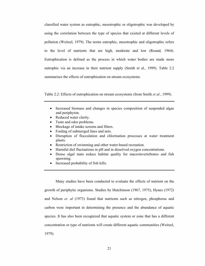
eutrophic via an increase in their nutrient supply (Smith et al., 1999). Table 2.2
summarises the effects of eutrophication on stream ecosystems.
Table 2.2: Effects of eutrophication on stream ecosystems (from Smith et al., 1999).
• Increased biomass and changes in species composition of suspended algae and periphyton.
• Reduced water clarity. • Taste and odor problems. • Blockage of intake screens and filters. • Fouling of submerged lines and nets. • Disruption of flocculation and chlorination processes at water treatment
plants. • Restriction of swimming and other water-based recreation. • Harmful diel fluctuations in pH and in dissolved oxygen concentrations. • Dense algal mats reduce habitat quality for macroinvertebrates and fish
spawning. • Increased probability of fish kills.
Many studies have been conducted to evaluate the effects of nutrient on the
growth of periphytic organisms. Studies by Hutchinson (1967, 1975), Hynes (1972)
and Nelson et. al (1973) found that nutrients such as nitrogen, phosphorus and
carbon were important in determining the presence and the abundance of aquatic
species. It has also been recognized that aquatic system or zone that has a different
concentration or type of nutrients will create different aquatic communities (Weitzel,
1979).
22
The concept of using organisms as an indicator has been widely used to
determine the level of pollution. Patrick and Hohn (1956) and Patrick and Reimer
(1966) had discussed on developing and using indicator community to monitor
pollution. Aquatic ecosystems was defined as “healthy”, “semi-healthy”, “polluted”
and “severely polluted” based on the quantitative evaluation of the number of diatom
species (Patrick, 1949; Patrick and Hohn, 1956; Patrick and Reimer, 1966). The
scheme is based on the concept of ‘indicator organisms’ that live in different types of
environment where it can be used to represent a general level of pollution, and the
relative abundance of particular indicator species that are used must be significant.
Diatoms are good ecological indicators because they are found in abundance
in most lotic ecosystem (Stevenson and Bahls, 1999). Since diatoms can be found in
a wide range of ecological conditions, it can provide multiple indicators of
environmental change.
There are also disadvantages of using periphyton as a bioindicator. Even
though the changes in nutrient concentration in water had been linked to changes in
periphyton community, its influence had been variable or inconsistent (Vis, 1998;
Notestein et al., 2003). For example, experiments on the effect of nutrient
enrichment on algal density in freshwater has been contradictory. Marcus (1980) and
Pringle (1990) reported an increase in algal density due to the increase in nutrient
supply, but Miller et al. (1992) reported the opposite. Furthermore, some studies
reported that nitrogen alone would stimulate periphyton growth (Stelzer and
Lamberti, 2001) when light was not a limiting factor (Lohman et al., 1991; Mosisch
et al., 2001). Moreover, studies by Bothwell (1985), Pan and Lowe (1994) showed
23
that the addition of phosphorus and nitrogen increased periphyton abundance. Dodds
et al., (1997) and Winter and Duthie (2000) on the other hand, observed an increase
in periphyton abundance when it was concurrently enriched with phosphorus and
nitrogen.
Even though some researches found that the addition of phosphorus, and
nitrogen plus phosphorus resulted in greater biomass, they also noticed that the
addition of nitrate alone showed not much difference in periphyton biomass from the
controls (Notestein et al., 2003). Further analysis, showed that the differences
between the treatments containing phosphorus alone, phosphorus plus nitrogen, and
nitrogen alone were not significant (Notestein et al., 2003). Thus, making the
differentiation of the effects of phosphorus, phosphorus plus nitrogen and nitrogen
difficult.
Sand-Jensen (1983) highlighted several reasons why it was not possible to
accurately determine when and how physico-chemical parameters affected the
growth of periphytic algae. The first reason was when periphyton growth patterns
were examined in a fluctuating natural habitat, it was difficult to pinpoint a single
regulating factor since there were many physico-chemical parameters that influenced
periphyton growth. Sand-Jensen (1983) argued that the autotrophic and heterotrophic
processes that happened internally within the boundary layer would change the
chemical condition and could be different from the free water phase. The change in
the chemical condition within the periphytic community depended on the rate of
exchange with the free water process or the balance of opposing process within the
periphytic layer. Another reason was that most measurements of physico-chemical
24
only focused on the free-water phase above the periphytic community and not within
the community where the condition was different. The growth rates of periphytic
algae also were either difficult or impossible to measure directly (Sand-Jensen,
1983).
Apart from the variable response to nutrient enrichment, the viability of
periphyton as an indicator is also under threat from the grazing activity of
invertebrate and fishes. It was reported that the grazer would increase the grazing
pressure to periphyton due to enhanced food availability and this situation could
offset the effect of nutrient enrichment (Hillebrand et al., 2000, 2002; Hillebrand and
Kahlert, 2001; Hillebrand, 2002; Cosgrove et al., 2004).
The inconsistencies in the periphyton reaction to the changes in water quality
are likely caused by natural variability associated with periphytic communities
(Weitzel et al, 1979; Morin and Cattaneo, 1992; Vis, 1998) and the differences
between systems under study (i.e. stream vs river, temperate vs tropical region). The
complex interaction of physical, chemical and biological factors that influence
periphytic communities makes it difficult to detect water quality related changes in
periphyton (Vis, 1998). This can be seen in a study by Guasch et al., (2003) where
apart from the river water quality and light, the physical structure and biotic activity
in the dense biofilm also plays a significant role in determining the condition within
the matrix. Their study shows that the responses of periphyton toward the
concentration of organic and inorganic substances in the water are influenced by
their physiological state and density (Guasch et al., 2003). The thickness of
periphyton can causes the creation of marked gradients of light (Meulemans, 1987;