Embed Size (px)
Citation preview
WATER QUALITY ENHANCEMENT ASSESSMENT
OF AN EXISTING FLOOD CONTROL DETENTION
FACILITY IN THE CITY OF TULSA, OKLAHOMA
By
STEVEN PHILLIP SCHAAL
Bachelor of Science in Agriculture
Southwest Texas State University
San Marcos, Texas
1994
Submitted to the Faculty of the Graduate College of the
Oklahoma State University in partial fulfillment of
the requirements for the Degree of
MASTER OF SCIENCE July, 2006

ii
WATER QUALITY ENHANCEMENT ASSESSMENT
OF AN EXISTING FLOOD CONTROL DETENTION
FACILITY IN THE CITY OF TULSA, OKLAHOMA
Thesis Approved:
Wm. Clarkson
Thesis Advisor
Joseph R. Bidwell
John N. Veenstra
A. Gordon Emslie
Dean of the Graduate College

iii
TABLE OF CONTENTS
Chapter Page
I. INTRODUCTION......................................................................................................1
Project Background..................................................................................................2Objectives and Scope...............................................................................................4Site Description........................................................................................................4
II. REVIEW OF LITERATURE
Factors Affecting Stormwater Treatment Wetland Design .....................................7Inflow Characteristics ..............................................................................................7Detention Time ........................................................................................................9Wetland Characteristics .........................................................................................11Sampling Methods .................................................................................................14Properties of Rhodamine WT & General Fluorometric Procedures for Dye Tracing.................................................................................................15
III. METHODOLOGY
Water Quality Analysis..........................................................................................17Sampling Procedures for Water Quality ................................................................17Sampling Procedures for Dye Testing ...................................................................18Sampling Procedures for Subsequent Events ........................................................20
iv
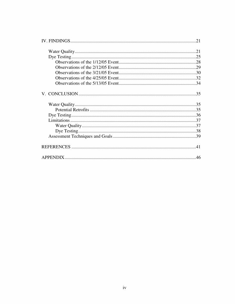
IV. FINDINGS.............................................................................................................21
Water Quality.........................................................................................................21Dye Testing............................................................................................................25
Observations of the 1/12/05 Event...................................................................28Observations of the 2/12/05 Event...................................................................29Observations of the 3/21/05 Event...................................................................30Observations of the 4/25/05 Event...................................................................32Observations of the 5/13/05 Event...................................................................34
V. CONCLUSION......................................................................................................35
Water Quality.........................................................................................................35Potential Retrofits ............................................................................................35
Dye Testing............................................................................................................36Limitations .............................................................................................................37
Water Quality...................................................................................................37Dye Testing......................................................................................................38
Assessment Techniques and Goals ........................................................................39
REFERENCES ............................................................................................................41
APPENDIX..................................................................................................................46
v
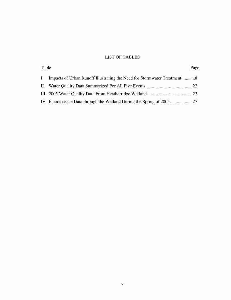
LIST OF TABLES
Table Page
I. Impacts of Urban Runoff Illustrating the Need for Stormwater Treatment............8
II. Water Quality Data Summarized For All Five Events .........................................22
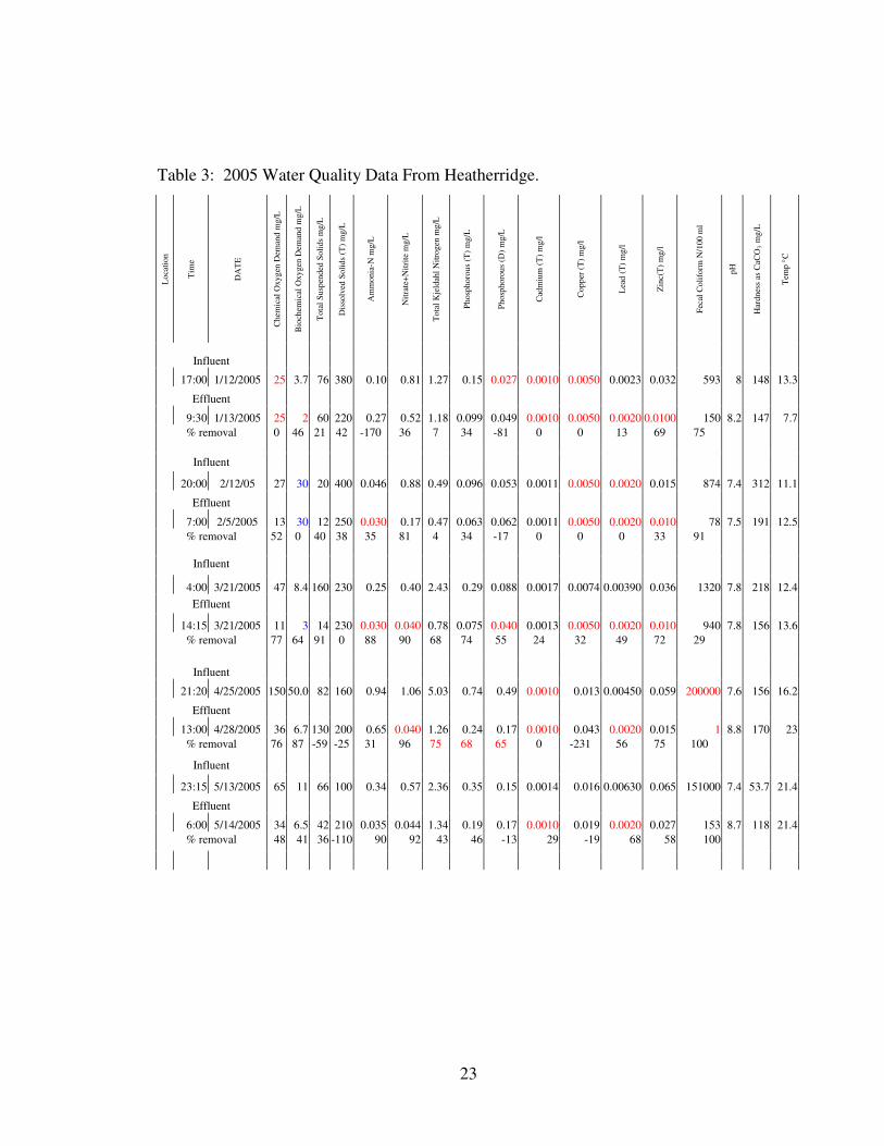
III. 2005 Water Quality Data From Heatherridge Wetland ........................................23
IV. Fluorescence Data through the Wetland During the Spring of 2005....................27
vi
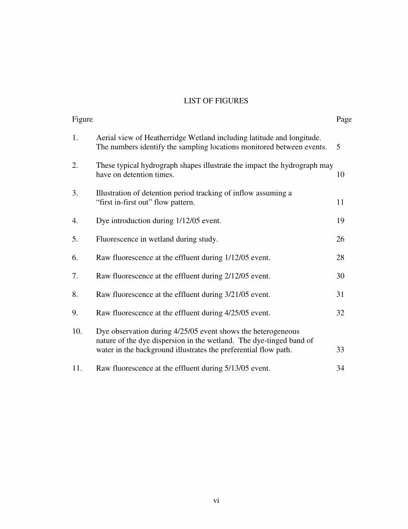
LIST OF FIGURES
Figure Page
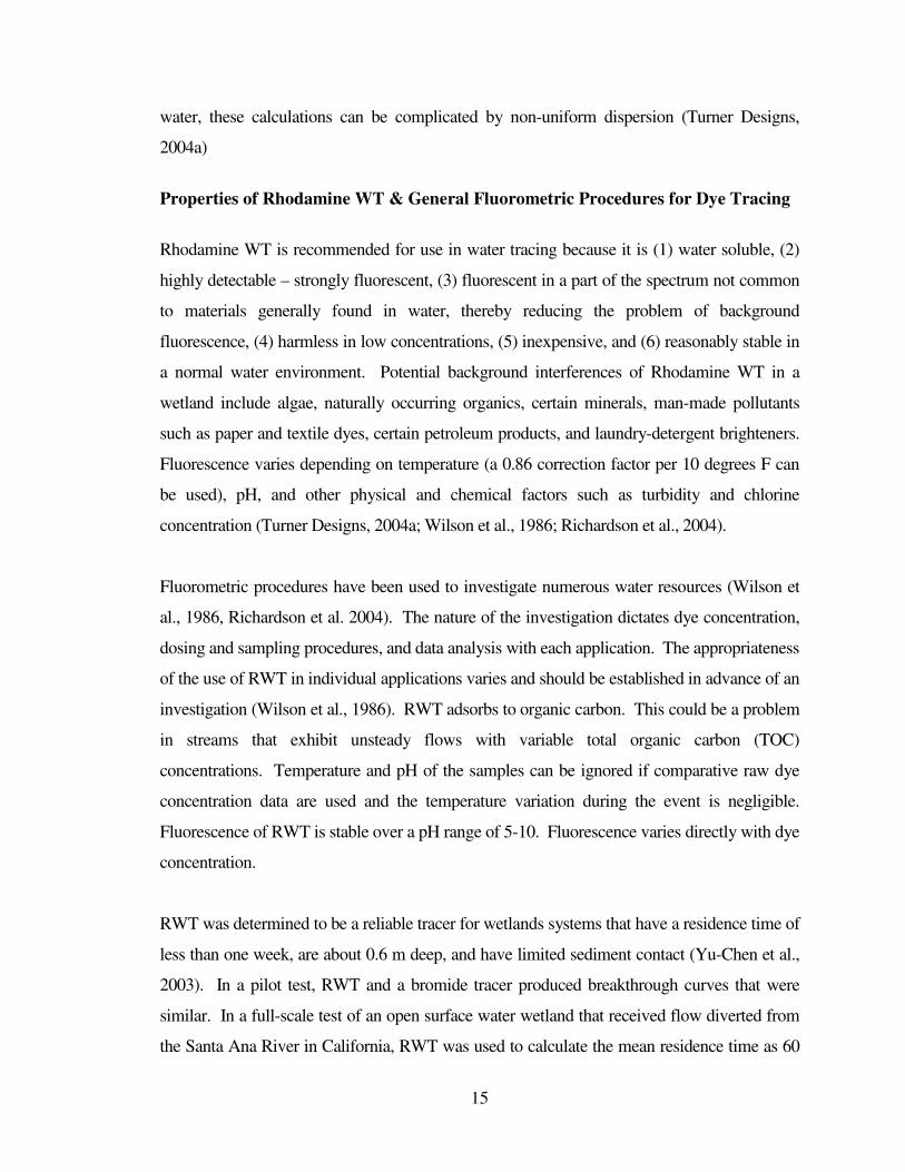
1. Aerial view of Heatherridge Wetland including latitude and longitude.The numbers identify the sampling locations monitored between events. 5
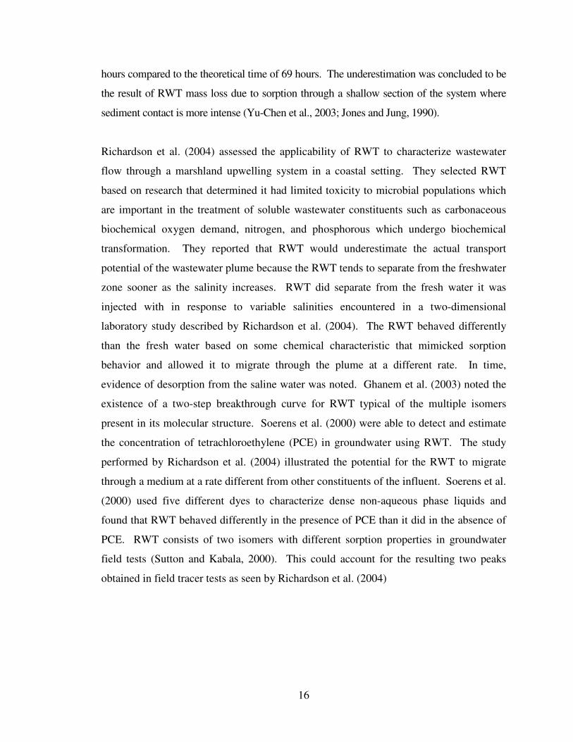
2. These typical hydrograph shapes illustrate the impact the hydrograph mayhave on detention times. 10
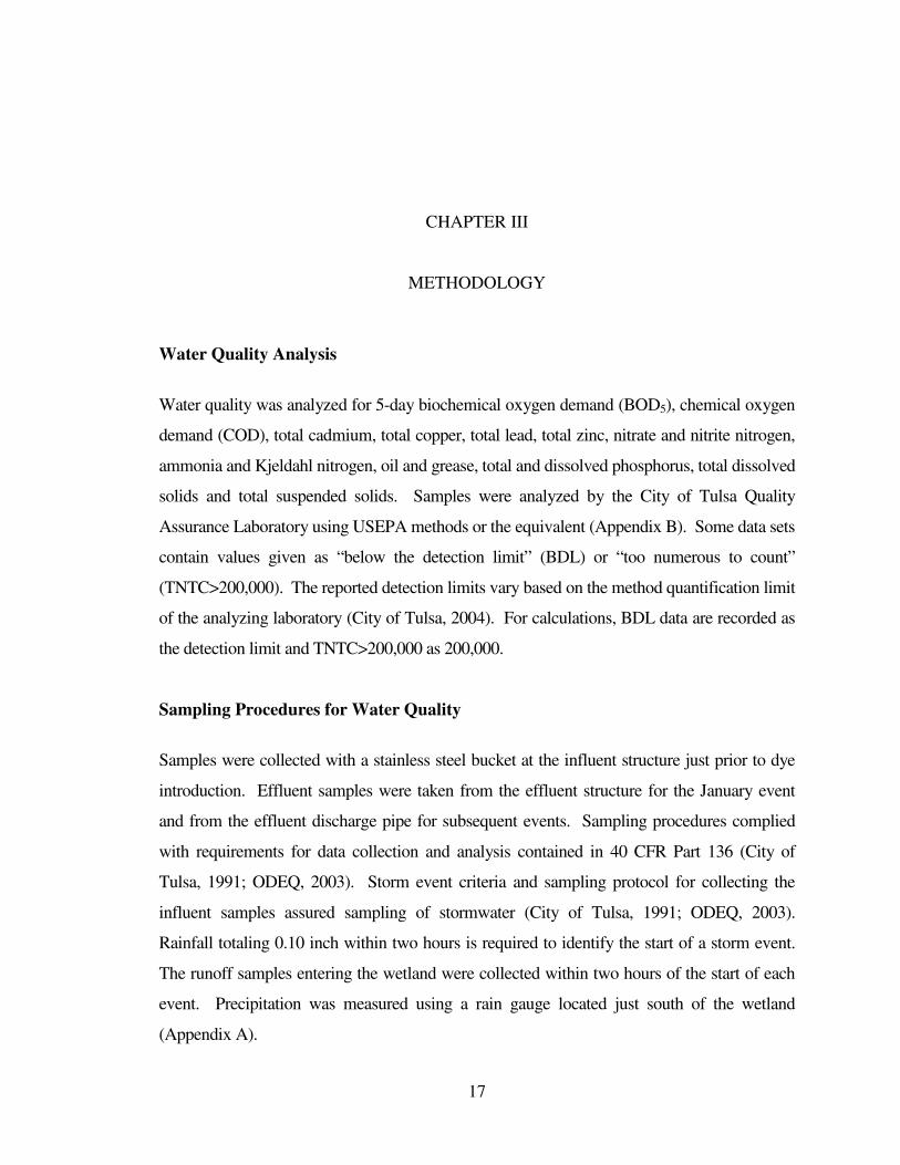
3. Illustration of detention period tracking of inflow assuming a“first in-first out” flow pattern. 11
4. Dye introduction during 1/12/05 event. 19
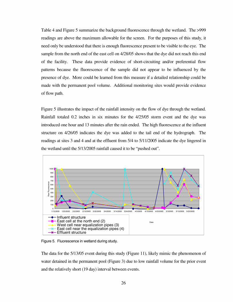
5. Fluorescence in wetland during study. 26
6. Raw fluorescence at the effluent during 1/12/05 event. 28
7. Raw fluorescence at the effluent during 2/12/05 event. 30
8. Raw fluorescence at the effluent during 3/21/05 event. 31
9. Raw fluorescence at the effluent during 4/25/05 event. 32
10. Dye observation during 4/25/05 event shows the heterogeneousnature of the dye dispersion in the wetland. The dye-tinged band ofwater in the background illustrates the preferential flow path. 33
11. Raw fluorescence at the effluent during 5/13/05 event. 34
1
CHAPTER I
INTRODUCTION
From ancient civilizations to the present, waste streams have been directed to wetlands for
treatment and disposal. During the early part of this century many wetlands were drained and
altered, and their functions lost. Now wetlands are recognized as among the most productive
and valuable ecosystems providing an abundance of flora and fauna, wildlife habitat and flood
control. Constructed wetlands have been built to duplicate many of these benefits and
functions, often times designed for a multitude of reasons to accommodate the need for human
development (Kentula 2002; Lipa and Strecker, 2004; Strecker, et al. 2001; Carter Burgess,
Inc., 2001). Stormwater has been identified as a source of pollution to urban streams, carrying
any number of pollutants associated with various uses of the land. Since the promulgation of
the Clean Water Act and the National Pollution Discharge Elimination System program,
constructed wetlands have been added to the list of Best Management Practices (BMP) that
Municipal Separate Storm Sewer System (MS4) utility managers can incorporate into
stormwater management plans to address the impacts of human development on urban
streams (City of Tulsa, 1994). This study’s attempt to assess the effectiveness of this BMP
testifies to today’s awareness of the impact of stormwater runoff and the value of the
beneficial uses ascribed to urban water bodies.
The City of Tulsa, as an owner and operator of an MS4, is required to evaluate the
effectiveness of the management practices used to ensure that the stormwater discharged into
waters of the state is of good quality and relatively contaminant-free. One such BMP is the
Heatherridge Stormwater Detention Facility (Heatherridge). Heatherridge was constructed as
a dual-purpose flood control facility and constructed wetland to mitigate the impact on
wetlands due to the construction of the Creek Nation Turnpike through the southeast region of
Tulsa, Oklahoma (BKL, 1991). Since its construction, the City of Tulsa has gathered data on
2
samples taken from the influent and effluent structures of the wetland during several storm
events, assuming a twelve-hour detention time based on an engineering estimate (City of
Tulsa, 1999). The City has concluded from the data that water quality is enhanced by the
wetland (Haye, 1999). This study will gather water quality data (as defined by the
concentration of various elements and compounds) from both the influent and the effluent of
this constructed wetland facility utilizing Rhodamine WT (RWT) dye as a tool to help identify
the detention time.
Project Background
The City of Tulsa, with a population of 375,000, covers 200 square miles of gently rolling
terrain in northeastern Oklahoma. Tulsa, located on the Arkansas River, contains some 56
creeks and drainage basins. Rainfall averages 42.42 inches per year (National Weather
Service, 2005), with occasional heavy thunderstorms. Located in southeast Tulsa,
Heatherridge is a constructed wetland, created as part of a plan to mitigate approximately 15
acres of wetland, wetland habitat, riparian forest, and associated wildlife habitat impacted by
the construction of the Creek Turnpike in 1995 (Haye, 1995). Tulsa chose to build
Heatherridge in response to Section 404 of the Clean Water Act mandate to compensate for
impacted natural wetlands (EPA 1993). The drainage area is 240 acres, mostly residential and
light commercial land use. The detention basin was designed for a 100-year frequency storm.
As designed, the peak inflow is 1276 cubic feet per second (cfs), and the outfall is 38 cfs
maintained by a water level control structure. The volume of flood storage is 115 acre-feet
with a 12 hour design detention time. A permanent pool covers approximately nine acres of
the facility. Four zones of wetland plants were installed. Consultation for plant selection was
provided by the US Army Corps of Engineers, Lewisville Aquatic Ecosystem Research
Facility, Lewisville, Texas (US Army COE, 1995). The survival rate of these plants was
evaluated in 1999 and at the time, the rate was estimated to be “good” (Haye, 1999). The five-
year Monitoring Plan for the site did not include a water quality component (HNTB, 1990).
The 1972 amendments to the Federal Water Pollution Control Act (Clean Water Act) prohibit
the discharge of any pollutant to navigable waters from a point source unless the discharge is

3
authorized by a National Pollutant Discharge Elimination System (NPDES) Permit. The
Water Quality Act of 1987 broadens the requirements of the Clean Water Act to mandate a
phased approach to regulate stormwater discharges, through coverage under the NPDES
permit program. The first phase of regulation applied to the following stormwater discharges:
• Stormwater discharges associated with industrial activity;• Stormwater discharges from a municipal separate storm sewer system (MS4)
serving a population of 250,000 or more (a large system);• Stormwater discharges from a MS4 serving a population of more than 100,000
but less than 250,000 (a medium system);• Stormwater discharges regulated under an existing permit; and • Stormwater discharges designated by EPA or the State as contributing to the
violation of the water quality standard or as a significant contributor of pollutants to the waters of the United States.
The City of Tulsa, as an operator of a large MS4, filed a Notice of Intent to the USEPA
seeking coverage under the NPDES Storm Water Discharge Permit in 1990. Under the issued
permit, the City of Tulsa is required to meet certain terms and conditions, which include:
• Monitoring of representative stormwater discharges;• Development and implementation of Pollution Prevention and Public Awareness
Programs;• Development and implementation of maintenance schedules and protocols for the
stormwater management system;• Assessment of existing flood control facilities for potential structural
improvements to enhance water quality; and• Completion and submittal of Annual Reports describing the
progress/implementation of the programs listed above.
This study details an evaluation of Heatherridge, in the City of Tulsa, performed in accordance
with the requirements of the City of Tulsa’s current National Pollution Discharge Elimination
System permit, Proposed Management Program (EPA 2002). The Flood Control Project
section of the Storm Water Quality Management Programs for NPDES Permit #OKS000201
(Oklahoma Department of Environmental Quality, 2003) states:
”Impacts on receiving water quality shall be assessed for all flood management projects. The feasibility of retrofitting existing structural flood control devices to provide additional pollutant removal from storm water shall be evaluated.”
4
Retrofits are structural stormwater management measures for urban watersheds designed to
help minimize accelerated channel erosion, reduce pollutant loads, promote conditions for
improved aquatic habitat, and correct past mistakes. In order to determine if an existing
structural control device can benefit from retrofitting, one must first determine which benefits
to evaluate and the extent to which the facility is or is not affecting stormwater in its current
condition.
Objectives and Scope
The primary objective of this study is to quantify the degree of natural attenuation of specific
contaminants in stormwater as it passes through a constructed wetland. Retrofits to enhance
water quality of runoff from the Heatherridge watershed will be discussed. The secondary
objective will be to assess the effectiveness of the dye tracer as a tool to ensure the same parcel
of water was sampled at both the influent and effluent and in quantifying the detention time of
individual events.
Site Description
Heatherridge is an in-stream emergent vegetative constructed wetland in Tulsa, Oklahoma
(Figure 1). The landscape design incorporated plants selected to improve water quality (Smart
and Doyle, 1995; U.S. Army Corps Of Engineers, 1995). Heatherridge receives flow from
Fry Ditch 2 which flows southerly from a mixed residential, commercial watershed and enters
the west cell of Heatherridge via the influent structure which consists of a triple 8’X 8’
reinforced concrete box culvert, with gabion structures flanking both the upstream and
downstream sides. The west cell is connected to the east cell by an equalization structure
consisting of two 24” reinforced concrete pipes that run under a utility road as required by the
Oklahoma Turnpike Authority (OTA) as part of the wetland mitigation requirements
established by the US Army Corps of Engineers (BKL, 1992). A road separates the west and
east cells along a sanitary sewer line that remains in place due to the cost constraints related to
moving the line (Figure 1). There is a sedimentation basin just downstream of the influent
5
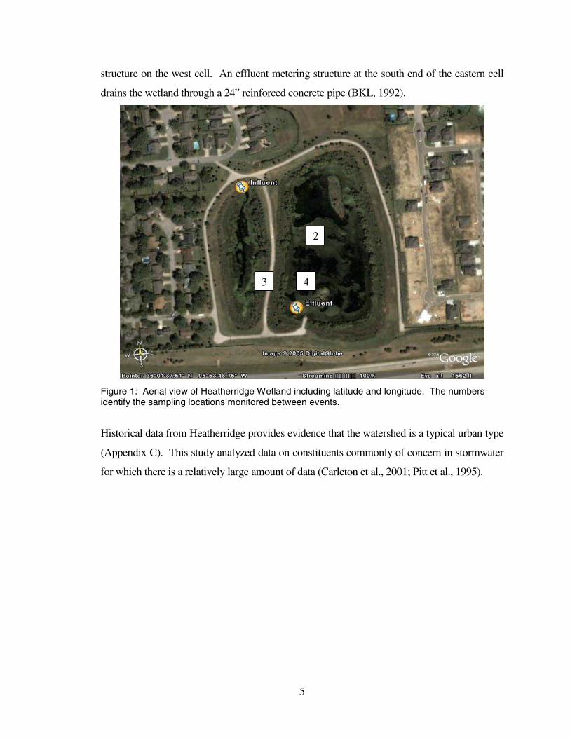
structure on the west cell. An effluent metering structure at the south end of the eastern cell
drains the wetland through a 24” reinforced concrete pipe (BKL, 1992).
Figure 1: Aerial view of Heatherridge Wetland including latitude and longitude. The numbers identify the sampling locations monitored between events.
Historical data from Heatherridge provides evidence that the watershed is a typical urban type
(Appendix C). This study analyzed data on constituents commonly of concern in stormwater
for which there is a relatively large amount of data (Carleton et al., 2001; Pitt et al., 1995).
2
3 4
6
CHAPTER II
REVIEW OF LITERATURE
The science of wetland creation is a growing field of scientific endeavor (Whigham, 1999).
Current regulatory policy has a goal of “No Net Loss” of wetlands, and the Corps of
Engineers requires an assessment of the functions of a wetland as part of their permitting
process. In some cases the debate of the success or failure of this policy revolves around
whether a created wetland can replace a natural wetland in terms of value or function. Some
restored or created wetlands mimic functions of natural wetlands, but the similarity depends
upon the assessment procedure. Many wetland assessment methods emphasize the
importance of the role the wetland plays in the ecosystem (Brinson, 1993; Whigham, 1999;
Bidwell and Gorrie 1998). The success or failure of a constructed wetland project is relative
to the goal of each project and what measurement criteria are used in the assessment. The
design criteria for a created wetland may include the project goal of recreating a particular
function. This being said, it is theorized that a constructed wetland in a residential watershed
can decrease contaminant loading to the ultimate receiving body of water (Oklahoma
Conservation Commission, 1996) and is often addressed during the design phase as a goal of
the project. Pollution removal in a constructed wetland is highly dependent on runoff and
wetland hydrology. Storms occur at irregular intervals, which affects the amount of runoff.
They vary widely in intensity and duration, which affects pollution loading by affecting runoff
volume. They occur in all seasons and impact wetlands at differing vegetative states.
Wetlands vary widely in volume, surface area, and vegetation cover. The functions performed
by wetlands are dependant on the above characteristics (Meshek and Associates, 1998). An
understanding of these characteristics will help with the evaluation. This literature survey
examines some of the many factors that must be addressed.
7
Factors Affecting Stormwater Wetland Design
Stormwater utility managers consider stormwater contaminants in urban watersheds as they
choose appropriate management practices to match the goal of the management plan. When a
specific contaminant is the focus of the management plan, the design of the wetland must
optimize those functions which best attenuate that pollutant. Flood attenuation is often a
primary concern. Wildlife habitat, passive and active recreation and a multitude of other
factors can be considered. Research has helped to define the nature of stormwater runoff from
residential land uses by identifying how many human influences, within the watershed, affect
pollutant loading and the hydrologic regime. Table 1 (Monroe County, 2005) identifies
typical pollutants and their impacts. These human impacts are site specific depending on
population. The parameters chosen for this study and the historical data of the study site are
similar to the conventional stormwater pollutants (Pitt et al., 2004; Carleton et al., 2001;
Heatherridge Historical and Removal Efficiency Data, Appendix C). It is important to
consider the impact stormwater pollutants have on the environment. This will help decide
appropriate controls based on the overall objective of the management plan. For example, the
interrelations of pollutants may make it advantageous to target suspended solids to capture a
portion of the total phosphorous Carleton et al., 2001).
Inflow Characteristics
Water quality parameters frequently lump individual chemical compounds into a class of
materials (Kadlec, 2002). For example: total suspended solids (TSS) can include an organic
fraction and an inorganic fraction. Biological oxygen demand (BOD) can result from grass
clippings or animal waste. Within these lumped parameters there are compounds with varying
biological and chemical decomposition rates. The overall concentration of BOD and other
lumped parameters tells only some of the story of the nature and quality of the stormwater
runoff (Kadlec, 2002).

8
Table 1: Impacts of Urban Runoff Illustrating the Need for Stormwater Treatment
CategoryCategory ParametersParameters Possible Sourcesossies EffectsEffects
Sediments Organic & Inorganic: Total Suspended Solids Turbidity Dissolved Solids
Construction Sites Urban/Agriculture Landfills Septic Tanks
Turbidity Habitat Alteration Recreation/Aesthetic Loss Contamination Transport Bank Erosion
Nutrients Nitrates & Nitrites Ammonia Organic Nitrogen Phosphorus
Urban/Agriculture Landfills Septic Tanks Atmospheric Deposition Erosion
Surface Water Algal Blooms Ammonia Toxicity Groundwater Nitrate Toxicity
Pathogens Total and Fecal Coliforms Fecal Streptococci Viruses E. Coli Enterococci
Urban/Agriculture Septic Tanks Illicit Connections Boat Discharges Domestic/Wild Animals Sanitary Sewer Overflow
Ear/Intestinal Infections Recreation/Aesthetic Loss
Organic Enrichment Total Organic Carbon Biochemical Oxygen DemandChemical Oxygen Demand
Urban/Agriculture Sanitary Sewer Overflow Landfills Septic Tanks
Dissolved Oxygen Depletion Odors Fish Kills
Toxic Pollutants Toxic Metals Toxic Organic Material Oil and Grease
Urban/Agriculture Pesticides/Herbicides Underground Storage Tanks Hazardous Wastes Sites Landfills Illegal Oil Disposal
Bio-accumulation Human Toxicity
Source: Monroe County, 2005
Meshek and Associates (1998) describe the phenomenon known as first flush stormwater to
be the initial pulse of runoff from a storm event, which will wash off built-up surface
pollutants in concentrations significantly higher than subsequent runoff flows. They then
qualify this assumption to account for small sub-basins, which generally exhibit this effect and
contribute to the flow of the channel that feeds directly into the facility at various times. This
results in a variable pollutograph (which shows the concentration of pollutants in the inflow
relative to time) into the facility. It is important to characterize the water quality of each sub-
basin entering the treatment facility because that will help characterize the typical shape of the
pollutograph.
It is relatively easy to design a flood control structure and assess the effectiveness. The tools
used to measure the effectiveness of the design of such facilities are easily transferable to
9
watersheds worldwide. Flooding is quite often associated with very large and relatively rare
storm events, whereas much of the pollutant load from rain occurs during the first flush of
each storm event, large or small. The varied goals of stormwater management programs and
the varied land uses involved make design for water quality enhancement difficult and
inherently more site specific. The first flush effect is not present in all land uses, and not for
all constituents during any one storm event. Not only does the phenomenon of first flush
depend on land use, it is also relative to the peak flow of the storm event (Maestre and Pitt,
2004). A detailed analysis of the nature of the watershed will allow for a more accurate
prediction of inflow quality and contaminant removal potential.
Detention Time
Pollutant detention time and potential treatment efficiency depend on the shape of the inflow
hydrograph to the system, the shape of the pollutograph, and the volume of the pool according
to model simulations by Somes et al. (2000). The storm event hydrograph and pollutograph
can take various shapes depending on watershed characteristics, rainfall duration and intensity,
and the location of pollution sources relative to the treatment facility. The hypothetical
triangular hydrograph shape with a constant antecedent and subsequent base flow is
illustrative. Two triangular runoff hydrographs, one with a ‘peaky’ shape and the other a
flatter shape, both representing equal volumes, were used to illustrate the effect these factors
have on storm water detention time routed through a wetland (Figure 2). The sampling
protocol utilized in this study allows one to estimate detention times based on the measure of
rainfall duration and intensity similar to Figure 2.
10
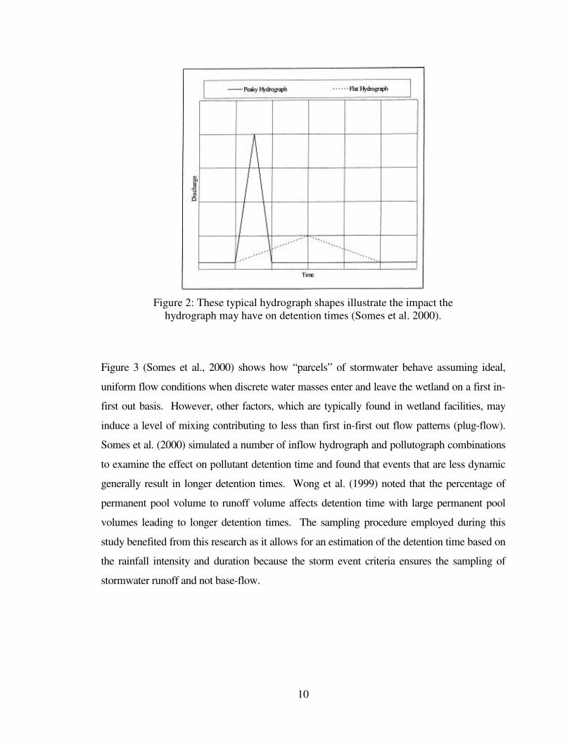
Figure 2: These typical hydrograph shapes illustrate the impact the hydrograph may have on detention times (Somes et al. 2000).
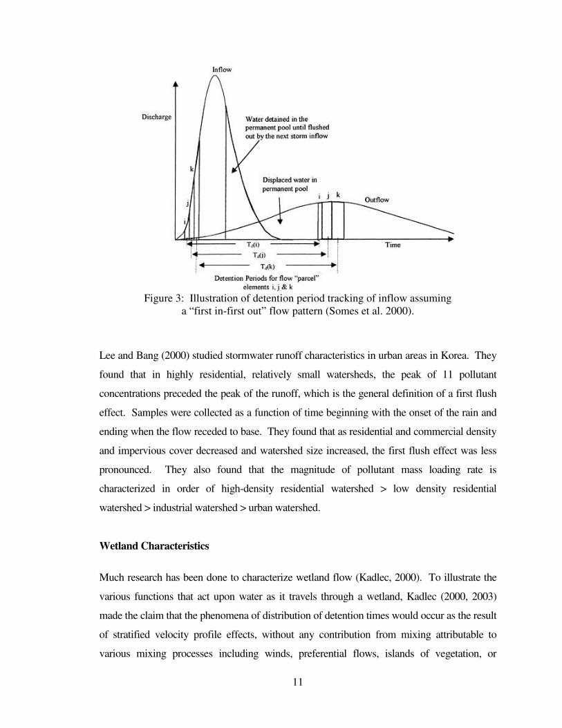
Figure 3 (Somes et al., 2000) shows how “parcels” of stormwater behave assuming ideal,
uniform flow conditions when discrete water masses enter and leave the wetland on a first in-
first out basis. However, other factors, which are typically found in wetland facilities, may
induce a level of mixing contributing to less than first in-first out flow patterns (plug-flow).
Somes et al. (2000) simulated a number of inflow hydrograph and pollutograph combinations
to examine the effect on pollutant detention time and found that events that are less dynamic
generally result in longer detention times. Wong et al. (1999) noted that the percentage of
permanent pool volume to runoff volume affects detention time with large permanent pool
volumes leading to longer detention times. The sampling procedure employed during this
study benefited from this research as it allows for an estimation of the detention time based on
the rainfall intensity and duration because the storm event criteria ensures the sampling of
stormwater runoff and not base-flow.
11
Figure 3: Illustration of detention period tracking of inflow assuming a “first in-first out” flow pattern (Somes et al. 2000).
Lee and Bang (2000) studied stormwater runoff characteristics in urban areas in Korea. They
found that in highly residential, relatively small watersheds, the peak of 11 pollutant
concentrations preceded the peak of the runoff, which is the general definition of a first flush
effect. Samples were collected as a function of time beginning with the onset of the rain and
ending when the flow receded to base. They found that as residential and commercial density
and impervious cover decreased and watershed size increased, the first flush effect was less
pronounced. They also found that the magnitude of pollutant mass loading rate is
characterized in order of high-density residential watershed > low density residential
watershed > industrial watershed > urban watershed.
Wetland Characteristics
Much research has been done to characterize wetland flow (Kadlec, 2000). To illustrate the
various functions that act upon water as it travels through a wetland, Kadlec (2000, 2003)
made the claim that the phenomena of distribution of detention times would occur as the result
of stratified velocity profile effects, without any contribution from mixing attributable to
various mixing processes including winds, preferential flows, islands of vegetation, or
12
variations of the topography, but he did not elaborate on this claim. A slug injection (one time
introduction) of a tracer dye into the influent typically produces a delayed, skewed bell-shape
curve effluent concentration of dye when plotted as a function of time (Turner Designs,
2004a)
Kadlec (1994) slug injected dye into the inlet of a wetland. To ensure maximum mixing, the
dye was poured into turbulent flow. Injecting a tracer into the wetland inlet and then
measuring the tracer concentration as a function of time at the wetland outlet is a tool used to
measure the residence time distribution. Kadlec (1994) concluded that the detention time of
the studied wetland was intermediate between plug flow and completely mixed (ideal mixing
pattern limits of water movement). The nominal detention time calculated from wetland
volume and average flow (also called the detention time) can vary from that based on dynamic
tracer studies (which are influenced by wetland functions such as sorption to wetland
particulate materials and mixing) and flow measurements by as much as 50 percent (Kadlec,
1994). The seasonal variance of wetland vegetation is one of the variables that affect the
volume of the wetland. Kadlec (1994) cites a study performed with RWT in a free water
surface wetland that showed a peak dye concentration time equal to 67% of the mean dye
detention time. This variance may be attributed to the space occupied by stems and litter as
well as to wetland zones that do not mix with the main flow. This evidence justifies using an
event-driven residence time factor to ensure the comparison of a parcel of stormwater at the
influent with the same parcel at the effluent, thus accounting for the variable nature of each
event rather than relying on calculated detention times based on the engineering design.
The state of vegetative cover affects the pollution removal potential of a constructed wetland
treating domestic wastewater. Karathanasis et al. (2003) found that the average removal of
total suspended solids (TSS) was significantly higher in vegetated systems than in unplanted
systems. This removal of TSS was noted in all seasons. This information confirms that TSS
removal is mostly a physical process involving filtration and settling. Yet, in cases where a
high percentage of TSS is organic, systems that promote microbial activity can improve
removal efficiency.
13
Shilton et al. (2000) stated, “The performance of wastewater stabilization ponds is essentially
dependant on two broad factors: the rate of reaction of the stabilizing mechanisms within the
pond environment and the time the wastewater spends in the pond environment.” The rate of
reaction of the stabilizing mechanisms is specific to conditions such as temperature and
particle size, and the time spent in the pond environment can impact settling and biotic
metabolism. Because treatment performance in a wetland depends upon the same two broad
factors, these findings are relevant here. Shilton et al. (2000) performed two studies to
compare hydraulic detention time distribution in a wastewater stabilization pond. The data
showed the concentration of dye exiting the pond was similar for both studies, displaying a
rapid rise to a peak followed by a long tail. This is typical of short–circuiting. The study
demonstrated that much of the BOD and over half the coliforms discharged untreated come
from the early part of the curves because of the effect of short-circuiting on the water through
the system and the resultant shortened treatment time. The intermittent nature of the flow rate
to the stabilization pond made it difficult to repeat the hydraulic detention time distribution.
Shilton et al. (2000) concluded that a retrofit that could delay peak discharge would
dramatically reduce the discharge of untreated coliforms.
Seaman (1956) ran a radiotracer through a settling basin three times in an attempt to determine
the detention time. For the first attempt he divided the tracer into four parts and injected them
simultaneously into four influent ports of the basin. The radioactivity of the sample taken at
three of four effluent ports was so varied that only a slight indication of the detention time was
possible. For the second run the entire radioactivity was injected into the center influent port.
For this run the background level of radiation varied and had to be subtracted from the count
of the samples pulled from the four effluent ports. The detention time was determined to be
three to four hours at two of the four effluent ports with a “high degree of confidence”
(Seaman, 1956). On the third run a different tracer was used and background level of
radiation remained constant. The detention time of an increment of effluent from the inlet to
the outlet of the settling lagoon was determined at all four effluent ports. This detention time
ranged from two hours to five hours. The experimenters varied their procedure three times
until they were convinced they had determined the detention time. This experiment illustrates
14
the difficulty of determining the detention time of even a relatively small, structurally simple
facility.
Bishop et al. (1993) used a tracer to study two drinking water clear well basins with the intent
of assessing detention time. They were able to construct a model that correlated well with the
full-scale performance. With this model they were able to add baffles to simulate optimal
configurations such as length to width ratios, inlet-outlet locations, and depth fluctuations.
Both slug and step dosage tests were useful in this study. The step-dose method entails
introduction of a tracer at a constant dosage until the concentration at the desired endpoint
reaches a steady-state level.
Sampling Methods
Harmel et al. (2003) point out that a sampling strategy which utilizes an automatic sampler
and sets a high minimum flow threshold will reduce the number of samples taken, which will
increase the difference (variability) between the measured and the true pollution flux of the
storm water runoff by increasing the effect of sample error. Grab sampling taken at a single
intake point in a stream is a generally valid representation of the water quality in the stream
because of the well-mixed conditions during storm events. This is of concern for the effluent
sampling also. Harmel et al. (2003) also emphasize the need to develop a sampling strategy
that can satisfy project goals, such as evaluating water quality improvement following
implementation of best management strategies or another goal. Implementing a sampling
protocol using a tracer dye to determine detention time for each event assures comparing the
same parcel of water at both the influent and effluent of the structure and attributes any water
quality variation to the wetland treatment system.
Turner Designs (2004a) noted that severe cases of sorption of RWT on the streambed (typical
of shallow, fine sediment) resulted in no plateau being found for studies that used constant-rate
injection (step-dose). With slug injection, a correction factor or several downstream sampling
points must be used to account for sorption. Dye may be lost due to the settling of solids.
When a fluorometer and RWT dye have been used to perform flow rate studies on surface
15
water, these calculations can be complicated by non-uniform dispersion (Turner Designs,
2004a)
Properties of Rhodamine WT & General Fluorometric Procedures for Dye Tracing
Rhodamine WT is recommended for use in water tracing because it is (1) water soluble, (2)
highly detectable – strongly fluorescent, (3) fluorescent in a part of the spectrum not common
to materials generally found in water, thereby reducing the problem of background
fluorescence, (4) harmless in low concentrations, (5) inexpensive, and (6) reasonably stable in
a normal water environment. Potential background interferences of Rhodamine WT in a
wetland include algae, naturally occurring organics, certain minerals, man-made pollutants
such as paper and textile dyes, certain petroleum products, and laundry-detergent brighteners.
Fluorescence varies depending on temperature (a 0.86 correction factor per 10 degrees F can
be used), pH, and other physical and chemical factors such as turbidity and chlorine
concentration (Turner Designs, 2004a; Wilson et al., 1986; Richardson et al., 2004).
Fluorometric procedures have been used to investigate numerous water resources (Wilson et
al., 1986, Richardson et al. 2004). The nature of the investigation dictates dye concentration,
dosing and sampling procedures, and data analysis with each application. The appropriateness
of the use of RWT in individual applications varies and should be established in advance of an
investigation (Wilson et al., 1986). RWT adsorbs to organic carbon. This could be a problem
in streams that exhibit unsteady flows with variable total organic carbon (TOC)
concentrations. Temperature and pH of the samples can be ignored if comparative raw dye
concentration data are used and the temperature variation during the event is negligible.
Fluorescence of RWT is stable over a pH range of 5-10. Fluorescence varies directly with dye
concentration.
RWT was determined to be a reliable tracer for wetlands systems that have a residence time of
less than one week, are about 0.6 m deep, and have limited sediment contact (Yu-Chen et al.,
2003). In a pilot test, RWT and a bromide tracer produced breakthrough curves that were
similar. In a full-scale test of an open surface water wetland that received flow diverted from
the Santa Ana River in California, RWT was used to calculate the mean residence time as 60
16
hours compared to the theoretical time of 69 hours. The underestimation was concluded to be
the result of RWT mass loss due to sorption through a shallow section of the system where
sediment contact is more intense (Yu-Chen et al., 2003; Jones and Jung, 1990).
Richardson et al. (2004) assessed the applicability of RWT to characterize wastewater
flow through a marshland upwelling system in a coastal setting. They selected RWT
based on research that determined it had limited toxicity to microbial populations which
are important in the treatment of soluble wastewater constituents such as carbonaceous
biochemical oxygen demand, nitrogen, and phosphorous which undergo biochemical
transformation. They reported that RWT would underestimate the actual transport
potential of the wastewater plume because the RWT tends to separate from the freshwater
zone sooner as the salinity increases. RWT did separate from the fresh water it was
injected with in response to variable salinities encountered in a two-dimensional
laboratory study described by Richardson et al. (2004). The RWT behaved differently
than the fresh water based on some chemical characteristic that mimicked sorption
behavior and allowed it to migrate through the plume at a different rate. In time,
evidence of desorption from the saline water was noted. Ghanem et al. (2003) noted the
existence of a two-step breakthrough curve for RWT typical of the multiple isomers
present in its molecular structure. Soerens et al. (2000) were able to detect and estimate
the concentration of tetrachloroethylene (PCE) in groundwater using RWT. The study
performed by Richardson et al. (2004) illustrated the potential for the RWT to migrate
through a medium at a rate different from other constituents of the influent. Soerens et al.
(2000) used five different dyes to characterize dense non-aqueous phase liquids and
found that RWT behaved differently in the presence of PCE than it did in the absence of
PCE. RWT consists of two isomers with different sorption properties in groundwater
field tests (Sutton and Kabala, 2000). This could account for the resulting two peaks
obtained in field tracer tests as seen by Richardson et al. (2004)
17
CHAPTER III
METHODOLOGY
Water Quality Analysis
Water quality was analyzed for 5-day biochemical oxygen demand (BOD5), chemical oxygen
demand (COD), total cadmium, total copper, total lead, total zinc, nitrate and nitrite nitrogen,
ammonia and Kjeldahl nitrogen, oil and grease, total and dissolved phosphorus, total dissolved
solids and total suspended solids. Samples were analyzed by the City of Tulsa Quality
Assurance Laboratory using USEPA methods or the equivalent (Appendix B). Some data sets
contain values given as “below the detection limit” (BDL) or “too numerous to count”
(TNTC>200,000). The reported detection limits vary based on the method quantification limit
of the analyzing laboratory (City of Tulsa, 2004). For calculations, BDL data are recorded as
the detection limit and TNTC>200,000 as 200,000.
Sampling Procedures for Water Quality
Samples were collected with a stainless steel bucket at the influent structure just prior to dye
introduction. Effluent samples were taken from the effluent structure for the January event
and from the effluent discharge pipe for subsequent events. Sampling procedures complied
with requirements for data collection and analysis contained in 40 CFR Part 136 (City of
Tulsa, 1991; ODEQ, 2003). Storm event criteria and sampling protocol for collecting the
influent samples assured sampling of stormwater (City of Tulsa, 1991; ODEQ, 2003).
Rainfall totaling 0.10 inch within two hours is required to identify the start of a storm event.
The runoff samples entering the wetland were collected within two hours of the start of each
event. Precipitation was measured using a rain gauge located just south of the wetland
(Appendix A).
18
Sampling Procedures for Dye Testing
All samples taken during the event and those taken during the interval between events were
analyzed for fluorescence using a Turner Designs Model 10-AU-005 Field Fluorometer,
equipped for RWT (low algae level) application with a Clear Quartz lamp 546 nm Excitation
Filter and <570 nm Emission Filter. The far-UV lamp emits a “green line” at 546 nm, which
is close to the peak excitation wavelength of RWT (Wilson et al. 1986). The same cuvette
was used throughout the study. The fluorometer was set for automatic selection of sensitivity.
A 12-volt marine battery was used as the power source (recharged between events). Raw
fluorescence data from the meter display were used to measure differences in the fluorescence
(equivalent to relative dye concentrations) between one sample and another. Wetland water
and a blank composed of deionized water were analyzed periodically during the study period
and served as assurance that the fluorometer was functioning properly through the entire
study.
Fluorometer readings are relative values of the fluorescence intensity and they alone will be
used to differentiate the relative fluorescence of each sample taken. No flow calculations will
be required and no mass balance (other than approximate) will be attempted, hence no
correction factor to account for the potential loss of dye will be used. The tracer tests were
conducted with RWT dye (Cole-Parmer). Standard solutions of RWT dye at concentrations
of 100 ppb and 50 ppb were made from water collected from Heatherridge and were used to
calibrate the fluorometer from the limit of detectability (about 10 parts per trillion) to about 0.1
ppm (Turner Designs, 1993). One gallon of dye was used for each event during this study.
One gallon will yield a concentration of 5 ppb at the effluent structure if a 50-year storm event
occurs, based on the design stormwater volume of a 50-year storm (120 acre-feet). Slug
dosage tests were used. The slug dosages were injected into the downstream end of the
influent structure, where turbulent flow was observed, usually into the middle of the flow to
ensure optimal mixing. The RWT was poured into a stainless steel sample bucket and then
dumped into the flow (Figure 4) as a slug.
The effluent was monitored for fluorescence using discrete analysis techniques in the field
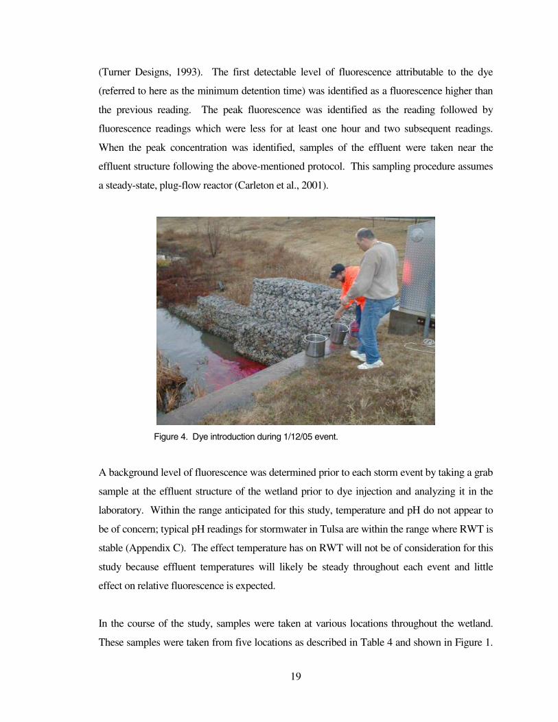
19
(Turner Designs, 1993). The first detectable level of fluorescence attributable to the dye
(referred to here as the minimum detention time) was identified as a fluorescence higher than
the previous reading. The peak fluorescence was identified as the reading followed by
fluorescence readings which were less for at least one hour and two subsequent readings.
When the peak concentration was identified, samples of the effluent were taken near the
effluent structure following the above-mentioned protocol. This sampling procedure assumes
a steady-state, plug-flow reactor (Carleton et al., 2001).
Figure 4. Dye introduction during 1/12/05 event.
A background level of fluorescence was determined prior to each storm event by taking a grab
sample at the effluent structure of the wetland prior to dye injection and analyzing it in the
laboratory. Within the range anticipated for this study, temperature and pH do not appear to
be of concern; typical pH readings for stormwater in Tulsa are within the range where RWT is
stable (Appendix C). The effect temperature has on RWT will not be of consideration for this
study because effluent temperatures will likely be steady throughout each event and little
effect on relative fluorescence is expected.
In the course of the study, samples were taken at various locations throughout the wetland.
These samples were taken from five locations as described in Table 4 and shown in Figure 1.
20
Samples were taken by reaching to dip a 500 mL bottle, attached to a two-meter pole, into the
water and then transferring to triple rinsed, 500 mL bottles. All samples were analyzed within
60 minutes of the time they were collected, minimizing the effect of any temperature change
that may exist. Samples were taken at the surface of the water. Samples were taken from
location 1 as near the point of dye injection as possible. Samples were taken from sites 2, 3
and 4 approximately three meters from the pond bank. Samples were taken from site 5
approximately one meter from the effluent riser structure in an effort to illustrate fluorescence
at this end of the facility. This monitoring may provide insight into what portion of the
wetland is involved in treating storm water. Negative readings for the de-ionized water are
relative to the fluorescence of the blank which was calibrated with pond water. At the time of
calibration, the pond water was set to zero and the standards were made using pond water.
This near weekly analysis provides evidence that the fluorometer was functioning consistently
throughout the duration of the study by assessing the steady fluorescence reading for the blank
and for any samples that had a visible fluorescence (>999). This monitoring was performed
during the intermittent period between storm events.
A t-test (alpha = 0.05) in Microsoft Excel 2000 was used to determine if a significant
difference in pollutant concentration could be found between the stormwater at the influent
and that same water tested again at the effluent.
Sampling Procedures for Subsequent Events
The effluent was sampled from the 24 inch effluent pipe for each of the events after the
January 12, 2005 event. The background level of fluorescence was determined from the
monitoring performed during the intermittent period between storm events after the January
12, 2005 event. The stage gauge data are in units of meters and do not represent the actual
depth of the wetland but show the relative depth between readings.
21
CHAPTER IV
FINDINGS
Water Quality
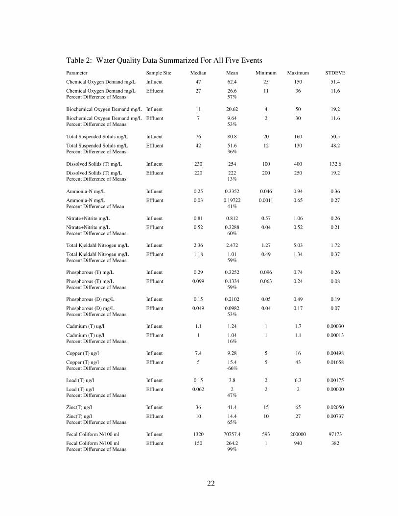
Results of the study demonstrate removal of 12 of the 14 storm water contaminants. Table 2
summarizes the data for all five events. The red numbers in Table 3 identify values recorded
as below or above the detection limit and are reported at the detection limit. The blue numbers
show the lowest value reportable based on the set-up procedure for that sample. The results
obtained for the influent and effluent sampling sites show a range of difference in contaminant
concentration from a 99% reduction for fecal coliform to –66% (negative values represent an
increase in concentration) for copper (Table 2).
A t-test was performed on the results. The average values for nitrate plus nitrite were
significantly lower at the outflow as compared to the inflow (p = 0.0045). This represents a
60% reduction. Fertilizers in urban stormwater runoff are of concern to municipal managers.
Tanner et al (2005) found removal efficiencies of 79% of nitrate/nitrite and organic nitrogen in
a constructed wetland treating drainage for grazed pasture. Kohler et al (2004) found 97%
removal of N-NO3/NO2 in a constructed wetland within a golf course during storm events.
Huett et al (2005) found that vegetated subsurface flow wetlands can remove >96% of the
nitrogen as NO3 but an unvegetated wetland removed only 16% of the nitrogen from plant
nursery runoff. Similar results were found by Shultz and Peall (2001) for removal of nitrate
during wet periods. They found removal of nitrate to be 84% compared to the same wetland
removal efficiency during dry periods of 70%. The relatively low number for the
Heatherridge facility may have been influenced by the unusually dry spring.
22
Table 2: Water Quality Data Summarized For All Five Events
Parameter Sample Site Median Mean Minimum Maximum STDEVE
Chemical Oxygen Demand mg/L Influent 47 62.4 25 150 51.4
Chemical Oxygen Demand mg/L Effluent 27 26.6 11 36 11.6Percent Difference of Means 57%
Biochemical Oxygen Demand mg/L Influent 11 20.62 4 50 19.2
Biochemical Oxygen Demand mg/L Effluent 7 9.64 2 30 11.6Percent Difference of Means 53%
Total Suspended Solids mg/L Influent 76 80.8 20 160 50.5
Total Suspended Solids mg/L Effluent 42 51.6 12 130 48.2Percent Difference of Means 36%
Dissolved Solids (T) mg/L Influent 230 254 100 400 132.6
Dissolved Solids (T) mg/L Effluent 220 222 200 250 19.2Percent Difference of Means 13%
Ammonia-N mg/L Influent 0.25 0.3352 0.046 0.94 0.36
Ammonia-N mg/L Effluent 0.03 0.19722 0.0011 0.65 0.27Percent Difference of Mean 41%
Nitrate+Nitrite mg/L Influent 0.81 0.812 0.57 1.06 0.26
Nitrate+Nitrite mg/L Effluent 0.52 0.3288 0.04 0.52 0.21Percent Difference of Means 60%
Total Kjeldahl Nitrogen mg/L Influent 2.36 2.472 1.27 5.03 1.72
Total Kjeldahl Nitrogen mg/L Effluent 1.18 1.01 0.49 1.34 0.37Percent Difference of Means 59%
Phosphorous (T) mg/L Influent 0.29 0.3252 0.096 0.74 0.26
Phosphorous (T) mg/L Effluent 0.099 0.1334 0.063 0.24 0.08Percent Difference of Means 59%
Phosphorous (D) mg/L Influent 0.15 0.2102 0.05 0.49 0.19
Phosphorous (D) mg/L Effluent 0.049 0.0982 0.04 0.17 0.07Percent Difference of Means 53%
Cadmium (T) ug/l Influent 1.1 1.24 1 1.7 0.00030
Cadmium (T) ug/l Effluent 1 1.04 1 1.1 0.00013Percent Difference of Means 16%
Copper (T) ug/l Influent 7.4 9.28 5 16 0.00498
Copper (T) ug/l Effluent 5 15.4 5 43 0.01658Percent Difference of Means -66%
Lead (T) ug/l Influent 0.15 3.8 2 6.3 0.00175
Lead (T) ug/l Effluent 0.062 2 2 2 0.00000Percent Difference of Means 47%
Zinc(T) ug/l Influent 36 41.4 15 65 0.02050
Zinc(T) ug/l Effluent 10 14.4 10 27 0.00737Percent Difference of Means 65%
Fecal Coliform N/100 ml Influent 1320 70757.4 593 200000 97173
Fecal Coliform N/100 ml Effluent 150 264.2 1 940 382Percent Difference of Means 99%
23
Table 3: 2005 Water Quality Data From Heatherridge.L
ocat
ion
Tim
e
DA
TE
Che
mic
al O
xyge
n D
eman
d m
g/L
Bio
chem
ical
Oxy
gen
Dem
and
mg/
L
Tot
al S
uspe
nded
Sol
ids
mg/
L
Dis
solv
ed S
olid
s (T
) m
g/L
Am
mon
ia-N
mg/
L
Nit
rate
+N
itri
te m
g/L
Tot
al K
jeld
ahl N
itrog
en m
g/L
Pho
spho
rous
(T
) m
g/L
Pho
spho
rous
(D
) m
g/L
Cad
miu
m (
T)
mg/
l
Cop
per
(T)
mg/
l
Lea
d (T
) m
g/l
Zin
c(T
) m
g/l
Fec
al C
olif
orm
N/1
00 m
l
pH
Har
dnes
s as
CaC
O3
mg/
L
Tem
p °C
Influent
17:00 1/12/2005 25 3.7 76 380 0.10 0.81 1.27 0.15 0.027 0.0010 0.0050 0.0023 0.032 593 8 148 13.3
Effluent
9:30 1/13/2005 25 2 60 220 0.27 0.52 1.18 0.099 0.049 0.0010 0.0050 0.0020 0.0100 150 8.2 147 7.7% removal 0 46 21 42 -170 36 7 34 -81 0 0 13 69 75
Influent
20:00 2/12/05 27 30 20 400 0.046 0.88 0.49 0.096 0.053 0.0011 0.0050 0.0020 0.015 874 7.4 312 11.1
Effluent
7:00 2/5/2005 13 30 12 250 0.030 0.17 0.47 0.063 0.062 0.0011 0.0050 0.0020 0.010 78 7.5 191 12.5% removal 52 0 40 38 35 81 4 34 -17 0 0 0 33 91
Influent
4:00 3/21/2005 47 8.4 160 230 0.25 0.40 2.43 0.29 0.088 0.0017 0.0074 0.00390 0.036 1320 7.8 218 12.4
Effluent
14:15 3/21/2005 11 3 14 230 0.030 0.040 0.78 0.075 0.040 0.0013 0.0050 0.0020 0.010 940 7.8 156 13.6% removal 77 64 91 0 88 90 68 74 55 24 32 49 72 29
Influent
21:20 4/25/2005 150 50.0 82 160 0.94 1.06 5.03 0.74 0.49 0.0010 0.013 0.00450 0.059 200000 7.6 156 16.2
Effluent
13:00 4/28/2005 36 6.7 130 200 0.65 0.040 1.26 0.24 0.17 0.0010 0.043 0.0020 0.015 1 8.8 170 23% removal 76 87 -59 -25 31 96 75 68 65 0 -231 56 75 100
Influent
23:15 5/13/2005 65 11 66 100 0.34 0.57 2.36 0.35 0.15 0.0014 0.016 0.00630 0.065 151000 7.4 53.7 21.4
Effluent
6:00 5/14/2005 34 6.5 42 210 0.035 0.044 1.34 0.19 0.17 0.0010 0.019 0.0020 0.027 153 8.7 118 21.4% removal 48 41 36 -110 90 92 43 46 -13 29 -19 68 58 100
24
Fecal coliform concentrations percent difference of means is 99.6%. They ranged from as
high as TNTC>200,000 (Too Numerous To Count) CFU / 100 ml at the influent to <1 CFU /
100 ml at the effluent for the 4/25/2005 event (reported in the data as 200,000 and 1
respectively). The comparison between the two locations (influent and effluent) shows that
there is no significant difference (p=0.14344) due to the variability.
The removal difference can be compared to bacterial removal of 90% from domestic
wastewater by both planted and unplanted pilot scale constructed wetlands (Keffala and
Ghrabi, 2005). Song et al. (2006) found removal efficiencies for fecal coliform similar to
other municipal treatment wetlands of 99.6%. These data compared samples gathered from a
constructed wetland inlet structure that was downstream from a primary settling basin to
samples gathered from the effluent. The bacteria that entered the wetland were likely
adsorbed to fine sediment and as such afforded little protection from biological agents.
A contaminant of concern in urban runoff is phosphorus from fertilizer. Huett et al (2005)
found that planted wetland tubs can remove 88% P (as PO4, the dominant species in plant
nursery runoff) whereas unplanted tubs removed only 45% percent. Plant uptake was found
to be the dominant removal mechanism in reducing total phosphorus. Song et al. (2006)
found that phosphorus removal efficiencies exhibited seasonal variations. Total phosphorus
removal was more efficient in the summer and fall. A seasonal monitoring regimen may
discover re-suspension of phosphorus during high flow events.
The percent reductions for total and dissolved phosphorus were 59 and 53 respectively in this
study (Table 2). The average values were not significantly lower at the outflow as compared
to the inflow. Heatherridge performance can be compared to stormwater treatment area
wetlands with either emergent aquatic vegetation or submerged aquatic vegetation constructed
by the South Florida Water Management District (Juston and DeBusk 2005). Two to seven
years of data indicated phosphorus mass removal efficiencies consistently above 85% adjusted
for background contaminant concentration, with mass loading rates at or below 2g/m2•yr.
25
Total P mass reduction of 59% (Kao and Wu, 2001) has been reported as stormwater passed
through a natural wetland, comparable to results in this study. Kohler et al (2004) found
phosphorus removal of 74% during storm events for a constructed wetland treating golf course
runoff. This may be the result of fewer toxics entering the wetland than would be the case
with runoff associated with a mixed-use urban watershed.
This study showed a 51% difference in influent to effluent for Kjeldahl nitrogen (Table 2).
Though not significantly different, it can be compared to Kjeldahl nitrogen percent removal in
a planted and an unplanted system of 27 and 5% respectively (Keffala and Ghrabi 2005).
Total suspended solids and total dissolved solids are generally agreed to be physical
contaminants of concern for municipal stormwater managers. Heatherridge removal
differences were 26% and –11% respectively (Table 4). The Heatherridge facility did not
show a significant removal of either of these contaminants. One reason for the poor
performance of the dissolved solids may be the relatively short duration of the detention time
(6.75 hours) before the 5/13/05 event that did not allow for prolonged treatment. It appears
counterintuitive that the longest detention time of 66 hours for the 4/21/05 event results in an
increase of 59% total suspended solids.
Dye Testing
The average elapsed time from the time the dye was injected into the stormwater runoff at the
influent structure until the time fluorescence was first detected at the outfall (the estimated
minimum detention time) was 20.4 hours with a standard deviation of 24.1 hours for all
sampling events. The 4/25/05 event accounted for the majority of the variability. The
estimated average time to peak (most representative of the stormwater collected and analyzed
at the influent) was 21.6 hours with a standard deviation of 23.8 hours.
The range of stage gage readings was 5.3 meters on 2/18 to 2.7 meters on 5/4/05 (Table 4).
The lowering of the permanent pool through the duration of the study provides evidence of a
dry spring.
26
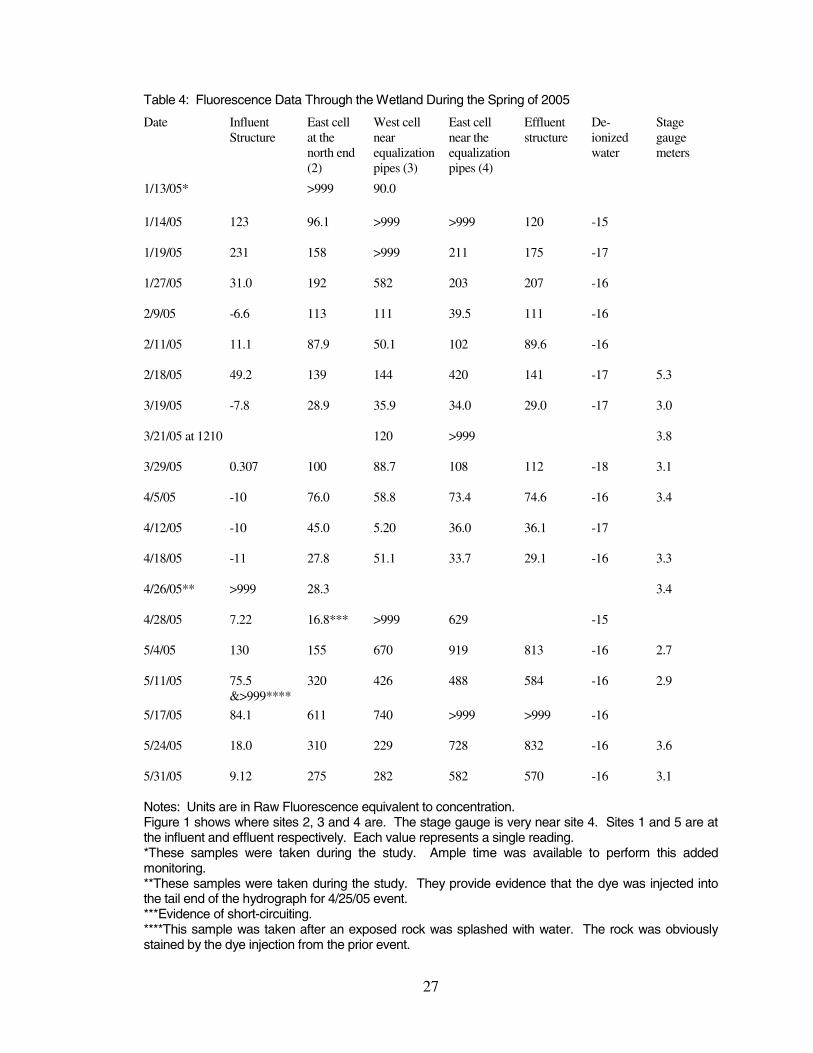
Table 4 and Figure 5 summarize the background fluorescence through the wetland. The >999
readings are above the maximum allowable for the screen. For the purposes of this study, it
need only be understood that there is enough fluorescence present to be visible to the eye. The
sample from the north end of the east cell on 4/28/05 shows that the dye did not reach this end
of the facility. These data provide evidence of short-circuiting and/or preferential flow
patterns because the fluorescence of the sample did not appear to be influenced by the
presence of dye. More could be learned from this measure if a detailed relationship could be
made with the permanent pool volume. Additional monitoring sites would provide evidence
of flow path.
Figure 5 illustrates the impact of the rainfall intensity on the flow of dye through the wetland.
Rainfall totaled 0.2 inches in six minutes for the 4/25/05 storm event and the dye was
introduced one hour and 13 minutes after the rain ended. The high fluorescence at the influent
structure on 4/26/05 indicates the dye was added to the tail end of the hydrograph. The
readings at sites 3 and 4 and at the effluent from 5/4 to 5/11/2005 indicate the dye lingered in
the wetland until the 5/13/2005 rainfall caused it to be “pushed out”.
0
100
200
300
400
500
600
700
800
900
1000
1/13/2005 1/23/2005 2/2/2005 2/12/2005 2/22/2005 3/4/2005 3/14/2005 3/24/2005 4/3/2005 4/13/2005 4/23/2005 5/3/2005 5/13/2005 5/23/2005
Date
Raw
Flu
ores
cenc
e
Influent structureEast cell at the north end (2)West cell near equalization pipes (3)East cell near the equalization pipes (4)Effluent structure
Figure 5. Fluorescence in wetland during study.
The data for the 5/13/05 event during this study (Figure 11), likely mimic the phenomenon of
water detained in the permanent pool (Figure 3) due to low rainfall volume for the prior event
and the relatively short (19 day) interval between events.
27
Notes: Units are in Raw Fluorescence equivalent to concentration.Figure 1 shows where sites 2, 3 and 4 are. The stage gauge is very near site 4. Sites 1 and 5 are at the influent and effluent respectively. Each value represents a single reading.*These samples were taken during the study. Ample time was available to perform this added monitoring.**These samples were taken during the study. They provide evidence that the dye was injected into the tail end of the hydrograph for 4/25/05 event.***Evidence of short-circuiting.****This sample was taken after an exposed rock was splashed with water. The rock was obviously stained by the dye injection from the prior event.
Table 4: Fluorescence Data Through the Wetland During the Spring of 2005
Date Influent Structure
East cell at the north end (2)
West cell near equalization pipes (3)
East cell near the equalization pipes (4)
Effluent structure
De-ionized water
Stage gaugemeters
1/13/05* >999 90.0
1/14/05 123 96.1 >999 >999 120 -15
1/19/05 231 158 >999 211 175 -17
1/27/05 31.0 192 582 203 207 -16
2/9/05 -6.6 113 111 39.5 111 -16
2/11/05 11.1 87.9 50.1 102 89.6 -16
2/18/05 49.2 139 144 420 141 -17 5.3
3/19/05 -7.8 28.9 35.9 34.0 29.0 -17 3.0
3/21/05 at 1210 120 >999 3.8
3/29/05 0.307 100 88.7 108 112 -18 3.1
4/5/05 -10 76.0 58.8 73.4 74.6 -16 3.4
4/12/05 -10 45.0 5.20 36.0 36.1 -17
4/18/05 -11 27.8 51.1 33.7 29.1 -16 3.3
4/26/05** >999 28.3 3.4
4/28/05 7.22 16.8*** >999 629 -15
5/4/05 130 155 670 919 813 -16 2.7
5/11/05 75.5 &>999****
320 426 488 584 -16 2.9
5/17/05 84.1 611 740 >999 >999 -16
5/24/05 18.0 310 229 728 832 -16 3.6
5/31/05 9.12 275 282 582 570 -16 3.1
28
Observations of the 1/12/05 Event
On 1/12/05, 0.12 inches of rain fell from 1550 to 1637, and then the rain stopped. Influent
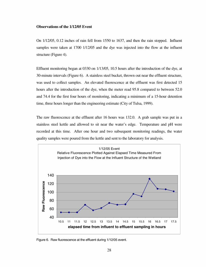
samples were taken at 1700 1/12/05 and the dye was injected into the flow at the influent
structure (Figure 4).
Effluent monitoring began at 0330 on 1/13/05, 10.5 hours after the introduction of the dye, at
30-minute intervals (Figure 6). A stainless steel bucket, thrown out near the effluent structure,
was used to collect samples. An elevated fluorescence at the effluent was first detected 15
hours after the introduction of the dye, when the meter read 95.8 compared to between 52.0
and 74.4 for the first four hours of monitoring, indicating a minimum of a 15-hour detention
time, three hours longer than the engineering estimate (City of Tulsa, 1999).
The raw fluorescence at the effluent after 16 hours was 132.0. A grab sample was put in a
stainless steel kettle and allowed to sit near the water’s edge. Temperature and pH were
recorded at this time. After one hour and two subsequent monitoring readings, the water
quality samples were poured from the kettle and sent to the laboratory for analysis.
1/12/05 EventRelative Fluorescence Plotted Against Elapsed Time Measured From Injection of Dye into the Flow at the Influent Structure of the Wetland
40
60
80
100
120
140
10.5 11 11.5 12 12.5 13 13.5 14 14.5 15 15.5 16 16.5 17 17.5
elapsed time from influent to effluent sampling in hours
Raw
Flu
ore
scen
ce
Figure 6. Raw fluorescence at the effluent during 1/12/05 event.
29
The tracer response during the first event displayed a detention period for the dye of at least 15
hours. The peak of the distributed dye detention period was estimated to be 16 hours. On
1/19/05 at 1000 a sample taken from the west cell (site 3) read >999 and one at the effluent
read 175. This monitoring provides evidence that the effluent sample collected and analyzed
on 1/13/05 did not account for all of the dye added.
Observations of the 2/12/05 Event
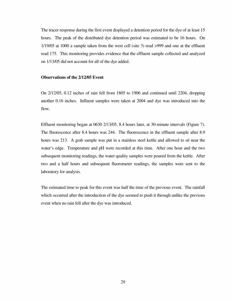
On 2/12/05, 0.12 inches of rain fell from 1805 to 1906 and continued until 2204, dropping
another 0.16 inches. Influent samples were taken at 2004 and dye was introduced into the
flow.
Effluent monitoring began at 0630 2/13/05, 8.4 hours later, at 30-minute intervals (Figure 7).
The fluorescence after 8.4 hours was 244. The fluorescence in the effluent sample after 8.9
hours was 213. A grab sample was put in a stainless steel kettle and allowed to sit near the
water’s edge. Temperature and pH were recorded at this time. After one hour and the two
subsequent monitoring readings, the water quality samples were poured from the kettle. After
two and a half hours and subsequent fluorometer readings, the samples were sent to the
laboratory for analysis.
The estimated time to peak for this event was half the time of the previous event. The rainfall
which occurred after the introduction of the dye seemed to push it through unlike the previous
event when no rain fell after the dye was introduced.
30
2/12/05 EventRelative Fluorescence Plotted Against Elapsed Time Measured From
Injection
180
190
200
210
220
230
240
250
8.4 9 9.4 10 10.4 11 11.4
elapsed time from influent to effluent sampling in hours
Raw
Flu
ore
scen
ce
Figure 7. Raw fluorescence at the effluent during 2/12/05 event.
A sample from the west cell (site 4) taken 2/13/05 approximately nine hours after the dye was
injected had a noticeable red tint to it and a fluorescence reading of >999.
On 2/18/05 at 1400 monitoring was performed at the identified background fluorescence sites
(Table 4). The fluorescence at site 4 and the effluent, 420, and 141 respectively, provides
evidence that the dye was on its way out by then because the fluorescence at both sites was
less than it was on 2/13/05. No adjustment to the effluent sampling protocol was made. The
estimated minimum detention time for this event was less than eight and one half hours, one
and one half hours less than the engineering estimate (City of Tulsa, 1999).
Observations of the 3/21/05 Event
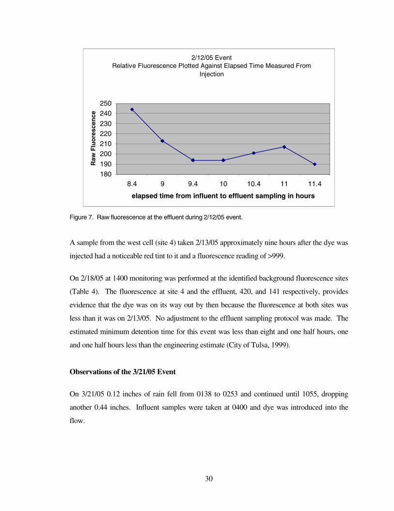
On 3/21/05 0.12 inches of rain fell from 0138 to 0253 and continued until 1055, dropping
another 0.44 inches. Influent samples were taken at 0400 and dye was introduced into the
flow.
31
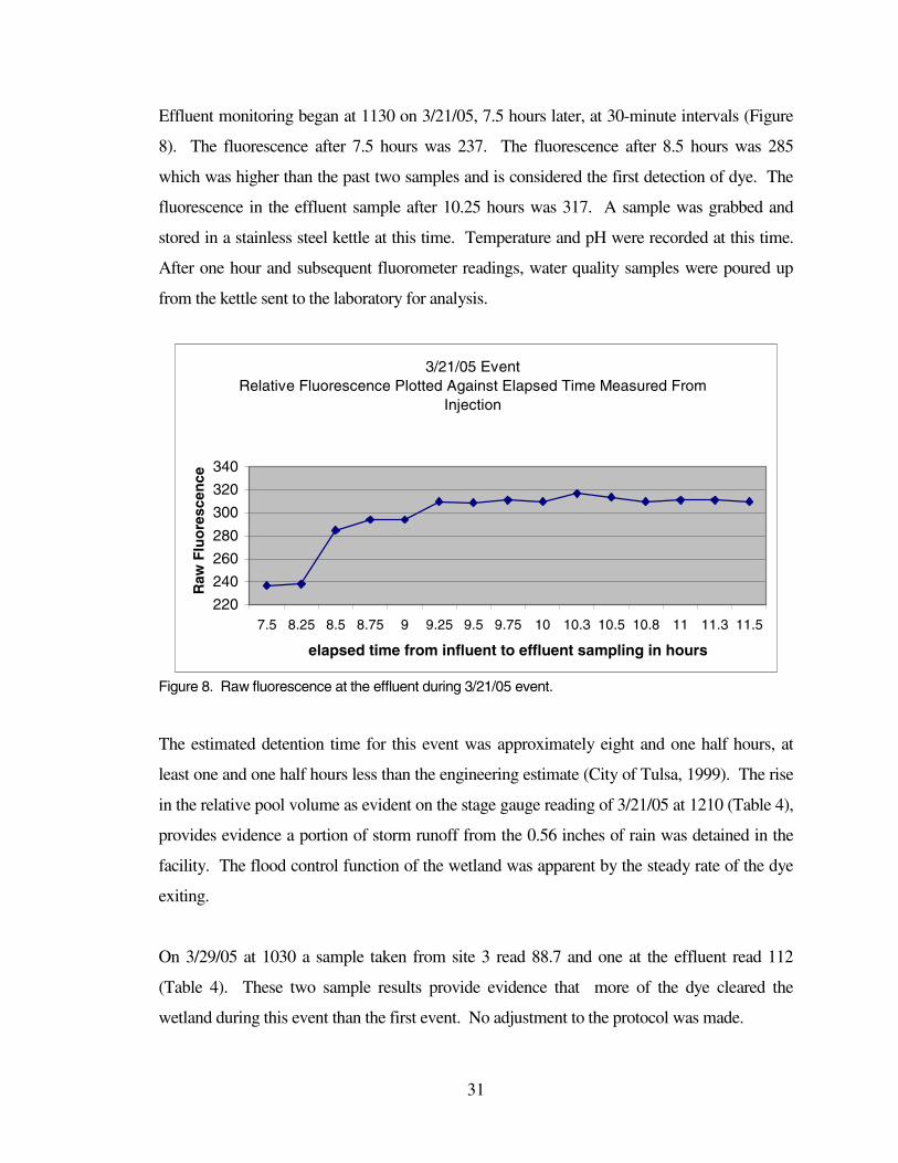
Effluent monitoring began at 1130 on 3/21/05, 7.5 hours later, at 30-minute intervals (Figure
8). The fluorescence after 7.5 hours was 237. The fluorescence after 8.5 hours was 285
which was higher than the past two samples and is considered the first detection of dye. The
fluorescence in the effluent sample after 10.25 hours was 317. A sample was grabbed and
stored in a stainless steel kettle at this time. Temperature and pH were recorded at this time.
After one hour and subsequent fluorometer readings, water quality samples were poured up
from the kettle sent to the laboratory for analysis.
3/21/05 EventRelative Fluorescence Plotted Against Elapsed Time Measured From
Injection
220
240
260
280
300
320
340
7.5 8.25 8.5 8.75 9 9.25 9.5 9.75 10 10.3 10.5 10.8 11 11.3 11.5
elapsed time from influent to effluent sampling in hours
Raw
Flu
ore
scen
ce
Figure 8. Raw fluorescence at the effluent during 3/21/05 event.
The estimated detention time for this event was approximately eight and one half hours, at
least one and one half hours less than the engineering estimate (City of Tulsa, 1999). The rise
in the relative pool volume as evident on the stage gauge reading of 3/21/05 at 1210 (Table 4),
provides evidence a portion of storm runoff from the 0.56 inches of rain was detained in the
facility. The flood control function of the wetland was apparent by the steady rate of the dye
exiting.
On 3/29/05 at 1030 a sample taken from site 3 read 88.7 and one at the effluent read 112
(Table 4). These two sample results provide evidence that more of the dye cleared the
wetland during this event than the first event. No adjustment to the protocol was made.
32
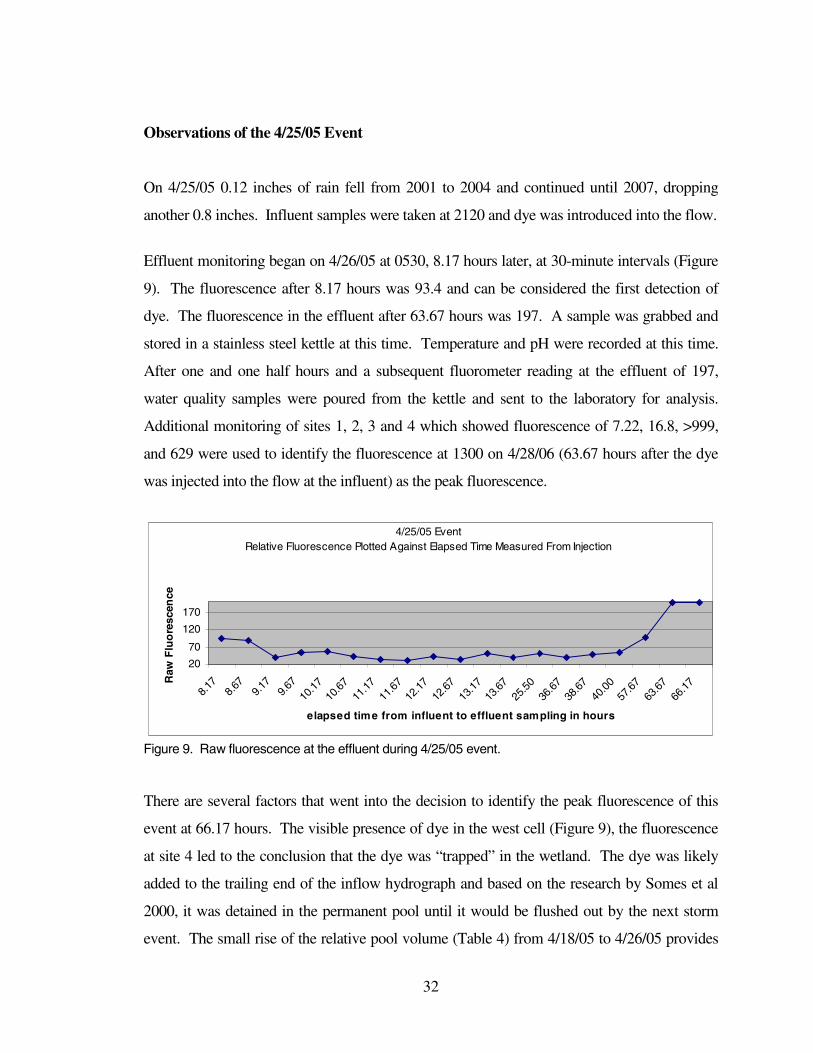
Observations of the 4/25/05 Event
On 4/25/05 0.12 inches of rain fell from 2001 to 2004 and continued until 2007, dropping
another 0.8 inches. Influent samples were taken at 2120 and dye was introduced into the flow.
Effluent monitoring began on 4/26/05 at 0530, 8.17 hours later, at 30-minute intervals (Figure
9). The fluorescence after 8.17 hours was 93.4 and can be considered the first detection of
dye. The fluorescence in the effluent after 63.67 hours was 197. A sample was grabbed and
stored in a stainless steel kettle at this time. Temperature and pH were recorded at this time.
After one and one half hours and a subsequent fluorometer reading at the effluent of 197,
water quality samples were poured from the kettle and sent to the laboratory for analysis.
Additional monitoring of sites 1, 2, 3 and 4 which showed fluorescence of 7.22, 16.8, >999,
and 629 were used to identify the fluorescence at 1300 on 4/28/06 (63.67 hours after the dye
was injected into the flow at the influent) as the peak fluorescence.
4/25/05 EventRelative Fluorescence Plotted Against Elapsed Time Measured From Injection
20
70
120
170
8.17
8.67
9.17
9.67
10.1
710
.67
11.1
711
.67
12.1
712
.67
13.1
713
.67
25.5
036
.67
38.6
740
.00
57.6
763
.67
66.1
7
elapsed time from influent to effluent sampling in hours
Raw
Flu
ore
scen
ce
Figure 9. Raw fluorescence at the effluent during 4/25/05 event.
There are several factors that went into the decision to identify the peak fluorescence of this
event at 66.17 hours. The visible presence of dye in the west cell (Figure 9), the fluorescence
at site 4 led to the conclusion that the dye was “trapped” in the wetland. The dye was likely
added to the trailing end of the inflow hydrograph and based on the research by Somes et al
2000, it was detained in the permanent pool until it would be flushed out by the next storm
event. The small rise of the relative pool volume (Table 4) from 4/18/05 to 4/26/05 provides
33
evidence the small rainfall volume and short duration had little impact on the facility and is
consistent with an extended detention time of the runoff.
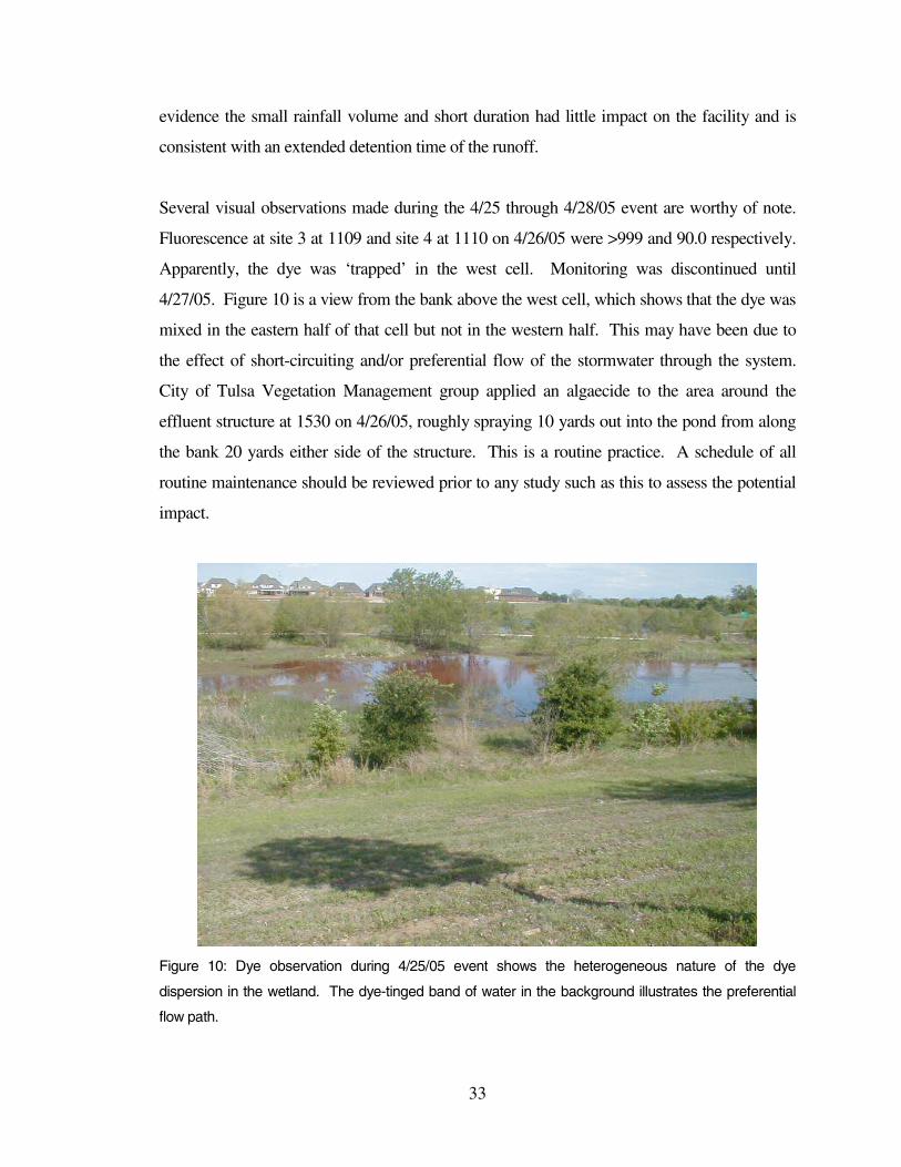
Several visual observations made during the 4/25 through 4/28/05 event are worthy of note.
Fluorescence at site 3 at 1109 and site 4 at 1110 on 4/26/05 were >999 and 90.0 respectively.
Apparently, the dye was ‘trapped’ in the west cell. Monitoring was discontinued until
4/27/05. Figure 10 is a view from the bank above the west cell, which shows that the dye was
mixed in the eastern half of that cell but not in the western half. This may have been due to
the effect of short-circuiting and/or preferential flow of the stormwater through the system.
City of Tulsa Vegetation Management group applied an algaecide to the area around the
effluent structure at 1530 on 4/26/05, roughly spraying 10 yards out into the pond from along
the bank 20 yards either side of the structure. This is a routine practice. A schedule of all
routine maintenance should be reviewed prior to any study such as this to assess the potential
impact.
Figure 10: Dye observation during 4/25/05 event shows the heterogeneous nature of the dye
dispersion in the wetland. The dye-tinged band of water in the background illustrates the preferential
flow path.
34
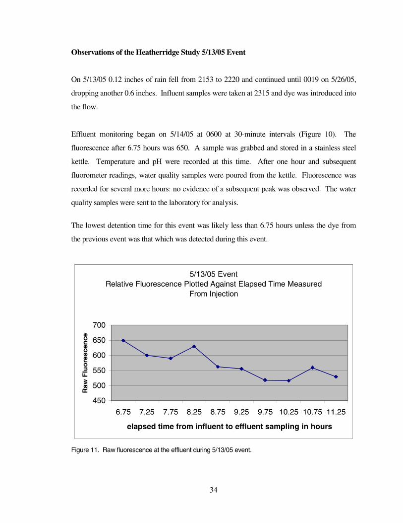
Observations of the Heatherridge Study 5/13/05 Event
On 5/13/05 0.12 inches of rain fell from 2153 to 2220 and continued until 0019 on 5/26/05,
dropping another 0.6 inches. Influent samples were taken at 2315 and dye was introduced into
the flow.
Effluent monitoring began on 5/14/05 at 0600 at 30-minute intervals (Figure 10). The
fluorescence after 6.75 hours was 650. A sample was grabbed and stored in a stainless steel
kettle. Temperature and pH were recorded at this time. After one hour and subsequent
fluorometer readings, water quality samples were poured from the kettle. Fluorescence was
recorded for several more hours: no evidence of a subsequent peak was observed. The water
quality samples were sent to the laboratory for analysis.
The lowest detention time for this event was likely less than 6.75 hours unless the dye from
the previous event was that which was detected during this event.
5/13/05 EventRelative Fluorescence Plotted Against Elapsed Time Measured
From Injection
450
500
550
600
650
700
6.75 7.25 7.75 8.25 8.75 9.25 9.75 10.25 10.75 11.25
elapsed time from influent to effluent sampling in hours
Raw
Flu
ore
scen
ce
Figure 11. Raw fluorescence at the effluent during 5/13/05 event.
35
CHAPTER V
CONCLUSION
Water Quality
Constructed wetlands are increasingly popular for storm water treatment in urban settings. It
is important to quantify the removal efficiency of these wetlands to assess their benefit and
role in an overall storm water management plan. This study addresses the stormwater
treatment efficiency of Heatherridge Stormwater Detention Facility, a constructed wetland
created specifically for the dual purpose of retaining stormwater and mitigating wetlands
impacted by construction of a highway. The City of Tulsa has added this facility to its Storm
Water Management Plan due to the potential for wetlands to treat stormwater runoff and
enhance the quality of water as it passes through the system. Results of the study demonstrate
removal of 12 of the 14 stormwater contaminants.
The average percent difference of means for the nutrient (nitrate + nitrite, total Kjeldahl
nitrogen and ammonia-N) stormwater pollutants showed reductions of 60, 59 and 41 percent
respectively. Both total and dissolved phosphorus were also reduced over the course of this
study. The reduction of these pollutants is essential to the health of the downstream section of
the stream.
Potential Retrofits
A detailed study of the Heatherridge Stormwater Detention Facility catchment area is in order
to determine if the runoff quality is in line with typical urban land uses and the time of travel
of certain pollutants. These data could provide guidance in retrofitting measures. It would be
advantageous to understand the source and nature of the TSS (and other lumped, or grouped,
parameters) entering the system to target those functions that support water quality
36
improvement (Kadlec, 2002). Retrofits that enhance settling of large particulate matter may
miss the goal of reduced pollution concentration at the effluent due to the potential of small
particulate matter having relatively greater sorption potential and longer settling rates. For a
detailed discussion of the relationship of tracer testing and its applicability to assess the
removal rates of lumped parameters see Kadlec (2002).
Dye Testing
The detention times, based on fluorescence analysis, show a distribution of estimated peak
detention times from a minimum of 8.5 hours to approximately 63.5 hours. This variation can
be attributed to rainfall intensity, duration, and time between storm events. The minimum
detention time for the 3/21/05 event was eight and one half hours (Figure 7). The stage
reading on 3/19/05 was 3.0 meters which represents the lowest level within the study period to
date. The rainfall amount for this event totaled 0.56 inches. Wong et al. (1999) observed that
small permanent pool volumes and large runoff volumes led to short detention times. The
same behavior was observed during the 3/21/05 event. The maximum detention time was not
identified during this study, but the 4/21/05 event provides evidence it could be as much as 63
hours (Figure 9). The likelihood of the dye being stuck in the wetland is high. A short,
intense, rain event and a long delay until the dye was added predict a long detention time as
modeled by Somes et al. (2000). Observations during the 4/25/05 event show that not all of
the wetland waters mix with the main flow. This observation highlights the potentially severe
impact that short-circuiting can have on treatment efficiency. Since many wetland reactions
involve sedimentation and biota that are distributed unevenly throughout the facility, it would
be advantageous to account for differential treatment potentials prior to suggesting retrofitting
techniques. It would be advantageous to monitor the mixing of dye throughout the wetland in
more detail to increase the confidence of the detention time. The use of an engineering
estimate is an unreliable predictor of the detention time for a parcel of water through this
facility due to the variable nature of rainfall in northeast Oklahoma. The data obtained by this
monitoring may provide evidence relating to background fluorescence, potential short-
circuiting or preferential flow patterns of the dye through the wetland, effective treatment
capacity of the wetland, and how long the dye remains in the system.
37
Further detail should be given to study goals in relation to possible retrofits available to utility
managers. More research is warranted with respect to lumped parameters to help choose
BMPs to address the most abundant or threatening components.
Limitations
Water Quality
The historical data were gathered under the assumption that an engineering estimate of the
detention time for the facility was 12 hours. The first indication of the origin of this estimate
was discovered in unpublished City of Tulsa internal documentation that states, in a hand-
written note, “Samples were obtained approximately 14 hours apart to compensate for
detention time.” Although the note states “14 hours apart”, the time reported in the document
records that the influent was sampled at “8:40pm 2/6/99” and the effluent was sampled at
“6:35am 2/7/99” (City of Tulsa, 1999), which is approximately 10 hours. The average
interval between influent and effluent sampling for the monitoring program referred to as the
“Heatherridge Historic Data” is 11.8 hours, which is consistent with the engineering
assumption that the detention time was 12 hours throughout previous monitoring periods. It
would be beneficial to any further monitoring at this site to account for the effect of age on the
overall volume of the facility to allow for a more accurate estimation of detention time. This
could be accomplished by mapping the depth of the wetland. This information would provide
additional evidence of potential flow patterns and the volume of the facility that affects
detention time and treatment. It would also be beneficial to assess the runoff coefficient of the
watershed to account for any development or change in land use to account for watershed
hydrology.
The seasonal impact on the functions and values of an urban water body affects the water
quality enhancement potential. Further study is warranted to account for treatment in each
season of the year.
38
Dye Testing
The sampling of the effluent during the 1/12/05 event from the area around the effluent
structure allows for variability based on where the bucket was thrown and how deep the
bucket sank into the pool, among other things. A change in the effluent monitoring site to the
24 inch effluent pipe addressed these concerns. The effluent samples for this event appeared
to identify peak fluorescence during this event.
The influent sampling during the 2/12/05 event and the effluent sampling during the 4/25/05
event exposed a limit within the peak fluorescence identification criteria, namely sampling
must begin prior to the arrival of the dye at the sampling point and continue until all traces of
dye have disappeared. Criteria must be set to identify peak fluorescence consistent with the
nature of the study. The background fluorescence monitoring of 1/14/05 of sites 2 and 3
provides evidence that the effluent sample collected and analyzed on 1/13/05 accounted for a
small fraction of the mass of dye added and may not have been the most representative parcel
of water the dye was introduced into.
Although the Model 10-AU-005 Field Fluorometer User’s Manual states that “you do not
have to calibrate every time you read a new batch of samples,” some criteria should be
identified to assure the reliability of the readings. The identification of the first detectable
level of fluorescence attributable to the dye must be defined by criteria that suits the
investigation.
The target concentration of dye was set under the assumption that the facility is new. It is
likely to be inaccurate due to a change in the wetland volume. A survey of the permanent
pool volume measurements would allow further development of the relationship of the stage
measurements taken during this study (Table 2) and may be used to better characterize the
effect of RWT sorption on the streambed.
The literature review revealed a potential background interference of Rhodamine WT in a
wetland. This study accounted for background fluorescence through periodic monitoring
39
throughout the wetland. Although no evidence of massive variability of the fluorescence
occurred during any of the monitoring, it would be prudent to set a criteria to identify any
fluorescence outside that which is expected for any given study. The impact on fluorescence
of temperature, pH, loss due to sorption, and the factors which may affect the readings and
interpretation must be addressed in the method. Thus, further study should be done to
characterize water quality of the permanent pool and account for the effect it has on the time
of travel of RWT.
Assessment Techniques and Goals
The data collected during this research project have contributed to the understanding of the
potential for a constructed wetland to perform water purification processes. Stormwater utility
managers need this type of data to make informed choices between the abundant varieties of
BMPs available for an equally large number of management goals.
A study performed by Pitt et al. (1995) found urbanization could impair beneficial uses. In an
extensive literature review, these researchers cited studies that indicated increased
urbanization correlated to decreased numbers of macroinvertibrates even if water-quality
parameters did not identify a high degree of pollution. They concluded it is near impossible,
due to all the variables and site-specific relationships between them, to predict the effect any
will have on the receiving stream based solely on water column quality measurements.
Perhaps an alternative assessment protocol, one which is inclusive of the biota and the location
in the landscape, would be able to provide insight into whether Heatherridge is a successful
water quality mitigation project. It is likely such an assessment would require an assessment
of water quality issues as well and data like that collected during this study would contribute
to the decision process. It is imperative to any wetland assessment exercise that the particular
functions or parameters to be evaluated are clearly defined (Whigham, 1999).
Whigham (1999) suggests comparing a constructed wetland with natural wetlands, often
referred to as reference wetlands, when assessing the success or failure of a system. Since
water quality enhancement is but one function of a more complex system, it may be useful to
40
study this aspect in conjunction with other important functions and values. At least with this
forethought, an efficient, tailored protocol may be developed. Hager (2004) recommends
utility managers focus resources on assessing the effectiveness of BMPs to address first flush
contaminants. This article also pointed out the site specific nature of the runoff and BMP
selection. The number of factors that must be considered is formidable.
Clear, quantitative monitoring objectives must be developed for stormwater monitoring. It is
essential that one clearly determine the criteria for a successful wetland treatment facility
while developing the water quality assessment strategy.
The assessment of any best management practice demands an understanding of the impact of
the threat prior to control. Heatherridge Wetland was designed as a flood control structure and
stormwater treatment facility to mitigate the loss of natural wetlands. It is likely an
engineering formula can assess the physical impact that urbanization will have on the
hydrology of a watershed. It is less likely that a water quality or hydrology formula can assess
a stormwater quality BMP because stormwater utility managers must assess values other than
just physical properties. Natural wetlands are credited for mitigating flooding and water
quality enhancement. Natural wetlands provide value to the urban setting. It appears
Heatherridge can successfully function as a flood control device. It is hoped that the value
Heatherridge provides will mimic a natural wetland. Further study will shed light on the
question.

41
REFERENCES
Burton, Knowles, and Love, Inc. 1991. Preliminary Design Report for Heatherridge Stormwater Detention Facility, Project No. 901025, City of Tulsa, Oklahoma.
Burton, Knowles, and Love, Inc. 1992. Final Design Report for Heatherridge Stormwater Detention Facility, Project No. 901025, City of Tulsa, Oklahoma 1992.
Bidwell, J. R. and Gorrie J. R. 1998. A survey of the Aquatic Invertebrate Community in a Constructed Wetland. In: Proceedings of the HydraStorm Conference, Adelaide, September 27-30, 1998. Institute of Engineers, Australia, ISBN 1858257122. pp 463-470.
Bishop, M.M., Morgan, J.M., Cornwell, B., Jamison, D.K. 1993. Improving the Disinfection Detention Time of a Water Plant Clearwell. Research and Technology Journal American Water Works Association, pp 68-75.
Brinson, M. 1993. A Hydrogeomorphic Classification for Wetlands. Wetlands Research Program Technical Report WRP-DE-4 U.S. Army Corps of Engineers. August 1993 – Final Report.
Carleton, J.N., Grizzard, T.J., Godrej, A.N. 2001. Factors Affecting the Performance of Stormwater Treatment Wetlands. Water Research, Volume 35, Issue 6, pp1552-1562.
Carter Burgess, Inc. 2001. Urban Watersheds, How Science and Engineering Can Manage, Protect and Preserve Urban Stream Corridors. Special Report of Technically Speaking.
City of Tulsa. 2003. The Flood Control Project Section of the Storm Water Quality Management Programs for NPDES Permit #OKS000201. Internal document, Quality Assurance Group, City of Tulsa. 1994. Revised 9/21/01, 12/29/03. Part II (A) (4) Flood Control Projects.
City of Tulsa. 1991. Part I NPDES Stormwater Permit Application For The City of Tulsa, Oklahoma Volume 2. Prepared by City of Tulsa and Camp Dresser & McKee Inc.
City of Tulsa. 1994. City Of Tulsa Stormwater Management Manual.
City of Tulsa. 1999. Heatherridge Data. Unpublished internal documentation.
City of Tulsa. 2004. Laboratory Quality Assurance Manual City Of Tulsa Public Works Department Environmental Operations Division Quality Assurance Laboratory.
42
Cole-Parmer 2004. As retrieved from www.coleparmer.com August 16, 2004.
Environmental Protection Agency. 2002. [40 CFR 122.26 (d)(2)(iv)(A)(4)]. National Pollution Discharge Elimination System.
Environmental Protection Agency. 1993. [45 FR 85344, Dec. 24, 1980, as amended at 58 FR 45037, Aug. 25, 1993]As retrieved from http://www.epa.gov/owow/wetlands/pdf/40cfrPart230.pdf February 24, 2005.
Environmental Protection Agency. 2005. National Guidance Water Quality Standards for Wetlands. As retrieved from http://www.epa.gov/owow/wetlands/regs/quality.html June 12, 2005.
Ghanem, A., Soerens, T.S., M. M Adel, G. J. Thomas. 2003. Investigation of Fluorescent Dyes as Partitioning Tracers for Subsurface Nonaqueous Phase Liquid (NAPL) Characterization. Journal of Environmental Engineering Vol. 129(8), 740-744.
Hager, M. 2001 Evaluating First flush, Still a mainstay of many stormwater programs, treating first-flush runoff might not be enough. Stormwater, Vol 2, Number 6, As retrieved from http://www.forester.net/sw_0109_evaluating.html August 19, 2005.
Harmel, R.D., King, K.W., Slade, R.M. 2003. Automated Storm Water Sampling On Small Watersheds. Applied Engineering in Agriculture, Vol. 19 (6), 667-674.
Haye, R. 1995. Heatherridge Detention Basin: Flood Control and Wetland Mitigation Working Together. City of Tulsa, Public Works, Engineering Services Division.
Haye, R. 1999. Heatherridge Stormwater Detention Basin: A Follow-up of Wetland Mitigation, Success or Failure? City of Tulsa, Public Works, Engineering Services Division.
HNTB 1990 (date estimated from internal documents) Howard Needles Tammen & Bergendoff Architects Engineers Planners. Creek Turnpike Designed Mitigation Plan.
Huett, D., Morris, S., Smith, G., Hunt, N. 2002. Nitrogen and phosphorus removal from plant nursery runoff in vegetated and unvegetated subsurface flow wetlands. Water Research 39 3259–3272
Jones, D. R., Jung, R.F. 1990. Analytical Problems Arising from the Use of Bromide and Rhodamine WT as Co-Tracers in Streams. Water Research, Volume 24, No. 1, pp 125-128.
Juston, J,. DeBusk, T. 2005. Phosphorus mass load and outflow concentration relationships in stormwater treatment areas for Everglades restoration Ecological Engineering (2005) Article in press.
43
Kadlec, R.H. 1994. Detention and Mixing in Free Water Wetlands. Ecological Engineering, Vol. 3, Issue 4 pp 345-380.
Kadlec, R.H. 2000. The Inadequacy of First-Order Treatment Wetlands Models. Ecological Engineering, Vol. 15, Issue 1-2, pp 105-109.
Kadlec, R.H. 2003. Effects of Pollution Speciation in Treatment Wetland Design. Ecological Engineering, Vol. 20, Issue 1, pp 1-16.
Kao, C., and Wu, M.. 2001. Control of non-point source pollution by a natural wetland. Water Science Technology, 43, 169-174.
Karathanasis, A.D., Potter, C.L., Coyne, M.S. 2003. Vegetation Effects on Fecal Bacteria, BOD, and Suspended Solids Removal in Constructed Wetlands Treating Domestic Wastewater. Ecological Engineering, Vol. 20, Issue 2, pp 157-169.
Keffala, C., Ghrabi A. 2005. Nitrogen and bacterial removal in constructed wetlands treating domestic waste water Desalination 185 383–389
Kentula, M. E. 2002. Restoration, Creation, and Recovery of Wetlands. National Water Summary on Wetland Resources. United States Geological Survey Water Supply Paper 2425, retrieved from http://water.usgs.gov/nwsum/WSP2425/restoration.html, February 3, 2005. Last modified: Tue Jan 29 08:55:12 EST 2002.
Kohler, E., Poole, V., Reicher , Z., and Turco, R. 2004. Nutrient, metal, and pesticide removal during storm and nonstorm events by a constructed wetland on an urban golf course. Ecological Engineering 23 285–298.
Lee, J.H., Bang, K.I. 2000. Characterization of Urban Stormwater Runoff. Water Resources, Vol. 34, No. 6, pp 1773-1780.
Lipa, J. and Strecker, E. 2004. A Marsh for All Reasons. A Controversial Development Uses a Freshwater Wetlands System to Treat Stormwater and Urban Runoff from a 1,000-ac. Watershed. Retrieved from http://www.forester.net/sw_0401_marsh.html August 19, 2005.
Maestre, N. Pitt, R. (2003?). Nonparametric Statistical Tests Comparing First Flush and Composite Samples from the National Stormwater Quality Database.
Meshek and Associates, Inc. 1998. City of Tulsa NPDES Permit evaluation study. Water Quality Enhancement Assessment of Existing Flood Control Detention Facilities.
Monroe County, Stormwater Management Master Plan. 1999. As retrieved from http://www.co.monroe.fl.us/stormwater/Stormwater_Basics/stormwater_basics.html March 23, 2005 Monroe County: retrieved March 23, 2005.

44
National Weather Service. 2005. Forecast Office Tulsa, Oklahoma Retrieved from http://www.srh.noaa.gov/tsa/climate/tulsacli.html July 7, 2005.
Oklahoma Conservation Commission. 1996. Oklahoma’s Comprehensive Wetlands Conservation Plan. Oklahoma Conservation Commission, State of Oklahoma. As retrieved from http://www.okcc.state.ok.us/Publications/OK_Comprehensive_Wetlands_Conservation_Plan.pdf March 2, 2005.
Oklahoma Department of Environmental Quality. 2003. Quality Assurance Project Plan for Water Quality Division Wastewater Sampling. Water Quality Division FY 2003.
Oklahoma Department of Environmental Quality 2003. Authorization to Discharge. Oklahoma Pollutant Discharge Elimination System Permit Number OKS000201.
Pitt, R., Field, R., Lalor, M., and Brown, M. Urban stormwater toxic pollutants: assessment, sources, and treatability. Water Environment Research. Vol 67, Number 3, pp 260-275.
Pitt, R., Maestre, A., and Morquecho, R. 2004. Research Progress Report. Findings From the National Stormwater Quality Database (NSQD). As retrieved from http://www.cwp.org/NPDES_research_report.pdf. October 12, 2005
Richardson, S. D., Wilson, C. S., and Rusch, K. A. 2004. Use of Rhodamine Water Tracer in the Marshland Upwelling System. Ground Water. Dublin: Vol.42, Iss. 5, pg. 678, 11pgs.
Seaman, W. 1956. Settling Basin Detention Time by Radiotracer. Sewage and Industrial Waste. Vol. 28, pp. 296-305
Shilton, A., Wilks, T., Smyth, J., and Bickers, P. 2000. Tracer Studies on a New Zealand Waste Stabilization Pond and Analysis of Treatment Efficiency. Water Science and Technology, Vol 42, Nos 10-11, pp 343-348.
Smart, M., Doyle, R. 1995. Ecological Theory and the Management of Submersed Aquatic Plant Communities. Aquatic Plant Control Research Program, US Army Corps of Engineers Waterways Experiment Station. Vol. A-95-3.
Soerens, T. S., Ghanem, A., Smith, J., and Miah, M.A. 2000. Characterizing DNAPL in Ground Water Using Partitioning Fluorescent Dyes. Water Resources into the New Millennium: Past Accomplishments and New Challenges. Proceedings of International Water Resources Engineering Conference, ASCE Specialty Conference, August 8-12, 1999, Seattle, Washington. EWRI/ASCE, 2000. Retrieved from: http://www.cveg.uark.edu/faculty/SoerensThomas/Soerens Seattle tracer.pdf. August 8, 2005.
Somes, N. L. G., Fabian, J., and Wong, T. H. F. 2000. Tracking Pollutant Detention in Constructed Stormwater Wetlands. Urban Water, Volume 2, Issue 1, pp. 29-37.
45
Strecker, E., Quigley, M., Urbonas B., Jones, J. and Clary J. 2001. Determining Urban Storm Water BMP Effectiveness. Journal of Water Resources Planning and Management, Vol. 127, No. 3, pp. 144-149.
Sutton, D.J., Kabala, Z.J. 2000. Rhodamine WT as a Reactive Tracer: Laboratory Study and Field Consequences. Tracers and Modeling in Hydrogeology. IAHS Publ. No. 262.
Tanner, C., Nguyen, M. and Sukias, J. 2005. Nutrient removal by a constructed wetland treating subsurface drainage from grazed dairy pasture Agriculture, Ecosystems and Environment 105 145–162
Turner Designs. 2004a. Application Notes. A Practical Guide to Flow Measurements. As retrieved from http://www.turnerdesign.com/t2/doc/appnotes/998_5111.html September 29, 2004.
Turner Designs. 2004b. Application Notes. Preparation of Standards for Dye Studies Using Rhodamine WT. As retrieved from http://www.turnerdesign.com/t2/doc/appnotes/998_5111.html September 29, 2004.
Turner Designs, 1993. Model 10-AU-005 Field Fluorometer User’s Manual. Sunnyvale, CA.
US Army Corps of Engineers. 1995. Lewisville Aquatic Ecosystem Research Facility, Lewisville Texas.
Whigham, D. 1999. Ecological Issues Related to Wetland Preservation, Restoration, Creation and Assessment. The Science of the Total Environment. Vol. 240, pp.31-40.
Wilson J. F. Jr., Cobb, E. D., Kilpatrick, F. A. 1986. Techniques of Water-Resources Investigations of the United States Geological Survey, Chapter A12, Fluorometric Procedures for Dye Tracing (Revised) 1986.
Wong, T.H.F., Breen, P.F., Somes, N.L.G., Lloyd, S. D. 1999. Managing Urban Stormwater Using Constructed Wetlands. Industry Report 98/7. Cooperative Research Centre for Catchment Hydrology.
Yu-Chen, A., Debroux, J. Cunningham, J., Reinhard, M. 2003. Comparison of Rhodamine WT and Bromide in the Determination of Hydraulic Characteristics of Constructed Wetlands. Ecological Engineering, Volume 20, Issue 1, pp. 75-88.
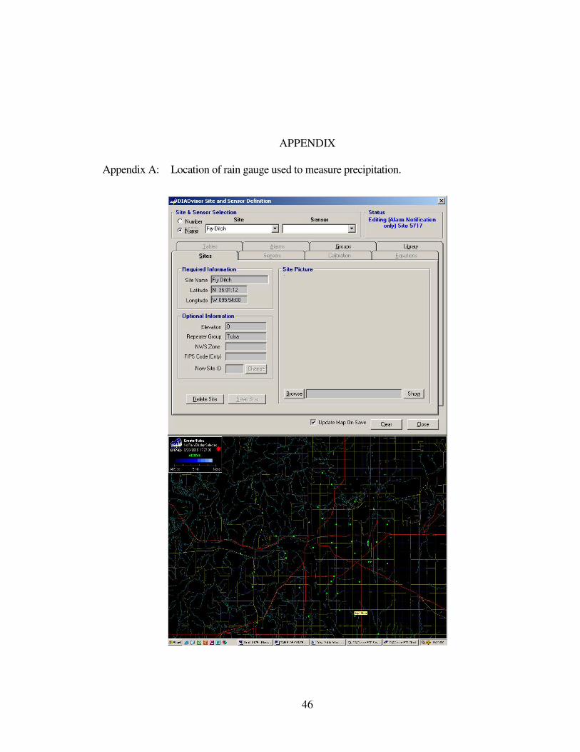
46
APPENDIX
Appendix A: Location of rain gauge used to measure precipitation.
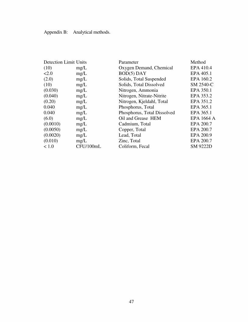
47
Appendix B: Analytical methods.
Detection Limit Units Parameter Method(10) mg/L Oxygen Demand, Chemical EPA 410.4<2.0 mg/L BOD(5) DAY EPA 405.1(2.0) mg/L Solids, Total Suspended EPA 160.2(10) mg/L Solids, Total Dissolved SM 2540-C (0.030) mg/L Nitrogen, Ammonia EPA 350.1(0.040) mg/L Nitrogen, Nitrate-Nitrite EPA 353.2(0.20) mg/L Nitrogen, Kjeldahl, Total EPA 351.20.040 mg/L Phosphorus, Total EPA 365.10.040 mg/L Phosphorus, Total Dissolved EPA 365.1(6.0) mg/L Oil and Grease HEM EPA 1664 A(0.0010) mg/L Cadmium, Total EPA 200.7(0.0050) mg/L Copper, Total EPA 200.7(0.0020) mg/L Lead, Total EPA 200.9(0.010) mg/L Zinc, Total EPA 200.7< 1.0 CFU/100mL Coliform, Fecal SM 9222D
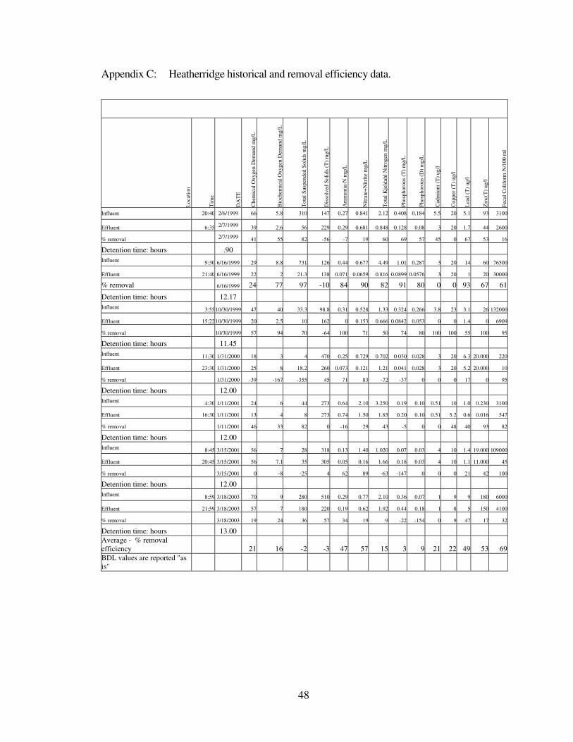
48
Appendix C: Heatherridge historical and removal efficiency data.
Loc
atio
n
Tim
e
DA
TE
Che
mic
al O
xyge
n D
eman
d m
g/L
Bio
chem
ical
Oxy
gen
Dem
and
mg/
L
Tot
al S
uspe
nded
Sol
ids
mg/
L
Dis
solv
ed S
olid
s (T
) m
g/L
Am
mon
ia-N
mg/
L
Nit
rate
+N
itri
te m
g/L
Tot
al K
jeld
ahl N
itrog
en m
g/L
Pho
spho
rous
(T
) m
g/L
Pho
spho
rous
(D
) m
g/L
Cad
miu
m (
T)
ug/l
Cop
per
(T)
ug/l
Lea
d (T
) ug
/l
Zin
c(T
) ug
/l
Fec
al C
olif
orm
N/1
00 m
l
Influent 20:40 2/6/1999 66 5.8 310 147 0.27 0.841 2.12 0.408 0.184 5.5 20 5.1 93 3100
Effluent 6:35 2/7/1999 39 2.6 56 229 0.29 0.681 0.848 0.128 0.08 3 20 1.7 44 2600
% removal 2/7/1999 41 55 82 -56 -7 19 60 69 57 45 0 67 53 16
Detention time: hours .90Influent 9:30 6/16/1999 29 8.8 731 126 0.44 0.677 4.49 1.01 0.287 3 20 14 60 76500
Effluent 21:40 6/16/1999 22 2 21.3 138 0.071 0.0659 0.816 0.0899 0.0576 3 20 1 20 30000
% removal 6/16/1999 24 77 97 -10 84 90 82 91 80 0 0 93 67 61
Detention time: hours 12.17Influent 3:5510/30/1999 47 40 33.3 98.8 0.31 0.528 1.33 0.324 0.266 3.8 23 3.1 26 132000
Effluent 15:2210/30/1999 20 2.5 10 162 0 0.153 0.666 0.0842 0.053 0 0 1.4 0 6909
% removal 10/30/1999 57 94 70 -64 100 71 50 74 80 100 100 55 100 95
Detention time: hours 11.45Influent 11:30 1/31/2000 18 3 4 470 0.25 0.729 0.702 0.030 0.028 3 20 6.3 20.000 220
Effluent 23:30 1/31/2000 25 8 18.2 260 0.073 0.121 1.21 0.041 0.028 3 20 5.2 20.000 10
% removal 1/31/2000 -39 -167 -355 45 71 83 -72 -37 0 0 0 17 0 95
Detention time: hours 12.00Influent 4:30 1/11/2001 24 6 44 273 0.64 2.10 3.250 0.19 0.10 0.51 10 1.0 0.230 3100
Effluent 16:30 1/11/2001 13 4 8 273 0.74 1.50 1.85 0.20 0.10 0.51 5.2 0.6 0.016 547
% removal 1/11/2001 46 33 82 0 -16 29 43 -5 0 0 48 40 93 82
Detention time: hours 12.00Influent 8:45 3/15/2001 56 7 28 318 0.13 1.40 1.020 0.07 0.03 4 10 1.4 19.000 109000
Effluent 20:45 3/15/2001 56 7.1 35 305 0.05 0.16 1.66 0.18 0.03 4 10 1.1 11.000 45
% removal 3/15/2001 0 -8 -25 4 62 89 -63 -147 0 0 0 21 42 100
Detention time: hours 12.00Influent 8:59 3/18/2003 70 9 280 510 0.29 0.77 2.10 0.36 0.07 1 9 9 180 6000
Effluent 21:59 3/18/2003 57 7 180 220 0.19 0.62 1.92 0.44 0.18 1 8 5 150 4100
% removal 3/18/2003 19 24 36 57 34 19 9 -22 -154 0 9 47 17 32
Detention time: hours 13.00Average - % removal efficiency 21 16 -2 -3 47 57 15 3 9 21 22 49 53 69BDL values are reported "as is"
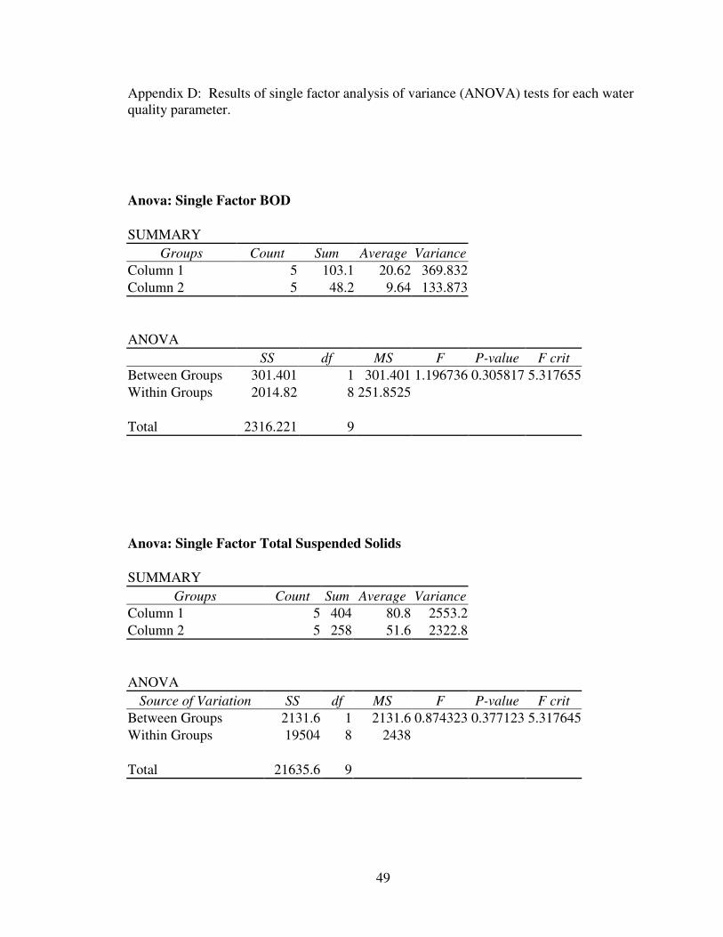
49
Appendix D: Results of single factor analysis of variance (ANOVA) tests for each water quality parameter.
Anova: Single Factor BOD
SUMMARYGroups Count Sum Average Variance
Column 1 5 103.1 20.62 369.832Column 2 5 48.2 9.64 133.873
ANOVASS df MS F P-value F crit
Between Groups 301.401 1 301.401 1.196736 0.305817 5.317655Within Groups 2014.82 8 251.8525
Total 2316.221 9
Anova: Single Factor Total Suspended Solids
SUMMARYGroups Count Sum Average Variance
Column 1 5 404 80.8 2553.2Column 2 5 258 51.6 2322.8
ANOVASource of Variation SS df MS F P-value F crit
Between Groups 2131.6 1 2131.6 0.874323 0.377123 5.317645Within Groups 19504 8 2438
Total 21635.6 9

50
Anova: Single Factor Dissolved Solids
SUMMARYGroups Count Sum Average Variance
Column 1 5 1270 254 17580Column 2 5 1110 222 370
ANOVASource of Variation SS df MS F P-value F crit
Between Groups 2560 1 2560 0.285237 0.607806 5.317645Within Groups 71800 8 8975
Total 74360 9
Anova: Single Factor Ammonia
SUMMARYGroups Count Sum Average Variance
Column 1 5 1.676 0.3352 0.128005Column 2 5 1.015 0.203 0.073095
ANOVASource of Variation SS df MS F P-value F crit
Between Groups 0.043692 1 0.043692 0.434531 0.528288 5.317645Within Groups 0.804401 8 0.10055
Total 0.848093 9

51
Anova: Single Factor Nitrate+Nitrite
SUMMARYGroups Count Sum Average Variance
Column 1 5 3.72 0.744 0.06783Column 2 5 0.814 0.1628 0.042979
ANOVASource of Variation SS df MS F P-value F crit
Between Groups 0.844484 1 0.844484 15.24212 0.004518 5.317645Within Groups 0.443237 8 0.055405
Total 1.28772 9
Anova: Single Factor Total Kjeldahl Nitrogen
SUMMARYGroups Count Sum Average Variance
Column 1 5 11.58 2.316 2.95228Column 2 5 5.03 1.006 0.13618
ANOVASource of Variation SS df MS F P-value F crit
Between Groups 4.29025 1 4.29025 2.778245 0.134112 5.317645Within Groups 12.35384 8 1.54423
Total 16.64409 9
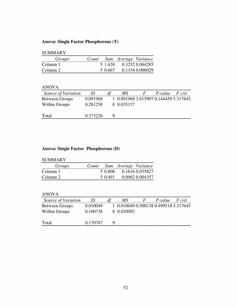
52
Anova: Single Factor Phosphorous (T)
SUMMARYGroups Count Sum Average Variance
Column 1 5 1.626 0.3252 0.064285Column 2 5 0.667 0.1334 0.006029
ANOVASource of Variation SS df MS F P-value F crit
Between Groups 0.091968 1 0.091968 2.615907 0.144459 5.317645Within Groups 0.281258 8 0.035157
Total 0.373226 9
Anova: Single Factor Phosphorous (D)
SUMMARYGroups Count Sum Average Variance
Column 1 5 0.808 0.1616 0.035827Column 2 5 0.491 0.0982 0.004357
ANOVASource of Variation SS df MS F P-value F crit
Between Groups 0.010049 1 0.010049 0.500138 0.499518 5.317645Within Groups 0.160738 8 0.020092
Total 0.170787 9

53
Anova: Single Factor Cadmium (T)
SUMMARYGroups Count Sum Average Variance
Column 1 5 0.0062 0.00124 9.3E-08Column 2 5 0.0054 0.00108 1.7E-08
ANOVASource of Variation SS df MS F P-value F crit
Between Groups 6.4E-08 1 6.4E-08 1.163636 0.31216 5.317645Within Groups 4.4E-07 8 5.5E-08
Total 5.04E-07 9
Anova: Single Factor Copper (T)
SUMMARYGroups Count Sum Average Variance
Column 1 5 0.0419 0.00838 3.85E-05Column 2 5 0.077 0.0154 0.000275
ANOVASource of Variation SS df MS F P-value F crit
Between Groups 0.000123 1 0.000123 0.786543 0.401022 5.317645Within Groups 0.001253 8 0.000157
Total 0.001376 9

54
Anova: Single Factor Lead (T)
SUMMARYGroups Count Sum Average Variance
Column 1 5 0.019 0.0038 3.06E-06Column 2 5 0.01 0.002 0
ANOVASource of Variation SS df MS F P-value F crit
Between Groups 8.1E-06 1 8.1E-06 5.294118 0.0504 5.317645Within Groups 1.22E-05 8 1.53E-06
Total 2.03E-05 9
Anova: Single Factor Zinc (T)
SUMMARYGroups Count Sum Average Variance
Column 1 5 0.207 0.0414 0.00042Column 2 5 0.072 0.0144 5.43E-05
ANOVASource of Variation SS df MS F P-value F crit
Between Groups 0.001823 1 0.001823 7.680152 0.024248 5.317645Within Groups 0.001898 8 0.000237
Total 0.003721 9
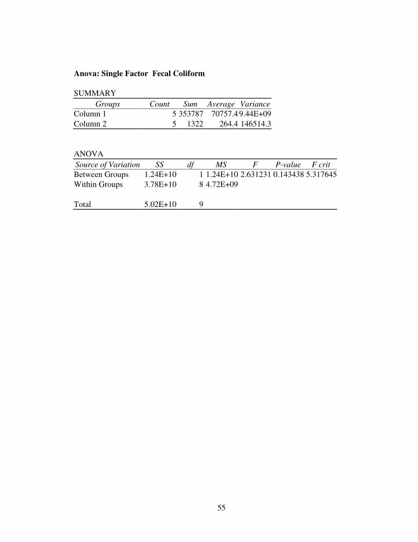
55
Anova: Single Factor Fecal Coliform
SUMMARYGroups Count Sum Average Variance
Column 1 5 353787 70757.4 9.44E+09Column 2 5 1322 264.4 146514.3
ANOVASource of Variation SS df MS F P-value F critBetween Groups 1.24E+10 1 1.24E+10 2.631231 0.143438 5.317645Within Groups 3.78E+10 8 4.72E+09
Total 5.02E+10 9

VITA
Steven Phillip Schaal
Candidate for the Degree of
Master of Science
Thesis: Water Quality Enhancement Assessment of an Existing Flood Control Detention Facility in the City Of Tulsa, Oklahoma
Major Field: Environmental Science
Biographical:
Education: Bachelor of Science in Agriculture from Southwest Texas State University, San Marcos, Texas in August 1994. Completed the requirements for the Master of Science degree with a major in Environmental Science at Oklahoma State University in July, 2006.
Name: Steve Schaal Date of Degree: July, 2006
Institution: Oklahoma State University Location: Tulsa, Oklahoma
Title of Study: WATER QUALITY ENHANCEMENT ASSESSMENT OF AN EXISTING FLOOD CONTROL DETENTION FACILITY IN THE CITY OF TULSA, OKLAHOMA
Pages in Study: 55 Candidate for the Degree of Master of Science
Major Field: Environmental Science
Scope and Method of Study: Stormwater utility managers use constructed wetlands to mediate
flooding and enhance water quality in urban watersheds. The National Pollution
Discharge Elimination System requires permit holders to assess the feasibility of
retrofitting existing flood control devices to provide additional pollutant removal from
stormwater. Chemical measurements from five storm event flows were taken of the
influent and effluent of a constructed wetland in the spring of 2005, to quantify any
change in water quality attributed to this multiple-use stormwater management facility.
Results of the study demonstrate removal of 12 of the 14 stormwater contaminants. A
dye tracer was used as a tool to ensure the same parcel of water was sampled at both the
influent and effluent.
Findings and Conclusions: The average percent difference of means ranged from 99% to a
negative 66% for fecal coliform and copper respectively. The percent difference of means
for nitrate and nitrite nitrogen was 60% and the values were significantly lower at the
outflow as compared to the inflow (p=0.004). The relative fluorescence of dye at the
effluent was used as to tool in quantifying the detention time for individual events.
ADVISER’S APPROVAL: William W. Clarkson