Embed Size (px)
Citation preview

Water Quality Models for Supporting
Shellfish Harvesting Area Management
by
Andrew David Gronewold
Department of Environmental Sciences and PolicyDuke University
Date:Approved:
Dr. Kenneth Reckhow, co-supervisor
Dr. Robert Wolpert, co-supervisor
Dr. Rachel Noble
Dr. William Kirby-Smith
Dissertation submitted in partial fulfillment of therequirements for the degree of Doctor of Philosophy
in the Department of Environmental Sciences and Policyin the Graduate School of
Duke University
2009

ABSTRACT
Water Quality Models for Supporting
Shellfish Harvesting Area Management
by
Andrew David Gronewold
Department of Environmental Sciences and PolicyDuke University
Date:Approved:
Dr. Kenneth Reckhow, co-supervisor
Dr. Robert Wolpert, co-supervisor
Dr. Rachel Noble
Dr. William Kirby-Smith
An abstract of a dissertation submitted in partial fulfillment of therequirements for the degree of Doctor of Philosophy
in the Department of Environmental Sciences and Policyin the Graduate School of
Duke University
2009

Copyright c© 2009 by Andrew David Gronewold
All rights reserved

Abstract
This doctoral dissertation presents the derivation and application of a series of wa-
ter quality models and modeling strategies which provide critical guidance to wa-
ter quality-based management decisions. Each model focuses on identifying and
explicitly acknowledging uncertainty and variability in terrestrial and aquatic envi-
ronments, and in water quality sampling and analysis procedures. While the mod-
eling tools I have developed can be used to assist management decisions in waters
with a wide range of designated uses, my research focuses on developing tools which
can be integrated into a probabilistic or Bayesian network model supporting total
maximum daily load (TMDL) assessments of impaired shellfish harvesting waters.
Notable products of my research include a novel approach to assessing fecal indica-
tor bacteria (FIB)-based water quality standards for impaired resource waters and
new standards based on distributional parameters of the in situ FIB concentration
probability distribution (as opposed to the current approach of using most probable
number (MPN) or colony-forming unit (CFU) values). In addition, I develop a model
explicitly acknowledging the probabilistic basis for calculating MPN and CFU values
to determine whether a change in North Carolina Department of Environment and
Natural Resources Shellfish Sanitation Section (NCDENR-SSS) standard operating
procedure from a multiple tube fermentation (MTF)-based procedure to a membrane
filtration (MF) procedure might cause a change in the observed frequency of water
quality standard violations. This comparison is based on an innovative theoretical
model of the MPN probability distribution for any observed CFU estimate from the
same water quality sample, and is applied to recent water quality samples collected
and analyzed by NCDENR-SSS for fecal coliform concentration using both MTF
and MF analysis tests. I also develop the graphical model structure for a Bayesian
iv

network model relating FIB fate and transport processes with water quality-based
management decisions, and encode a simplified version of the model in commercially
available Bayesian network software. Finally, I present a Bayesian strategy for cali-
brating bacterial water quality models which improves model performance by explic-
itly acknowledging the probabilistic relationship between in situ FIB concentrations
and common concentration estimating procedures.
v

Contents
Abstract iv
List of Figures ix
List of Tables xiii
Acknowledgments xiv
1 Introduction 1
1.1 Dissertation Organization . . . . . . . . . . . . . . . . . . . . . . . . 4
2 Developing a Graphical Model 8
2.1 Selecting the Model Endpoint . . . . . . . . . . . . . . . . . . . . . . 9
2.2 Terrestrial Fate and Transport . . . . . . . . . . . . . . . . . . . . . . 12
2.3 Aquatic Fate and Transport . . . . . . . . . . . . . . . . . . . . . . . 17
2.3.1 Bacteria loss models . . . . . . . . . . . . . . . . . . . . . . . 18
2.3.2 Bacteria transport models . . . . . . . . . . . . . . . . . . . . 23
2.4 Summary . . . . . . . . . . . . . . . . . . . . . . . . . . . . . . . . . 28
3 Developing and Applying a Simple Bayesian Network Model 30
3.1 Background . . . . . . . . . . . . . . . . . . . . . . . . . . . . . . . . 31
3.2 Bayesian Networks . . . . . . . . . . . . . . . . . . . . . . . . . . . . 33
3.3 Methods . . . . . . . . . . . . . . . . . . . . . . . . . . . . . . . . . . 36
3.3.1 Study Area and Data Collection . . . . . . . . . . . . . . . . . 36
3.3.2 Model Variables . . . . . . . . . . . . . . . . . . . . . . . . . . 38
3.3.3 Conditional Probabilities . . . . . . . . . . . . . . . . . . . . . 41
3.4 Results and Discussion . . . . . . . . . . . . . . . . . . . . . . . . . . 45
vi

3.5 Conclusions . . . . . . . . . . . . . . . . . . . . . . . . . . . . . . . . 48
4 An Assessment of Fecal Indicator Bacteria-Based Water QualityStandards and Water Quality Model Endpoints 50
5 Modeling the Relationship Between Most Probable Number (MPN)and Colony Forming Unit (CFU) Estimates of Fecal IndicatorBacteria Concentrations 60
5.1 Introduction . . . . . . . . . . . . . . . . . . . . . . . . . . . . . . . . 61
5.2 Methods . . . . . . . . . . . . . . . . . . . . . . . . . . . . . . . . . . 66
5.2.1 Water Quality Monitoring . . . . . . . . . . . . . . . . . . . . 66
5.2.2 Theoretical Probability Model . . . . . . . . . . . . . . . . . . 67
5.2.3 OLS Regression Empirical model . . . . . . . . . . . . . . . . 67
5.3 Results and Discussion . . . . . . . . . . . . . . . . . . . . . . . . . . 68
5.4 Conclusions . . . . . . . . . . . . . . . . . . . . . . . . . . . . . . . . 71
5.5 Calculations . . . . . . . . . . . . . . . . . . . . . . . . . . . . . . . . 72
6 Improving Parameter Estimation in the Aquatic Fate and Trans-port Model 79
6.1 Introduction . . . . . . . . . . . . . . . . . . . . . . . . . . . . . . . . 80
6.1.1 Serial Dilution Analysis . . . . . . . . . . . . . . . . . . . . . 81
6.1.2 Most Probable Number Calculations . . . . . . . . . . . . . . 82
6.2 Methods . . . . . . . . . . . . . . . . . . . . . . . . . . . . . . . . . . 85
6.2.1 Data Simulation . . . . . . . . . . . . . . . . . . . . . . . . . . 86
6.2.2 Parameter Estimation . . . . . . . . . . . . . . . . . . . . . . 91
6.3 Results . . . . . . . . . . . . . . . . . . . . . . . . . . . . . . . . . . . 92
6.4 Discussion . . . . . . . . . . . . . . . . . . . . . . . . . . . . . . . . . 93
6.5 Conclusions . . . . . . . . . . . . . . . . . . . . . . . . . . . . . . . . 99
vii

6.6 Computer code . . . . . . . . . . . . . . . . . . . . . . . . . . . . . . 101
A Listing of Impaired Waters 103
B North Carolina Shellfish Harvesting Area Water Quality Standards104
Bibliography 106
Biography 117
viii

List of Figures
2.1 Graphical representation of critical environmental system responsevariables and potential model endpoints. Management decisions areindicated by boxes, and variables are represented by rounded nodes. . 11
2.2 Graphical representation of assumed system variables and causal rela-tionships for terrestrial fate and transport of fecal indicator bacteria.Management decisions are indicated by boxes, and variables are rep-resented by rounded nodes. . . . . . . . . . . . . . . . . . . . . . . . . 17
2.3 Graphical representation of environmental processes and system vari-ables affecting aquatic fate and transport of fecal indicator organisms.Management decisions are indicated by boxes, and variables are rep-resented by rounded nodes. . . . . . . . . . . . . . . . . . . . . . . . . 28
2.4 Comprehensive graphical network of fecal contamination in designatedresource waters. Management decisions are indicated by boxes, andvariables are represented by rounded nodes. . . . . . . . . . . . . . . 29
3.1 Simple network model representing rainfall-induced fecal contamina-tion of a coastal estuary. . . . . . . . . . . . . . . . . . . . . . . . . . 34
3.2 Graphical representation of Bayes’ theorem indicating prior and pos-terior probability densities, and the normalized likelihood for a waterquality standard. . . . . . . . . . . . . . . . . . . . . . . . . . . . . . 36
3.3 Graphical representation of environmental variables and processes as-sociated with fecal contamination in tidal shellfish harvesting areas.Management decisions are indicated by boxes, and variables are rep-resented by rounded nodes. . . . . . . . . . . . . . . . . . . . . . . . . 39
3.4 Graphical submodel relating precipitation events, tidal dynamics, andwater quality. Probabilities for all variable states are based on moni-toring data collected between 1994 and 1997 at a cluster of monitoringstations in the upper reaches of the Newport River Estuary, NorthCarolina. . . . . . . . . . . . . . . . . . . . . . . . . . . . . . . . . . . 41
ix

3.5 Conditional probability distribution table for fecal coliform MPN node.For each of the three states of the MPN node, each row indicates themarginal probability of the node being in that state given the state ofthe three causal variables. For example, the probability that the MPNis less than 14 organisms per 100 ml, given that the tide is rising, themost recent rainfall was less than one inch, and that it has been lessthan four days since the most recent rain event, is 0.667. . . . . . . . 44
3.6 Graphical submodel relating precipitation events, tidal dynamics, andwater quality. Probabilities for fecal coliform MPN states are condi-tional upon long-term average precipitation and tidal conditions in theupper reaches of the Newport River Estuary, North Carolina. . . . . . 45
4.1 Prior and posterior distributions for σk for five randomly selected sta-tions in the Newport River using the three priors in table 4.4. Eachrow utilizes the same prior distribution, and each column represents aseparate station. Vertical gray lines are added to facilitate comparisonbetween alternative priors for each station. . . . . . . . . . . . . . . . 53
4.2 Combinations of the mean µc and standard deviation σc of the log-transformed fecal coliform concentration distribution which yieldedMPN (solid lines) or CFU (dashed lines) samples in violation of theNSSP median standard (panel a), geometric mean standard (panel b),90th percentile standard (panel c), or any standard (panel d) with afrequency of either 0.005 or 0.1. The zone of violations is in the upperright of each panel. . . . . . . . . . . . . . . . . . . . . . . . . . . . . 54
4.3 Relationship between the mean µc and standard deviation σc of the log-transformed fecal coliform concentration distribution and simulatedviolation of any CFU-based water quality standard (dashed lines) andany MPN-based water quality standard (solid lines) for possible val-ues of the negative binomial dispersion parameter α. Panels a and bindicate µc − σc pairs expected to violate standards with a frequencyof 0.1 and 0.005, respectively. . . . . . . . . . . . . . . . . . . . . . . 55
4.4 Log-likelihood (solid line) of transformation parameter γ for σc usingpaired values of µc and σc. Panel a based on values from table 4.2 forσc > 0.65, panel b based on values from table 4.2 for σc ≤ 0.65, panelc based on values from table 4.3 for σc > 0.65, and panel d based onvalues from table 4.3 for σc ≤ 0.65. . . . . . . . . . . . . . . . . . . . 56
x

4.5 Violation contour lines overlaid by violation line best-fit regressionmodel fitted values based on model parameters in table 4.5. . . . . . . 57
4.6 Joint posterior probability density contour lines (solid lines) for fourmonitoring stations in the Newport River Estuary. Dashed lines in-dicate combinations of the mean µc and standard deviation σc of thelog-transformed fecal coliform concentration distribution which violateconcentration-based standards no more than 0.5% of the time usingMPN or CFU standards as the reference. Confidences of compliance(CC) are given in the lower left of each panel for both MPN and CFU-based standards. . . . . . . . . . . . . . . . . . . . . . . . . . . . . . 59
5.1 Expected values and 95% prediction sets or prediction intervals forobservable fecal coliform MPN (panel A) and CFU (panel B) measure-ments given the true fecal coliform concentration in organisms per 100ml. For clarity, expected values and 95% prediction sets or intervalsare plotted only for every 5th integer-valued concentration c. Maxi-mum true concentrations in each plot are based on maximum MPNand CFU observations in the NCDENR-SSS data set. CFU predictionintervals are based on an MF sample aliquot volume of 100 ml. . . . . 75
5.2 Expected value and 95% credible intervals for the fecal coliform trueconcentration given MPN (panel A) and CFU (panel B) estimates inorganisms per 100 ml. For clarity, panel A includes only the 51 observ-able MPN estimates presented in standard laboratory analysis MTFconversion tables for the 5-tube serial dilution analysis procedure (see,e.g. Woodward, 1957) and panel B includes only every 5th observableCFU value based on an MF test with a sample aliquot volume of 100ml. . . . . . . . . . . . . . . . . . . . . . . . . . . . . . . . . . . . . . 76
5.3 Empirical linear regression model (panel A) and theoretical probabilitymodel (panel B) of the relationship between fecal coliform MPN andCFU estimates from the same water quality sample. . . . . . . . . . . 77
5.4 Observed values, expected values, and the theoretical probability massfunction of the MPN for a CFU measurement from the same waterquality sample. Observed values are from recent NCDENR-SSS study. 78
xi

6.1 Estimated inner quartile (50%, thick black line) and 95% intervals(thin black line) for each model parameter based on samples of size10, 25, or 100. Vertical gray lines indicate the parameter value usedto simulate data. Dots (solid and hollow) indicate median values.For each sample size, the upper line (with solid circle) represents theparameter estimate based on using the MPN point estimate, and thelower line (with hollow circle) represents parameter estimates basedon using the pattern of positive tubes for model calibration. . . . . . 93
6.2 Estimated inner quartile (50%, thick black line) and 95% intervals(thin black line) for model-predicted FIB concentrations at time t =1, 4, and 7 days. Vertical gray lines indicate the expected FIB con-centration using the “true” parameter values. Dots (solid and hollow)indicate median values. For each sample size, the upper line (withsolid circle) represents predicted FIB concentrations using the modelcalibrated with MPN point estimates, and the lower line (with hol-low circle) represents predicted FIB concentrations using the modelcalibrated using the pattern of positive tubes. . . . . . . . . . . . . . 95
xii

List of Tables
3.1 Marginal distribution of fecal coliform MPN results at a selected group-ing of monitoring stations. Newport River, North Carolina. . . . . . . 46
3.2 Summary of Bayesian analysis results for Newport River, North Car-olina fecal coliform MPN data. . . . . . . . . . . . . . . . . . . . . . . 47
4.1 NSSP shellfish harvesting area fecal coliform water quality standardsbased on a minimum of 30 randomly collected samples. . . . . . . . . 51
4.2 Values of µc and σc constituting MPN contour line (for simulated vi-olation frequency = 0.005). . . . . . . . . . . . . . . . . . . . . . . . 51
4.3 Values of µc and σc constituting CFU contour line (for simulated vio-lation frequency = 0.005). . . . . . . . . . . . . . . . . . . . . . . . . 52
4.4 Alternative priors for true concentration ck standard deviation σk atstation k. . . . . . . . . . . . . . . . . . . . . . . . . . . . . . . . . . 52
4.5 Regression model parameters including transformation parameter (γ),intercept (β0), and slope (β1). . . . . . . . . . . . . . . . . . . . . . . 52
4.6 Estimated confidence of compliance (CC), posterior probability of vi-olating any MPN standard, and observed violations for monitoringstations in the Newport River Estuary during the 2000-2005 assess-ment period. . . . . . . . . . . . . . . . . . . . . . . . . . . . . . . . . 58
6.1 Example of simulated data set with sample size j = 10. Each rowrepresents a simulated grab sample with concentration c collected attime t, a simulated pattern of positive tubes (x1, x2, x3) resulting fromstandard MTF decimal dilution analysis of the grab sample, and thecorresponding MPN (**see Methods section for interpretation of re-sults with all tubes negative, or all tubes positive). . . . . . . . . . . 89
6.2 Simulation steps . . . . . . . . . . . . . . . . . . . . . . . . . . . . . . 90
A.1 Water bodies within shellfish growing area E-4 and their status relativeto the 303(d) list of impaired waters. “IR Category” refers to 2008Draft Integrated Report (IR) Category. . . . . . . . . . . . . . . . . . 103
xiii

Acknowledgments
I would like to thank the members of my doctorate committee, particularly Dr. Ken
Reckhow for agreeing to take me on as a graduate student, and for providing me not
only with the opportunity to work on a focused research project closely linked to
my own interests, but also with the opportunity to explore new research trajectories.
I’m also very grateful to Dr. Robert Wolpert for agreeing to work closely on many of
the detailed statistical aspects of my research. Finally, many thanks to Dr. Rachel
Noble and Dr. Bill Kirby-Smith for your support and friendship, it has been a
pleasure working with you.
Much of the research presented in this dissertation was supported with funds
from the United States Environmental Protection Agency (USEPA) through the
North Carolina Division of Water Quality (NCDWQ) 319 program (Contract No.
EW05049). Additional funding was also provided through grants from the National
Science Foundation (NSF Grant Nos. DMS-0112069 and DMS-0422400) and (through
collaboration with Dr. Mark E. Borsuk) the EPA Office of Research and Develop-
ment’s Advanced Monitoring Initiative (AMI) Pilot Projects Focused on GEOSS
(Global Earth Observation System of Systems). I am also very grateful for scholar-
ship support from the Water Environment Federation (WEF), Quantitative Environ-
mental Analysis (QEA), LLC, and the North Carolina Association of Environmental
Professionals (NCAEP).
I owe tremendous thanks to the staff at NCDENR-SSS, including Patti Fowler,
xiv

J.D. Potts, Andrew Haines, Shannon Jenkins, Nadine Stoddard, and Diane Mason,
all of whom were consistently generous with their time in answering questions, sharing
and explaining water quality analysis data, and teaching me about their analytical
procedures. Most, if not all, of this dissertation would not have been possible without
their help. I also owe thanks to Larry Wood and his family not only for their kindness
over the years, but also for teaching me about sailing, shellfishing, and appreciating
the beauty and joy found in natural resources, particularly those of Waquoit Bay on
Cape Cod.
Several colleagues from the Nicholas School, particularly those who are either
current or former members of Ken Reckhow’s laboratory group, provided critical
feedback at various stages of my research. In particular, thanks go to Ben Best, Joe
Sexton, Craig Stow, Song Qian, Sean McMahon, Scott Loarie, Rob Schick, Ibrahim
Alameddine, Lori Bennear, Richard Anderson, and Conrad Lamon. I also owe thanks
to my former colleagues at Stearns & Wheler, LLC, particulary Bill Hall, Jr. and
Nate Weeks, both of whom provided kind assurance both during my graduate studies,
and in my decision to return to graduate school. Many thanks also go out to the
hard work of master’s students who contributed to research on the Newport River
including Tammy Hill, Whan Chunkrua, and Ryan O’Banion.
My family is fortunate enough to live in a wonderful community in Old West
Durham, and the support from our friends and neighbors has been invaluable, par-
ticularly from Cyrus, Michelle, Julie, Nancy, Guy, Colleen, Riley, Patrick and Ally.
xv

Jim and Meg Lister also provided invaluable support, keeping my family fed and on
the right parenting track during the first few months after Michael and John were
born. We could not have survived parenting twins, nor could I have maintained
progress in my Ph.D. program, without your help. I also appreciate the one-on-one
help from many of the staff here at the Nicholas School, including Jacqui Franklin,
Deborah Wilson, Nancy Morgans, Laura Turcotte, Stephen Cash, and Meg Stephens.
I also owe special thanks to Lana BenDavid and the graduate school for their support.
I will be indebted for a very long time (if not forever) to my family, particularly
those who managed to survive staying in our crazy home while we tried to raise
twins, support a doctoral dissertation, and do all the other things families try to do.
In particular, Peter and Marcia provided critical support during a major transition
period. Granny and Pop-pop, I hope it goes without saying that your love and
support have made all the different in the world. Mom and Dad, thank you for
everything. Most of all, thank you Sara. When I asked you to marry me, I failed
to mention that I planned on quitting my job, going back to graduate school in
North Carolina, buying a house, and immediately having twins. Thanks for keeping
everything (including yourself) afloat.
xvi

Chapter 1
Introduction
This doctoral dissertation presents the derivation and application of a series of wa-
ter quality models and modeling strategies which provide critical guidance to water
quality-based management decisions by identifying and explicitly acknowledging un-
certainty and variability in terrestrial and aquatic environments, and in water qual-
ity sampling and analysis procedures. While these modeling tools can be used to
assist management decisions in waters with a wide range of designated uses, my re-
search focuses on developing tools which can be integrated into a probabilistic or
Bayesian network model supporting total maximum daily load (TMDL) assessments
of impaired shellfish harvesting waters. Such a model is currently being developed
through an ongoing 319 project with the North Carolina Division of Water Quality,
and a major goal of this dissertation is to provide tools which will improve the per-
formance of that model. Therefore, the research presented in this dissertation should
be viewed as a component of a more comprehensive modeling and research effort.
While my research provides the foundation for building a Bayesian or probabilistic
network model, the final model is not presented explicitly as part of this dissertation.
Section 303(d) of the United States (US) Clean Water Act requires that states
assess the condition of surface waters and report those which fail to meet ambient
water quality standards (Smith et al., 2001; Houck, 2002). These are added to the
1

US Environmental Protection Agency (EPA) list of impaired waters (U.S. Environ-
mental Protection Agency, 2005b) and can only be removed after the performance
of a TMDL assessment (National Research Council, 2001; Cooter, 2004) followed by
sample-based verification that the standards are being met. As with any TMDL
assessment, the primary objective of the Newport River TMDL is to determine the
maximum allowable pollutant load from point, non-point, and natural sources, in-
cluding a margin of safety (MOS), which can be discharged into a receiving water
without violating water quality standards (National Research Council, 2001; Houck,
2002). Such predictive assessments are usually based on an empirical or mechanistic
water quality model relating pollutant loading levels to water body concentrations
(Borsuk et al., 2002; Benham et al., 2006). Fecal indicator bacteria (FIB), such
as fecal coliform, are commonly used to assess potential pathogen contamination in
coastal waters, and serve as the pollutant of concern for the models presented in this
dissertation (U.S. Environmental Protection Agency, 2001).
Model Ordinance in the Guide for the Control of Molluscan Shellfish, prepared by
the National Shellfish Sanitation Program (NSSP), includes recommended FIB-based
water quality criteria for shellfish-growing waters (Food and Drug Administration
and Interstate Shellfish Sanitation Conference, 2005). States which participate in
the NSSP, and which are also members of the Interstate Shellfish Sanitation Confer-
ence, enforce the Model Ordinance as a minimum requirement for sanitary control of
shellfish (Food and Drug Administration and Interstate Shellfish Sanitation Confer-
2

ence, 2005). Similar FIB-based water quality standards are enforced in surface waters
with other designated uses, such as recreational use (N.C. Department of Environ-
ment and Natural Resources, 2004) and drinking water supply (U.S. Environmental
Protection Agency, 2005a).
The latest official assessment of US water quality data (U.S. Environmental Pro-
tection Agency, 2002) indicates that pathogens are the leading cause of coastal shore-
line standard violations (275 total miles impaired) and the second leading cause of
violations in rivers and streams (82,100 total miles impaired). The Newport River
Estuary and its tributaries, which are collectively designated as growing area E-4
by the North Carolina Department of Environment and Natural Resources Shellfish
Sanitation and Recreational Water Quality Section (NCDENR-SSS), is historically a
productive shellfish harvesting area. However, all of its segments and tributaries are
either permanently or conditionally closed to shellfishing based on poor water qual-
ity or proximity to known or potential sources of fecal contamination. As a result,
growing area E-4 comprises forty of the designated shellfish harvesting areas in North
Carolina which are currently included in the USEPA 303(d) list and therefore require
a TMDL assessment (see appendix A). Developing modeling tools which support
TMDL assessments in this area not only addresses an acute need, but also provides
additional context for addressing pathogen water quality problems around the US
and the world.
3

1.1 Dissertation Organization
My dissertation is divided into 6 chapters. This Chapter (Chapter 1) describes the
rationale for my doctorate research including overall research objectives and critical
regulatory requirements. Chapter 2 proposes a new graphical structure for either
a probabilistic or Bayesian network model of water quality in shellfish harvesting
waters. USEPA recommends initiating TMDL projects with an evaluation of ap-
propriate water quality indicators and associated target values which can be used
to assess attainment of the designated use (U.S. Environmental Protection Agency,
2001). Therefore, while chapter 2 defines (rather broadly) the scope of any bacte-
rial TMDL assessment, it also highlights a poorly-defined relationship between water
quality model endpoints and proposed measures of water quality (including alterna-
tive indicator organisms and different testing methods) as well as potential risks to
human and environmental health. Although my dissertation focuses on mitigating
fecal contamination in shellfishing resource areas (and reducing subsequent risk of
the outbreak of shellfish-borne infectious diseases), Chapter 2 serves as a reminder
that pollutants of non-fecal origin (such as red-tide causing ciguatoxins) might be
integrated into ongoing health risk-based management planning (Hackney and Pier-
son, 1994). Chapter 2 indicates a growing need in the microbial analysis and water
quality modeling field to more explicitly quantify the relationship between human
health risks and alternative measures of fecal and non-fecal contamination in coastal
resource waters. Identifying this research need was a major result of the early stages
4
of my research, and establishes the context for all subsequent Chapters of my dis-
sertation. Much of the research presented in Chapter 2 appears in peer-reviewed
proceedings of the International Water Association (IWA) WaterMatex 2007 Confer-
ence (Gronewold and Reckhow, 2007).
In Chapter 3, I develop and apply a simplified version of the conceptual graphical
model from Chapter 2 to water quality monitoring data from the Newport River
using the Bayesian analysis software package Neticar. This analysis identifies how
presumed critical environmental variables impact water quality-based management
decisions, and whether or not those variables are monitored under truly random con-
ditions. Furthermore, the initial modeling effort in Chapter 3 indicates that critical
model variables (such as the model endpoint) should explicitly acknowledge uncer-
tainty and variability (through, for example, probabilistic models) to allow compari-
son between model output and management decision criteria. The work in Chapter
3 also suggests that fecal indicator bacteria concentration forecasting models must
appropriately reflect uncertainty inherent to specific bacteria water quality analysis
procedures, and that the Neticar software package may not be the most appropriate
tool for doing so. The research in Chapter 3 appears in peer-reviewed conference
proceedings of the Water Environment Federation TMDL 2007 Specialty Conference
held in Bellevue, Washington (Gronewold et al., 2007).
In Chapter 4, I develop a novel approach to assessing FIB-based water quality
standards for pathogenically-impaired resource waters and propose new standards
5

based on distributional parameters of the in situ FIB concentration probability dis-
tribution (as opposed to the current approach of using most probable number (MPN)
or colony-forming unit (CFU) values). This work is motivated by recommendations
of the National Research Council (2001), and an exploratory analysis of historic New-
port River water quality and environmental data, which suggest that several water
bodies in shellfish growing area E-4 either do not appear to violate water quality
standards, or do not have sufficient data to justify being included in the 303(d) list.
Chapter 4 concludes with a re-evaluation of water quality standard violations in the
Newport River based on my proposed water quality standards. Much of the work
(and text) in Chapter 4 was developed in collaboration with Dr. Mark Borsuk, Dr.
Robert Wolpert, and Dr. Kenneth Reckhow and was recently published (as the cover
article) in Environmental Science & Technology (Gronewold et al., 2008).
Chapter 5 compares different FIB water quality metrics in order to determine
whether an ongoing change in NCDENR-SSS standard operating procedure (and
elsewhere, presumably) from a multiple tube fermentation (MTF)-based procedure
to a membrane filtration (MF) procedure might cause a change in the observed fre-
quency of water quality standard violations. This comparison is based on an inno-
vative theoretical model of the MPN probability distribution for any observed CFU
estimate from the same water quality sample, and is applied to recent water quality
samples collected and analyzed by NCDENR-SSS for fecal coliform concentration us-
ing both MTF and MF analysis tests. This research provides important insight into
6

whether MPN and CFU intra-sample variability stems from human error, laboratory
procedure variability, or is simply a consequence of the probabilistic basis for calcu-
lating the MPN. This research was conducted in close collaboration with Dr. Robert
Wolpert, and was recently published in Water Research (Gronewold and Wolpert,
2008).
Finally, in Chapter 6, I propose a Bayesian strategy to calibrating FIB water
quality models in which the pattern of positive tubes from a multiple-tube fermen-
tation (MTF) serial dilution analysis is used as data. My proposed strategy assumes
that the pattern of positive tubes or wells in a serial dilution analysis experiment
(using, for example, either the MTF test or IDEXX Quanti-Trayr/2000 system),
when modeled as a series of stochastic random variables, reflects variability in serial
dilution analysis procedures and, consequently, uncertainty in the estimate of the true
FIB concentration. I then compare my proposed Bayesian strategy with the common
practice of using MPN point estimates to calibrate FIB water quality models. The
research presented in Chapter 6 highlights how proper acknowledgement (or igno-
rance) of model input uncertainty affects both FIB water quality model parameter
estimates as well as model-based management decisions. Much of this research was
completed in collaboration with Dr. Song Qian, Dr. Robert Wolpert, Dr. Rachel
Noble and Dr. Kennth Reckhow, and is currently being revised following submittal
to Water Research.
7

Chapter 2
Developing a Graphical Model
Note: much of the text from this Chapter appears in peer-reviewed proceedings of the
International Water Association (IWA) WaterMatex 2007 conference (Gronewold
and Reckhow, 2007).
Appropriate graphical representation of assumed relationships between environ-
mental system variables, resource area management actions, and human health im-
pacts is the first and potentially most critical stage in the development of a proba-
bilistic or Bayesian network model designed to protect designated resource waters.
A graphical network establishes the cornerstone on which model algorithms are iden-
tified and applied, monitoring plans are implemented, and management alternatives
are evaluated. Furthermore, a graphical model structure facilitates group model
building and dissemination of these model algorithms and assumptions about system
dynamics (Borsuk et al., 2004).
In this Chapter, I present a step-by-step approach to developing a graphical net-
work relating system variables and management actions associated with fecal con-
tamination of resource waters. This graphical network model serves as a foundation
for future implementation of a probabilistic or Bayesian network model designed
to integrate environmental conditions in bacteriologically impaired surface waters
8

with management alternatives, and to forecast probability distributions of designated
model endpoints.
2.1 Selecting the Model Endpoint
Long-term water resource management projects, such as those implemented through
the TMDL program, should start with an evaluation of appropriate water quality
indicators and associated target values which can be used to assess designated use
attainment (U.S. Environmental Protection Agency, 2001). Current guidelines for
United States shellfish harvesting waters, for example, indicate fecal coliform most
probable number (MPN) and colony forming unit (CFU) values are the basis for water
quality standards, and therefore serve as logical model endpoints (Food and Drug Ad-
ministration and Interstate Shellfish Sanitation Conference, 2005). Recent research,
however, indicates that several alternative indicator organisms may more accurately
reflect the potential health risk associated with fecal contamination (National Re-
search Council, 2001; U.S. Environmental Protection Agency, 2001). Potential alter-
native indicators of fecal contamination include the family of coliform bacteria (which
include total coliform, fecal coliform, and Escherichia coli), fecal streptococci (U.S.
Environmental Protection Agency, 2001; Kashefipour et al., 2005), and Enterococcus
sp (Sanders et al., 2005). Furthermore, while indicator organism concentrations in
the water column are the standard for assessing water quality and threats of fecal
contamination, human illness and death may also occur from the consumption of
9

shellfish contaminated with pollutants of non-fecal origin (such as red-tide causing
ciguatoxins), even if the shellfish are properly cooked. Several authors, including
Hackney and Pierson (1994), provide a history of field studies relating human disease
outbreaks with contamination of shellfishing resource areas.
Other human and environmental health measures not directly linked to TMDL
implementation, but of significant concern to public health officials and the public-
at-large, include potential relationships between fecal coliform concentration in the
water column and underlying shellfish tissue, the relationship between fecal indicator
organism concentration in shellfish tissue and risk of human illness, and the relation-
ship (in any media, including waters and shellfish tissue) between fecal indicator and
pathogenic organism concentrations. These environmental and human health vari-
ables are included in the graphical network to improve model flexibility and facilitate
future adaptation to alternative management scenarios, and applications other than
strictly TMDL support.
However, because this dissertation is primarily intended to support the TMDL
assessment process and, in particular, the development of TMDLs in shellfish har-
vesting waters, the model endpoint assumed for most of this dissertation is surface
water fecal coliform concentration assessed using currently approved analytical tech-
niques and standards. I propose this endpoint with implicit understanding that fecal
coliform (or other indicator organism) aquatic and terrestrial transport and transfor-
mation processes used to establish conditional probability relationships in the net-
10

work model are not likely to accurately represent fate and transport dynamics of the
pathogens they supposedly represent. Developing a network model structure which
can be adapted to a variety of potential model endpoints, including both pathogenic
and non-pathogenic organisms of fecal origin, is an area for additional research. My
proposed graphical representation of critical model endpoints, including critical en-
vironmental system response variables, management decisions, and potential model
endpoints is included in figure 2.1.
Figure 2.1: Graphical representation of critical environmental system response vari-ables and potential model endpoints. Management decisions are indicated by boxes,and variables are represented by rounded nodes.
Uncertainty associated with some fecal indicator organism laboratory analysis
procedures can range up to an order of magnitude, and has significant impacts on
both management actions and perceptions of threats to human health. Though not
immediately obvious in figure 2.1, network models provide a logical framework for
exposing and propagating both intrinsic sources of measurement uncertainty inherent
to bacteriological analytical procedures, as well as extrinsic sources of uncertainty,
into model endpoints. Modeling strategies for addressing these potential sources of
11

uncertainty will be addressed in detail in Chapters 4, 5, and 6.
2.2 Terrestrial Fate and Transport
In order to guide long-term management strategies, a fecal coliform pollution network
model must address the relationship between land use practices, loading reduction
measures, and predicted changes in pollutant concentration probability distribution
in the receiving water. The first relationship in this causal chain, therefore, is ter-
restrial fecal pollution deposition and wash-off. Establishing conditional probability
relationships between the variables related to this process allows loading reduction
management actions to be simulated in the model either at the pollution generation
level, or at the watershed-water body interface.
Land use practices and land cover types in the coastal watersheds of North Car-
olina, as with many other watersheds discharging into coastal shellfishing resource
waters, are dominated by agriculture and forested areas in which potential fecal
pollution sources can range from waste management infrastructure to wildlife and
agricultural runoff (Weiskel et al., 1996; White et al., 2000; Shen et al., 2005). Ter-
restrial accumulation and decay of fecal indicator bacteria from these, and similar
landscapes, can be approximated by a first-order decay process coupled with a lin-
ear daily loading rate term (Alley and Smith, 1981; U.S. Environmental Protection
Agency, 2001):
dL
dt= N(s) − kt(s)L(t) (2.1)
12

where
L(t) = number of organisms on the landscape at time t (often in days)
N(s) = seasonal terrestrial FIB deposition rate (organisms per day)
kt(s) = seasonal first-order terrestrial decay rate (1/day)
Transport of fecal pollution (following deposition on the landscape) and entrapped
indicator organisms is a complicated combination of both surface and groundwater
processes. Groundwater is a potential transport mechanism for pathogens and indi-
cator organisms if it serves as a connection between a receiving surface water and a
land-based pollution source such as a waste lagoon, leaking septic tank, or improperly
designed landfill (Ferguson et al., 2003). Soils may act as a filtering mechanism for
certain pathogens, and studies have indicated that they serve as a significant barrier
for viruses, bacteria, and protozoa (Schijven and Hassanizadeh, 2000, 2002). Trans-
port of pathogens and indicator bacteria, however, varies in any media depending
on chemical, physical, and biological properties of the media (Ferguson et al., 2003).
For example, conditions which promote transfer of pollutants to groundwater include
sudden redistribution of a pollutant-bearing liquid on the land surface (such as la-
goon waste) and naturally occurring soil macropores (e.g. root channels and animal
burrows) which limits soil attenuation (Thomas and Phillips, 1979; McMurry et al.,
1998). In general, microbial subsurface transport is poorly understood and is an
area for further research. In light of these various processes, bacteria and pathogen
terrestrial transport models often express pollutant washoff primarily as a function
of precipitation in the following form (Alley and Smith, 1981; Barbe et al., 1996):
13

dL
dt= −αrbL(t) (2.2)
where
r = precipitation intensity or effective runoff rate (inches/day)
α = washoff coefficient, with conversion units
b = power constant
Equation 2.2 is often applied using watershed-averaged values for impervious sur-
face runoff, but can be applied to pervious watersheds in which the rainfall-induced
washoff is typically less than in impervious areas. Parameter values fitted to actual
data for this model are presented in Alley and Smith (1981).
Another potential algorithm for relating pollutant loading to rainfall is (Reeves
et al., 2004):
L ∼ Qn (2.3)
where
L = pollutant load (organisms/day)
Q = volumetric flow rate (ft3/day)
n = power constant (often between 1 and 1.5)
A similar representation of this equation is the power law of the form (Lee and
Bang, 2000):
14

L
As∝
[
Q
As
]n
(2.4)
where
As = watershed area
n = power constant
Equation 2.4 can be rewritten as a linear model of the form:
ln(L
As) = ln(α) × n ln(
Q
As) (2.5)
Many of these algorithms are encompassed in water quality modeling software
packages, some of which are supported by USEPA (U.S. Environmental Protection
Agency, 2001). Ferguson et al. (2003) and Shen et al. (2005) provide comprehensive
summaries of available software packages, including:
• Hydrologic simulation program - Fortran (HSPF)
• Loading simulation program C++
• Watershed analysis risk management framework (WARMF)
• Soil and water assessment tool (SWAT)
• Agricultural nonpoint sources model
• Storm water management model (SWMM)
15

The wide range of factors and high degrees of uncertainty affecting the relation-
ship between pollutant accumulation, and washoff during precipitation events, make
collection of appropriate data for such models an often overwhelming task (National
Research Council, 2001). For example, soil moisture conditions are often considered
a critical variable in watershed runoff processes (Beven, 2001), yet the high spatial
and temporal monitoring resolution required to accurately reflect these conditions
would exhaust the resources of most management groups (National Research Coun-
cil, 2001). As a result, I have combined historic algorithms (represented by equations
2.1 and 2.2) into the following:
dL
dt= N(s) − kt(s)L(t) − αrbL(t) (2.6)
This approach has the advantage of minimizing dependency on more detailed,
small-scale terrestrial processes, many of which are poorly understood and relatively
underrepresented in the literature, including (Ferguson et al., 2003):
• transport particle size distribution
• relationship between physical properties of watersheds, microbial cellular-scale
properties, and transport phenomenon
• microbial die-off and decay upon initial transfer into aquatic environment
A graphical representation of the proposed terrestrial fate and transport compo-
nent is presented in figure 2.2.
16

Figure 2.2: Graphical representation of assumed system variables and causal rela-tionships for terrestrial fate and transport of fecal indicator bacteria. Managementdecisions are indicated by boxes, and variables are represented by rounded nodes.
2.3 Aquatic Fate and Transport
Small coastal embayments, including many tributaries of the Newport River Estuary,
are defined as partially enclosed water bodies with a connection to a larger bay or
estuary. Depths in these small coastal embayments can range between 0.5 and 3.0
meters (Fischer, 1979; Thomann and Mueller, 1987), and pollutant concentrations are
heavily influenced by tidal flushing and surface runoff. Advection and other trans-
port processes in coastal resource waters are frequently dominated by tidal activity
(Grant et al., 2001; Kashefipour et al., 2005; Sanders et al., 2005). The relatively
shallow depth and strong advective forces in small coastal embayments often result
in complete or near-complete vertical mixing (Thomann and Mueller, 1987).
17

In addition to advective forces, governing processes affecting fecal indicator organ-
ism aquatic fate and transport include settling (Chapra, 1997) and natural mortality
(Gameson and Gould, 1974; Auer and Niehaus, 1993). Mortality of biological or-
ganisms is often represented in water quality models by a first-order loss rate ka
(in units day−1), which includes effects of temperature, salinity, and solar radiation
(Chapra, 1997). In addition, coastal embayments are often surrounded by wetlands
which undergo continuous wetting and drying cycles and, as a result, may represent
a non-point source of pollution (Sanders et al., 2005).
In an effort to develop a simple and robust network model structure, I review in
detail (in the following sections) potential approaches to modeling FIB transport and
decay processes. I then extract key model algorithms to be represented in the final
network model.
2.3.1 Bacteria loss models
Bacteria die-off and decay in aquatic environments is typically represented in water
quality models by an effective loss rate, ka (in units day−1) accounting for natural
mortality, solar radiation, and settling (Chapra, 1997):
ka = kad+ kai
+ kas (2.7)
where kadrepresents natural mortality, kai
represents mortality due to solar radia-
tion, and kas represents loss due to settling. Additional environmental variables which
18

potentially contribute to bacteria loss not typically addressed explicitly in bacteria
water quality models include (Davies-Colley et al., 1994; U.S. Environmental Protec-
tion Agency, 2001):
• attraction to solids
• water column pH
• starvation and predation
• structural damage
• osmotic pressure induced by salinity gradient following runoff events
• nutrient deficiencies
• turbidity
• variations in spectral quality of sunlight
• oxygen and nutrient concentrations
Natural Die-Off (kad)
Fecal coliform bacteria natural die-off rates can be approximated by a first-order
temperature and salinity-dependent process of the following form (Mancini, 1978;
Thomann and Mueller, 1987; Chapra, 1997):
kad= (0.8 + 0.006Ps)θ
T−20
19

where Ps is the percentage of sea water, T is the water temperature in degrees Celsius,
and θ expresses the temperature dependency of a reaction rate (and is typically
between 1.0 and 1.1). This equation can be modified as a function of measured
salinity S, assuming a seawater salinity in the range of 30 to 35 parts per thousand
(ppt):
kad= (0.8 + 0.02S)θT−20
Historic studies indicate a wide range of temperature-dependent pathogen and
indicator organisms survival rates. For example, in research results summarized
by U.S. Environmental Protection Agency (2001), pathogens have been inactivated
following exposure to temperature extremes, including freezing and boiling (Tzipori,
1983; Badenoch et al., 1990), while pathogen survival rates at moderate temperatures
(i.e. between approximately 4 and 20 degrees Celsius) ranged between 2 and 6 months
(Bingham et al., 1979; Adam, 1991; Medema et al., 1997). More recent studies, such
as those conducted and cited by Auer and Niehaus (1993), also indicate no significant
relationship between ambient temperature and decay rate (in the absence of solar
effects), implying θ = 1 in equation 2.8 (for additional details, see Mitchell and
Chamberlin, 1979; Moeller and Calkins, 1980; Auer and Niehaus, 1993)). Freshwater
studies cited in Novotny and Olem (1994) indicate enteric virus survival rates ranging
between 2 and 188 days.
20

Death due to Solar Radiation (kai)
Bacterial loss in aquatic environments due to solar radiation is often approximated
as (Mancini, 1978; Thomann and Mueller, 1987; Auer and Niehaus, 1993; Chapra,
1997):
kai=
αI0
keH(1 − e−keH) (2.8)
where α is a proportionality constant often approximated as unity (Thomann and
Mueller, 1987), I0 is surface light energy, ke is a light extinction coefficient (typically
in units of 1/m) derived from suspended solids concentration or secchi disk depth
measurements, and H is the depth (in meters) of the layer over which the approximate
decay rate is being applied. Research on effects of solar radiation on bacteria and
pathogen decay rates include a comparison between Giardia and Cryptosporidium
decay rates in sunlight (see Johnson et al., 1997; Kashefipour et al., 2005), effects of
turbidity on solar penetration in the water column and subsequent increased survival
of microorganisms (Salomon and Pommepuy, 1990), and comparisons between loss of
viral infectivity under various light and substrate concentration conditions indicating
solar radiation as a significant factor on loss of viral infectivity (Noble and Fuhrman,
1997). While these studies provide insight into the role of environmental variables
on the fate of both pathogenic and indicator organisms, it is likely they could only
be presented in models with a level of detail too high for supporting thousands, and
perhaps tens of thousands, of TMDL assessments.
21

Settling Loss (kas)
Bacteria settling rates are believed to be a function of the fraction of organisms
entrapped in settling solids, and can be approximated as (Chapra, 1997):
kas = Fpvs
H(2.9)
where vs is the settling velocity of the solids (in meters per day), H is the depth of
measurement (in meters), and Fp is the fraction of bacteria attached to solids, which
can be approximated by:
Fp ≈Kdm
1 + Kdm
where Kd is a partition coefficient (in m3/g) and m is the suspended solids concen-
tration (in mg/L).
Settling velocity vs can be zero, positive, or negative. Negative settling velocities
account for microorganisms entrapped in resuspended sediment (see, e.g. Thomann
and Mueller, 1987). Recent studies indicate that resuspension of sediment and en-
trapped bacteria can impair water quality in the absence of precipitation events (see
Irvine and Pettibone, 1993; Weiskel et al., 1996). Obiri-Danso and Jones (2000)
found that fecal indicator organisms, in particular, are susceptible to resuspension
during dry weather. Studies supporting these findings indicate that fecal indicator
and pathogenic bacteria may survive longer in sediment than in overlying waters,
22
often by order of magnitude difference (Ashbolt et al., 1993; Nix et al., 1993; Ghins-
berg et al., 1994; Davies-Colley et al., 1994; Obiri-Danso and Jones, 2000; Sanders
et al., 2005). Some pathogenic organisms, such as Campylobacter, do not survive
for more than a few hours in cold weather, and on the order of minutes in the sum-
mer, making its presence in sediment a strong indicator of recent fecal pollution and
potential threats to human health (Obiri-Danso and Jones, 2000). Other potential
factors related to resuspension events include soil characteristics and hydrodynamic
shear forces at the sediment-fluid interface (Blanchard et al., 1997).
2.3.2 Bacteria transport models
Approaches to modeling the transport and fate of fecal indicator organisms in a
shallow tidal estuary range from simple one-dimensional models focusing on first
order decay and dilution to complex 3-dimensional models encompassing diffusivity
gradients, temperature and salinity gradients, and velocity profiles. Some models, for
example, predict continuous advection, dispersion, and die-off throughout tidal cycles
(Sanders et al., 2005). Others, as recommended by Thomann and Mueller (1987),
use a time scale no finer than one point in the tidal cycle to the same point in the
next cycle. Each type of model carries implicit monitoring requirements, with the
more complex models requiring more extensive monitoring networks with a broader
range of environmental parameters.
Regardless of model structure or spatial and temporal scale, microbial transport
23

models historically address advection, diffusion, and dilution (Fischer, 1979). First-
order decay (or loss) terms appearing in these models can be viewed as an integration
of potential loss factors discussed in section 2.3.1. Fecal coliform concentrations in
tidal estuaries, in particular, are commonly assumed to be governed by river discharge
and tidal range (Grant et al., 2001; Kashefipour et al., 2005). Rarely, however, do
these processes apply equally to a single water body. For example, exploratory anal-
ysis of historic water quality data in the Newport River indicates that the main body
of the Newport River estuary acts as a large tidal basin with high tidal exchange rates
and salinity values, and relatively infrequent water quality violations. Tributaries of
the Newport River estuary, however, exhibit relatively high frequency of standard
violations and are typically small enough (both in surface area and volume) that
tidal advection likely outweighs effects of other hydraulic processes.
For the remainder of this section, I review potential hydraulic transport processes
and associated modeling strategies for tidal estuaries and coastal embayments, fol-
lowed by a summary of modeling approaches most applicable to the coastal waters
of the Newport River and its tributaries. Of course, most of these algorithms will
not likely be included in the final proposed model and are presented with the under-
standing that they provide context and guidance for choosing the proposed model
and, if necessary, for making changes to the model in the future.
Some of the most well-known and frequently applied water quality models are
based on solutions to the advective-diffusion equation, which is commonly used for
24
modeling bacteria and other non-conservative substances undergoing first-order de-
cay (for details, see Fischer, 1979). Similarly, the QUAL2K pathogen model applies
a mass balance approach to solving fecal bacteria concentration on a reach-by-reach
basis (Chapra et al., 2007). Several recent studies, however, serve as building evi-
dence that the advective-diffusion equation, and similar mechanistic models, promote
a level of detail exceeding the limitations of most data collection resources (National
Research Council, 2001; Borsuk et al., 2004). Salomon and Pommepuy (1990), for
example, acknowledge the complexity and cost associated with implementing a 3-
dimensional model, and found (in their particular study) that dilution was so dom-
inant, subsequent detailed investigations of organism mortality were not justified.
Arega and Sanders (2004), while successfully applying the California tidal wetland
modeling system (and providing a comprehensive list of similar studies) demonstrate
the potential large amounts of data and, in their case, the use of dye studies, required
for complex model support. Such effort is not expected to be practical on the scale
of the TMDL program. Furthermore, it is unclear if advection-diffusion equations,
and other high order differential equations typically applied to hydraulic water qual-
ity problems, apply to cellular transport in water bodies dominated by dilution and
advection.
Most importantly, the water quality standards for shellfish harvesting waters are
based on water quality at the surface at a particular monitoring station. As a re-
sult, detailed 2 and 3-dimensional models exceed not only the resources, but also
25

the needs of the TMDL assessments in the Newport River Estuary. Finally, because
this doctorate research is intended to support model implementation on a scale in
the order of thousands of models, and perhaps tens of thousands of surface waters,
the underlying model algorithm should be as simple as possible to facilitate monitor-
ing and modeling efforts, and to simulate model endpoints within acceptable error
limits (Reckhow, 1999). Tidal flushing models follow a general modeling strategy
recommended for rivers such as the Newport (Thomann and Mueller, 1987), which
combine mass balance theory with volumetric water exchange due to the rise and fall
of the tide, and has origins dating back to the work of Ketchum (1951). Subsequent
efforts to revise and apply Ketchum’s tidal flushing model, which are now commonly
referred to as tidal prism models, include Kuo and Neilson (1988), Sanford et al.
(1992), Luketina (1998), and in a recent coastal North Carolina TMDL, Shen et al.
(2005).
The tidal prism is defined as the difference between the volume of water in an
embayment at high and low tide (Luketina, 1998), and the concentration of a non-
conservative pollutant S in a tidal environment can be modeled as follows:
dS
dt=
W
V− kS(t) − (1 − b)Q
V(S(t) − Samb) −
I(t)
V(S(t) − Si(t)) (2.10)
26
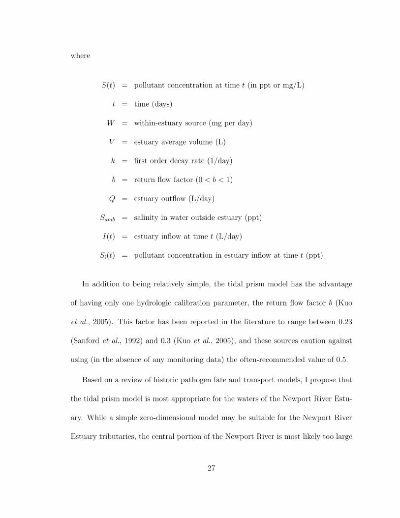
where
S(t) = pollutant concentration at time t (in ppt or mg/L)
t = time (days)
W = within-estuary source (mg per day)
V = estuary average volume (L)
k = first order decay rate (1/day)
b = return flow factor (0 < b < 1)
Q = estuary outflow (L/day)
Samb = salinity in water outside estuary (ppt)
I(t) = estuary inflow at time t (L/day)
Si(t) = pollutant concentration in estuary inflow at time t (ppt)
In addition to being relatively simple, the tidal prism model has the advantage
of having only one hydrologic calibration parameter, the return flow factor b (Kuo
et al., 2005). This factor has been reported in the literature to range between 0.23
(Sanford et al., 1992) and 0.3 (Kuo et al., 2005), and these sources caution against
using (in the absence of any monitoring data) the often-recommended value of 0.5.
Based on a review of historic pathogen fate and transport models, I propose that
the tidal prism model is most appropriate for the waters of the Newport River Estu-
ary. While a simple zero-dimensional model may be suitable for the Newport River
Estuary tributaries, the central portion of the Newport River is most likely too large
27

for representation by a zero-dimensional model with a single reference monitoring
point. The loading reduction requirements for Newport River Estuary tributaries
may therefore have to serve as a conservative guide for the loading reduction re-
quirements of the Estuary itself (if it is found to be in violation of water quality
standards). A graphical representation of my proposed aquatic fate and transport
model, including critical environmental processes and system variables related to a
tidal prism model, is included in figure 2.3.
Figure 2.3: Graphical representation of environmental processes and system vari-ables affecting aquatic fate and transport of fecal indicator organisms. Managementdecisions are indicated by boxes, and variables are represented by rounded nodes.
2.4 Summary
The comprehensive graphical model is developed by combining designated submodels
for each system component, however a model simplifying step adapted from Borsuk
et al. (2004), in which model variables which are not controllable, predictable, or
observable are removed from the network, results in the graphical network presented
28

in figure 2.4.
Figure 2.4: Comprehensive graphical network of fecal contamination in designatedresource waters. Management decisions are indicated by boxes, and variables arerepresented by rounded nodes.
29

Chapter 3
Developing and Applying a Simple
Bayesian Network Model
Note: the research in this Chapter appears in peer-reviewed conference proceedings
of the Water Environment Federation TMDL 2007 Specialty Conference in Bellevue,
Washington (Gronewold et al., 2007).
Fate and transport processes related to bacteriological contamination of recre-
ational and shellfish harvesting waters are complicated and often poorly-understood
with a broad range of historic modeling efforts and associated varying degrees of
success. Developing water quality models which reflect implicit causal relationships
between environmental phenomena, land use patterns, and surface water quality are
vital to the long-term success of the USEPA Total Maximum Daily Load (TMDL)
Program. In this Chapter, I develop and apply a simple Bayesian network model
intended to support fecal coliform TMDL assessments in shellfish harvesting waters.
System components are graphically presented and discussed as a critical initial step in
successful model development, followed by establishment of probabilistic relationships
between system components. The subsequent model, while only a simplified version
of the more comprehensive model expected to be developed after my dissertation, is
suggested as an innovative tool for successful implementation of future TMDLs for
microbial contaminants. I begin by describing context for this research along with
30

a technical description of Bayesian networks. A graphical model representing sys-
tem dynamics in shellfish harvesting waters is presented, followed by application of
a submodel with data from the Newport River Estuary in eastern North Carolina.
3.1 Background
The goal of the TMDL process is to determine the maximum pollutant loading which
can enter a water body without exceeding water quality standards (National Research
Council, 2001; Shen et al., 2005). Despite the complications associated with model-
ing the relationship between fecal indicator bacteria (FIB) loading, surface water FIB
concentrations, and ultimately shellfish contamination, shellfish harvesting resource
area managers are charged with protecting human health by closing harvesting areas
immediately following conditions which may increase the risk of exposure to water-
borne pathogens. Shellfish harvesting areas which violate long-term water quality
standards are placed on the USEPA 303(d) list of impaired waters and are required
to undergo a TMDL assessment. Simple models are therefore needed to simultane-
ously support short-term management programs while providing forecast information
which can guide long-term management actions towards water quality standard com-
pliance. Key characteristics of these simple models should include, but not be limited
to, appropriate acknowledgement of uncertainty (in all phases of the process) and ap-
plicability to thousands of shellfish harvesting areas for which a TMDL assessment
is required, but has not been initiated.
31
Local shellfishing resource area management plans contain conservative criteria
for shellfish growing area closures and openings in order to protect human and envi-
ronmental health. Closure criteria typically include the volume of recent precipitation
events, while reopening criteria may include a subjective analysis of the number of
days since the precipitation event, event intensity, and monitoring to confirm water
quality restoration. Although these criteria are based on historic relationships be-
tween stormwater runoff and high pathogen concentrations in receiving waters, the
implicit causal relationship between precipitation intensity, lag between precipitation
events, land use patterns, receiving water quality and subsequent shellfish contami-
nation is poorly understood. Because short-term protection of human health takes
priority over long-term restoration of impaired shellfishing areas, effective implemen-
tation of a shellfishing resource area management plan does not necessitate explicit
understanding of the runoff-contamination relationship. Current management prac-
tices reflect the assumption that precipitation-based responses in water quality are
similar within neighboring stations and closure decisions are often subsequently ap-
plied to large areas encompassing several stations.
Additional management scenarios in shellfish harvesting areas include short-term
closure and re-opening of resource areas under the authority of local management
agencies. The primary objective of local management scenarios, as opposed to the
long-term remediation goals of the TMDL program, is protecting human health
through restricting or prohibiting shellfish harvesting either during adverse pollution
32
conditions, such as a recent rainfall event, or due to long-term water quality standard
violations. Due to the close relationship between the criteria and environmental pro-
cesses related to these two management schemes, fecal pollution modeling strategies
need to be developed that address both public health concerns and retention and/or
restoration of the beneficial uses of the waterbody.
3.2 Bayesian Networks
A Bayesian network is a graphical representation of conditional probability distri-
butions relating a set of system variables coupled with their formal statistical and
probabilistic relationships (see Pearl, 1988; Spiegelhalter et al., 1993, for extensive
definitions). Qualitative assessment of graphical model structure represents the first
of three stages in the development of a Bayesian network model in which system vari-
ables and assumptions about their relationships are identified, and was discussed pre-
viously in Chapter 2 (Spiegelhalter et al., 1993). Each system variable in a Bayesian
network model is represented by a node, and the presence or absence of an arc between
nodes indicates conditional dependence or independence, respectively. Although arcs
between variable nodes typically imply causality in Bayesian networks, the condi-
tional dependence represented by an arc may indicate a more complex relationship
(Borsuk et al., 2004). The graphical model, while providing a framework for identi-
fying system variables and qualitative beliefs regarding their interdependence, does
not by itself carry a probabilistic interpretation (Spiegelhalter et al., 1993).
33

The second stage of Bayesian network model development acknowledges an im-
plicit joint probability distribution encompassing the proposed model variables and
reflecting the graphical structure of the network (Spiegelhalter et al., 1993). For ex-
ample, fecal contamination of coastal estuaries may be represented using a simple
model which relates rainfall distribution (R) to fecal coliform concentration (F ) as a
function of both non-point (N) and point source (P ) loading, as presented in figure
3.1.
Figure 3.1: Simple network model representing rainfall-induced fecal contaminationof a coastal estuary.
The joint probability of system variables in this simplified model can be written
via the chain rule as:
p(R, N, P, F ) = p(R)p(N |R)p(P |R, N)p(F |R, N, P )
The implied conditional independence indicated by the lack of an arc between
nodes allows us to simplify the joint probability to:
34

p(R, N, P, F ) = p(R)p(N |R)p(P |R)p(F |N, P )
This simplification is possible because once the direct causes of a system variable
are observed, other system variables do not influence understanding of the node’s
distribution (Spiegelhalter et al., 1993). The resulting joint probability can therefore
be viewed as a set of several local distributions, each made up of only a node and
its parents (Spiegelhalter et al., 1993; Borsuk et al., 2004). These local distributions,
commonly referred to as belief universes (see, e.g. Jensen et al., 1990), represent
the cornerstones of model decomposition and one of many benefits associated with
modeling an environmental system with a Bayesian network.
The third and final stage (Spiegelhalter et al., 1993) of Bayesian network model
development involves encoding the conditional probability distribution within the
graphical model structure. Conditional probability distributions are often established
using model simulations, in some cases combined with expert opinions on system
dynamics.
The Bayesian component of Bayesian network models addresses how new infor-
mation is used to modify the conditional probability relationships between system
variables in an existing model. Computations relating future conditional probabil-
ity relationships (posterior distributions) with previous or current understanding of
the relationships (prior distributions) and new observations (likelihood) are based on
Bayes’ theorem, which can be expressed as the following:
35

posterior ∝ likelihood × prior
A graphical representation of Bayes’ theorem is included in figure 3.2.
Figure 3.2: Graphical representation of Bayes’ theorem indicating prior and poste-rior probability densities, and the normalized likelihood for a water quality standard.
3.3 Methods
3.3.1 Study Area and Data Collection
The focus area for this study is the Newport River Estuary (NPRE), located along
the eastern coast of North Carolina in Carteret County. The Newport River and its
tributaries are collectively referred to as shellfish growing area E-4. Shellfish growing
36

area E-4 is locally managed by the North Carolina Department of Environment and
Natural Resources Shellfish Sanitation and Recreational Water Quality Section (SSS),
and encompasses forty individual harvesting areas currently included in USEPA’s
303(d) list of impaired waters targeted for TMDL assessment (see Appendix A)
Water quality samples from shellfish growing area E-4 are routinely collected by
SSS from 29 sampling stations in accordance with guidelines outlined by the National
Shellfish Sanitation Program Food and Drug Administration and Interstate Shellfish
Sanitation Conference (2005). Routine compliance samples are collected roughly
5 to 6 times per year, while adverse condition samples are collected after rainfall
events in order to determine the duration of short-term shellfish harvesting area
closings. The primary data set used for this analysis is the routine monitoring data. In
addition to analyzing samples for fecal coliform concentration, the approximate status
of the tide is recorded during each sampling event. Stations are periodically added to
and removed from the sampling program depending on monitoring needs. The SSS
monitoring data is the longest continuing dataset using consistent station locations
for bacteriological water quality information in the Newport River Estuary and is
the primary source of inference for determining water quality standard violations
and TMDL modeling efforts. Rainfall data within the Newport River Estuary is
obtained from the National Oceanographic and Atmospheric Association’s (NOAA)
national climatic data center (NCDC) weather observation station in Morehead City,
North Carolina.
37

3.3.2 Model Variables
A comprehensive graphical model representing assumed processes and system compo-
nents in a tidal shellfish harvesting area was developed in Chapter 2. Components of
the graphical model (see figure 3.3) were identified and related to one another based
on a review of historic studies of tidal estuary systems and guidance from USEPA
(Grant et al., 2001; Kashefipour et al., 2005; U.S. Environmental Protection Agency,
2001). Recent research indicates that a wide range of alternative indicator organisms
may reflect the health risks associated with fecal contamination, and therefore may be
considered as potential model endpoints (National Research Council, 2001). Such or-
ganisms include, but are not limited to, the family of coliform bacteria (which include
total coliform, fecal coliform, and Escherichia coli) and Enterococcus sp (U.S. Envi-
ronmental Protection Agency, 2001). Current guidelines for United States shellfish
harvesting waters indicate fecal coliform most probable number (MPN) and colony
forming unit (CFU) values as a basis for water quality standards.
For the purposes of this study, a simplified network model is derived from the
comprehensive model (figure 3.3) which includes only those variables which are mea-
surable, and which relate precipitation and tidal dynamics with fecal coliform MPN
measurements. Because water quality samples collected for this study were analyzed
by SSS using a 5-tube serial dilution multiple tube fermentation procedure resulting
in MPN estimates of fecal coliform concentration, fecal coliform MPN will serve as the
model endpoint. Exploratory analysis of historical data, local management criteria,
38

Figure 3.3: Graphical representation of environmental variables and processes as-sociated with fecal contamination in tidal shellfish harvesting areas. Managementdecisions are indicated by boxes, and variables are represented by rounded nodes.
and conversations with SSS personnel indicate precipitation and tide are two of the
most significant variables affecting bacteriological water quality within the Newport
River Estuary. A similar model simplification process is presented in Borsuk et al.
39

(2004).
In order to facilitate both graphical representation and Bayesian updating, I im-
plement the proposed model using the Bayesian network software package Neticar.
A critical aspect of implementing a Bayesian network model within most packaged
software programs is variable discretization, and variables in the proposed submodel
are primarily discretized in order to best reflect current local and federal management
criteria. For example, shellfish harvesting areas in the Newport River Estuary are
often closed after a daily rainfall event exceeding one inch. The magnitude of the
most recent rainfall event is therefore selected as a submodel variable with alternative
states of less than one inch and at least one inch. In addition, the shellfish manage-
ment guidelines outlined in Title 15A of the North Carolina Administrative Code
(NCAC), Chapter 18 (Environmental Health), SubChapter A (Sanitation), Sections
.0300 through .0900 (see Appendix B) indicate that the median fecal coliform most
probable number (MPN) or the geometric mean MPN of water shall not exceed 14
organisms per 100 ml, and not more than ten percent of the samples shall exceed
a fecal coliform MPN of 43 organisms per 100 ml (based on the five-tube serial di-
lution analysis procedure used by SSS). A graphical representation of the proposed
submodel, indicating the selected variables and their states, is included as figure 3.4.
Each node in figure 3.4 represents a system variable, and the rows within each node
indicate a variable state along with the associated probability distribution. Where
applicable, the bottom of each node includes the node variable mean and standard
40

Figure 3.4: Graphical submodel relating precipitation events, tidal dynamics, andwater quality. Probabilities for all variable states are based on monitoring datacollected between 1994 and 1997 at a cluster of monitoring stations in the upperreaches of the Newport River Estuary, North Carolina.
deviation. The values in figure 3.4 are based on water quality data collected from
monitoring stations in the upper reaches of the Newport River between 1994 and
1997.
3.3.3 Conditional Probabilities
Representing relationships between variables using conditional probability distribu-
tions facilitates not only model updating (using Bayes’ theorem), but also analysis of
sensitivity of the response variable (fecal coliform MPN) to alternative environmental
states. For example, the probability distributions expressed in figure 3.4 are based
on precipitation and tidal conditions only at the time of sampling. It is therefore
uncertain if the distribution of fecal coliform MPN presented in figure 3.4 is an ap-
propriate indicator of long-term average conditions in the water body and if it can
be used as an accurate tool for assessing impairment of the designated use.
41

Historic data from the Morehead City NCDC station for this time period indi-
cates that there are between 0 and 4 days of dryness between rainfall events roughly
84% of the time, and more than 4 days of dryness between rainfall events 16% of
the time. Historic data analysis also indicates that the magnitude of daily rainfall
events is less than 1 inch approximately 90% of the time. Adjusting the distribution
of environmental variables to reflect long term conditions provides a better under-
standing of the long-term distribution of the water quality measurement. Neticar
stores relationships between causal and response variables in a conditional proba-
bility table. In this example, the relationship between variables does not change as
we modify marginal probability distributions of (assumed) causal variables. Using
the chain rule, we can demonstrate how Neticar calculates the marginal probabil-
ity distribution for any state of the fecal coliform MPN given different states of the
causal variables. For example, figure 3.5 (from the Neticar graphical user inter-
face) shows the empirically-based conditional probability distribution table for fecal
coliform MPN. Each row corresponds to the conditional probability that the fecal
coliform MPN will be in a given state given the state of all three causal variables.
For example, the first row of the table indicates that there is a 0.67 probability that
the fecal coliform MPN will be below 14 organisms per 100 ml when the tide is rising,
when the most recent rainfall is less than one inch, and when the most recent rainfall
event was less than four days ago. Using the chain rule, the marginal probability
that the fecal coliform MPN is between 0 and 14 organisms per 100 ml (integrated
42

over all possible states the three causal variable states, expressed here as x1, x2, x3)
can be written as:
p(0 ≤ MPN < 14) =∑
X
p(0 ≤ MPN < 14 | x1, x2, x3)π(x1, x2, x3) (3.1)
We assume that x1, x2, x3 are independent, and can therefore rewrite equation 3.1
as:
p(0 ≤ MPN < 14) =∑
X
p(0 ≤ MPN < 14 | x1, x2, x3)π(x1)π(x2)π(x3)
We can then combine the conditional probabilities for the fecal coliform MPN in
figure 3.5 with any set of marginal probabilities of environmental (causal) variables.
The marginal probability that the fecal coliform MPN is between 0 and 14 organisms
per 100 ml under long-term environmental conditions (which, as stated previously,
are slightly different than those under which the samples were collected) is:
43

Figure 3.5: Conditional probability distribution table for fecal coliform MPN node.For each of the three states of the MPN node, each row indicates the marginalprobability of the node being in that state given the state of the three causal variables.For example, the probability that the MPN is less than 14 organisms per 100 ml, giventhat the tide is rising, the most recent rainfall was less than one inch, and that it hasbeen less than four days since the most recent rain event, is 0.667.
p(0 ≤ MPN < 14) =∑
X
p(0 ≤ MPN < 14 | x1, x2, x3)π(x1)π(x2)π(x3)
= (0.67)(0.90)(0.50)(0.84) +
(0.55)(0.90)(0.50)(0.16) +
(0.33)(0.10)(0.50)(0.84) +
(0.33)(0.10)(0.50)(0.16) +
(0.61)(0.90)(0.50)(0.84) +
(0.60)(0.90)(0.50)(0.16) +
(0.33)(0.10)(0.50)(0.84) +
(0.55)(0.10)(0.50)(0.16)
= 0.60
44

A summary of marginal distributions for each causal variable revised to reflect
long-term conditions in the Newport River Estuary, along with the revised marginal
distribution for the fecal coliform MPN, is presented in figure 3.6.
Figure 3.6: Graphical submodel relating precipitation events, tidal dynamics, andwater quality. Probabilities for fecal coliform MPN states are conditional uponlong-term average precipitation and tidal conditions in the upper reaches of the New-port River Estuary, North Carolina.
3.4 Results and Discussion
Results of the analysis of the conditional probability distributions of water quality
data within the upper reaches of the Newport River between 1994 and 2004 using
the proposed Bayesian network submodel are presented in table 3.1. The summary
table divides the data into three time periods, and indicates distribution of fecal
colifom MPN under the conditions at the time of sampling (e.g. figure 3.4) and ad-
justed for long-term average conditions (e.g. figure 3.6). Analysis of the data in table
3.1 indicates little change in the probability distribution of fecal coliform between
the selected time periods and between the long-term average distribution and the
45
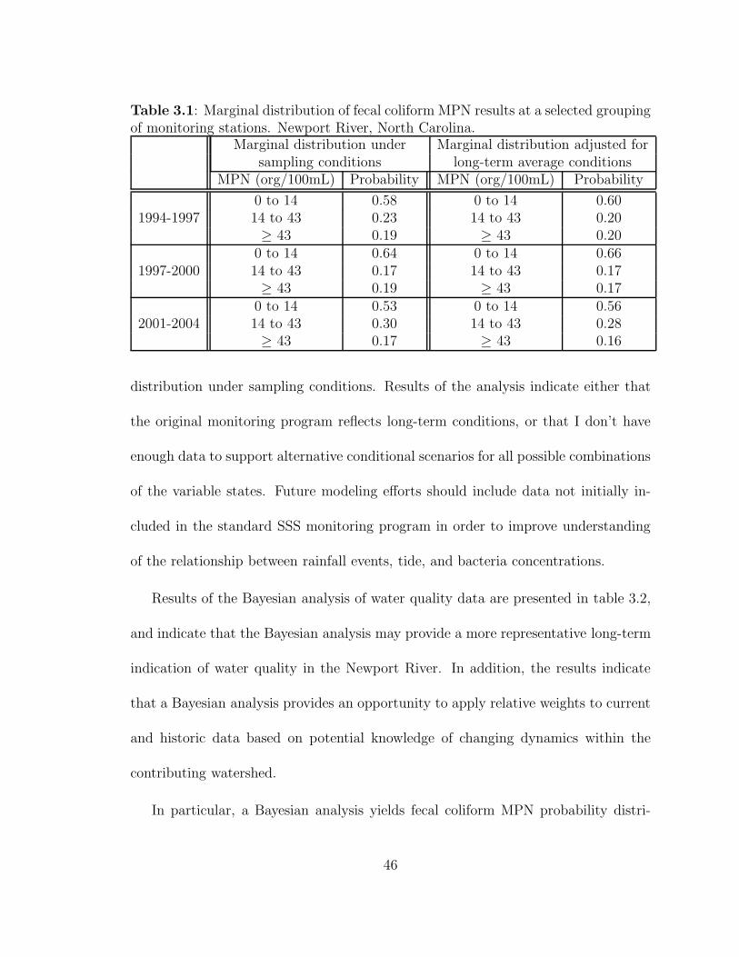
Table 3.1: Marginal distribution of fecal coliform MPN results at a selected groupingof monitoring stations. Newport River, North Carolina.
Marginal distribution under Marginal distribution adjusted forsampling conditions long-term average conditions
MPN (org/100mL) Probability MPN (org/100mL) Probability
0 to 14 0.58 0 to 14 0.601994-1997 14 to 43 0.23 14 to 43 0.20
≥ 43 0.19 ≥ 43 0.200 to 14 0.64 0 to 14 0.66
1997-2000 14 to 43 0.17 14 to 43 0.17≥ 43 0.19 ≥ 43 0.17
0 to 14 0.53 0 to 14 0.562001-2004 14 to 43 0.30 14 to 43 0.28
≥ 43 0.17 ≥ 43 0.16
distribution under sampling conditions. Results of the analysis indicate either that
the original monitoring program reflects long-term conditions, or that I don’t have
enough data to support alternative conditional scenarios for all possible combinations
of the variable states. Future modeling efforts should include data not initially in-
cluded in the standard SSS monitoring program in order to improve understanding
of the relationship between rainfall events, tide, and bacteria concentrations.
Results of the Bayesian analysis of water quality data are presented in table 3.2,
and indicate that the Bayesian analysis may provide a more representative long-term
indication of water quality in the Newport River. In addition, the results indicate
that a Bayesian analysis provides an opportunity to apply relative weights to current
and historic data based on potential knowledge of changing dynamics within the
contributing watershed.
In particular, a Bayesian analysis yields fecal coliform MPN probability distri-
46

Table 3.2: Summary of Bayesian analysis results for Newport River, North Carolinafecal coliform MPN data.
Prior distribution Posterior distributionMPN (org/100mL) Probability MPN (org/100mL) Probability
0 to 14 0.33(2) 0 to 14 0.611994-1997 14 to 43 0.33(2) 14 to 43 0.20
≥ 43 0.33(2) ≥ 43 0.190 to 14 0.61 0 to 14 0.64
1997-2000 14 to 43 0.20 14 to 43 0.18≥ 43 0.19 ≥ 43 0.18
0 to 14 0.64 0 to 14 0.622001-2004 14 to 43 0.18 14 to 43 0.22
≥ 43 0.18 ≥ 43 0.16NOTES: 1) All distributions conditional on long-term average conditions.
2) A very low relative weight (effective sample size = 1) was appliedto this prior distribution. See text for additional details.
butions at the end of each selected time period (i.e. 1994-1997, 1997-2000, and
2000-2004) with less between-time-period variance than the marginal probability dis-
tributions. For example, the marginal probability that fecal coliform MPN is below
14 is 0.56 for the 2000-2004 period compared to 0.66 to the 1997-2000 period (see
table 3.1). The Bayesian posterior probability that fecal coliform MPN is below 14
following the 2001-2004 time period is 0.62, compared to 0.64 for the 1997-2000 time
period (see table 3.2). These results imply that a Bayesian analysis is less influ-
enced by potential anomalies in the sampling data from a particular time period,
and perhaps provides a better overall representation of conditions within the water
body.
In addition, Bayesian analysis using the Neticar software allows prior and like-
lihood information to be weighted in order to reflect possible knowledge that either
47

historical or current data may serve as a more accurate indication of conditions as-
sessed for regulatory compliance. As an example, the prior probability distributions
presented for the 1994-1997 time period in table 3.2 are intended to reflect complete
ignorance of water quality conditions. A typical Bayesian analysis would reflect this
ignorance through an improper uniform prior distribution, applying equal probability
to all possible values of the fecal coliform MPN. In Neticar, a uniform probability
is applied using equal probabilities for all categories of the selected variable. As a
result, the prior distribution in table 3.2 for the 1994-1997 time period contains a
probability of 0.33 for each variable state. In order to minimize the effect of applying
disproportionate prior probabilities to each of the possible values of the fecal coliform
MPN, I apply a relative weight of 1 (i.e. relative sample size = 1) to the prior dis-
tribution allowing the likelihood (with a sample size of roughly 90) to dominate the
posterior distribution.
3.5 Conclusions
I have presented a case study applying conditional probability networks and Bayesian
updating to evaluate short and long-term water quality conditions within the Newport
River Estuary in North Carolina. This case study is intended to support the ongoing
evaluation of fecal contamination in the Newport River, and to serve as a precedent
for other water quality assessments conducted through the USEPA TMDL program.
A noted advantage to evaluating fecal contamination with a Bayesian network
48
model is the ability to easily adjust conditional probability distributions based on
changing knowledge of existing environmental conditions, and integration of new ev-
idence from ongoing and future water quality monitoring programs. The proposed
submodel serves as a template for a more rigorous analysis using the full comprehen-
sive Bayesian network model presented in figure 3.3. This research also suggests that
the current sampling scheme represents well the marginal probability distributions of
dominant environmental factors (e.g. wind and tide).
49

Chapter 4
An Assessment of Fecal IndicatorBacteria-Based Water Quality Standards
and Water Quality Model Endpoints
The content of this Chapter is published in Gronewold et al. (2008) and is available
at doi: 10.1021/es703144k. By permission of the American Chemical Society, the
abstract, figures, and tables are included below.
Abstract
Fecal indicator bacteria (FIB) are commonly used to assess the threat of pathogen
contamination in coastal and inland waters. Unlike most measures of pollutant lev-
els however, FIB concentration metrics, such as most probable number (MPN) and
colony-forming units (CFU), are not direct measures of the true in situ concentration
distribution. Therefore, there is the potential for inconsistencies among model and
sample-based water quality assessments, such as those used in the Total Maximum
Daily Load (TMDL) program. To address this problem, we present an innovative
approach to assessing pathogen contamination based on water quality standards that
impose limits on parameters of the actual underlying FIB concentration distribution,
rather than on MPN or CFU values. Such concentration-based standards link more
explicitly to human health considerations, are independent of the analytical proce-
50

dures employed, and are consistent with the outcomes of most predictive water quality
models. We demonstrate how compliance with concentration-based standards can be
inferred from traditional MPN values using a Bayesian inference procedure. This
methodology, applicable to a wide range of FIB-based water quality assessments, is
illustrated here using fecal coliform data from shellfish harvesting waters in the New-
port River Estuary, North Carolina. Results indicate that areas determined to be
compliant according to the current methods-based standards may actually have an
unacceptably high probability of being in violation of concentration-based standards.
Table 4.1: NSSP shellfish harvesting area fecal coliform water quality standardsbased on a minimum of 30 randomly collected samples.
Basis for standard Standardq50 µgeo q90
n MPN observations from 5-tube MTF procedure 14 14 43n CFU observations from MF procedure 14 14 31
µc 0.00 0.05 0.10 0.15 0.20 0.25 0.30 0.35 0.40 0.45 0.50 0.55σc 2.03 1.99 1.96 1.92 1.91 1.86 1.83 1.82 1.78 1.72 1.72 1.70µc 0.60 0.65 0.70 0.75 0.80 0.85 0.90 0.95 1.00 1.05 1.10 1.15σc 1.67 1.64 1.60 1.58 1.53 1.51 1.47 1.41 1.41 1.36 1.33 1.31µc 1.20 1.25 1.30 1.35 1.40 1.45 1.50 1.55 1.60 1.65 1.70 1.75σc 1.28 1.23 1.21 1.17 1.12 1.09 1.05 1.03 0.98 0.94 0.90 0.88µc 1.80 1.85 1.90 1.95 2.00 2.05 2.10 2.15 2.20 2.25 2.30 2.32σc 0.83 0.80 0.74 0.72 0.68 0.62 0.57 0.52 0.46 0.38 0.25 0.10
Table 4.2: Values of µc and σc constituting MPN contour line (for simulated violationfrequency = 0.005).
51

µc 0.00 0.05 0.10 0.15 0.20 0.25 0.30 0.35 0.40 0.45σc 1.93 1.91 1.85 1.83 1.81 1.79 1.75 1.72 1.70 1.67µc 0.50 0.55 0.60 0.65 0.70 0.75 0.80 0.90 0.95 1.00σc 1.63 1.60 1.57 1.54 1.52 1.47 1.44 1.38 1.33 1.31µc 1.05 1.10 1.15 1.20 1.25 1.30 1.40 1.45 1.50 1.55σc 1.28 1.24 1.21 1.20 1.14 1.10 1.05 1.02 0.98 0.94µc 1.60 1.65 1.70 1.75 1.80 1.85 1.90 1.95 2.00 2.05σc 0.92 0.90 0.85 0.82 0.80 0.76 0.72 0.71 0.66 0.62µc 2.10 2.15 2.20 2.25 2.30 2.35 2.40 2.45 2.50 2.51σc 0.61 0.57 0.53 0.51 0.48 0.42 0.35 0.26 0.12 0.05
Table 4.3: Values of µc and σc constituting CFU contour line (for simulated violationfrequency = 0.005).
Prior α β E(σk) V(σk)σk ∼ Un(α, β) 0 100 50 833.33φk ∼ Ga(α, β) 1.5 0.375 0.69 0.27φk ∼ Ga(α, β) 1.0 2.0 2.5 ∞
Table 4.4: Alternative priors for true concentration ck standard deviation σk atstation k.
standard σc range γ β0 β1
MPN >0.65 1.39 2.65 -1.04MPN ≤0.65 2.61 2.44 -1.05CFU >0.65 1.03 1.98 -0.66CFU ≤0.65 2.61 1.65 -0.66
Table 4.5: Regression model parameters including transformation parameter (γ),intercept (β0), and slope (β1).
52

σ
Density
0.0
0.5
1.0
1.5
2.0
2.5
3.0
01234
prio
rpo
ster
ior
σ≈
U(α
=0,
β=
100)
σ
Density
0.0
0.5
1.0
1.5
2.0
2.5
3.0
01234
prio
rpo
ster
ior
σ=
1φ,
φ
≈Γ(
α=
1.5,
β=
0.37
5)
σ
Density
0.0
0.5
1.0
1.5
2.0
2.5
3.0
01234
prio
rpo
ster
ior
σ=
1φ,
φ
≈Γ(
α=
1, β
=2)
σDensity
0.0
0.5
1.0
1.5
2.0
2.5
3.0
01234
prio
rpo
ster
ior
σ≈
U(α
=0,
β=
100)
σ
Density
0.0
0.5
1.0
1.5
2.0
2.5
3.0
01234
prio
rpo
ster
ior
σ=
1φ,
φ
≈Γ(
α=
1.5,
β=
0.37
5)
σ
Density
0.0
0.5
1.0
1.5
2.0
2.5
3.0
01234
prio
rpo
ster
ior
σ=
1φ,
φ
≈Γ(
α=
1, β
=2)
σ
Density
0.0
0.5
1.0
1.5
2.0
2.5
3.0
01234
prio
rpo
ster
ior
σ≈
U(α
=0,
β=
100)
σ
Density
0.0
0.5
1.0
1.5
2.0
2.5
3.0
01234
prio
rpo
ster
ior
σ=
1φ,
φ
≈Γ(
α=
1.5,
β=
0.37
5)
σ
Density
0.0
0.5
1.0
1.5
2.0
2.5
3.0
01234
prio
rpo
ster
ior
σ=
1φ,
φ
≈Γ(
α=
1, β
=2)
σ
Density
0.0
0.5
1.0
1.5
2.0
2.5
3.0
01234
prio
rpo
ster
ior
σ≈
U(α
=0,
β=
100)
σ
Density
0.0
0.5
1.0
1.5
2.0
2.5
3.0
01234
prio
rpo
ster
ior
σ=
1φ,
φ
≈Γ(
α=
1.5,
β=
0.37
5)
σ
Density
0.0
0.5
1.0
1.5
2.0
2.5
3.0
01234
prio
rpo
ster
ior
σ=
1φ,
φ
≈Γ(
α=
1, β
=2)
σ
Density
0.0
0.5
1.0
1.5
2.0
2.5
3.0
01234
prio
rpo
ster
ior
σ≈
U(α
=0,
β=
100)
σ
Density
0.0
0.5
1.0
1.5
2.0
2.5
3.0
01234
prio
rpo
ster
ior
σ=
1φ,
φ
≈Γ(
α=
1.5,
β=
0.37
5)
σ
Density
0.0
0.5
1.0
1.5
2.0
2.5
3.0
01234
prio
rpo
ster
ior
σ=
1φ,
φ
≈Γ(
α=
1, β
=2)
Fig
ure
4.1
:P
rior
and
pos
teri
ordis
trib
uti
ons
for
σk
for
five
random
lyse
lect
edst
atio
ns
inth
eN
ewpor
tR
iver
usi
ng
the
thre
epri
ors
inta
ble
4.4.
Eac
hro
wuti
lize
sth
esa
me
pri
ordistr
ibuti
on,
and
each
colu
mn
repre
sents
ase
par
ate
stat
ion.
Ver
tica
lgr
aylines
are
added
tofa
cilita
teco
mpar
ison
bet
wee
nal
tern
ativ
epri
ors
for
each
stat
ion.
53

a)
µc
σ c
0.0 0.5 1.0 1.5 2.0 2.5 3.0
0.0
0.5
1.0
1.5
2.0
2.5
Analytical Procedure
MPNCFU
b)
µc
σ c
0.0 0.5 1.0 1.5 2.0 2.5 3.0
0.0
0.5
1.0
1.5
2.0
2.5
Analytical Procedure
MPNCFU
c)
µc
σ c
0.0 0.5 1.0 1.5 2.0 2.5 3.0
0.0
0.5
1.0
1.5
2.0
2.5
Analytical Procedure
MPNCFU
d)
µc
σ c
0.0 0.5 1.0 1.5 2.0 2.5 3.0
0.0
0.5
1.0
1.5
2.0
2.5
Analytical Procedure
MPNCFU
Figure 4.2: Combinations of the mean µc and standard deviation σc of the log-trans-formed fecal coliform concentration distribution which yielded MPN (solid lines) orCFU (dashed lines) samples in violation of the NSSP median standard (panel a), ge-ometric mean standard (panel b), 90th percentile standard (panel c), or any standard(panel d) with a frequency of either 0.005 or 0.1. The zone of violations is in theupper right of each panel.
54
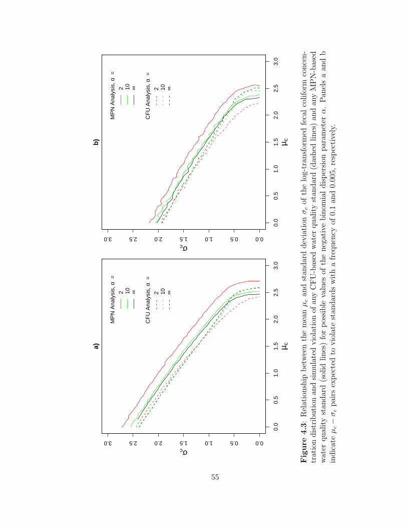
a) µ c
σc
0.0
0.5
1.0
1.5
2.0
2.5
3.0
0.00.51.01.52.02.53.0
MP
N A
naly
sis,
=
2 10 ∞
CF
U A
naly
sis,
=
2 10 ∞
α α
b) µ c
σc0.
00.
51.
01.
52.
02.
53.
0
0.00.51.01.52.02.53.0
MP
N A
naly
sis,
=
2 10 ∞
CF
U A
naly
sis,
=
2 10 ∞
α α
Fig
ure
4.3
:R
elat
ionsh
ipbet
wee
nth
em
ean
µc
and
stan
dar
ddev
iati
onσ
cof
the
log-
tran
sfor
med
feca
lco
lifo
rmco
nce
n-
trat
ion
dis
trib
uti
onan
dsi
mula
ted
vio
lati
onof
any
CFU
-bas
edw
ater
qual
ity
stan
dar
d(d
ashed
lines
)an
dan
yM
PN
-bas
edw
ater
qual
ity
stan
dar
d(s
olid
lines
)fo
rpos
sible
valu
esof
the
neg
ativ
ebin
omia
ldis
per
sion
par
amet
erα.
Pan
els
aan
db
indic
ate
µc−
σc
pai
rsex
pec
ted
tovio
late
stan
dar
ds
wit
ha
freq
uen
cyof
0.1
and
0.00
5,re
spec
tive
ly.
55

−2 0 2 4 6
−50
050
100
a)
γ
log−
likel
ihoo
d
−2 0 2 4 6
−10
010
2030
b)
γlo
g−lik
elih
ood
−2 0 2 4 6
−50
050
100
c)
γ
log−
likel
ihoo
d
−2 0 2 4 6
−20
010
2030
d)
γ
log−
likel
ihoo
d
Figure 4.4: Log-likelihood (solid line) of transformation parameter γ for σc usingpaired values of µc and σc. Panel a based on values from table 4.2 for σc > 0.65,panel b based on values from table 4.2 for σc ≤ 0.65, panel c based on values fromtable 4.3 for σc > 0.65, and panel d based on values from table 4.3 for σc ≤ 0.65.
56

µc
σ c
0.0 0.5 1.0 1.5 2.0 2.5
0.0
0.5
1.0
1.5
2.0
Violation frequency contour lines
MPNCFU
Model fit
MPNCFU
σc = 0.65
Figure 4.5: Violation contour lines overlaid by violation line best-fit regressionmodel fitted values based on model parameters in table 4.5.
57

CC (%) Posterior probability of Violated any MPN standardStn. MPN CFU size-30 sample violating during the 2000–2005
any MPN standard assessment period?3 52 39 5 no4 44 33 6 no
4A <1 <1 53 yes4B <1 <1 85 yes5A <1 <1 80 yes7 <1 <1 55 yes8 14 9 18 no
8A 15 12 15 no9 93 89 <1 no10 100 100 <1 no11 53 41 5 no
14A 51 40 6 no16A 32 20 12 no18 62 50 3 no24 80 71 1 no25 3 2 32 no
27A <1 <1 49 yes28 96 93 <1 no29 <1 <1 58 yes35 80 73 1 no41 <1 <1 89 yes
41A <1 <1 72 yes55 60 49 4 no56 78 67 1 no83 47 35 5 no84 13 6 17 no85 94 91 <1 no86 87 81 1 no
Table 4.6: Estimated confidence of compliance (CC), posterior probability of vi-olating any MPN standard, and observed violations for monitoring stations in theNewport River Estuary during the 2000-2005 assessment period.
58

Station 25
µc
σ c
0.0 0.5 1.0 1.5 2.0 2.5 3.0
0.0
0.5
1.0
1.5
2.0
2.5
Probability density contour linesMPN 0.5% violation standardCFU 0.5% violation standard
CC = 2−3%
Station 27A
µc
σ c
0.0 0.5 1.0 1.5 2.0 2.5 3.0
0.0
0.5
1.0
1.5
2.0
2.5
Probability density contour linesMPN 0.5% violation standardCFU 0.5% violation standard
CC < 1%
Station 3
µc
σ c
0.0 0.5 1.0 1.5 2.0 2.5 3.0
0.0
0.5
1.0
1.5
2.0
2.5
Probability density contour linesMPN 0.5% violation standardCFU 0.5% violation standard
CC = 39−52%
Station 35
µc
σ c
0.0 0.5 1.0 1.5 2.0 2.5 3.0
0.0
0.5
1.0
1.5
2.0
2.5
Probability density contour linesMPN 0.5% violation standardCFU 0.5% violation standard
CC = 73−80%
Figure 4.6: Joint posterior probability density contour lines (solid lines) for fourmonitoring stations in the Newport River Estuary. Dashed lines indicate combina-tions of the mean µc and standard deviation σc of the log-transformed fecal coliformconcentration distribution which violate concentration-based standards no more than0.5% of the time using MPN or CFU standards as the reference. Confidences of com-pliance (CC) are given in the lower left of each panel for both MPN and CFU-basedstandards.
59

Chapter 5
Modeling the Relationship Between Most
Probable Number (MPN) and Colony
Forming Unit (CFU) Estimates of Fecal
Indicator Bacteria Concentrations
Reproduced in part with permission from Gronewold and Wolpert (2008). Copyright
2008 Elsevier. Available at doi:10.1016/j.watres.2008.04.011
Most probable number (MPN) and colony-forming-unit (CFU) estimates of fe-
cal coliform bacteria concentration are common measures of water quality in coastal
shellfish harvesting and recreational waters. Estimating procedures for MPN and
CFU have intrinsic variability and are subject to additional uncertainty arising from
minor variations in experimental protocol. It has been observed empirically that the
standard multiple-tube fermentation (MTF) decimal dilution analysis MPN proce-
dure is more variable than the membrane filtration CFU procedure, and that MTF-
derived MPN estimates are somewhat higher on average than CFU estimates, on
split samples from the same water bodies. I construct a probabilistic model that
provides a clear theoretical explanation for the variability in, and discrepancy be-
tween, MPN and CFU measurements. I then compare my model to water quality
samples analyzed using both MPN and CFU procedures, and find that the (often
large) observed differences between MPN and CFU values for the same water body
60

are well within the ranges predicted by my probabilistic model. Results indicate that
MPN and CFU intra-sample variability does not stem from human error or labora-
tory procedure variability, but is instead a simple consequence of the probabilistic
basis for calculating the MPN. These results demonstrate how probabilistic models
can be used to compare samples from different analytical procedures, and to deter-
mine whether transitions from one procedure to another are likely to cause a change
in quality-based management decisions.
5.1 Introduction
Coastal water resource management agencies frequently revise standard water qual-
ity analysis procedures based on the latest available technologies. For example, the
North Carolina Department of Environmental and Natural Resources Shellfish San-
itation and Recreational Water Quality Section (NCDENR-SSS), and similar water
resource management agencies, are considering replacing multiple-tube fermentation
(MTF) fecal coliform analysis procedures with membrane filtration (MF) procedures
because MF results, while variable, are much less so than MTF results (as commonly
implemented) from the same water quality sample. NCDENR-SSS and other agen-
cies are concerned, however, that water quality-based management decisions for a
particular water body (such as approval or prohibition of shellfishing) may change
after MF procedures are implemented.
Here, I derive a theoretical model for the probability distribution of MTF and MF
61

test results from the same water quality sample. This innovative approach allows a
side-by-side comparison of alternative testing methods, accommodating their intrinsic
differences (rather than assuming that these differences have no effect). Further, I
find the probability distributions for the true fecal coliform concentrations associated
with different possible measurement results from each procedure.
Differences, if observed, between the MTF-MF relationship predicted by my model
and the MTF-MF relationship observed empirically in samples from a particular
laboratory, would suggest significant extrinsic sources of uncertainty and variability
(i.e. unrelated to natural spatial distribution of organisms in a sample aliquot volume)
and, more importantly, an increased chance that changing standard fecal coliform
analysis from MTF to MF might lead to a change in water quality-based management
decisions.
Variability in MTF and MF analysis results can be divided into two categories:
intrinsic stochastic variability due to the natural dispersion of bacteria within sample
containers, and extrinsic variability. Intrinsic sources of variability are mostly a
consequence of procedure design, and are explained later in this section. Extrinsic
sources of variability include departures from expected sampling protocol, microbial
cell damage (during filtration, for example) which may reduce the number of viable
organisms (Kloot et al., 2006), and clumping of bacteria cells (Noble et al., 2003b).
Other potential extrinsic sources of variability relate to environmental conditions
at the time of sampling, including antecedent rainfall, turbidity, and season (Cabelli
62

et al., 1983; Noble et al., 2003a). These extrinsic sources of variability are not included
in my model and, if they actually contribute to MTF-MF intra-sample variability,
will limit my model’s ability to explain the difference between MTF and MF results.
Fecal and total coliform bacteria are indicators of potential fecal pollution and
water-borne pathogenic threats to human health (Cabelli, 1983; LeClerc et al., 2001).
Other bacterial measures of water quality include Escherichia coli (a subset of fecal
coliforms), and enterococci (Noble et al., 2003a). Extensive definitions of fecal and
total coliform bacteria are presented elsewhere (Rompre et al., 2002; Kloot et al.,
2006). My model is applied to monitoring data from shellfish harvesting areas in
which fecal coliform is a more common measure of water quality. As a result, I
discuss only fecal coliform bacteria concentrations for the rest of this paper, however
the application of probabilistic models to intra-sample variability can be applied to a
wide range of microbial, physical, and chemical pollutants (see, e.g. Kinzelman et al.,
2003; U.S. Geological Survey, 1996; Horowitz, 1986).
MTF and MF are two common procedures for estimating fecal coliform concen-
trations in coastal resource waters (Eckner, 1998; Buckalew et al., 2006). MTF and
MF fecal coliform analysis results are reported as most probable number (MPN) and
colony-forming unit (CFU) estimates of the true fecal coliform concentration c (typ-
ically in organisms per 100 ml). Detailed descriptions of the MF microbial analysis
procedure are presented in Rose et al. (1975), Rippey et al. (1987), Dufour et al.
(1981), Eckner (1998), and Esham and Sizemore (1998). Similar descriptions of the
63

MTF procedure are presented in Cochran (1950); Hurley and Roscoe (1983); Beliaeff
and Mary (1993); McBride et al. (2003).
MPN estimates derived from a standard (e.g. 5-tube × 3 dilution series) MTF
analysis are, by definition, the possible values of the concentration at which the
likelihood function (see Appendix, equation 5.2) attains its maximum. The likelihood
function offers an indication of how strongly an observed pattern of positive tube
counts from an MTF analysis support each possible value c of the concentration
(McBride, 2005, pp. 12–13). The MPN estimates are highly variable because this
function has a very broad peak, and so is close to its maximum value over a wide
range of possible concentrations.
Additional discussion of the statistical assumptions inherent in MTF-based MPN
calculations can be found in Eisenhart and Wilson (1943); Beliaeff and Mary (1993);
Klee (1993). CFU estimates are based on the number of distinguishable bacterial
colonies which form on a culture plate after filtration and incubation. CFU variability
is inversely proportional to the volume of sample water filtered, and therefore while
CFU estimates are variable, the variability is often small compared to that of MTF-
derived MPN estimates when large aliquot volumes are used. The broad likelihood
function of MTF positive tube count observations and variability in the number of
distinguishable bacterial growth colonies are both examples of intrinsic variability in
MPN and CFU estimates, and are therefore addressed explicitly in my model.
Several recent studies document empirical relationships between fecal bacteria
64

analysis results from different testing procedures (e.g. Eckner, 1998; Noble et al.,
2003b; Kloot et al., 2006). The study by Noble et al. (2003b), for example, which
compares beach water quality analysis results using MF, MTF, and the IDEXX
Quanti-Tray R©/2000 chromogenic substrate test (CST) kit, indicates that measure-
ment error inherent to analytical procedures is likely to exceed differences between an-
alytical procedures assuming standard laboratory procedures are followed; Buckalew
et al. (2006) also find the intrinsic variability of these methods to exceed their differ-
ences.
Furthermore, Noble et al. (2003b) acknowledge that different test procedures are
likely to yield different fecal coliform concentration estimates because they measure
different metabolic process endpoints. Similar historic studies include a comparison
between MF-derived estimates of enterococci and E. coli by Levin et al. (1975) and
Dufour et al. (1981), a comparison between total coliform, fecal coliform, and fecal
streptococci concentration estimates using MTF procedures by Sayler et al. (1975),
and comparison between both MTF and MF estimates of E. coli, Klebsiella, and
Enterobacter species by Dufour and Cabelli (1975). I know of no study, however,
which attempts to explain the difference between standard MF and MTF procedures
by modeling only intrinsic variability in MPN and CFU estimates.
The remaining sections of this paper include a description of fecal coliform water
quality sampling and analysis procedures, followed by my approach to deriving a
probabilistic model of the relationship between observed MPN and CFU estimates.
65

I then present results of the analysis, including a comparison of my proposed theo-
retical probability distributions to observations from a recent NCDENR-SSS water
quality study which included analysis for fecal coliform concentration using both
MTF and MF procedures. I fit an ordinary least-squared (OLS) regression model to
the NCDENR-SSS data and compare regression model fitted values and prediction
intervals to my theoretical probability model. I conclude with a discussion of how my
findings might be used to guide water resource area management agencies through
transitions from one standard water quality analysis procedure to another.
5.2 Methods
5.2.1 Water Quality Monitoring
One-hundred and forty-four surface water quality samples were collected by NCDENR-
SSS personnel at monitoring stations throughout the Newport River Estuary in East-
ern North Carolina between May 2006 and January 2007 (NCDENR, 2007, unpub-
lished data). As a designated shellfish harvesting area, the Newport River Estuary
is governed by the National Shellfish Sanitation Program (NSSP) whose guidelines
(Food and Drug Administration and Interstate Shellfish Sanitation Conference, 2005)
require that its water quality standards be based on either MPN or CFU estimates of
fecal coliform bacteria concentration. Water quality samples were therefore analyzed
by NCDENR-SSS for fecal coliform concentration using both 5-tube decimal dilution
66

MTF and MF analysis tests in accordance with both NSSP guidelines and industry
standards (APHA, 2005).
5.2.2 Theoretical Probability Model
I derive a probabilistic model, addressing only intrinsic sources of variability, of the
relationship between fecal coliform MTF and MF measurements from the same water
quality sample. This model is theoretical because it assumes extrinsic sources of
variability are insignificant. I begin by calculating the probability distribution of the
MPN and CFU for any true fecal coliform concentration c (measured in organisms per
100 ml). I then implement a Bayesian analysis to derive the conditional distribution
of the true fecal coliform concentration c for any recorded MPN or CFU estimate.
Finally, I apply conditional probability distribution theory to yield the probability
function of the MPN for any observed CFU estimate from the same sample. Details
of the calculation procedures are included in the last section of this Chapter.
5.2.3 OLS Regression Empirical model
In addition to deriving a theoretical probability model, I fit a simple empirical log-
scale OLS regression model to the NCDENR-SSS data (see Weisberg, 2005, pp. 21–
30 for details on OLS regression). When all tubes in an MTF test are negative,
the maximum likelihood estimate (and hence the MPN) of the true concentration
c is zero (see Calculations section, equation 5.1). Because the logarithm of zero is
67

not finite, my regression model excludes 7 NCDENR-SSS data points with an MPN
of 0 organisms per 100 ml, and (for similar reasons) two data points with a CFU
of 0 organisms per 100 ml. The regression model also excludes the 19 NCDENR-
SSS observations whose MF test results were recorded as “too numerous to count
(TNTC)”.
5.3 Results and Discussion
In figure 5.1 I present expected values of the MPN (in panel A) and CFU (in panel B)
for every 5th integer-valued true fecal coliform concentration c in the range 0 ≤ c ≤
250, including 95% prediction sets. The 95% prediction set is the finite collection of
highest-probability values from a (perhaps multi-modal, as in the case of the MPN)
discrete probability distribution whose cumulative probability is at least 0.95. While
these sets are well-represented as intervals for the CFU in panel B, it is clear (see
panel A) that the likely MPN values vary widely and the 95% prediction sets are not
well-represented by continuous intervals. The results in figure 5.1 illustrate that the
wide variability of MPN results, a feature which might be misattributed to extrinsic
variability, is really a simple consequence of the probability distribution for the MPN.
In figure 5.2 I present expected values of the true fecal coliform concentration,
along with 95% credible intervals, for observable MPN estimates (in Panel A) and
for every 5th observable CFU estimate (in Panel B). A Bayesian 95% credible interval
contains the true fecal coliform concentration with a probability at least 0.95; see
68

Casella and Berger (2002, pp. 436–437) or McBride (2005, pp. 208–209), where credi-
ble intervals are described in detail and contrasted with confidence intervals. Details
of my Bayesian analysis are presented in the Calculations section. The “observable
MPN estimates” are those which can possibly arise from the (NSSP standard) 5-tube
fermentation serial dilution analysis (the most likely ones are presented, for example,
in tables in Woodward, 1957); for a sample aliquot volume of 100 ml (per NCDENR-
SSS operating protocol), the observable CFU estimates are all nonnegative integers.
Lengths of credible intervals depend on the numbers of tubes used, for MPN, and on
aliquot volume, for CFU (see Calculations, equation 5.5); thus, although the confi-
dence intervals for the CFU method are narrower than those for the MPN method
for any fixed sample volume (as suggested by the relative interval lengths in panels
A and B of figure 5.2), intervals could be made narrower for either method by using
more tubes (for MPN) or a greater volume (for CFU).
In figure 5.3 I present OLS regression model fitted values and theoretical probabil-
ity model expected values of the MPN for CFU estimates observed in the NCDENR-
SSS study. In addition, I present MPN 95% prediction intervals and prediction sets
for the regression model and probabilistic model, respectively. Observations from the
NCDENR-SSS study are also plotted in figure 5.3.
Prediction intervals in panel A of figure 5.3 are based on standard assumptions
regarding the distribution of OLS linear regression model fitted value residuals (see
Weisberg, 2005), and are presented to contrast with the true discrete multi-modal
69

distribution of the MPN presented in both panel B of figure 5.3, and in detail in figure
5.4. Figure 5.4 includes the full theoretical probability distribution of the MPN for
an observed CFU value of 6 organisms per 100 ml along with a histogram of MPN
estimates from 13 of the NCDENR-SSS water quality samples with a CFU estimate
of 6 organisms per 100 ml. Figures 5.3 and 5.4 demonstrate not only that the most
likely MPN estimates for a given water quality sample are a discrete subset of non-
consecutive observable MPN estimates, but also that the NCDENR-SSS observations
are entirely consistent with my theoretical probability model. Furthermore, my the-
oretical probability model explains why the MPN is a positively-biased estimate of
fecal coliform concentration (Garthright, 1993, 1997).
Despite differences between regression model fitted values (panel A of figure 5.3)
and expected values from my theoretical probability model (panel B of figure 5.3),
I expect empirical regression model fitted values to approach expected values of the
MPN for a specific CFU as sample size increases. Differences, if any, between large-
sample empirical regression model fitted values and my theoretical model expected
values might suggest significant non-probabilistic (i.e. extrinsic) sources of variabil-
ity. Exploring comparisons between my proposed probabilistic model and regression
models fit to very large data sets is an area for future research.
70

5.4 Conclusions
I derived a theoretical model of the MPN probability distribution for any observed
CFU estimate from the same water quality sample. Recent water quality samples
collected and analyzed by NCDENR-SSS for fecal coliform concentration using both
MTF and MF analysis tests yielded MPN and CFU estimates entirely consistent
with my theoretical probabilistic model. My results indicate that MPN and CFU
intra-sample variability does not stem from human error or laboratory procedure
variability, but is instead a simple consequence of the probabilistic basis for calculat-
ing the MPN.
I anticipate this study will serve as a stepping stone towards future research on
whether different fecal coliform analysis procedures might lead to different water
quality standard violation frequencies for the same water body. Method-dependent
differences, if any, might propagate into coastal resource water management decisions
through two undesirable pathways. First, analysis of water quality samples from a
coastal resource water might, depending on the analysis procedure used, result in
different management actions (such as closing or opening a shellfish harvesting area).
Second, if fecal coliform concentration estimates vary depending on whether MTF or
MF procedures are used, potential benefits of merging historic MPN and new CFU
data sets would be limited (Noble et al., 2003b). Future research on the probabilistic
basis for current water quality standard violations, coupled with the modeling tools
presented in this paper, could provide answers to these research questions.
71

Other suggested studies stemming from this research include, but are not limited
to, quantifying membrane filtration-related fecal coliform thinning and contamination
rates, exploring environmental effects on fecal coliform concentration estimate bias,
and determining how measuring different coliform bacteria metabolic output effects
fecal coliform concentration estimates.
5.5 Calculations
Assuming fecal coliform organisms at concentration c (in organisms per 100 ml) are
well mixed in a water sample, it is commonly assumed that aliquots of volume vi ml
from the water sample contain a Poisson Po(cvi/100) distributed number of fecal co-
liform organisms (McCrady, 1915; Greenwood and Yule, 1917; de Man, 1977; Russek
and Colwell, 1983; Best and Rayner, 1985; Woomer et al., 1990; Briones and Re-
ichardt, 1999). Out of ni serial dilution analysis tubes, the numbers of positive tubes
xi are independent binomial Bi(ni, pi) random variables with pi = 1− exp(−cvi/100)
(for more on using Poisson and binomial distributions in environmental data analysis,
see Ott, 1995, pp. 93–113 and 127–137). The MPN for m dilution series can therefore
be expressed as:
MPN = argmaxc
[
m∏
i=1
(
1 − e−cvi/100)xi
(
e−cvi/100)ni−xi
]
(5.1)
72

and the conditional probability distribution of positive tube counts X = {xi}, given
true fecal coliform concentration c, is:
f(x | c) =m∏
i=1
(
ni
xi
)
[
1 − e−cvi/100]xi
[
e−cvi/100]ni−xi
(5.2)
The Poisson-distributed CFU observation Y ∼ Po(λ) with mean λ = cV/100 for
sample aliquot volume V ml has conditional probability distribution, given true fecal
coliform concentration c, given by
f(y | c) =1
y!(cV/100)ye−cV/100 for y ∈ 0, 1, 2, . . . (5.3)
The posterior probability distribution of the true fecal coliform concentration c
for an observed tube count combination x, using Jeffreys’ scale-invariant “reference”
prior distribution π(c) ∝ 1/√
c (Jeffreys, 1946; Bernardo and Ramon, 1998), is given
by:
f(c | x) ∝ c−1/2e−(c/100)∑m
i=1 vi(ni−xi)m∏
i=1
(
1 − e−cvi/100)xi
, c > 0 (5.4)
Using the same Jeffreys’ prior distribution, the posterior distribution of c for a
73

given CFU observation y is:
f(c | y) ∝ cy−1/2e−cV/100, c > 0 (5.5)
which is a Gamma Ga(α, λ) distribution with shape parameter α = y + 1/2 and rate
parameter λ = V/100.
Finally I calculate the probability distribution of the positive tube count vector
x = (x1, . . . , xm), 1≤xi≤ni for any CFU observation y, P[X = x | Y = y], by
combining equations 5.2 and 5.5:
f(x | y) =
∫
∞
0
f(x | c)f(c | y)dc (5.6)
=(V/100)y+1/2
Γ(y + 1/2)×
∫
∞
0
cy−1/2e−(c/100)[V +∑m
i=1 vi(ni−xi)]m∏
i=1
(
ni
xi
)
(
1 − e−cvi/100)xi
dc.
74

050
100
150
200
250
02004006008001000
Tru
e fe
cal c
olifo
rm c
once
ntra
tion
(org
anis
ms
per
100
ml)
Fecal coliform MPN (organisms per 100 ml)
A
E(M
PN
|c)
MP
N 9
5% p
redi
ctio
n se
t for
spe
cifie
d tr
ue c
once
ntra
tion
1:1
line
050
100
150
200
250
02004006008001000T
rue
feca
l col
iform
con
cent
ratio
n (o
rgan
ism
s pe
r 10
0 m
l)Fecal coliform CFU (organisms per 100 ml)
E(C
FU
|c)
1:1
line
! M
PN
95%
pre
dict
ion
inte
rval
for
spec
ific
true
con
cent
ratio
n
B
Fig
ure
5.1
:E
xpec
ted
valu
esan
d95
%pre
dic
tion
sets
orpre
dic
tion
inte
rval
sfo
rob
serv
able
feca
lco
lifo
rmM
PN
(pan
elA
)an
dC
FU
(pan
elB
)m
easu
rem
ents
give
nth
etr
ue
feca
lco
lifo
rmco
nce
ntr
atio
nin
orga
nis
msper
100
ml.
For
clar
ity,
expec
ted
valu
esan
d95
%pre
dic
tion
sets
orin
terv
als
are
plo
tted
only
for
ever
y5th
inte
ger-
valu
edco
nce
ntr
atio
nc.
Max
imum
true
conce
ntr
atio
ns
inea
chplo
tar
ebas
edon
max
imum
MP
Nan
dC
FU
obse
rvat
ions
inth
eN
CD
EN
R-S
SS
dat
ase
t.C
FU
pre
dic
tion
inte
rval
sar
ebas
edon
anM
Fsa
mple
aliq
uot
volu
me
of10
0m
l.
75

050
100
150
200
250
02004006008001000
Fec
al c
olifo
rm M
PN
(or
gani
sms
per
100
ml)
True fecal coliform concentration (organisms per 100 ml)
A
E(c
|MP
N)
1:1
line
! 9
5% c
redi
ble
inte
rval
s
050
100
150
200
250
02004006008001000F
ecal
col
iform
CF
U (
orga
nism
s pe
r 10
0 m
l)True fecal coliform concentration (organisms per 100 ml)
E(c
|CF
U)
1:1
line
! 9
5% c
redi
ble
inte
rval
s
B
Fig
ure
5.2
:E
xpec
ted
valu
ean
d95
%cr
edib
lein
terv
als
forth
efe
calco
lifo
rmtr
ue
conce
ntr
atio
ngi
ven
MP
N(p
anel
A)an
dC
FU
(pan
elB
)es
tim
ates
inor
ganis
ms
per
100
ml.
For
clar
ity,
pan
elA
incl
udes
only
the
51ob
serv
able
MP
Nes
tim
ates
pre
sente
din
stan
dar
dla
bor
ator
yan
alysi
sM
TF
conve
rsio
nta
ble
sfo
rth
e5-
tube
seri
aldiluti
onan
alysi
spro
cedure
(see
,e.
g.W
oodw
ard,
1957
)an
dpan
elB
incl
udes
only
ever
y5th
obse
rvab
leC
FU
valu
ebas
edon
anM
Fte
stw
ith
asa
mple
aliq
uot
volu
me
of10
0m
l.
76

Fec
al c
olifo
rm C
FU
(or
gani
sms
per
100
ml)
Fecal coliform MPN (organisms per 100 ml)
!
NC
DE
NR
−S
SS
dat
a us
ed in
log−
linea
r re
gres
sion
mod
elN
CD
EN
R−
SS
S d
ata
excl
uded
from
log−
linea
r re
gres
sion
mod
elR
egre
ssio
n m
odel
fitte
d va
lues
95%
MP
N p
redi
ctio
n in
terv
al1:
1 lin
e
0125102050100200500
01
25
1020
5010
020
0
A
Fec
al c
olifo
rm C
FU
(or
gani
sms
per
100
ml)
Fecal coliform MPN (organisms per 100 ml)
NC
DE
NR
−S
SS
dat
aE
(MP
N|C
FU
)95
% M
PN
pre
dict
ion
set (
for
spec
ified
CF
U)
1:1
line
0125102050100200500
01
25
1020
5010
020
0
B
Fig
ure
5.3
:E
mpir
ical
linea
rre
gres
sion
model
(pan
elA
)an
dth
eore
tica
lpro
bab
ility
model
(pan
elB
)of
the
rela
tion
ship
bet
wee
nfe
calco
lifo
rmM
PN
and
CFU
esti
mat
esfr
omth
esa
me
wat
erqual
ity
sam
ple
.
77

0.00
0.05
0.10
0.15
0.20
0.25
0.30
0.35
MPN (organisms per 100 ml)
Pro
babi
lity
mas
s
Observed CFU = 6 organisms per 100 mlE(MPN|CFU = 6) = 7.6 organisms per 100 mlObserved MPN values when CFU = 6f(MPN|CFU=6)
01
23
4
0 1 5 10 20 50 100 200 500 1000
Num
ber
of o
bser
vatio
ns
Figure 5.4: Observed values, expected values, and the theoretical probability massfunction of the MPN for a CFU measurement from the same water quality sample.Observed values are from recent NCDENR-SSS study.
78

Chapter 6
Improving Parameter Estimation in the
Aquatic Fate and Transport Model
Much of the research in this chapter was completed in collaboration with Dr. Song
Qian, Dr. Robert Wolpert, Dr. Rachel Noble and Dr. Kenneth Reckhow, and was
submitted to Water Research.
Water resource management decisions often depend on mechanistic or empirical
models to predict water quality conditions under future pollutant loading scenarios.
While explicitly acknowledging process, observation, and analytical uncertainty in
these models is considered critical to model-based resource management decisions
and protection of human and environmental health, few tools have been developed
which explicitly propagate analytical uncertainty into fecal indicator bacteria (FIB)
water quality models. Here, I explore how ignorance or acknowledgement of model
input uncertainty affects model parameter estimates in a simple FIB water quality
model. I present two approaches to calibrating the model using simulated results
of a standard multiple-tube fermentation (MTF) serial dilution analysis. The first
approach uses only the most probable number (MPN) point estimate, while the sec-
ond implements a Bayesian approach to modeling the number of positive tubes in
each MTF dilution series as a stochastic random variable. I find that my proposed
Bayesian approach yields parameter estimates which are asymptotically more accu-
79

rate and precise, and model predictions with less uncertainty than those based on
using MPN point estimates. These results suggest a potential new strategy for reduc-
ing uncertainty in model-based water resource management decisions, such as those
implemented through the United States Environmental Protection Agency (USEPA)
Total Maximum Daily Load (TMDL) program.
6.1 Introduction
Explicitly acknowledging analytical uncertainty is a potentially critical component of
water quality modeling and model-based water resources management. Nonetheless,
few tools have been developed and applied to propagate intrinsic analysis uncer-
tainty through coastal shellfish harvesting and recreational water quality models into
model forecasts and management decisions. Water quality standards in designated
recreational and shellfish harvesting areas are often based on the concentration of
fecal indicator bacteria (FIB) such as total coliforms, fecal coliforms, and enterococ-
cus (U.S. Environmental Protection Agency, 2001). Estimating FIB concentrations
through dilution series analysis and calculation of a most probable number (MPN) is
a well-documented procedure which, though broadly applied in water resource man-
agement, contains several sources of uncertainty (Best and Rayner, 1985; Woomer
et al., 1990; Garthright, 1993). When MPN estimates are used to calibrate bacterial
water quality models, the uncertainty associated with MPN estimating procedures
is often ignored. Such ignorance can lead to poor model parameter estimates and to
80

misguided management decisions (Qian et al., 2004).
Here, I propose a Bayesian strategy to calibrating FIB water quality models in
which the pattern of positive tubes from a multiple-tube fermentation (MTF) serial
dilution analysis is used as a model input. My proposed strategy assumes that the
number of positive tubes in each series, when modeled as a stochastic random variable,
reflects variability in the MTF analysis procedure and, consequently, uncertainty in
the estimate of the true FIB concentration. I compare the proposed Bayesian strategy
with the common practice of using MPN point estimates to calibrate FIB water
quality models. In the following two sections, I present a brief introduction to serial
dilution analysis (subsection 6.1.1) and MPN calculation methodology (subsection
6.1.2).
6.1.1 Serial Dilution Analysis
Serial dilution analysis of water quality samples is a procedure commonly used by re-
search laboratories and regulatory agencies to quantify FIB concentrations in coastal
and inland resource waters. Several serial dilution analysis procedures are in common
use, each using different aliquot volumes and different measures of FIB metabolic ac-
tivity. In the standard 5-tube fermentation decimal dilution procedure, water quality
sample aliquots with volume equal to 10 milliliters (ml), 1 ml, or 0.1 ml are trans-
ferred into three respective sets of five tubes, resulting in a total of fifteen tubes.
This procedure is called the 5-tube decimal dilution procedure because each dilution
81

series has five tubes, and because the volume of the original sample in each series is
separated by a factor of ten. After a period of incubation, the number of positive
tubes in each dilution series is recorded, yielding results of the form (x1, x2, x3) where
xi is the number of positive tubes in dilution series i. Tubes are considered positive
if gaseous by-products of bacteria lactose fermentation are visible. As a result, this
technique is commonly referred to as multiple tube fermentation (MTF). A full de-
scription of MTF laboratory procedures is presented in Standard Methods for the
Examination of Water and Wastewater (APHA, 2005).
While the model calibration procedures presented in this paper are based on
results of a standard 5-tube MTF analysis, other serial dilution analysis procedures
are also widely used. An example is the commercially available semi-automated
IDEXX Quanti-Tray R©/2000 system, which includes a sampling tray with 97 wells
(49 have a volume of 1.86 ml, and 48 have a volume of 0.186 ml) into which a 100
ml sample is distributed. The IDEXX Quanti-Tray R©/2000 technology represents a
type of alternative serial dilution analysis procedure to which the methods presented
in this paper apply.
6.1.2 Most Probable Number Calculations
McCrady (1915) is often credited with first quantifying FIB concentrations using
MPN theory (Eisenhart and Wilson, 1943; Hurley and Roscoe, 1983). Since Mc-
Crady’s work, numerous articles have been published on the theory behind MPN
82

calculations and their application in water quality assessment and food sanitation
(see Greenwood and Yule, 1917; de Man, 1977; Russek and Colwell, 1983; Beliaeff
and Mary, 1993; McBride, 2003). MPN calculation theory is often based on the
probability of observing negative or positive bacterial water quality test samples of
volume v taken from a larger sample of volume V . It has been shown previously (e.g.
Cochran, 1950) that if the large sample of volume V contains b organisms, then the
probability of obtaining a positive test sample, pf , is:
pf = 1 − (1 − v/V )b (6.1)
For very small values of v/V , this probability is well approximated by:
pf ≈ 1 − e−bv/V = 1 − e−cv/100 (6.2)
where c (the parameter of interest in an MTF serial dilution analysis) is the FIB
concentration in the original sample, in organisms per 100 ml.
If n test samples of volume v are taken from the original sample, the number
of positive tubes x after a period of incubation has a Binomial Bi(n, pf) probability
distribution. The probability density function of x is therefore:
f(x|c) =
(
n
x
)
pxf(1 − pf)
n−x (6.3)
Federal guidelines (Food and Drug Administration and Interstate Shellfish San-
83

itation Conference, 2005, for example) require that dilution series analysis of FIB
water quality samples include multiple dilution sets. These sets are designed to cover
the actual FIB concentration range while reducing the probability of observing ei-
ther zero or n positive test samples in each dilution set, which would result in either
zero or infinite estimates of FIB concentration. The joint probability of observing xi
positive test samples (i ∈ 1,. . . ,m) in one of m dilution sets with dilution volume vi
and ni samples is represented by the following likelihood function:
L(xi, c|ni, vi) =
m∏
i=1
(1 − e−cvi/100)xi(e−cvi/100)ni−xi (6.4)
Numerous methods for estimating the MPN have been proposed, ranging from
iterative trial-and-error approaches and Bayesian statistical procedures (see, e.g.
Garthright, 1993; Klee, 1993; Roussanov et al., 1996; Briones and Reichardt, 1999), to
approaches proposing an “exact” value of the MPN using classical occupancy theory
(for details, see Tillett and Coleman, 1985; McBride, 2003). A common approach,
which I implement here, is to approximate the MPN as the maximum likelihood
estimate (MLE) of equation 6.4 (as a function of c). The MPN can therefore be
expressed as:
MPN = argmaxc
[
m∏
i=1
(
1 − e−cvi/100)xi
(
e−cvi/100)ni−xi
]
(6.5)
From a Bayesian statistics perspective (see Berry, 1996; Bolstad, 2004), equation
84

6.4 represents the posterior probability distribution of the true FIB concentration
with an implied uniform prior distribution. This Bayesian interpretation suggests
that information about uncertainty in the true FIB concentration is contained in the
pattern of positive serial dilution analysis tubes, and that calculating and report-
ing an MPN point estimate effectively discards that information. The widespread
application of MPN-based water quality standards (Food and Drug Administration
and Interstate Shellfish Sanitation Conference, 2005, for example) has presumably
focused FIB concentration analysis uncertainty on MPN standard errors and MPN
confidence intervals, rather than the FIB concentration likelihood function in equa-
tion 6.4 (e.g. Eisenhart and Wilson, 1943; Cochran, 1950; Aspinall and Kilsby, 1979;
Hurley and Roscoe, 1983; McBride, 2003). As a result, FIB water quality models
are commonly calibrated using only the MPN point estimate. In the next section, I
compare this approach, which implicitly ignores water quality analysis uncertainty,
to my proposed Bayesian modeling strategy, which explicitly acknowledges water
quality analysis uncertainty.
6.2 Methods
I explore potential benefits of the proposed Bayesian modeling strategy by applying
it, along with the traditional approach of using the MPN point estimate, in the
calibration of the following FIB fate and transport model (Thomann and Mueller,
1987; Chapra, 1997):
85

ln(c) = ln(c0) − k(t) (6.6)
in which c is the true FIB concentration (in organisms per 100 ml) at time t, c0 is the
true FIB concentration at time t=0, and k is a first-order decay rate (see Chapra,
1997, for details).
I calibrate the model in equation 6.6 using simulated data, rather than actual
observations, in order to compare parameter estimates from the two modeling strate-
gies to the parameter values used in the simulation. The following sections include
detailed descriptions of my data simulation and model parameter estimating proce-
dures.
6.2.1 Data Simulation
I simulate the evolution of a FIB water quality grab sample with concentration c (per
equation 6.6) into FIB water quality laboratory analysis results through a three-step
approach. First, I simulate values of the true FIB concentration c using the following
modified version of equation 6.6, which includes a lognormally-distributed LN(0, σm)
stochastic model process error term:
c = eln c0−kt+No(0,σm) (6.7)
86

While process error is typically included in models to account for uncertainty
and unknown sources of variability, here I include it as one of the parameters to
be estimated during model calibration. For the simulation, I use σm = 0.3 (in log-
organisms per 100 ml). In addition, I use c0 = 1500 organisms per 100 ml and decay
rate k = 0.8 (1/day). My choice of k = 0.8 (1/day) is based on a review of a range
of values presented in Bowie et al. (1985).
In order to assess how model calibration varies with sample size, I simulate 100
sets of j water quality samples (j ∈ 10, 25, 100). Each set is simulated using j values
of t evenly spaced between 0 and 10 days. I simulate the model over a period of 10
days in order to generate FIB concentrations at the upper and lower detection limits
of the standard 5-tube decimal dilution procedure. With a decay rate of 0.8 (1/day),
an initial concentration c0 = 1500 organisms per 100 ml is expected to be reduced
by roughly 99.97% after 10 days (to a concentration of 0.45 organisms per 100 ml).
In the second step, I simulate the pattern of positive tubes (x1, x2, x3) result-
ing from a standard (5-tube) MTF decimal dilution analysis of each simulated FIB
concentration c using the following model (see equation 6.3):
xi ∼ Bi(
ni = n = 5, p = 1 − e−cvi/100)
This model can be implemented using standard statistical software functions, such as
rbinom in the program R (R Development Core Team, 2006), which generate random
87

binomial variables given parameters n and p.
In the third and final simulation step, I calculate the MPN associated with each
set of positive tubes simulated in the second step by solving equation 6.5 using the
function uniroot in the software package R (see Appendix). If all of the tubes
in a simulated MTF analysis are negative, the MLE of the likelihood function in
equation 6.4 (and therefore the MPN) is zero (for details, see Qian et al., 2005).
There is no standard, however, for reporting an MPN from an MTF result with all
tubes negative. Furthermore, MPN values of 0 are incompatible with the log-linear
model because the logarithm of 0 is negative infinity. As a result, using MPN point
estimates to calibrate log-linear bacteria water quality model parameters requires a
subjective interpretation of an MTF result with all tubes negative. I incorporate
serial dilution results with all tubes negative (as they arise from the simulation) by
randomly selecting an MPN value from a Uniform U(a, b) probability distribution
with a = 0 and b = 1.7 (the lowest MPN value reported in standard tables, such
as Woodward (1957), when at least one of the fifteen tubes in an MTF analysis is
positive).
If all of the tubes in an MTF decimal dilution analysis are positive, the MLE
of the likelihood function in equation 6.4 (and therefore the MPN) is infinite. I
incorporate simulated MTF analysis results with all tubes positive into a regression-
based calibration assessment using an MPN estimate of 1,700 organisms per 100 ml
(per Food and Drug Administration and Interstate Shellfish Sanitation Conference
88

(2005)). An alternative modeling strategy, which I do not implement here but is
common in bacterial water quality analysis, is discarding results with either all tubes
negative or all tubes positive.
Table 6.1 includes a representative sample of simulated data, including theoretical
grab sample FIB concentrations c (each collected at time t), the simulated pattern
of positive tubes (x1, x2, x3) from MTF decimal dilution analysis of each sample, and
the corresponding MPN. I use this data in the next section to estimate parameters
of the model in equation 6.7. A summary of steps in the data simulation process is
included in table 6.2.
t c x1 x2 x3 MPN(days) (organisms/100 ml) (organisms/100 ml)
0.0 1167.9 5 5 3 9201.1 501.6 5 5 3 9202.2 355.4 5 5 3 9203.3 94.2 5 3 1 1104.4 52.9 5 2 0 495.6 20.9 4 2 0 226.7 7.9 1 1 0 4.07.8 2.4 1 0 0 2.08.9 1.0 0 0 0 0.4**10.0 0.4 0 0 0 0.3**
Table 6.1: Example of simulated data set with sample size j = 10. Each row repre-sents a simulated grab sample with concentration c collected at time t, a simulatedpattern of positive tubes (x1, x2, x3) resulting from standard MTF decimal dilutionanalysis of the grab sample, and the corresponding MPN (**see Methods section forinterpretation of results with all tubes negative, or all tubes positive).
89

Ste
pVari
able
(s)
sim
ula
ted
Model
Para
met
ers
Pre
dic
tors
or
calc
ula
ted
1c
c=
eln
c0−
kt+
No(0
,σm
)c 0
,in
itia
lFIB
conce
ntr
ation
(org
anis
ms
per
100
ml)=
1500
tk,firs
t-ord
erFIB
dec
ayra
te(1
/day
)=
0.8
σm
,m
odel
resi
duals.
e.(log-o
rganis
ms
per
100
ml)
=0.3
2x1,x
2,x
3x
i∼
Bi(n
,pi)
n,num
ber
oftu
bes
inea
chdilution
seri
es=
5c
pi,pro
bability
ofposi
tive
test
sam
ple
inse
ries
i=
1−
e−cv
i/100
vi,sa
mple
aliquot
volu
me
(ml)
inse
ries
i,∈
[10,1
,0.1
]
3M
PN
arg
max
c[∏
m i=1
(
1−
e−cv
i/100)
xi(
e−cv
i/100)
n−
xi]
m,num
ber
ofdilution
seri
es=
3x1,x
2,x
3
Table
6.2
:Sum
mar
yof
step
suse
dto
sim
ula
tehypot
het
ical
wat
erqual
ity
anal
ysi
sdat
ain
cludin
gFIB
fate
and
tran
spor
tin
anaq
uat
icen
vir
onm
ent
wit
hfirs
t-or
der
dec
ay(s
tep
1),ra
ndom
lyge
ner
ated
pat
tern
ofpos
itiv
ese
rial
diluti
onan
alysi
stu
bes
(ste
p2)
,an
dca
lcula
tion
ofth
eas
soci
ated
MP
N(s
tep
3).
90

6.2.2 Parameter Estimation
My first approach to estimating parameter values (i.e. c0, k, σm) in the first-order
decay model (equation 6.7) uses an ordinary least-squares (OLS) regression with
ln(MPN) point estimates as the model response variable (see Weisberg, 2005, for
details on OLS regression). The regression model is:
ln(MPN) = β0 + β1 ∗ t + No(0, σ) (6.8)
where β0 is an estimate of ln(c0), β1 is an estimate of k, and σ is an estimate of σm.
For each of the 100 size j (j ∈ 10, 25, 100) sample sets, I record the estimated mean
value of ln(c0), k, and σm.
My second approach implements a Bayesian modeling strategy in which I derive
posterior distributions for each model parameter using Markov-chain Monte Carlo
(MCMC) simulations in the WinBUGS software program (Lunn et al., 2000; Spiegel-
halter et al., 2003). My Bayesian modeling approach is based on the assumption
that the number of positive tubes in an MTF dilution series (xi) can be modeled as
a Binomial Bi(n, pf ) random variable evolving from the true FIB concentration c as
follows:
91

ln(c) = ln(c0) − k ∗ t + No(0, σm)
xi ∼ Bi(n = 5, pi = 1 − e−cvi/100)
For each of the 100 samples sets, I record an estimated mean value of c0, k, and
σm. Detailed code for implementing this approach in WinBUGS, including selection
of parameter prior distributions, is included in the Appendix.
6.3 Results
Model calibration using both MPN point estimates and the pattern of positive serial
dilution analysis tubes yielded accurate estimates of parameters c0 and k. As shown
in figure 6.1, the inner quartile range (thick black line) contains the “true value” of
c0 and k for both procedures for all three sample sizes. For sample sizes of 10 and
25, however, estimates of c0 and k are more precise in models calibrated using the
MPN point estimate.
Model calibration using the MPN, however, consistently resulted in significant
overestimates of model error (σm) for all sample sizes. Furthermore, the magnitude
of overestimation increased with sample size. In contrast, estimates of σm using
the pattern of positive serial dilution analysis tubes yielded an inner quartile range
containing the true value of σm for samples of size 25 and 100, and parameter 95%
92

credible intervals containing the true value of σm for samples of size 10. None of the
95% intervals for σm contained its true value, regardless of sample size.
0 1000 2000 3000 4000c0
Sam
ple
size
1025
100
0.6 0.7 0.8 0.9 1 1.1
k
0.0 0.5 1.0 1.5σm
Figure 6.1: Estimated inner quartile (50%, thick black line) and 95% intervals(thin black line) for each model parameter based on samples of size 10, 25, or 100.Vertical gray lines indicate the parameter value used to simulate data. Dots (solidand hollow) indicate median values. For each sample size, the upper line (with solidcircle) represents the parameter estimate based on using the MPN point estimate,and the lower line (with hollow circle) represents parameter estimates based on usingthe pattern of positive tubes for model calibration.
6.4 Discussion
My analysis indicates that using the pattern of positive tubes from an MTF serial
dilution analysis as data provides far more accurate estimates of the model error term
(σm), but provides somewhat less precise and less accurate estimates of model decay
rate k and initial concentration c0 (particularly with a small sample size). I expect
that the relative uncertainty in c0, particularly when the pattern of positive serial
dilution tubes is used for inference, is a simple consequence of the data-generating
process. More specifically, I set the log-linear model intercept term, c0, to 1500
93

organisms per 100 ml, which is close to the upper detection limit of the standard
5-tube MTF procedure. Water quality grab samples simulated at time t ≈ 0 might
have yielded MTF results with all tubes positive, and because I assigned these results
an MPN value of 1700 organisms/100 ml, the estimate of c0 appears to be accurate,
when in fact it is likely determined by my choice of the upper value of censored data.
When a dilution series yields all positive or negative results, the underlying con-
centration is essentially non-identifiable. Common approaches to addressing these
data points in models, including either removing them before analysis or reporting
them as below or above a certain value, often lead to a loss of information (Qian
et al., 2004). I also explored alternative linear modeling procedures for censored
data, including the EM algorithms presented in Schmee and Hahn (1979) and Tan-
ner (1991). Differences between parameter values estimated using EM algorithm,
and those presented in my results, are insignificant.
As discussed in Qian et al. (2005), using all of the observed serial dilution counts
as data for model inference (including those with all positive and all negative results)
is expected to yield models which outperform those using MPN-based data, regard-
less of whether those using MPN data omit or censor the MPN values associated
with all positive or all negative tube counts. This study has demonstrated potential
effects of using the MPN on model parameter estimates, however further analysis is
needed to understand potential effects on model forecasts. Here, I demonstrate how
uncertainty in FIB concentration model parameters propagates into predictions of
94

FIB concentration. I use a Monte Carlo simulation procedure using triplicate values
of c0, k, and σm to simulate the distribution FIB concentrations (using my original
model in equation 6.7) at t = 1, 4, and 7 days. I find that model prediction uncer-
tainty is consistently higher in models calibrated using MPN point estimates than
models calibrated using the pattern of positive serial dilution analysis tubes (figure
6.2). These results emphasize how explicitly modeling analytical process uncertainty
improves not only understanding of the relationship between pollutant concentrations
in the water column and laboratory-derived estimates of the concentration, but also
how uncertainty in resource area management decisions might relate to variability in
those estimates.
0 500 1000 1500 2000 2500c
t (days) = 1
Sam
ple
size
1025
100
t (days) = 4
0 50 100 150 200 250
c
0 5 10 15 20 25 30c
t (days) = 7
Figure 6.2: Estimated inner quartile (50%, thick black line) and 95% intervals(thin black line) for model-predicted FIB concentrations at time t = 1, 4, and 7days. Vertical gray lines indicate the expected FIB concentration using the “true”parameter values. Dots (solid and hollow) indicate median values. For each samplesize, the upper line (with solid circle) represents predicted FIB concentrations usingthe model calibrated with MPN point estimates, and the lower line (with hollowcircle) represents predicted FIB concentrations using the model calibrated using thepattern of positive tubes.
I also explored the choice of parameter prior distributions as a potential source
95
of bias in the posterior parameter distribution. For example, posterior parameter
distributions for k based on a normal prior distribution, k ∼ No(0,σ2k) with σk ∼
U(0,20), were compared to the posterior parameter distribution based on a uniform
prior distribution, k ∼ U(0,20) (see Gelman, 2006, for details on prior distribution
parameterization). Differences between the resulting posterior parameter distribu-
tions were negligible, indicating that my selection of prior distributions was not a
significant source of parameter estimation bias.
Opportunities for applying my modeling approach are found in a broad range
of environmental and public health-related disciplines. For example, Harris et al.
(1998) utilize MPN data in the analysis of planktonic diatom concentrations in sedi-
ment samples and cite similar studies using MPN calculations (e.g. Larrazabal et al.,
1990; An et al., 1992). Eckford and Fedorak (2005) use an MPN method to as-
sess nitrate-reducing bacteria growth in oil fields, and Fegan et al. (2004) present a
series of studies enumerating Escherichia coli O157 in cattle feces using MPN pro-
cedures. Additional examples of MPN-based environmental assessment include soil
and groundwater composition analysis (Menyah and Sato, 1996; Papen and von Berg,
1998) and aquifer contamination studies (Bekins et al., 1999). A specific example of
an MPN-based assessment of fecal contamination in recreational water bodies is the
Oregon Beach Monitoring Program (Neumann et al., 2006). This program, while
acknowledging environmental conditions as potential sources of data variability, ap-
plies MPN point estimates of FIB concentration rather than probabilistic estimates,
96

and therefore represents the type of study which could utilize, and potentially be
improved by, my modeling strategy.
In light of the many examples of uses of MPN data, I must acknowledge an on-
going transition in FIB water quality monitoring from traditional MTF technologies
towards chromogenic substrate (such as IDEXX Quanti-Tray R©/2000) and membrane
filtration (MF) technologies (see Noble et al., 2003b, for details). As mentioned pre-
viously, the IDEXX system yields MPN estimates of FIB concentration, and water
quality management laboratories using IDEXX data could apply the methodology
presented in this paper. Laboratories switching to the MF technology are likely to
continue using historic MPN estimates until the MF-based data sets are sufficiently
large. I also recognize that my approach may depend on well-maintained historic
records of MTF serial dilution analysis data. For ongoing programs, my results might
therefore provide an incentive for ensuring this data is readily available. For moni-
toring programs with large historic data sets, the potential effort of retrieving tube
count data would need to be compared with the potential benefits of my modeling
approach on a case by case basis.
This study represents a new contribution to an ongoing initiative within the envi-
ronmental modeling community to improve model-based water resource management
decisions through innovative approaches to addressing potential sources of uncer-
tainty. Cornerstones of this initiative are identified by Reckhow (1994), who warns
against the assumption that water quality assessment is precise, and suggests that
97

all potential sources of uncertainty should be incorporated into decision making pro-
cesses. Jakeman and Letcher (2003) also argue that model uncertainty and error ac-
cumulation are two important considerations arising from the use of natural resource
management-support models. Similar perspectives emphasizing the importance of
error acknowledgment and propagation through water quality models are presented
by Vandenberghe et al. (2007) and Benham et al. (2006). The modeling strategy pre-
sented here formally acknowledges uncertainty through probabilistic representation
of information from as high up in the hierarchical chain of data evolution as possible
(i.e. the pattern of positive serial dilution analysis tubes), and represents an efficient
approach to addressing current initiatives identified by the environmental modeling
community.
If using the pattern of positive tubes in a dilution series analysis consistently
improves model parameter estimation and, presumably, the predictive capabilities of
bacterial water quality models, potential benefits include more efficient use of manage-
ment resources, reduced effort associated with calculating, reporting, and interpreting
laboratory analysis results, and a shift away from debates over the best approach to
quantifying MPN uncertainty (see, e.g., Roussanov et al., 1996; Garthright, 1997)
to appropriate model selection. My approach to acknowledging and modeling uncer-
tainty in the MTF serial dilution analysis procedure represents a type of innovative
tool (as discussed in Borsuk et al., 2002) for improving local, regional, and global
water resource management plans.
98

6.5 Conclusions
I present a simulation-based analysis of bacterial model parameter estimation proce-
dures using two approximations of the “true” FIB concentration, each resulting from
a different interpretation of MTF serial dilution analysis results, and each reflecting
a different understanding of uncertainty. My analysis indicates that using pattern
of positive tubes from a serial dilution analysis improves parameter estimation and
associated model forecasts when compared to using the MPN point estimates of FIB
concentration. Similar results were obtained in a study of mice infectivity rates by
Qian et al. (2005), who found that Bayesian model parameter estimation resulted
in lower uncertainty, and suggested that MPN estimates may not be as suitable for
model parameter estimation as the “count data” from which they are derived.
Recent advances in computational speed and Bayesian analytical software greatly
facilitate the type of probabilistic data representation demonstrated in this paper.
Future research in this area includes using the pattern of positive tubes from a serial
dilution analysis (or similar probabilistic modeling strategies) in more complex mod-
els which traditionally use FIB concentration point estimates. Additional research
opportunities based on this study include potential analysis of changes in long term
water quality standard violation forecasts and resource area management decisions
using probabilistic models. The following is a summary of observations made during
the course of this study:
• Using the pattern of positive serial dilution analysis tubes to calibrate FIB
99

water quality models yields far more accurate estimates of model error, and
comparable estimates of other model parameters, when compared to using the
MPN.
• Model parameter inference using MPN point estimates yielded an significant
overestimation of model error leading to unnecessarily large model prediction
intervals. When this uncertainty propagates into water quality-based manage-
ment decisions, it is often accounted for by an implicit margin of safety (MOS).
The model parameter inference procedures presented in this paper allow anal-
ysis, and possibly a reduction of the MOS.
• Using the pattern of positive serial dilution analysis tubes as a direct model
input eliminates the need to calculate MPN point estimates and upper and
lower limits of censored MPN estimates, thereby simplifying model inference
and avoiding common sources of error and uncertainty.
• Bacterial water quality model inference based on probabilistic representation of
hierarchical data applies to both historic (e.g. traditional 5-tube MTF analysis)
and new (e.g. IDEXX Quanti-Tray R©/2000) analytical procedures, and repre-
sents an approach to addressing uncertainty consistent with ongoing objectives
identified by the environmental modeling community.
100

6.6 Computer code
A. Function for calculating MPN:
calc.mpn <- function(tubes,v,
n.tubes) ifelse(all(tubes==0), runif(1,0.001,1.7),
ifelse(all(tubes==5),1700,
uniroot(function(c) sum((tubes*v)/(1-exp(-(c/100)*v))-(v*n.tubes)),
low = 0.1, up = 3000 , tol = 1e-10 ) $root))
B. Prior distributions and WinBUGS code for estimating parameters using
the pattern of positive tubes from a decimal dilution analysis:
Following the approach of Gelman (2006), I use the following parameter prior
distributions:
π(c0) ∼ LN(0, σc0)
π(σc0) ∼ U(0, 20)
π(k) ∼ U(0, 20)
π(σm) ∼ U(0, 20)
and the following WinBUGS code:
model {
for (j in 1:J){ #J = number of samples in each set
t1[j] ~ dbin(p1[j],n) #id = set number (out of n.run)
t2[j] ~ dbin(p2[j],n)
t3[j] ~ dbin(p3[j],n)
p1[j] <- 1-exp(-(c[j]/100)*v1)
p2[j] <- 1-exp(-(c[j]/100)*v2)
p3[j] <- 1-exp(-(c[j]/100)*v3)
c[j] <- exp(logc0[id[j]]-k[id[j]]*t[j]+error[j])
error[j] ~ dnorm(0,tau[id[j]])
}
101

v1 <- 10
v2 <- 1
v3 <- .1
n <- 5
for (i in 1:n.run){ #n.run = 100 sets
logc0[i] ~ dnorm(0,tauc0)
tau[i] <- pow(sigma[i],-2)
sigma[i] ~ dunif(0,20)
k[i] ~ dunif(0,20)
}
tauc0 <- pow(sigmac0,-2)
sigmac0 ~ dunif(0,20)
}
102

Appendix A
Listing of Impaired Waters
Water body name Assessment Unit Classification IR Category
Newport River 21-(17)a SA 4csNewport River 21-(17)b1 SA 4csNewport River 21-(17)b2 SA 5Newport River 21-(17)c SA 5Newport River 21-(17)d1 SA 5Newport River 21-(17)d3 SA 4csNewport River 21-(17)e1 SA 4csNewport River 21-(17)e2 SA 4csNewport River 21-(17)f SA 4csNewport River 21-(17)g1 SA 4csNewport River 21-(17)g2 SA 4csNewport River 21-(17)h SA 5
Little Creek Swamp 21-18 SA 4csMill Creek 21-19 SA 4csBig Creek 21-20 SA 4cs
Little Creek 21-21 SA 4csHarlowe Canal 21-22-1 SA 4csAlligator Creek 21-22-2 SA 4csHarlowe Creek 21-22a SA 4csHarlowe Creek 21-22b1 SA 4csHarlowe Creek 21-22b2 SA 4csHarlowe Creek 21-22b3 SA 4csHarlowe Creek 21-22c SA 5Oyster Creek 21-23a SA 5Oyster Creek 21-23b SA 4cs
Eastman Creek 21-24-1 SA 4csBell Creek 21-24-2a SA 4csBell Creek 21-24-2b SA 4csCore Creek 21-24a SA NACore Creek 21-24b1 SA 4csCore Creek 21-24b2 SA 4csCore Creek 21-24c SA 4csWare Creek 21-25 SA 5
Russell Creek 21-26a SA 4csRussell Creek 21-26b SA 4csWading Creek 21-27 SA 4csGable Creek 21-28a SA 4csGable Creek 21-28b SA 4csWillis Creek 21-29 SA 4cs
Crab Point Bay 21-30 SA 4cs
Table A.1: Water bodies within shellfish growing area E-4 and their status relativeto the 303(d) list of impaired waters. “IR Category” refers to 2008 Draft IntegratedReport (IR) Category.
103
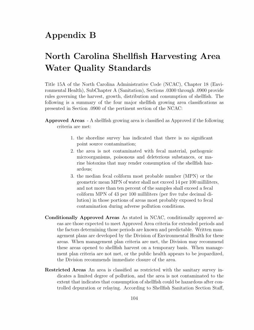
Appendix B
North Carolina Shellfish Harvesting Area
Water Quality Standards
Title 15A of the North Carolina Administrative Code (NCAC), Chapter 18 (Envi-ronmental Health), SubChapter A (Sanitation), Sections .0300 through .0900 providerules governing the harvest, growth, distribution and consumption of shellfish. Thefollowing is a summary of the four major shellfish growing area classifications aspresented in Section .0900 of the pertinent section of the NCAC:
Approved Areas - A shellfish growing area is classified as Approved if the followingcriteria are met:
1. the shoreline survey has indicated that there is no significantpoint source contamination;
2. the area is not contaminated with fecal material, pathogenicmicroorganisms, poisonous and deleterious substances, or ma-rine biotoxins that may render consumption of the shellfish haz-ardous;
3. the median fecal coliform most probable number (MPN) or thegeometric mean MPN of water shall not exceed 14 per 100 milliliters,and not more than ten percent of the samples shall exceed a fecalcoliform MPN of 43 per 100 milliliters (per five tube decimal di-lution) in those portions of areas most probably exposed to fecalcontamination during adverse pollution conditions.
Conditionally Approved Areas As stated in NCAC, conditionally approved ar-eas are those expected to meet Approved Area criteria for extended periods andthe factors determining those periods are known and predictable. Written man-agement plans are developed by the Division of Environmental Health for theseareas. When management plan criteria are met, the Division may recommendthese areas opened to shellfish harvest on a temporary basis. When manage-ment plan criteria are not met, or the public health appears to be jeopardized,the Division recommends immediate closure of the area.
Restricted Areas An area is classified as restricted with the sanitary survey in-dicates a limited degree of pollution, and the area is not contaminated to theextent that indicates that consumption of shellfish could be hazardous after con-trolled depuration or relaying. According to Shellfish Sanitation Section Staff,
104

shellfish may be transported from restricted areas to other areas for cleansingfor a minimum of 14 days.
Prohibited Areas Areas are classified as Prohibited if there is either no currentSanitary Survey, if sanitary survey information indicates that the area does notmeet criteria for an Approved, Conditionally Approved, or Restricted Area.In addition, areas are classified as Prohibited if the growing area is within awastewater treatment plant outfall buffer zone, immediate vicinity of a marina(unless it has less than 30 slips, has no boats over 24 feet in length, or hasno boats with heads or cabins). Specific growing area limits are included inSection .0900 of NCAC.
105

Bibliography
Adam, R. D. (1991). The biology of Giardia spp. Microbiological Reviews 55, 4,706–732.
Alley, W. M. and Smith, P. E. (1981). Estimation of accumulation parameters forurban runoff quality modeling. Water Resources Research 17, 6, 1657–1664.
An, K. H., Lassus, P., Maggi, P., Bardouil, M., and Truquet, P. (1992). Dinoflag-ellate cyst changes and winter environmental-conditions in Vilaine Bay, SouthernBrittany (France). Botanica Marina 35, 1, 61–67.
APHA (2005). Standard methods for the examination of water and wastewater. Amer-ican Public Health Association, Washington, DC, 20th edn.
Arega, F. and Sanders, B. F. (2004). Dispersion model for tidal wetlands. Journalof Hydraulic Engineering-ASCE 130, 8, 739–754.
Ashbolt, N. J., Grohmann, G. S., and Kueh, C. S. W. (1993). Significance of spe-cific bacterial pathogens in the assessment of polluted receiving waters of Sydney,Australia. Water Science and Technology 27, 3/4, 449–452.
Aspinall, L. J. and Kilsby, D. C. (1979). A microbiological quality-control procedurebased on tube counts. Journal of Applied Bacteriology 46, 2, 325–329.
Auer, M. T. and Niehaus, S. L. (1993). Modeling Fecal Coliform Bacteria–I. Fieldand Laboratory Determination of Loss Kinetics. Water Research 27, 4, 693–701.
Badenoch, J., Bartlett, L., Benton, C., Casemore, D., Cawthorne, R., Earnshaw, F.,Ives, K., Jeffery, J., Smith, H., Vaile, M., Warrell, D., and Wright, A. (1990). Cryp-tosporidium in water supplies. Report of the group experts. Tech. rep., Departmentof the Environment, Department of Health. London, UK. HMSO.
Barbe, D. E., Cruise, J. F., and Mo, X. (1996). Modeling the buildup and washoff ofpollutants on urban watersheds. Water Resources Bulletin 32, 3, 511–519.
Bekins, B. A., Godsy, E. M., and Warren, E. (1999). Distribution of microbialphysiologic types in an aquifer contaminated by crude oil. Microbial Ecology 37,4, 263–275.
Beliaeff, B. and Mary, J.-Y. (1993). The most probable number estimate and itsconfidence-limits. Water Research 27, 5, 799–805.
Benham, B. L., Baffaut, C., Zeckoski, R. W., Mankin, K. R., Pachepsky, Y. A.,Sadeghi, A. M., Brannan, K. M., Soupir, M. L., and Habersack, M. J. (2006).Modeling bacteria fate and transport in watersheds to support TMDLs. Transac-tions of the ASABE 49, 4, 987–1002.
106

Bernardo, J. M. and Ramon, J. M. (1998). An introduction to Bayesian referenceanalysis: inference on the ratio of multinomial parameters 47, 1, 101–135.
Berry, D. A. (1996). Statistics: a Bayesian Perspective. Duxbury Press, Belmont,California.
Best, D. J. and Rayner, J. C. W. (1985). A comparison of the MPN and Fisher-Yatesestimators for the density of organisms. Biometrical Journal 27, 2, 167–172.
Beven, K. (2001). How far can we go in distributed hydrological modelling? Hydrologyand Earth System Sciences 5, 1, 1–12.
Bingham, A. K., Jarroll, E. L., and Meyer, E. A. (1979). Giardia-sp - physicalfactors of excystation invitro, and excystation vs eosin exclusion as determinantsof viability. Experimental Parasitology 47, 2, 284–291.
Blanchard, G. F., Sauriau, P. G., Gall, V. C. L., Gouleau, D., Garet, M. J., andOlivier, F. (1997). Kinetics of tidal resuspension of microbiota: Testing the ef-fects of sediment cohesiveness and bioturbation using flume experiments. MarineEcology-Progress Series 151, 17–25.
Bolstad, W. M. (2004). Introduction to Bayesian Statistics. Wiley-Interscience, Hobo-ken, N.J.
Borsuk, M. E., Stow, C. A., and Reckhow, K. H. (2002). Predicting the frequencyof water quality standard violations: A probabilistic approach for TMDL develop-ment. Environmental Science & Technology 36, 10, 2109–2115.
Borsuk, M. E., Stow, C. A., and Reckhow, K. H. (2004). A Bayesian network of eu-trophication models for synthesis, prediction, and uncertainty analysis. EcologicalModelling 173, 2-3, 219–239.
Bowie, G., Mills, W., Porcella, D., Campbell, C., and Chamberlin, C. (1985). Rates,constants, and kinetics formulations in surface water quality modeling. UnitedStates Environmental Protection Agency Office of Research and Development En-vironmental Research Laboratory, Washington, D.C., 2nd edn.
Briones, A. M. and Reichardt, W. (1999). Estimating microbial population countsby ‘most probable number’ using Microsoft Excel R©. Journal of MicrobiologicalMethods 35, 2, 157–161.
Buckalew, D. W., Hartman, L. J., Grimsley, G. A., Martin, A. E., and Register, K. M.(2006). A long-term study comparing membrane filtration with colilert R©definedsubstrates in detecting fecal coliforms and Escherichia coli in natural waters. Jour-nal of Environmental Management 80, 3, 191–197.
107

Cabelli, V. J. (1983). Water-borne Viral Infections In: M. Butler, R. Medlen andR. Morris (eds), “Viruses and Disinfection of Water and Wastewater.”. SurreyPress, Guilford, England.
Cabelli, V. J., Dufour, A. P., McCabe, L. J., and Levin, M. A. (1983). A marine recre-ational water-quality criterion consistent with indicator concepts and risk analysis.Journal Water Pollution Control Federation 55, 10, 1306–1314.
Casella, G. and Berger, R. L. (2002). Statistical Inference. Duxbury, Pacific Grove,California.
Chapra, S. C. (1997). Surface water-quality modeling. Mcgraw-hill series in waterresources and environmental engineering index. McGraw-Hill, New York.
Chapra, S. C., Pelletier, G. J., and Tao, H. (2007). QUAL2K: A modeling frame-work for simulating river and stream water quality, version 2.07: Documentationand user’s manual. Tech. rep., Civil and Environmental Engineering Dept., TuftsUniversity.
Cochran, W. G. (1950). Estimation of bacterial densities by means of the ‘mostprobable number’. Biometrics 6, 2, 105–116.
Cooter, W. S. (2004). Clean water act assessment processes in relation to changingU.S. Environmental Protection Agency management strategies. EnvironmentalScience & Technology 38, 20, 5265–5273.
Davies-Colley, R. J., Bell, R. G., and Donnison, A. M. (1994). Sunlight inactivationof Enterococci and fecal-coliforms in sewage effluent diluted in seawater. Appliedand Environmental Microbiology 60, 6, 2049–2058.
de Man, J. C. (1977). MPN tables for more than one test. European Journal ofApplied Microbiology and Biotechnology 4, 4, 307–316.
Dufour, A. P. and Cabelli, V. J. (1975). Membrane-filter procedure for enumeratingcomponent genera of coliform group in seawater. Applied Microbiology 29, 6, 826–833.
Dufour, A. P., Strickland, E. R., and Cabelli, V. J. (1981). Membrane-filter methodfor enumerating Escherichia coli. Appl. Environ. Microbiol. 41, 5, 1152–1158.
Eckford, R. E. and Fedorak, P. M. (2005). Applying a most probable number methodfor enumerating planktonic, dissimilatory, ammonium-producing, nitrate-reducingbacteria in oil field waters. Canadian Journal of Microbiology 51, 8, 725–729.
Eckner, K. F. (1998). Comparison of membrane filtration and multiple-tube fermen-tation by the colilert and enterolert methods for detection of waterborne coliform
108
bacteria, Escherichia coli, and enterococci used in drinking and bathing water qual-ity monitoring in southern Sweden. Applied and Environmental Microbiology 64,8, 3079–3083.
Eisenhart, C. and Wilson, P. W. (1943). Statistical methods and control in bacteri-ology. Bacteriological Reviews 7, 2, 57–137.
Esham, E. C. and Sizemore, R. K. (1998). Evaluation of two techniques: mFC andmTEC for determining distributions of fecal pollution in small, North Carolinatidal creeks. Water Air and Soil Pollution 106, 1, 179–197.
Fegan, N., Higgs, G., Vanderlinde, P., and Desmarchelier, P. (2004). Enumerationof Escherichia coli O157 in cattle faeces using most probable number techniqueand automated immunomagnetic separation. Letters in Applied Microbiology 38,1, 56–59.
Ferguson, C., Husman, A. M. D., Altavilla, N., Deere, D., and Ashbolt, N. (2003).Fate and transport of surface water pathogens in watersheds. Critical Reviews inEnvironmental Science and Technology 33, 3, 299–361.
Fischer, H. B. (1979). Mixing in inland and coastal waters. Academic Press, NewYork.
Food and Drug Administration and Interstate Shellfish Sanitation Conference (2005).National Shellfish Sanitation Program - guide for the control of molluscan shellfish.
Gameson, A. and Gould, D. (1974). Effects of solar radiation on the mortality ofsome terrestrial bacteria in sea water. In International Symposium on Dischargeof Sewage from Sea Outfalls, vol. Paper No. 22, London. Pergamon Press.
Garthright, W. E. (1993). Bias in the logarithm of microbial density estimates fromserial dilutions. Biometrical Journal 35, 3, 299–314.
Garthright, W. E. (1997). A Bayesian analysis of serial dilutions offers a worsepositive bias than the MPN and proposes an inappropriate interval estimate. FoodMicrobiology 14, 5, 515–517.
Gelman, A. (2006). Prior distributions for variance parameters in hierarchical models(comment on article by Browne and Draper). Bayesian Analysis 1, 3, 515–534.
Ghinsberg, R. C., Dov, L. B., Sheinberg, Y., Nitzan, Y., and Rogol, M. (1994).Monitoring of selected bacteria and fungi in sand and sea-water along the Tel-avivcoast. Microbios 77, 310, 29–40.
Grant, S. B., Sanders, B. F., Boehm, A. B., Redman, J. A., Kim, J. H., Mrse, R. D.,Chu, A. K., Gouldin, M., McGee, C. D., Gardiner, N. A., Jones, B. H., Svejkovsky,
109
J., and Leipzig, G. V. (2001). Generation of Enterococci bacteria in a coastalsaltwater marsh and its impact on surf zone water quality. Environmental Science& Technology 35, 12, 2407–2416.
Greenwood, M. and Yule, G. U. (1917). On the statistical interpretation of somebacteriological methods employed in water analysis. The Journal of Hygiene 16,1, 36–54.
Gronewold, A. D., Borsuk, M. E., Wolpert, R. L., and Reckhow, K. H. (2008). An as-sessment of fecal indicator bacteria-based water quality standards. EnvironmentalScience & Technology 42, 13, 4676–4682.
Gronewold, A. D. and Reckhow, K. H. (2007). Developing a Bayesian network modelfor bacteriologically impaired surface waters. In proceedings of the 7th Interna-tional (IWA) Symposium on Systems Analysis and Integrated Assessment in WaterManagement (Washington, D.C., USA).
Gronewold, A. D. and Wolpert, R. L. (2008). Modeling the relationship betweenmost probable number (MPN) and colony-forming unit (CFU) estimates of fecalcoliform concentration. Water Research 42, 13, 3327–3334.
Gronewold, A. D., Wolpert, R. L., Noble, R. T., Coulliette, A. D., and Reckhow,K. H. (2007). Developing a Bayesian network model for supporting fecal coliformTMDL assessments. In proceedings of the Water Environment Federation SpecialtyConference - TMDL 2007 (Bellevue, Washington, USA).
Hackney, C. R. and Pierson, M. D. (1994). Environmental indicators and shellfishsafety. Chapman & Hall, New York.
Harris, A. S. D., Jones, K. J., and Lewis, J. (1998). An assessment of the accuracyand reproducibility of the most probable number (MPN) technique in estimatingnumbers of nutrient stressed diatoms in sediment samples. Journal of ExperimentalMarine Biology and Ecology 231, 1, 21–30.
Horowitz, A. (1986). Comparison of methods for the concentration of suspendedsediment in river water for subsequent chemical analysis. Environmental Science& Technology 20, 2, 155–160.
Houck, O. A. (2002). The Clean Water Act TMDL program: law, policy, and imple-mentation. Environmental Law Institute, Washington, D.C., 2nd edn.
Hurley, M. A. and Roscoe, M. E. (1983). Automated statistical analysis of microbialenumeration by dilution series. Journal of Applied Bacteriology 55, 1, 159–164.
Irvine, K. N. and Pettibone, G. W. (1993). Dynamics of indicator bacteria popula-tions in sediment and river water near a combined sewer outfall. EnvironmentalTechnology 14, 6, 531–542.
110

Jakeman, A. J. and Letcher, R. A. (2003). Integrated assessment and modelling: Fea-tures, principles and examples for catchment management. Environmental Mod-elling & Software 18, 6, 491–501.
Jeffreys, H. (1946). An invariant form for the prior probability in estimation problems.Proceedings of the Royal Society of London Series A– Mathematical and PhysicalSciences 186, 1007, 453–461.
Jensen, F. V., Olesen, K. G., and Andersen, S. K. (1990). An algebra of Bayesianbelief universes for knowledge-based systems. Networks 20, 5, 637–659.
Johnson, D. C., Enriquez, C. E., Pepper, I. L., Davis, T. L., Gerba, C. P., and Rose,J. B. (1997). Survival of Giardia, Cryptosporidium, poliovirus and salmonella inmarine waters. Water Science and Technology 35, 11-12, 261–268.
Kashefipour, S. M., Lin, B., and Falconer, R. A. (2005). Neural networks for pre-dicting seawater bacterial levels. Proceedings of The Institution of Civil Engineers-Water Management 158, 3, 111–118.
Ketchum, B. (1951). The exchanges of fresh and salt waters in tidal estuaries. Journalof Marine Research 10, 1, 18–38.
Kinzelman, J., Ng, C., Jackson, E., Gradus, S., and Bagley, R. (2003). Entero-cocci as indicators of Lake Michigan recreational water quality: Comparison oftwo methodologies and their impacts on public health regulatory events. Appliedand Environmental Microbiology 69, 1, 92–96.
Klee, A. J. (1993). A computer-program for the determination of most probablenumber and its confidence-limits. Journal of Microbiological Methods 18, 2, 91–98.
Kloot, R. W., Radakovich, B., Huang, X.-Q., and Brantley, D. (2006). A compar-ison of bacterial indicators and methods in rural surface waters. EnvironmentalMonitoring and Assessment 121, 1, 275–287.
Kuo, A. and Neilson, B. (1988). Modified Tidal Prism Model for Water Quality inSmall Coastal Embayments. Water Science and Technology 20, 6/7, 133–142.
Kuo, A., Park, K., Kim, S., and Lin, J. (2005). A Tidal Prism Water Quality Modelfor Small Coastal Basins. Coastal Management 33, 1, 101–117.
Larrazabal, M. E., Lassus, P., Maggi, P., and Bardouil, M. (1990). Modern dinoflag-ellate kysts in Vilaine Bay Southern Brittany (France). Cryptogamie Algologie 11,3, 171–185.
LeClerc, H., Mossel, D. A. A., Edberg, S. C., and Struijk, C. B. (2001). Advancesin the bacteriology of the coliform group: Their suitability as markers of microbialwater safety. Annual Review of Microbiology 55, 201–234.
111

Lee, J. H. and Bang, K. W. (2000). Characterization of urban stormwater runoff.Water Research 34, 6, 1773–1780.
Levin, M. A., Fischer, J. R., and Cabelli, V. J. (1975). Membrane filter technique forenumeration of enterococci in marine waters. Applied Microbiology 30, 1, 66–71.
Luketina, D. (1998). Simple Tidal Prism Models Revisited. Estuarine, Coastal andShelf Science 46, 1, 77–84.
Lunn, D. J., Thomas, A., Best, N., and Spiegelhalter, D. (2000). WinBUGS-ABayesian modelling framework: Concepts, structure, and extensibility. Statisticsand Computing 10, 4, 325–337.
Mancini, J. L. (1978). Numerical estimates of coliform mortality-rates under variousconditions. Journal Water Pollution Control Federation 50, 11, 2477–2484.
McBride, G. B. (2003). Preparing exact most probable number (mpn) tables usingoccupancy theory, and accompanying measures of uncertainty. NIWA TechnicalReport 121 62.
McBride, G. B. (2005). Using statistical methods for water quality management.Issues, problems and solutions. John Wiley & Sons Ltd Chichester, UK.
McBride, G. B., McWhirter, J. L., and Dalgety, M. H. (2003). Uncertainty in mostprobable number calculations for microbiological assays. Journal of AOAC Inter-national 86, 5, 1084–1088.
McCrady, M. H. (1915). The numerical interpretation of fermentation tube results.Journal of Infectious Diseases 17, 1, 183–212.
McMurry, S. W., Coyne, M. S., and Perfect, E. (1998). Fecal coliform transportthrough intact soil blocks amended with poultry manure. Journal of EnvironmentalQuality 27, 1, 86–92.
Medema, G. J., Bahar, M., and Schets, F. M. (1997). Survival of Cryptosporid-ium parvum, Escherichia coli, faecal Enterococci and Clostridium perfringens inriver water: Influence of temperature and autochthonous microorganisms. WaterScience and Technology 35, 11, 249–252.
Menyah, M. K. and Sato, K. (1996). A proposal for re-evaluating the most probablenumber procedure for estimating numbers of Bradyrhizobium spp. Biology andFertility of Soils 23, 2, 110–112.
Mitchell, R. and Chamberlin, C. (1979). Indicators of viruses in water and food(edited by Berg G.). 1–12. Ann Arbor Science Publishers, Inc, Ann Arbor, MI.
112

Moeller, J. R. and Calkins, J. (1980). Bactericidal agents in waste-water lagoons andlagoon design. Journal Water Pollution Control Federation 52, 10, 2442–2451.
National Research Council (2001). Assessing the TMDL approach to water qualitymanagement.
N.C. Department of Environment and Natural Resources (2004). Coastal recreationalwaters monitoring, evaluation, and notification rules: 15a ncac 18a .3400.
NCDENR (2007). Study on comparison between CFU and MPN estimates of fecalcoliform concentration.
Neumann, C. M., Harding, A. K., and Sherman, J. M. (2006). Oregon Beach mon-itoring program: Bacterial exceedances in marine and freshwater creeks/outfallsamples, October 2002-April 2005. Marine Pollution Bulletin 52, 10, 1270–1277.
Nix, P. G., Daykin, M. M., and Vilkas, K. L. (1993). Sediment bags as an integratorof fecal contamination in aquatic systems. Water Research 27, 10, 1569–1576.
Noble, R. T. and Fuhrman, J. A. (1997). Virus decay and its causes in coastal waters.Applied and Environmental Microbiology 63, 1, 77–83.
Noble, R. T., Moore, D. F., Leecaster, M. K., McGee, C. D., and Seisberg, S. B.(2003a). Comparison of total coliform, fecal coliform, and enterococcus bacterialindicator response for ocean recreational water quality testing. Water Research37, 7, 1637–1643.
Noble, R. T., Seisberg, S. B., Leecaster, M. K., McGee, C. D., Ritter, K. J., Walker,K. O., and Vainik, P. M. (2003b). Comparison of beach bacterial water qualityindicator measurement methods. Environmental Monitoring and Assessment 81,1, 301–312.
Novotny, V. and Olem, H. (1994). Water quality: Prevention, identification, andmanagement of diffuse pollution. Van Nostrand Reinhold, New York, 1st edn.
Obiri-Danso, K. and Jones, K. (2000). Intertidal sediments as reservoirs for hip-purate negative Campylobacters, Salmonellae and faecal indicators in three E.U.recognised bathing waters in northwest England. Water Research 34, 2, 519–527.
Ott, W. (1995). Environmental statistics and data analysis. Lewis Publishers, BocaRaton.
Papen, H. and von Berg, R. (1998). A most probable number method (MPN) for theestimation of cell numbers of heterotrophic nitrifying bacteria in soil. Plant andSoil 199, 1, 123–130.
113

Pearl, J. (1988). Probabilistic reasoning in intelligent systems: Networks of plausibleinference. Morgan Kaufmann Publishers, San Mateo, Calif.
Qian, S. S., Donnelly, M., Schmelling, D. C., Messner, M., Linden, K. G., and Cotton,C. (2004). Ultraviolet light inactivation of protozoa in drinking water: a Bayesianmeta-analysis. Water Research 38, 2, 317–326.
Qian, S. S., Linden, K. G., and Donnelly, M. (2005). A Bayesian analysis of mouseinfectivity data to evaluate the effectiveness of using ultraviolet light as a drinkingwater disinfectant. Water Research 39, 17, 4229–4239.
R Development Core Team (2006). R: A Language and Environment for StatisticalComputing. R Foundation for Statistical Computing, Vienna, Austria. ISBN 3-900051-07-0.
Reckhow, K. H. (1994). Water-quality simulation modeling and uncertainty analysisfor risk assessment and decision-making. Ecological Modelling 72, 1, 1–20.
Reckhow, K. H. (1999). Water quality prediction and probability network models.Canadian Journal of Fisheries and Aquatic Sciences 56, 7, 1150–1158.
Reeves, R. L., Grant, S. B., Mrse, R. D., Oancea, C. M. C., Sanders, B. F., andBoehm, A. B. (2004). Scaling and management of fecal indicator bacteria in runofffrom a coastal urban watershed in southern california. Environmental Science &Technology 38, 9, 2637–2648.
Rippey, S. R., Adams, W. N., and Watkins, W. D. (1987). Enumeration of fecal-coliforms and Escherichia-coli in marine and estuarine waters - an alternative tothe APHA-MPN approach. Journal Water Pollution Control Federation 59, 8,795–798.
Rompre, A., Servais, P., Baudart, J., de Roubin, M.-R., and Laurent, P. (2002).Detection and enumeration of coliforms in drinking water: current methods andemerging approaches. Journal of Microbiological Methods 49, 1, 31–54.
Rose, R. E., Geldreich, E. E., and Litsky, W. (1975). Improved membrane-filtermethod for fecal coliform analysis. Applied Microbiology 29, 4, 532–536.
Roussanov, B., Hawkins, D. M., and Tatini, S. R. (1996). Estimating bacterial densityfrom tube dilution data by a Bayesian method. Food Microbiology 13, 5, 341–363.
Russek, E. and Colwell, R. R. (1983). Computation of most probable numbers. Appl.Environ. Microbiol. 45, 5, 1646–1650.
Salomon, J. C. and Pommepuy, M. (1990). Mathematical-model of bacterial-contamination of the morlaix estuary (france). Water Research 24, 8, 983–994.
114

Sanders, B. F., Arega, F., and Sutula, M. (2005). Modeling the dry-weather tidalcycling of fecal indicator bacteria in surface waters of an intertidal wetland. WaterResearch 39, 14, 3394–3408.
Sanford, L., Boicourt, W., and Rives, S. (1992). Model for estimating tidal flushingof small embayments. Journal of Waterway, Port, Coastal and Ocean Engineering118, 6, 635–654.
Sayler, G. S., Nelson, J. D., Justice, A., and Colwell, R. R. (1975). Distributionand significance of fecal indicator organisms in Upper Chesapeake Bay. AppliedMicrobiology 30, 4, 625–638.
Schijven, J. F. and Hassanizadeh, S. M. (2000). Removal of viruses by soil passage:Overview of modeling, processes, and parameters. Critical Reviews In Environ-mental Science and Technology 30, 1, 49–127.
Schijven, J. F. and Hassanizadeh, S. M. (2002). Virus removal by soil passage at fieldscale and groundwater protection of sandy aquifers. Water Science and Technology46, 3, 123–129.
Schmee, J. and Hahn, G. J. (1979). A simple method for regression analysis withcensored data. Technometrics 21, 4, 417–432.
Shen, J., Sun, S.-C., and Wang, T.-P. (2005). Development of the fecal coliform totalmaximum daily load using Loading Simulation Program C++ and tidal prismmodel in estuarine shellfish growing areas: A case study in the Nassawadox coastalembayment, Virginia. J. Environ. Sci. Heal. A 40, 9, 1791–1807.
Smith, E. P., Ye, K. Y., Hughes, C., and Shabman, L. A. (2001). Statistical assess-ment of violations of water quality standards under section 303(d) of the CleanWater Act. Environmental Science & Technology 35, 3, 606–612.
Spiegelhalter, D., Dawid, A., Lauritzen, S., and Cowell, R. (1993). Bayesian Analysisin Expert Systems. Statistical Science 8, 3, 219–247.
Spiegelhalter, D. J., Thomas, A., Best, N. G., and Lunn, D. J. (2003). WinBUGSversion 1.4 user manual. Tech. rep., Medical Res. Counc. Biostat. Unit, Cambridge,UK.
Tanner, M. A. (1991). Tools for Statistical Inference. Springer-Verlab, New York,NY.
Thomann, R. V. and Mueller, J. A. (1987). Principles of surface water quality mod-eling and control. Harper & Row, New York.
Thomas, G. W. and Phillips, R. E. (1979). Consequences of water-movement inmacropores. Journal of Environmental Quality 8, 2, 149–152.
115

Tillett, H. E. and Coleman, R. (1985). Estimated numbers of bacteria in samplesfrom non-homogeneous bodies of water - how should mpn and membrane filtrationresults be reported. Journal of Applied Bacteriology 59, 4, 381–388.
Tzipori, S. (1983). Cryptosporidiosis in animals and humans. Microbiological Reviews47, 1, 84–96.
U.S. Environmental Protection Agency (2001). Protocol for developing pathogenTMDLs. Tech. Rep. EPA 841-R-00-002, Office of Water (4503F), United StatesEnvironmental Protection Agency, Washington, DC.
U.S. Environmental Protection Agency (2002). National water quality inventory:Report to congress (2002 reporting cycle), EPA 841-R-07-001.
U.S. Environmental Protection Agency (2005a). Code of federal regulations: Title40, chapter 1, part 141.
U.S. Environmental Protection Agency (2005b). Guidance for 2006 assessment, listingand reporting requirements pursuant to sections 303(d), 305(b) and 314 of theClean Water Act.
U.S. Geological Survey (1996). Water quality of the Lower Columbia River Basin:Analysis of current and historical water-quality data through 1994 (Water-resources investigations report 95-4294), 52-53. Tech. rep., U.S. Geological Survey.
Vandenberghe, V., Bauwens, W., and Vanrolleghem, P. A. (2007). Evaluation ofuncertainty propagation into river water quality predictions to guide future moni-toring campaigns. Environmental Modelling & Software 22, 5, 725–732.
Weisberg, S. (2005). Applied linear regression. Wiley series in probability and statis-tics. Wiley-Interscience, Hoboken, N.J., 3rd edn.
Weiskel, P. K., Howes, B. L., and Heufelder, G. R. (1996). Coliform contaminationof a coastal embayment: Sources and transport pathways. Environmental Science& Technology 30, 6, 1872–1881.
White, N. M., Line, D. E., Potts, J. D., Kirby-Smith, W., Doll, B., and Hunt, W. F.(2000). Jump Run Creek shellfish restoration project. Journal of Shellfish Research19, 1, 473–476.
Woodward, R. L. (1957). How probable is the most probable number? Journal ofthe American Water Works Association 49, 1, 1060–1068.
Woomer, P. L., Bennett, J., and Yost, R. (1990). Overcoming the inflexibility ofmost-probable-number procedures. Agronomy Journal 82, 2, 349–353.
116

Biography
My research and career objectives first took shape during my undergraduate educa-
tion at Cornell University’s School of Civil and Environmental Engineering. After
graduating from Cornell in 1995, I was employed as a project manager and licensed
professional engineer with the environmental engineering consulting firms Stearns &
Wheler, LLC and the Ecological Engineering Group, Inc. Between 1995 and 2003
I initiated and completed over forty planning, design, and construction projects in
areas of wastewater, water, and solid waste management. Significant project accom-
plishments include obtaining grant funding for point and non-point source pollution
mitigation projects in small communities through the Massachusetts Coastal Zone
Management (CZM) Coastal Pollutant Remediation (CPR) program, and serving as
the resident engineering during the closure of a 54-acre municipal solid waste landfill.
I also completed a series of comprehensive watershed and wastewater management
planning studies for rapidly growing communities in southeastern Massachusetts.
Each planning project included a detailed analysis of environmental management
infrastructure alternatives, evaluation of public policy and regulatory issues, and ex-
tensive field work to determine hydrogeological and surface water quality conditions.
In addition to my work as an environmental engineer, I began supervising and
coordinating a wide variety of research projects in 1999 as a scientist and teacher
with the Sea Education Association (SEA) based in Woods Hole, Massachusetts. I
have since logged over 200 days at sea as a teacher with SEA while advising high
117

school and college-level students during the data gathering and report writing phases
of individual research projects, including non-point source pollution analysis of nu-
trient loading in Samana Bay in the Dominican Republic and distribution of spiny
lobster larvae across the gulf stream. As a student with SEA, I investigated the
impacts of stormwater runoff on eutrophication in St. George’s Harbor, Bermuda,
and subsequent implications for outbreak of shellfish-borne diseases such as paralytic
shellfish poisoning (PSP) and ciguatera. My experience with SEA provided a unique
perspective on global environmental problems through coastal research projects in
Nova Scotia, Bermuda, the Lesser Antilles, and Central America. My passion for
teaching, research, and pursuing graduate study was confirmed by my experience
with SEA, and my enthusiasm persisted through adverse conditions at sea such as
severe weather, sleep deprivation, and seasickness. Throughout my experiences in
engineering consulting and with SEA, however, I repeatedly questioned traditional
approaches to addressing uncertainty in water quality measurements, construction
cost estimates, and other critical environmental management decision criteria. These
questions inspired my return to graduate school and my work on Bayesian statistical
models.
I began graduate studies at the Nicholas School of the Environment at Duke Uni-
versity under the guidance of Drs. Kenneth H. Reckhow and Robert L. Wolpert.
My research focused on applying statistical models to help solve environmental re-
source and infrastructure management problems. I specialize in developing innovative
118

modeling tools which integrate monitoring data from multiple spatial and temporal
scales to characterize interrelated meteorological and hydrological processes, as well
as ecosystem response dynamics. My doctorate research focuses on developing mod-
eling tools for evaluating climate change, land use, and pollutant mitigation scenarios
to restore water quality in impaired shellfish harvesting waters in Eastern North Car-
olina. Significant contributions from this research include a new set of water quality
standards imposing limits on parameters of the true fecal bacteria concentration
(the applicable measure of water quality), as opposed to traditional standards which
impose limits on most probable number (MPN) and colony-forming unit (CFU) con-
centration point estimates. This research recently appeared as a cover article in En-
vironmental Science & Technology. I also developed an innovative approach to mod-
eling the relationship between alternative measures of fecal coliform concentration,
which provided important guidance to shellfish harvesting area managers currently
debating a shift in standard laboratory protocol. This research recently appeared
in Water Research. The contributions of my graduate work to the scientific com-
munity were acknowledged through several awards and scholarships, including the
Water Environment Federation Robert Canham Graduate Scholarship, the North
Carolina Association of Environmental Professionals Graduate Scholarship, and the
QEA, LLC Graduate Scholarship. In addition, I received an Outstanding Student
Paper Award for a presentation of my research at the American Geophysical Union
(AGU) Fall 2007 Meeting.
119

While conducting my research at Duke, I also served as the primary instructor
for the Nicholas School of the Environment graduate-level course in water quality
management, and periodically served as a guest lecturer for courses in water quality
modeling and probability. I consistently received positive evaluations from students
at Duke and at SEA, and was awarded the Nicholas School of the Environment
teaching assistant of the year award after my first year of graduate study.
120


![DemographicPredictorsofPeanut,TreeNut,Fish, Shellfish ...downloads.hindawi.com/archive/2012/858306.pdf · tree nut and shellfish allergy less common in males [12, 15– 18]. However,](https://img.pdfslide.net/doc/110x75/5f6ec31a8603e75b967f5f72/demographicpredictorsofpeanuttreenutfish-shellish-tree-nut-and-shellish.jpg)