Embed Size (px)
Citation preview

DEPARTMENT OF CIVIL ENGINEERING
Water Resources Research Group
Software ProfileA User Manual for QUANTARE
m m
UNIVtraiY D epartm ent o f C ivil Engineering, University o f Salford, Sa lfo rd , M5 4WT, bSALPORD U.K. Telephone: 061-736 5843. Telex: 68741 (Salcel). Fax: 061-745 7027.
fvj (kfc Ayuj I ! a n
QUANTARE(Quantitative Areal Rainfall Estimation)
A program for displaying spatial rainfall and computing areal rainfall totals for pre-defined catchments from point
raingauge rainfall data, utilising two-dimensional interpolation algorithms.
Software ProfileA User Manual for QUANTARE
June 1991
ENVIRONMENT AGENCY
Water Resources Research Group Department of Civil Engineering
University of Salford Salford
M5 4WT
Report Prepared by
1CA. Tilford June 1991
Contents
List of Figures
1. Introduction
2 . Typography and Flow C hart Symbols
3 . Software Specification and System Requirements
4 . Areal Rainfall Estimation4.1. Spatial Rainfall Fields and Catchment Totals from Sparse Raingauge Data4.2. TWo-Dimensional Interpolation
4.2.1. Renka and Cline Method4.2.2. Modified Shepherd Method
4.3. Other Information
5 . Program Structure and Data Requirements5.1. StructureS .2. Input and Output Datafiles5.3. Include File5.4. Presentation of Results
6 . Running the Program6.1. Device Type6.2. Options Menu6.3. Adjustment Date6.4. Rainfall Scale Slicing6.5. Linking QUANTARE (Auxiliary Code)6.6. Running’QUANTARE6.7. Example Run-Time Session
7 . Customised Implementation of QUANTARE
8 . C onclusions
Bibliography
AppendicesAppendix 1 Source Code ListingAppendix 2 Include FiteAppendix 3 Example Raingauge Rainfall InputfileAppendix 4 Example Catchment InputfileAppendix 5 Example OutputfileAppendix 6 Runtime ListingAppendix 7 Devices SupportedAppendix 8 Utility Program Source Listing (set Jdom)

List o f Figures
Figure 1. Schematic representation of the display of spatial rainfall patterns and thecomputation of catchment areal totals
Figure 2. Interpolation Domain (Northern Area, National Rivers Authority, Anglian Region)Figure 3. Program Flowchart Figure 4. Example Rainfall Datafile Figure 5. Sub-Region and Interpolation Domain

page 1
1. Introduction
This manual is a report in a series of Technical Reports produced by the Water Resources Research Group at the
Department of Civil Engineering, University of Salford.
The manual is a reference to the software package known as QUANTARE (Quantitative Areal Rainfall Estimation), a program for displaying spatial rainfall fields and computing quantitative areal rainfall totals for pre-defined catchments, from point raingauge rainfall data. The report begins by stating the software specification and goes on to discuss the input files required. The structure of QUANTARE is described and illustrated with a flowchart and an example run-time session described. Annotated samples of the input datafiles are included. Whilst the report concentrates on a single example (National Rivers Authority, Anglian Region, Northern Area), QUANTARE has been designed and structured so that customisation and implementation in other areas is straightforward and a chapter is dedicated to this.
The Appendices provide a source listing of the program together with hard copy listings of example input and
output datafiles. The datafiles accompany the program on the distribution disk and may be used to replicate the run-time example in the report main body. User input datafiles should exactly replicate the format of the
example datafiles.
This manual is not a definitive guide to the interpolation routines used. Further information can be found in the references listed in the bibliography.
The Water Resources Research Group would welcome any comments on this Software Profile. Please contact Professor lan Cluckie at the address on the front of the repent

page 2
2 . Typography and Flow Chart Symbols
The body of this manual is printed in a nonnal (Times font) typeface; other typefaces have special meanings.
Courier is used for the listings of the program, datafiles and screen output. B o ld e d c o u r i e r represents interactive user keyboard input whilst annotated comments of source code and datafile listings are made in bolded times.
The program structure is illustrated by a flowchart and described (summarised) textually. Algorithms are described in terms of steps such as input, output and computations. Decisions are made by testing Boolean expressions that are evaluated to be true or false. The flowchart symbols for these processes, along with a
symbol to indicate beginning and end are:
Assignments or computations
Input or output
Boolean expressions
Start or stop

page 3
3. Software Specification and System Requirements
QUANTARE is an interactive, graphically based FORTRAN program. The software is coded in ANSI FORTRAN 77 and has been developed on a Digital Electronic Company (DEC) Micro VAX n minicomputer using VMS v5.4 and VAX FORTRAN 77 v5.5. The code utilises some VAX FORTRAN 77 implementations (extensions) and this should be considered before attempting to port the code to a different environment
The two-dimensional interpolation and surface fitting algorithms are part of the Numerical Algorithms Group (Mark 14) Fortran Library1.
Graphics play an integral role in the presentation of results in QUANTARE and are facilitated by UNIRAS Graphics Software1 package (Version 6.0). UNIRAS graphics modules are upwardly compatible with subsequent releases of UNIRAS. UNIRAS graphics modules are machine independent and can be implemented on a wide range of machines. A menu of devices for which the graphics elements of the software have already been implemented prompt the user to indicate the device on which the software is running enabling the correct device driver to be software selected. Implementation for new devices is straightforward if a UNIRAS driver for the device is available. It is envisaged that incorporation of an alternative graphics package (capable of producing two-dimensional colour or black-and-white surface plots) into QUANTARE would be straightforward.
1 Numerical Algorithms Group Lid, Wilkinson House, Jordan Hill Road, Oxford, 0X 2 8DR, UNITED KINGDOMNAG Inc, 1400 Opus Place, Suite 200, Downers Grove, IL 60515-5702, USA.
3 UNIRAS A.S.,376 Gladsaxevej, DK-2860 Sflborg. DENMARKUNIRAS Lid, Ambassador House, 181 Famham Road, Slough, SL1 4XP, UNITED KINGDOM.

page 4
4. Areal Rainfall Estimation
tybter resource management usually requires estimates of areal rainfall rather than point rainfall estimates. In
particular, an accurate assessment of areal rainfall is a necessary basic input to rainfall-runoff models (perhaps the most substantial user of real-time rainfall data), especially conceptual models which utilise a water balance approach. Numerous methods of determining areal rainfall from point raingauge measurements have been proposed (e.g. see the review conducted by Hall and Barclay, 1975, and the objective comparisons of Creutin and Obled, 1982) and the techniques proposed vary greatly in terms of complexity, from the simplest deterministic methods, (e.g. nearest neighbour method, arithmetic mean, Thiessen, subjective isohyetal) to the more sophisticated stochastic methods such as bicubic-spline surfaces, optimal interpolation, and kriging.
The report is not judgmental and does not state the accuracy, reliability, shortcomings or advantages of one interpolation technique over another, or any other procedure over interpolation.
4 .1 . Spatial Rainfall Fields and Catchment Totals from Sparse Raingauge Data
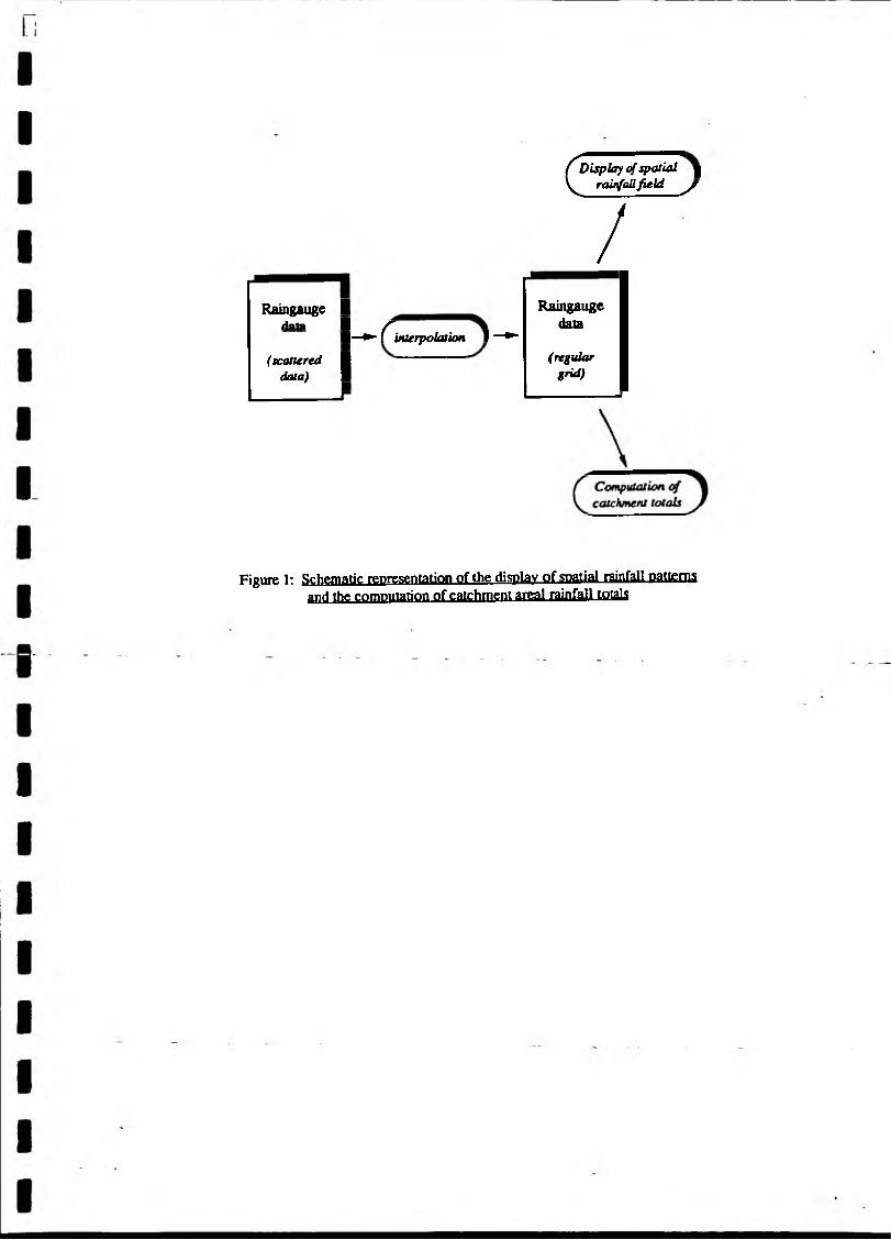
QUANTARE derives a representation of the spatial rainfall field and estimates areal rainfall depths over predefined catchments. This is achieved by interpolating irregularly distributed point raingauge rainfall depths to
a (5 km) regular grid, the grid nodes being used to construct the spatial rainfall field and to compute catchment rainfall.
Each phase in the process is shown schematically in figure 1.
4 .2 . Two-Dimensional Interpolation
This section introduces the two-dimensional interpolation algorithms supported by QUANTARE. The algorithms work with irregularly distributed data (although many solutions to related problems in two- dimensional interpolation have been in long use, interpolation functions making an exact fit for irregularly spaced data are rare [when the data points are on a regular grid, many solutions are possible]). The choice
regarding the interpolation algorithm used by QUANTARE is made by the user at run-time.
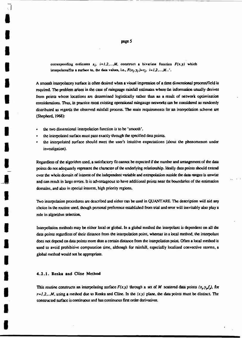
The fundamental problem that any interpolation procedure for two-dimensional data scattered in the plane addresses is the following (after Renka and Cline, 1984):
‘...given a set of nodes (abscissae) arbitrarily distributed in the x-y plane, with
page 5
corresponding ordinates Zj, i=l construct a bivariate function F(x,y) whichmteipolales/fits a surface to, the data values, i.e., F (x^yi,)= 2 ,̂
A smooth interpolatory surface is often desired when a visual impression of a three dimensional proces^field is required. The problem arises in the case of raingauge rainfall estimates where the information usually derives
from points whose locations are determined logistically rather than as a result of network optimisation considerations. Thus, in practice most existing operational raingauge networks can be considered as randomly distributed as regards the observed rainfall process. The main requirements for an interpolation scheme are (Shepherd, 1968):
• the two dimensional interpolation function is to be ‘smooth*.• the interpolated surface must pass exactly through the specified data points.• the interpolated surface should meet the user's intuitive expectations (about the phenomenon under
investigation).
Regardless of the algorithm used, a satisfactory fit cannot be expected if the number and arrangement of the data points do not adequately represent the character of the underlying relationship. Ideally data points should extend over the whole domain of interest of the independent variable and extrapolation outside the data ranges is unwise and can result in large errors. It-is advantageous to have additional points near the boundaries of the estimation domains, and also in special interest, high priority regions.
Two interpolation procedures are described and either can be used in QUANTARE. The description will aid any choice in the routine used, though personal preference established from trial and error will inevitably also play a
role in algorithm selection.
Interpolation methods may be either local or global. In a global method the interpolant is dependent on all the data points regardless of their distance from the interpolation point, whereas in a local method, the interpolant
does not depend on data points more than a certain distance from the interpolation point Often a local method is used to avoid prohibitive computation time, although for rainfall, especially localised convective storms, a
global method would not be appropriate.
4 .2 .1 . Renka and Cline Method
This routine constructs an interpolating surface F(x,y) through a set of M scattered data points forr = l using a method due to Renka and Cline. In the (x,y) plane, the data points must be distinct The constructed surface is continuous and has continuous first order derivatives.
page 6
The method involves firstly creating a triangulation with all the (x.y) data points as nodes, the triangulation being as nearly equi-angular as possible (Cline and Renka, 1984). Then gradients in the x- and y-directions are estimated at node r, for r=l as the partial derivatives of a quadratic function of x and y whichinterpolates the data value f r and which fits the data values at nearby nodes (those within a certain distance chosen by the algorithm) in a weighted least square sense. The weights are chosen such that closer nodes have
more influence than more distant nodes on derivative estimates at node r. The computed partial derivatives, with the f r values, at the three nodes of each triangle define a piecewise polynomial surface of certain form which is the interpolant on that triangle. More detailed information on the algorithm is provided in Renka and Cline (1984), Lawson (1977), and Renka (1984).
The interpolant F(x,y) can be subsequently evaluated at any point (x,y) inside or outside the domain of the data in the second stage routine (see below). Points outside the domain of the data are determined by extrapolation.
The second stage routine computes the interpolant for a specified grid. The routine takes as input the parameters defining the interpolant F(x,y) of a set of scattered data points (xr yr/r), for r -1 2 ,~.Mt and evaluates the interpolant at the point (pxj>y). If (pxjyy) is equal to (*r yr) for some value of r, the returned value will be equal to Jr. If (pxjjy) is not equal to (xryP) for any r, the derivatives passed to the routine are used to compute the inteipolant A triangle is sought which contains the point (pxpy), and the vertices of the triangle along with the partial derivatives and f r values at the-vertices are used to compute the value F(pxj)y). If the”point (pxjpy) lies outside the triangulation defined by the input parameters, the returned value is obtained by extrapolation. In this case, the interpolating function F is extended linearly beyond the triangulation boundary.
4 .2 .2 . Modified Shepherd Method
This routine constructs an interpolating surface F(x,y) through a set of M scattered data points (xryrf f), for r= l,2,..M , using a modification of Shepherd's method. The surface is continuous and has continuous first
derivatives.
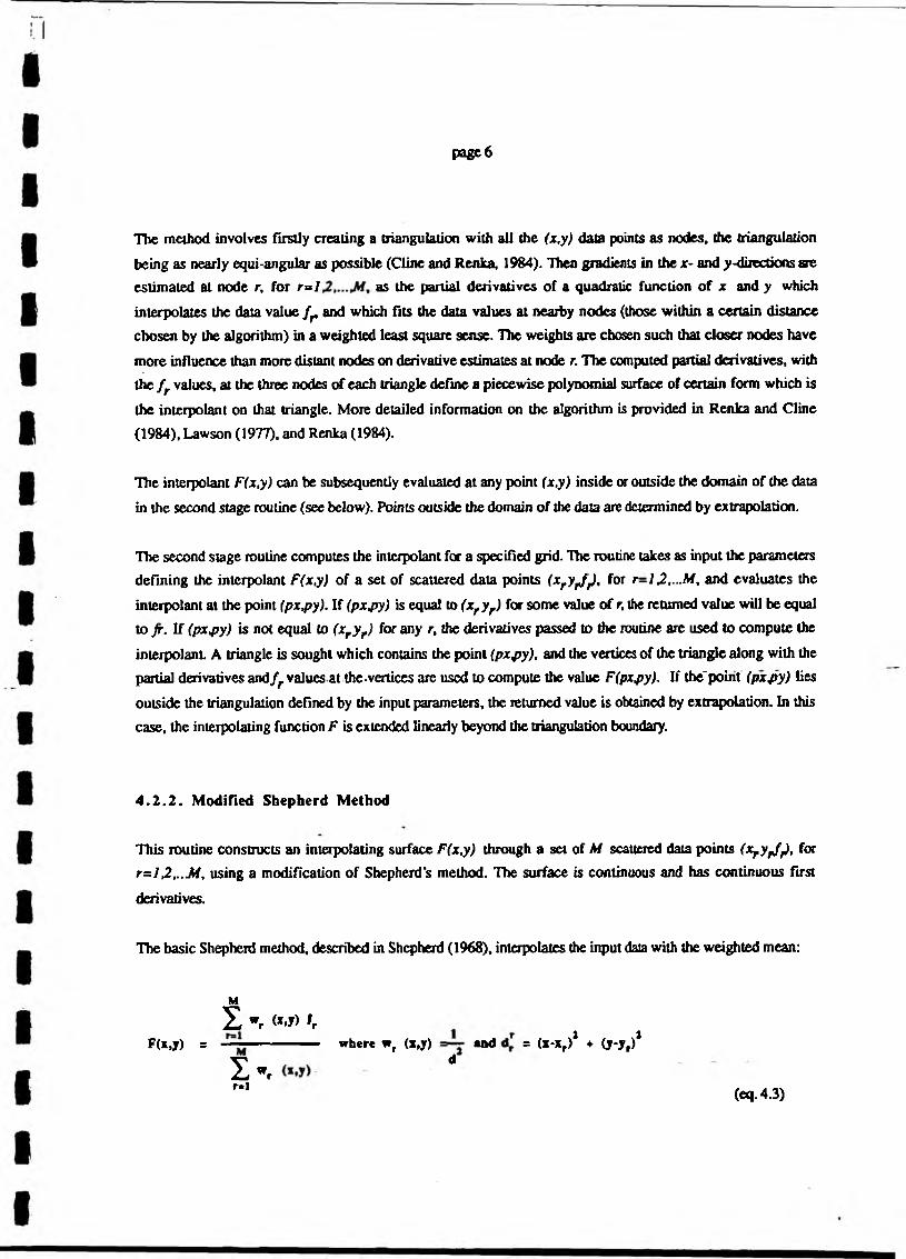
The basic Shepherd method, described in Shepherd (1968), interpolates the input data with the weighted mean:
M
X Wr (x>f) frF(x,y) = --------------- where wf (x,y) and = (x-xr)2 + (y-yr)2
X Wr d
^ (eq. 4.3)

page 7
The basic method is global in that the interpolated value at any point depends on all the data, but the method uses a modification due to Franke and Neil son (1980), whereby the method becomes local by adjusting each *>/x,y) to be zero outside a circle with centre (xryr) and some radius Rw. Also, to improve the performance of the basic method, each f r above is replaced by a function fjx .y ) which is a quadratic fitted by weighted least- squares to data local to (xryr) and forced to interpolate ( ^ y ^ . In this context, a point (x.y) is defined to be local to another point if it lies within some distance R ^ of it Computation of these quadratics constitutes the main work done by this routine. If there are less than five other points within distance from (xf.yf) the quadratic is replaced by a linear function. In cases of rank deficiency, the minimum norm solution is computed.
The values for R w and R ^ can be specified explicitly but it is usually easier to choose instead two integers Nw and Nq, from which the routine computes Rw and R ̂ These integers can be thought of as the average number of data points lying within distances Rw and R ̂ respectively from each node. Default values are utilised by the procedure.
The timing of the routine is approximately proportional to the number of data points Af, provided that is of the same order as its default vale (18). If is increased so that the method becomes more global, the time taken
becomes approximately proportional to Af2.
The radii Rw and R^ are computed as:
where D is the maximum distance between any pairs of data points.
Default values A^=9 and A/^=18 work quite well when the data points are fairly uniformly distributed. However, for data having some regions with relatively few points or for small data sets (M<25), a larger value of Nw may be needed. This is to ensure a reasonable number of data points within a distance /? w of each node, and to avoid some regions in the data area being left outside all the discs of radius Rw on which the weights wjx.y) are nonzero. Maintaining approximately equal to 2Jiw is usually an advantage. Increasing Nw and does not improve the quality of the interpolant in all cases: it does increase the computational time and makes the method
less local.
The interpolant F(x,y) can be subsequently evaluated at any point (x,y) inside or outside the domain of the data in the second stage routine (see below).
pageS
The second stage routine computes the interpolant for a specified grid. The routine takes as input the parameters defining the interpolant F(x,y) of a set of scattered data points (xryrf r) for r=l and evaluates theinterpolant at the pointipxyy). If (pxjry) is equal to (xf yr) for some value of r, the returned value will be equal to /r If (pxjry) is not equal to (*ryr) for any r, all points that are within a prescribed distance of (pxjjy) , along with the corresponding nodal functions will be used to compute a value of the interpolant.
4.3 . Other Information
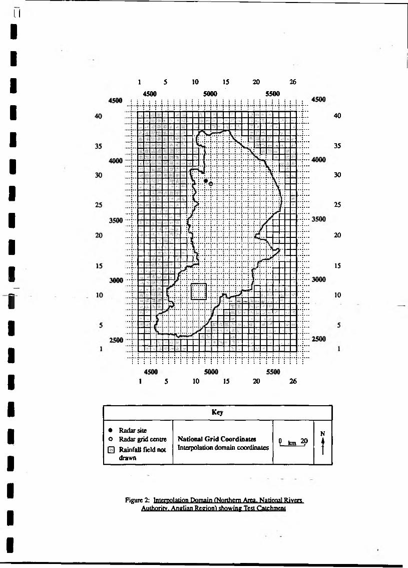
Figure 2 shows the interpolation domain used for the National Rivers Authority, Northern Area.
The boundaries of the rectangular interpolation domain should be set-up so that interpolation takes place over the entire area of interest (regions are invariably not rectilinear but tend to follow political or natural boundaries) Setting up the domain so that it includes the entire area of interest has the advantage of ensuring that the domain remains constant even though the number and locations of raingauge data available may vary.

page 9
5. Program Structure and Data Requirements
This chapter describes the structure of QUANTARE, and the input datafiles it uses.
5.1. Structure
The program consists of small main segment, with most data handling, interaction and graph drawing being handled by subroutines. A full source code listing of QUANTARE is provided in Appendix 1. The program flowchart in figure 3 illustrates the program structure which is also outlined below:
• Character and array initialisation• Welcome message• Run-time Options• Establishment of estimation time period.• Read and process raingauge rainfall data• Data processing and interpolation domain set-up• Main loop• Raingauge rainfall data processing• Interpolation of raingauge rainfall data
Graphical presentation• End of main loop• Write catchment totals to an output file (if required).• Graphical display of cumulated rainfall fields.
5.2. Input and Output Datafiles
The program utilises raingauge rainfall and catchment input datafiles, and files holding coastline and political boundary data.
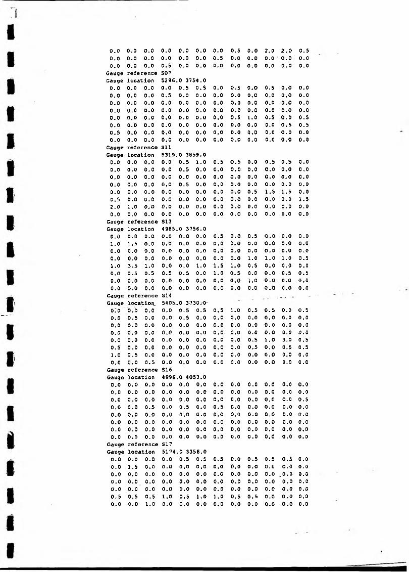
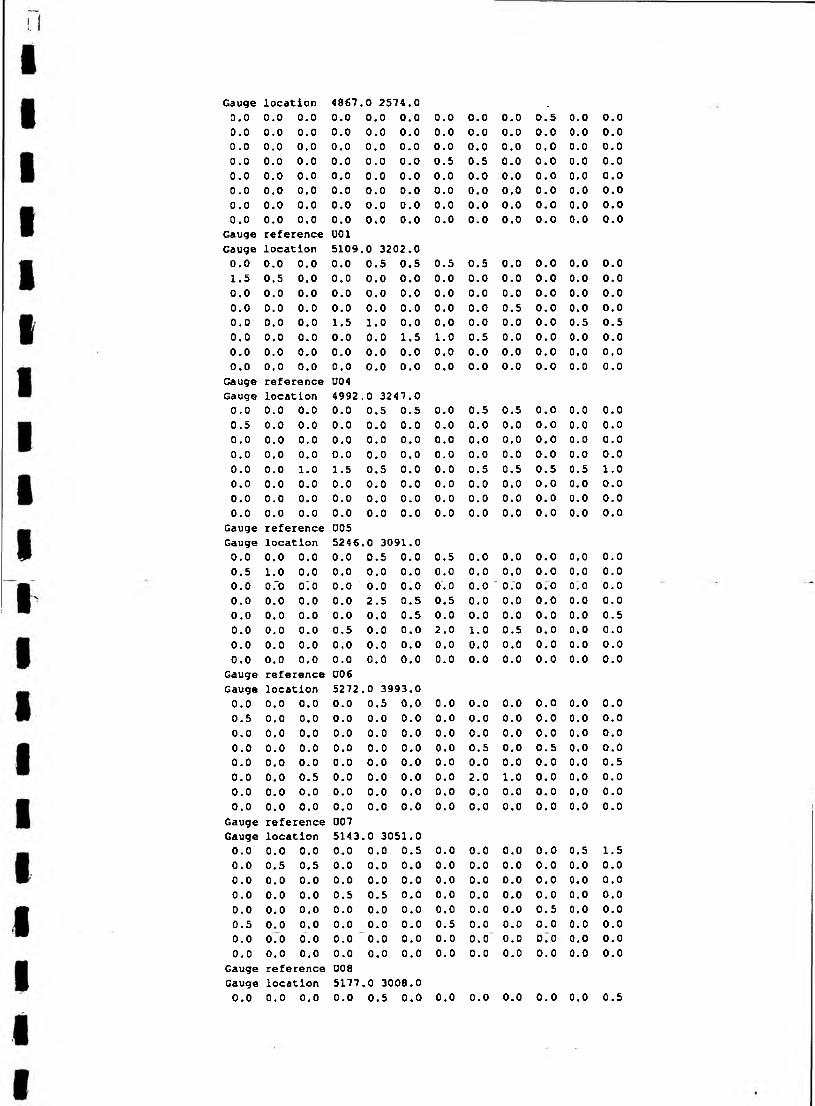
The format of the raingauge rainfall input datafile is shown in figure 4, (an example is listed in Appendix 2) and
the format of a catchment input file is shown in figure 5 (example listed in Appendix 3).
Essentially the raingauge file comprises of 15 minute rainfall depths for a 24 hour period, for all available raingauges in the region. The file has a ten line header block which records the nature of the data, the date,
number of stations, data time period, and data interval. Rainfall data for each raingauge follows sequentially, raingauge after raingauge. Each raingauge has a two line sub-header which shows the raingauge reference code,

page 10
and the gauge location in national grid coordinates.
The catchment inputfile comprises a three-line header block, followed by a catchment number indicator, and then (repeated far each catchment on the datafile), a catchment sub-header (text), catchment node number indicator, and catchment node NGR coordinates.
QUANTARE produces two output files, of which only one is of direct concern. The results output datafile consists of hourly and total rainfall totals for each predefined catchment for the estimation period specified at run-time (see Appendix 5). In addition, the interpolation algorithms sends warning messages to a second output file (for010.dat) when interpolation is taking place for points more than a certain distance from raingauge locations (extrapolation). The messages can be safely ignored (as long as the user is aware of the consequences of extrapolating raingauge data by an interpolating surface) and is advised to delete this file regularly, since it can reach sizable proportions.
5 . 3 . Include File
In order to simplify the program structure, introduce generality, and make application to different areas as straightforward as possible, all the major program parameters are held in a subsidiary include file ‘quantare.inc* (see Appendix 2 for an example). When QUANTARE is being used for the Northern Area referred to throughout this report, the user need only ensure that the correct value of nstcu is used (this value can be changed by editing the include file) and should always be checked before running QUANTARE. Further information on the parameters held in the include file and application of RADGAP to other areas can be found in Chapter 7.
5.4. Presentation of Results
The spatial rainfall field is presented by QUANTARE in the form of two-dimensional colour or black-and-white filled contour plots. The interpolated raingauge rainfall field has depth units (mm).
The rainfall field can be drawn each hour, at the end of the estimation period (or both), the choice being made by the user at run-time. If hourly graphical output is required, two operational modes are accommodated. In the first the user is required to press the return key at the end of each hour before QUANTARE interpolates and displays
data for the next hour, alternatively an auto-refresh option is available whereby the program continues automatically until the end of the estimation period is reached.
page 11
6. Running tbe Program
This chapter describes run-time execution of QUANTARE. A run-time listing of the program user-interface
during run-time is provided in Appendix 6. QUANTARE is straightforward to use and the information required of the user at run-time is limited to a selection of certain run-time options, and the time of the estimation period. Referral to the program flow chart (figure 3) may aid the reader.
6.1. Device T>pe
At present about five devices are supported by QUANTARE for graphical output (i.e. the device names appear in a program menu). However the machine independency of UNIRAS coupled with the large number of device drivers available means that QUANTARE will run on many different device types. If you wish to run QUANTARE on a device not displayed on the program menu contact the Water Resources Research Group indicating the UNIRAS (GROUTE) driver name for the device. This will then be incorporated in the code for a subsequent release version. See Appendix 7 for a list of the devices currently supported.
6.2. Option Menu
There is some flexibility in graphical output produced by QUANTARE. The interpolated rainfall field can be displayed for each hour, or just at the end of the estimation period. If both are required, the user can specify auto refresh whereby the graphical output is automatically updated as data are adjusted. Alternatively, the user is required to press the return key at the end of each hour for the program to continue to the next adjustment hout
6.3. Adjustment Date
The user enters the date for which adjustment is required (in the form YYMMDD). From this information
QUANTARE constructs the name of the raingauge input filename. The estimation period can be of any duration within die 24 hours of the date selected.
6.4. Rainfall Scale Slicing
The user interactively controls the rainfall scale used for the graphical presentation of the interpolated rainfall field. If the hourly graphics option is selected, QUANTARE prompts the user to enter a value for the maximum

page 12
hourly rainfall depth, and likewise for the final cumulated rainfall field at the end of the estimation period. This value corresponds to the top of the rainfall depth scale. From this, QUANTARE computes the scale slice range and sets up the slicing airay. A linear rainfall slicing scheme used with a total of seven rainfall levels. Thus the slice range is computed as the maximum value divided by seven. For example, if the user enters a value of 70 (mm) the rainfall scale will have the values 0*7, 7-14, 14-21,...,63>70. QUANTARE also provides a final ‘catch-all* class of >maximum value. When drawing the final cumulated rainfall field a loop option exists whereby the field can be replotted thereby enabling the user to select a different maximum value (and therefore
different slice range).
6.5. Compiling and Linking RADGAP
When QUANTARE is compiled, the include file is automatically compiled at the same time. It should be ensured that both the main module (quantare.for) and the include file (quantare .inc) are in the same directory. In addition, the interpolation subroutines are held in an object module (alg.obj) which must be linked with the
compiled version of QUANTARE.
6.6. Running QUANTARE
The program is invoked by entering Run quantare . After each response the return (enter) key is pressed, the display scrolls and the next prompt is displayed. The reader is referred to Appendix 6 for the run-time listing.
6.7. Example Run-Time Session
The session shown in the example run-time listing in Appendix S is described below.
RUN QUANTARELaserWriter output device selected.Graphics options settings changed so that graphics are not produced every hout
Auto-refresh selected so that the programs continues automatically until the aid of the estimation period.Default interpolation algorithm used (Renka and Cine).
Black-and-white graphical output selected.The date selected for adjustment is 7th July 1989.The adjustment period selected is from 00:00-24.-00.Maximum rainfall depth selected for graphics scale is 56 (mm). (This will result in the rainfall scale having

page 13
the values 0-8,8*16,16-24,...,48-56, greater than 56).
STOP

r
page 14
7. Customised Implementation of QUANTARE
QUANTARE has been designed and structured so that application to other areas is straightforward. As mentioned
in section 5.3, this has been achieved largely through the use of a FORTRAN include module (‘quantare.inc’). This subsidiary piece of code contains all the major program parameters and enables customisation to be made without altering the code of QUANTARE. The reader should refer to figure 5 for an explanation of the terms and parameters used in this section.
The include file contains a total of 16 parameters and two arrays. An explanatory list of these follows:
cell: interpolation grid size (km)ngrjefjd : ngr coordinates left-side of sub-regionngr_rig_id: ngr coordinates right-side of sub-region
ngrjopjd: ngr coordinates of top of sub-regionngrjfotjd: ngr coordinates of bottom of sub-regionnx: dimension of sub-region (x-axis)ny: dimension of sub-region (y-axis)xlo: - - lower bound of sub^region (x-axis)xhi: upper bound of sub-region (x-axis)
ylo: lower bound of sub-region (y-axis)yhi: upper bound of sub-region (y-axis)idom: number of points outside adjustment domain (ie in mask)start jtop: start and end cells of adjustment domain
nstat: number of raingauge stationsmmax: total number of data points (=nstat+idom)
num_cmt: number of pre-defined catchmentsmaxjtodes: maximum number of nodes allowed in any catchment
The majority of these parameters are self-determining (i.e. they are computed from other parameters entered by
the user), and QUANTARE customisation requires only seven of the parameters on the parameter listing shown above to be amended.
Firstly, the parameter cell should be set. The default and recommended value for this is 5 km, though this can be
changed if a finer or coarser interpolation mesh is required.
The second phase entails setting up a rectangular sub-region. This should be chosen so that there is adequate space for a mask having a depth of not less than least two-cells all the way around the interpolation domain, i.e.
page 15
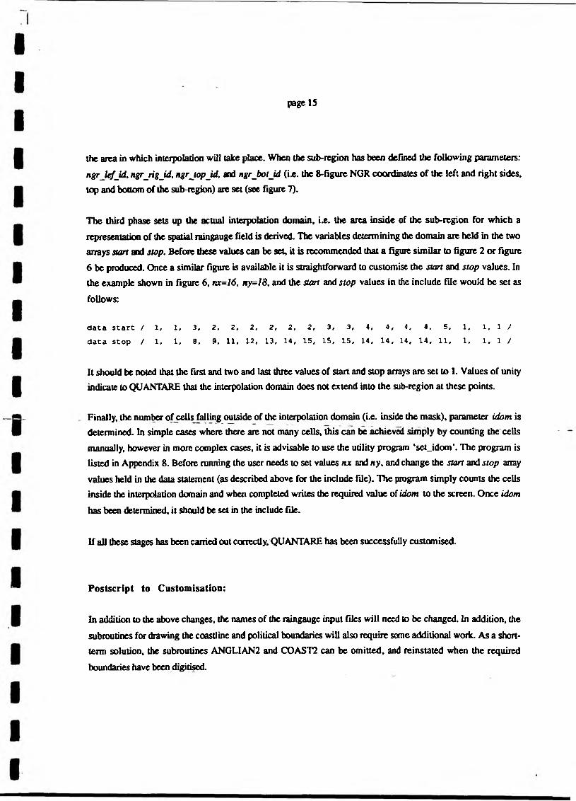
the area in which interpolation will take place. When the sub-region has been defined the following parameters: n g rjr fjd , n grjig jd , ngrjopjd , and ngrjx>t_id (i.e. the 8-figure NGR coordinates of the left and right sides, top and bottom of the sub-region) are set (see figure 7).
The third phase sets up the actual interpolation domain, i.e. the area inside of the sub-region for which a representation of the spatial raingauge field is derived. The variables determining the domain are held in the two arrays start and stop. Before these values can be set, it is recommended that a figure similar to figure 2 or figure6 be produced. Once a similar figure is available it is straightforward to customise the start and stop values. In the example shown in figure 6, nx~16, ny=18, and the start and stop values in the include file would be set as
follows:
data start f 1, 1, 3, 2, 2, 2, 2, 2, 2, 3, 3, 4, 4, 4, 4, 5, 1, 1, 1 / data stop / 1, 1, 8, 9, 11, 12, 13, 14, 15, 15, 15, 14, 14, 14, 14, 11. 1, 1, 1 /
It should be noted that the first and two and last three values of start and stop arrays are set to 1. Values of unity indicate to QUANTARE that the interpolation domain does not extend into the sub-region at these points.
Finally, the number ofcellsfalling outside of the interpolation domain (i.e. inside the mask), parameter idom is determined. In simple cases where there are not many cells, this can be achieved simply by counting the cells manually, however in more complex cases, it is advisable to use the utility program ‘set_idom\ The program is listed in Appendix 8. Before running the user needs to set values nx and ny, and change the start and stop array
values held in the data statement (as described above for the include file). The program simply counts the cells inside the interpolation domain and when completed writes the required value of idom to the screen. Once idom
has been determined, it should be set in the include file.
If all these stages has been carried out correctly, QUANTARE has been successfully customised.
Postscript to Customisation:
In addition to the above changes, the names of the raingauge input files will need to be changed. In addition, the
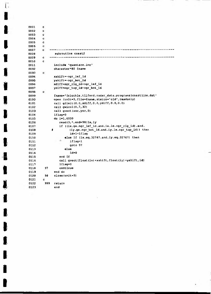
subroutines for drawing the coastline and political boundaries will also require some additional work. As a shortterm solution, the subroutines ANGLIAN2 and COAST2 can be omitted, and reinstated when the required
boundaries have been digitised.
page 16
8. Conclusions
This report is a users guide to the FORTRAN software package QUANTARE, a program for displaying the spatial rainfall field and quantitatively estimating areal rainfall over pre-defined catchments from a network of ground-based raingauges. The report contains listings of full source code and input datafiles; all of which are
contained on the software distribution disk.
QUANTARE is an interactive, user-friendly program featuring user selected options and graphical results presentation. The structure of the program has been described and illustrated using flowchart representation. Data
requirements and input file formats are explicitly described. In addition, full details on customised implementation of QUANTARE to different areas are provided.
A runtime listing is provided and described in the text, and the user options are described.
page 17
Bibliography
Water Resources Research Group References
Cluckie, I.D. and Han, D. (1989). ‘Radar Data Quantisation, Sampling and Preliminary Model Assessment using Upavon Data*, Wessex Radar Information Project, Report no. 4.
Cluckie, I J>. and Tilford, K A . (1988). 'An Evaluation of the Influence of Radar Rainfall Intensity Resolution for Real-Time Operational Flood Forecasting*, Anglian Radar Information Project, Report no. 2.
Cluckie, I.D. and Tilford, K.A. (1989). ‘Transfer Function Models for Flood Forecasting in Anglian Waer Authority*, Anglian Radar Information Project, Report no. 3.
Cluckie, I.D., Yu, P.S. and Tilford, K.A. (1989). ‘Real-Time Forecasting: Model Structure and Data Resolution*, Proc. Seminar on Weal her Radar Networking, Brussels, Belgium, 1989.
Cluckie, I.D., Tilford, K.A., and Shepherd, G.W. (1989). 'Radar Rainfall Quantisation and its Influence on Rainfall Runoff Models’, Proc. Int. Symp. on Hyd. App. o f Weather Radar, University o f Salford, UJC, August.
Cluckie, I.D., Tilford, K.A., and Han, D. (1989). ‘The Influence of Radar Rainfall Quantisation on Flood Forecasting’, //!/. Workshop on Precipitation Measurement, St. Morin, Switzerland, December:
Cluckie, I.D. and Yu, P.S. (1988) ‘Stochastic Models for Real-Time Riverflow Forecasting Utilising Radar Data’, 5th IAHR International Symposium on Stochastic Hydraulics, University o f Birmingham, U.K. August.
Han. D. (1991). Weather Radar Information Processing and Real-Time Flood Forecasting*, Ph.D Thesis, University of Salford, Department of Civil Engineering.
Owens. M.D. (1986). ‘Real-Time Flood Forecasting Using Weather Radar Data*, Ph.D Thesis, University of Birmingham, Department of Civil Engineering.
Tilford. K A (1989a). ‘Software Profile - A User Manual for TFCAL’, University of Salford, Department of Civil Engineering.
Tilford. Kj\ . (1990b). ‘Software Profile - A User Manual for TFUH*, University of Salford, Department of Civil Engineering.
Tilford. K.A. (1989c). ‘Software Profile - A User Manual for AWSTAGE*, University of Salford, Department of Civil Engineering.
Yu. P.S. (1989). ‘Real-Time Grid-Based Distributed Rainfall-Runoff Model for Flood Forecasting with Weather Radar', Ph.D Thesis, University of Birmingham, Department of Civil Engineering.

page 18
Two-Dimensional Interpolation
Cline, AK., and Renka, R.L. (1984) ‘A storage efficient method for construction of a Theissen triangulation’, Rocky Mountain J. Math.% 14,119-139.
Franke, R. and Neilson, G. (1980) Smooth interpolation of large sets of scattered data*, Internal. J. Numtr. Methods Engng., 15,1691-1704.
Lawson, CX. (1977) 'Software for C* surface interpolation'. In: 'Mathematical Software in ’. Rice, J.R. (ed.). Academic Press, New York, 161-194.
Renka, R.L. (1984) 'Algorithm 624: Traingulation and interpolation of arbitrarily distributed data points in the plane', ACM Trans. Math. Software, 10,440-442.
Renka, R.L., and Cline, A.K. (1984) ‘A triangle-based Cl interpolation method*, Rocky Mountain J. Math., 14,223-227.
Other References
Hall, AJ., and Barclay, P.A. (1975) ‘Methods of determing areal rainfall from observed data*, in Prediction in Catchment Hydrology, ed. Chapman X., and Dunin, X., Australia.
Creutin J.D., and Obled, C. (1982) ‘Objective analyses and mapping techniques for rainfall fields: an objective comparison, Water Res. Research, 18 (2 ), 413-431.
(
Display of spatial j rainfall field y
/
Raingauge 1 RaingaugeHate 1 f data
■ —►* f interpolation 1 —^
(scattered I (regulardata) I
*grid)
Figure 1: Schematic representation of the display of spatial rainfall Patterns and the computation of catchment areal rainfall totals
II
1 5 10 15 20 26
4500 5000 5500
40
35
30
25
20
15
10
1 5 10 15 20 26
Key
• Radar site o Radar grid centre03 Rainfall field not
drawn
National Grid Coordinates Interpolation domain coordinates
9 km 2PN
!
Figure 2: Interpolation Domain (Northern Area. National Rivers Authority. Anglian Region! showinp Test Catchment
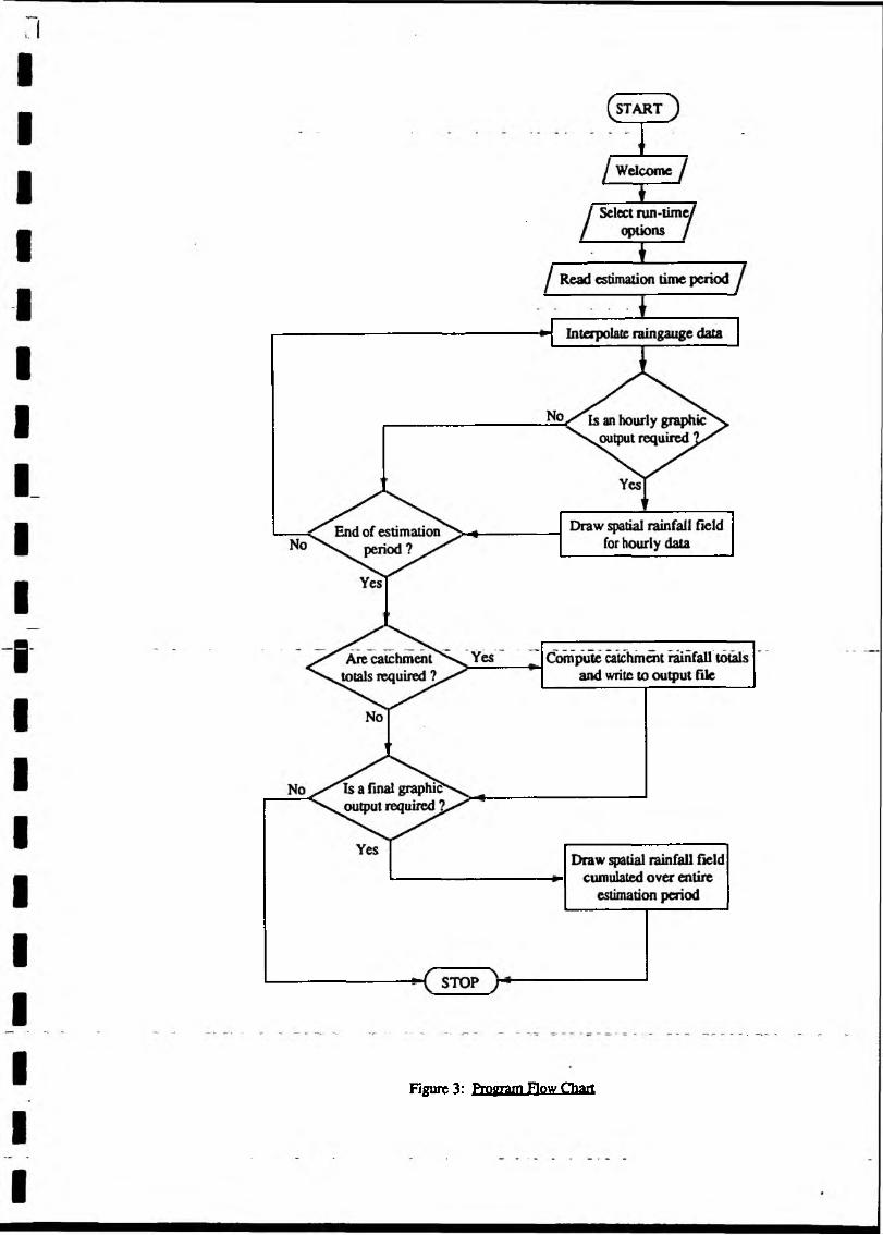
Figure 3: Program Flow Chart

i k
Header block Read as 25x, i2
Sub-header blockI
Data block
96 15 minute rainfall totals per raingauge
{
Raingauge rainfall datafile14 decomber 1989 Number of stations €6Data from 00:00 (first datum) to 23:45 (last datum)15 minute data interval
Read as 21x,a3 Read as 20x, f&l, lx, f6.1
Read as 3x» 12f5.1
Gauge reference 802Gauge location 5552 . 0 3 5 8 6 . 0
0 . 0 0 . 0 0 . 0 0 . 0 0 . 0 0 . 0 0 . 0 0 . 0 0 . 0 0 . 0 0 . 0 0 . 00 . 0 0 . 5 0 . 0 0 . 0 0 . 0 0 . 0 0 . 0 0 . 0 0 . 0 0 . 0 0 . 0 0 . 00 . 0 0 . 0 0 . 0 0 . 0 0 . 0 0 . 0 0 . 5 0 . 0 1 . 0 0 . 5 0 . 5 0 . 00 . 5 0 . 5 0 . 5 0 . 5 0 . 5 0 . 0 0 . 5 0 . 0 0 . 0 0 . 5 0 . 5 0 . 00 . 5 0 . 0 0 . 5 0 . 0 0 . 0 0 . 0 1 . 5 2 . 5 2 . 5 1 . 5 1 . 0 0 . 50 . 0 0 . 5 0 . 0 0 . 0 0 . 0 0 . 0 0 . 5 0 . 0 0 . 0 0 . 5 0 . 0 0 . 00 . 0 0 . 0 0 . 0 1 . 0 0 . 5 0 . 5 1 . 0 0 . 5 0 . 0 0 . 0 0 . 0 0 . 50 . 5 0 . 0 0 . 5 0 . 0 0 . 0 0 . 0 0 . 0 0 . 0 0 . 0 0 . 0 0 . 0 0 . 0Gauge reference 803Gauge 11 location 5106 . 0 3 6 9 8 . 0
0 . 0 , 0 . 0 0 . 0 0 . 0 0 . 0 0 . 0 0 . 0 0 . 0 0 . 0 0 . 0 0 . 0 0 . 00 . 5 0 . 0 0 . 0 0 . 5 0 . 0 0 . 0 0 . 0 0 . 0 0 . 0 0 . 0 0 . 0 0 . 00 . 0 , 0 . 0 0 . 0 0 . 0 0 . 0 0 . 0 0 . 0 0 . 5 0 . 5 0 . 0 0 . 5 0 . 50 . 5 0 . 5 0 . 5 0 . 0 0 . 5 0 . 5 1 . 0 0 . 0 0 . 5 0 . 5 0 . 5 0 . 51 . 0 0 . 0 0 . 5 0 . 0 0 . 5 0 . 0 0 . 0 0 . 0 1 . 0 0 . 0 0 . 0 0 . 50 . 0 0 . 5 0 . 0 0 . 0 0 . 0 0 . 0 0 . 0 0 . 0 0 . 0 0 . 5 0 . 0 0 . 00 . 0 ' 0 . 0 0 . 5 0 . 5 1 . 0 0 . 5 0 . 5 0 . 5 1 . 0 0 . 5 0 . 5 0 . 50 . 5 0 . 0 0 . 0 0 . 0 0 . 0 0 . 0 0 . 0 0 . 0 0 . 0 0 . 0 0 . 0 0 . 0
Figure 4: Example fainfall datafile (items read bv QUANTARE in bold)

1.1
ngr_top_id19
18
17
16
15
14
13
12
11
10
9
8
7
65
4
3
2
1ngr_bol_id
ngr_lefjd *
i i i i i i i i « • ' < *
2 3 4 5 6 7 8 9 10 11 12 13 14 15 16ngr_rig_id
-------------------------------------— nx-----------------------------------------------------►
Figure 5: Sub-Region and Interpolation Domain

I
IIi
Appendix 1 Source Code ListingAppendix 2 Include FileAppendix 3 Example Raingauge Rainfall InputfileAppendix 4 Example Catchment InputfileAppendix 5 Example OutputfileAppendix 6 Runtime ListingAppendix 7 Devices SupportedAppendix 8 Utility Program Source Listing (set_idom)
Appendices

Appendix 1: Source Code Listing
0001 c0002 c0003 c0004 c0005 c PROGRAM QUANTARE0006 c0007 c A program for estimating areal rainfall depths from point raingauge0008 c rainfall data. The irregularly distributed raingauge rainfall amounts0009 c are interpolated to a regular (5 km * 5km) grid by a sophisticated0010 c two-dimensional interpolation algorithm.0011 c0012 c Water Resources Research Group0013 c Department of Civil Engineering0014 c University of Salford0015 c SALFORD0016 c M5 4WT0017 c0018 c For further information contact:0019 c Prof. Ian Cluckie0020 c0021 c0022 c0023 c0024 c0025 program quantare0026 c0027 c IMPORTANT, before running check settings of parameters in include file0028 c ’quantare.inc', especially snstat (number of raingauges) .002 9 c0030 include 'quantare.inc10111 c , ■ - - - ...0112 real rg_interp(nx, ny), cum_rg_interp (nx,ny)0113 real x(nstat),y(nstat), f(nstat),cum_rg(nstat),value(nstat,96)0114 real px(nx),py(ny)0115 real fnodes (5*nstat>,wrk(6*nstat)0116 real out(nx,ny),array(nx,ny)0117 character*3 gr(nstat)0118 character*l opt1,opt2, opt3, opt4,opt6,replot0119 character*6 day0120 integer kh,istart_hour, iend_hour,idev,icount,icol0121 c0122 real cmt_x(num_cmt),cmt_y(num_cmt)0123 integer icmt_x (num_cmt, max_nodes), icmt_y (num_cmt, max_nodes)0124 integer nnodes(max_nodes)0125 real cmt_hour_rf(num_emt,24)0126 character*60 cmt_name(num_cmt)0127 c0128 icount-10129 c0130 c0131 c0132 c0133 c type welcome message0134 c0135 call welcome0136 c0137 c0138 c0139 c get graphics device and other options

0140 c0141 call options(idev,optl,opt2,opt3,opt4/icol,opt 6) - -0142 c0143 c -------------------------------------------------------------0144 c0145 c call subroutine to read and process raingauge data0146 c0147 call rg_read(day,x,y,value,gr,cum_rg,istart_hour,iend_hour) 0146 c0149 c -------------------------------------------------------------0150 c0151 c call subroutine to read catchment data0152 c0153 if (opt6.eq.'Y') then0154 call cmt_read(neat,nnodes,icmt_x,icmt_y,cmt_name)0155 do j-l,ncat0156 do i-1,240157 cmt_hour_rf(j,i)-0.00158 end do0159 end do0160 end if0161 c0162 c ------------------------------------------------------------0163 c0164 c call subroutine to determine adjustment domain0165 c0166 call setup_domain(px,py>0167 c0168 c -------------------------------------------------------------0169 c0170 c0171 c main loop0172 c
0174 do kh“istart_hour,iend_hour0175 c ----------------------- — — --— -- —0176 c0177 c0178 c ------------------------------------------------------------0179 c0180 c set •f• array to have rainfall data for correct hour inside0181 c0182 do kk-l,nstat0183 f(kk)-0.00184 end do0185 jj»((kh-1)*4)+10186 do kk*l,nstat0187 do i-jj.jj + 30188 f(kk)-f(kk)+value(kk, i)0189 end do0190 end do0191 c0192 c ------------------------------------------------------------0193 c0194 if (kh«eq.istart_hour) then0195 write(*, *)0196 w r i t e )* ---------------------------------------0197 #----------------------- ’ - ,0198 write (*, *)0199 write(*,*J* Computation segment*0200 write <*, *)0201 write(*,M • ---------------------------------------

0202 #----------------------------------- '0203 _ write(*, M0204 end if0205 write <*,*)0206 write(*,M' Computing for hour ' ,kh0207 write<*, M * -------------------------------------- '0208 c0209 c -------------------------------------------------------------------0210 c0211 c two algorithms are available to interpolate raingauge data to a0212 c regular grid.0213 c0214 if (opt4.eq.'A*) call0215 # rg_interpolatel(x,y, f , px,py, rg_interp)0216 if <opt4.eq.'B') call0217 t rg_interpolate2(x,y, f,px,py,rg_interp)0218 c0219 c -------------------------------------------------------------------0220 c0221 c compute hourly catchment rainfall totals0222 c0223 if (opt6.eq.'Y 1) then0224 do j«l,ncat0225 do i»l,nnodes(j)0226 cmt_hour_rf (j, kh) “cmt_hour_rf (j, kh) +0227 t rg_interp <icmt_x (j, i) ,icmt_y (j, i) )0228 end do0229 cmt_hour_rf ( j, kh) -cmt_hour_rf ( j, kh) /real (modes ( j) )0230 end do0231 end if0232 c0233 c -------------------------------------------------------------------0234 c0235 c update arrays for cumulating interpolated raingauge arrays "0236 - c -0237 do i-1,nx0238 do j“l,ny0239 cum_rg_interp(i, j)«cum_rg_interp(i, j) +rg_interp(i, j)0240 end do0241 end do0242 c0243 c -------------------------------------------------------------------0244 c024 5 c rg_interp cells outside adjustment domain are assigned0246 c a value of -999.999 so that they are not plotted0247 c024 8 call outside_boundary3 (rg_interp)0249 c0250 c -------------------------------------------------------------------0251 c0252 c if required call graphics routines to plot hourly adjustment0253 c0254 if (optl.eq.*Y') call0255 # graphics(ieount,idev, icol, kh,istart_hour,x, y, rg_interp)0256 c0257 c -------------------------------------------------------------------0258 c0259 c0260 if (optl.eq.'Y*.and.opt3.eq.'N') then ̂ "0261 write(*,*)' Press return to continue...'0262 read(*,*)0263 write(*,*) ’ •

02 64 end if0265 c0266 c0267 c ==0268 end do ! end of main loopVZ D70270 c0271 c0272 c0273 C “■0274 c0275 c write catchment rainfall totals to an output file0276 c0277 if (opt6.eq.'Y') then0278 do j-l,ncat0279 cmt_total-0.00280 write(9,20)cmt_name< j)0281 do ihour«istart_hour,iend_hour0282 write(9, 27)ihour,cmt_hour_rf(j, ihour)0283 cmt_total”cmt_total+cmt_hour_rf(j,ihour)0284 end do0285 write{9,29)cmt_total0286 write(9,*)' •0287 end do0288 write(9,*)' '0289 write (9, *) ' ---------------- End of file --------------- '02 90 end if02 91 27 format<3x,i2,1)*,4x,f5.2)02 92 28 format(a60)0293 29 format{3x,'Total *,lx,f6.2)02 94 c0295 C ™ “0296 c0297 c if required process data and call graphics routines to plot final-0298' ~ C adjustment fields" _ _ .0299 c0300 call outside boundary3(cum rg interp)0301 write(*,*)0302 write(*,*)' Please wait, preparing final graphics...'0303 if (opt2.eq.*Y') then0304 36 call graphics(icount,idev,icol,99,istart_hour,x,y,cum_rg_interp)0305 write(*,*)' ■0306 13 write(*,*)' Do you wish to replot the rainfall field (Y/N) ?‘0307 read(*,12,err-13)replot0308 if (replot.ne.'y'.and.replot.ne.'Y'.and.0309 4 replot.ne.'n'.and.replot.ne.'N') goto 130310 if (replot.eq.'y'.or.replot.eq.*Y') goto 360311 write(*,*) ' '0312 end if0313 12 format(al)0314 c0315 c0316 c0317 c0318 write(*,*)0319 write(*,*)0320 write (*,*)* ---------------------------- QUANTARE STOP0321 # ------------------------------- '0322 - write<*,*) " “ ‘ ‘ ‘ ‘ -0323 write<*,*)0324 call gclose0325 end
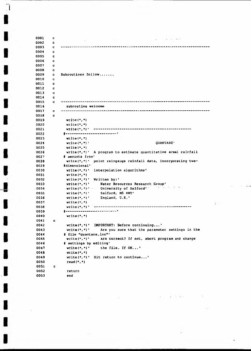
0001 c - -0002 c0003 c0004 c0005 c0006 c0007 c0008 c0009 c Subroutines follow......0010 c0011 c0012 c0013 c0014 c0015 c0016 subroutine welcome0017 c0018 c0019 write(*,*)0020 write(*,*)0021 i ̂ a / 4 k Iwrite i * j0022 i------------0023 write(*,*)0024 write (*, *)' QUANTARE *0025 write (*,M0026 write(*,*) ' A program to estimate quantitative areal rainfall0027 t amounts from I0028 write(*,*) ' point raingauge rainfall data, incorporating two-0029 ♦dimensional'0030 write{*,*) ' interpolation algorithms'0031 write(*, *)0032 write{*,*) ' Written by:'0033 write (*,*)* Water Resources Research Group*0034 write (*, *■)•*- - University of Salford'0035 write(*, *) ' Salford, M5 4WT*0036 write (*,*) ' England, U.K.'0037 write (*,*)0038 wricG ( f j0039 #------------0040 write(*,*)0041 c0042 write(*,*) ' IMPORTANT: Before continuing...'0043 write <*,*)* Are you sure that the parameter settings in the0044 # file "quantare.inc"’0045 write (*,*)' are correct? If not, abort program and change004 6 I settings by editing'0047 write(*,»)' the file. If OK...'0048 write(*,*)0049 write(*,*) • Hit return to continue...*0050 read(*,*)0051 c0052 return0053 end

0001000200030004000500060007000800090010001100120013001400150016001700180019002000210022002300240025002600270028002900300031003200330034
-0035003600370038003900400041004200430044004500460047004800490050005100520053005400550056005700580059006000610062
cccccc ---------------------------------------------------------------
subroutine options(idev,setl, set2,set3,set4,icol,set6)c ----------------------------------------------------------------c
character*! setl,set2,set3,set4,set5,set6 integer opt,icol
c35 format <il>45 format (al)
cwrite <*,M write (*,*)write(*,*)' ---------------------------------------------
I -----------------------------------•write (*,M* The UNIRAS graphics routines in this program are
t device independent.'write (*, *)* ---------------------------------------------
#-----------------------------------'write (*,M
696 write(*,*)' Please type in the integer corresponding to the I device required*write(*, M * (1) VAXstation (GPX driver)'write (*, M ’ (2) VAXstation (Xll driver)'write(*, M ’ (3) VT Emulator (ReGIS driver) 1write(*, *> ' (4) IBM PC (VGA driver)’write(*,*) ' (5) Inkjet Printer*write(*, M ' (6) LaserWriter (Postscript)'write (*, *)write( Please type integer 11,2,3,4,5 or 6]
read(*,*, err-31)idevif (idev .gt.6.or.idev.eq.0) goto 31write(* *)
setl-1Y *set2-'Yset3-'Yset4“ 1Aset5-'Cset 6-* Yicol*lwrite{* *)write (* *)write (* *)write (* *1
write {* *) 1 Option Menu*write(* *11*1
write (* *)write(* •) ' Options (default in UPPER CASE)'write (* *)write (* *) • 1. Graphics every hour (Y/n) •write (* *) • 2. Graphics at end of period (Y/n)■write (* *> ' 3. Auto refresh (Y/n) ■write (* *) ' 4. Interpolation algorithm (enter a or b) : •write(* *) ' (a) Renka and Cline (default) *write(* *) * (b) Modified Shepherd'

0063 write(*,*)' 5. Colour or black/white graphics __ (C/b)0064 write(*,*)’ 6. Compute catchment rainfall totals (Y/n)'0065 5 write (*, *)0066 write(*,*)' To change a default setting enter integer0067 t corresponding to the setting*0068 write(*,*)' to be changed, press return key and enter y or0069 < as appropriate'0070 25 write(*,*)’ (Enter 0 <rtn> to continue]...'0071 26 write(*,*)0072 read(*,35,err-25)opt0073 if (opt.ne.l.and.opt.ne.2.and.opt.ne.3.and.opt.ne.4.0074 f and.opt.ne.5.and.opt.ne.6.and.opt.ne.0) then0075 writet*,*)' Enter integer [1,2,3,4,5,6 or 0]...’0076 goto 250077 end if0078 if (opt.eq.0) then0079 goto 150080 else if (opt.eq.l) then0081 read(*,45)setl0082 if (setl.eq.'y') setl-'Y'0083 if (setl.eq.'n') setl-'N*0084 else if (opt.eq.2) then0085 read(*,45)set20086 if (set2.eq.'y’> set2-'Y’0087 if (set2.eq.*n') set2«'N'0088 else if (opt.eq.3) then0089 read(*,45)set30090 if (set3 .eq. *y *) set3**'Y'0091 if (set3.eq.'n') set3»'N'0092 else if (opt.eq.4) then0093 read(*,45)set40094 if (set4.eq.'a') set4='A'0095 _ if (set4.eq.'b'> set4«'B’0096 else if (opt.eq.5) then ‘ ~ -0097 read(*,45)set50098 if (setS.eq.'c'.or.sets.eq.'C') icol"l0099 if (set5.eq.'b'.or.set5.eq.'B') icol*30100 else if (opt.eq.6) then0101 read(*,45)set60102 if (set6.eq.'y*> set6"'Y'0103 if (set6.eq.'n ') set6-'N'0104 else0105 write(*,*)* Error in options module*0106 end if0107 goto 260108 15 continue0109 c0110 return0111 end

0001 c0002 c0003 c0004 c0005 c0006 subroutine cmt_read (neat, nnodes, icrat_x, icmt_y, cmt_name)0007 c0008 c0009 include 'quantare.inc'0090 real cmt_x (num_cmt, max_nodes), cmt_y (num_cmt, max_nodes)0091 integer icmt x (num_cn\t, max_nodes), icmt_y (num_cmt, max_nodes)0092 integer nnodes(max_nodes)0093 character*60 cmt_name(num_cmt)0094 c0095 open(unit-8, name-'quantare.cmt',status-'old',readonly)0096 do i**l,30097 read(8,*>0098 end do0099 read(8,*)neat0100 type*,neat0101 do j-l,ncat0102 read{8,11)cmt_name(j)0103 read(8,*)nnodes(j)0104 do i-1,nnodes (j)0105 read(8, *> cmt_x(j,i),cmt_yt j,i)0106 iemt_x(j, i)-1+ < <cmt_x(j, i)-ngr_lef_id)/50.0)0107 icmt_y(j, i)-1+((cmt_y(j, i)-ngr_bot_id)/50.0)0108 end do0109 end do0110 close(unit»8)0111 11 format(a60)0112 c0113 ■ open(unit»9,name*’rainfall.out',status-'new')0114 write(9,*)' '0115 . write(9,*)* ----------------------------------- ------- 10116 write(9,*)' QUANTARE Output File: Catchment rainfall totals’0117 write(9,*) ' --------------------------------------------'0118 write(9, *) ' '0119 write(9,M' Hourly rainfall totals:'0120 write (9, *) ' --------------------- '0121 write(9,*)' '0122 write(9,*)' Hour: Rainfall (mm):'0123 c0124 return0125 end
000100020003000400050006
ccccc
• - •
00070008
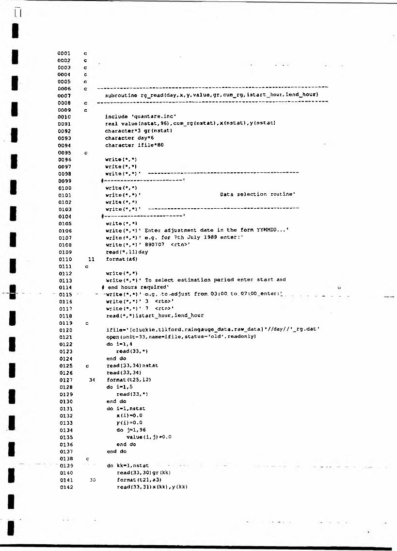
subroutine rg_read(day,x,y,value,gr,cum_rg,istart_hourr iend_hour)
0009 c0010 include 'quantare.inc’0091 real value(nstat,96), cum_rg(nstat),x(nstat),y{nstat)0092 character*3 gr(nstat)0093 character day*60094 character ifile*800095 c0096 write (*,*)00970098
write (*,*)write(*,*)' — ---------- ----- — ~
00990100 write (*,*)0101 write{*,*)' Data selection routine’01020103
write(*,*)write{*,M ' ----------------------- ” ~
01040105 write (*,*)0106 write(*,*)’ Enter adjustment date in the form YYMMDD... ’0107 write(*,*>' e.g. for 7th July 1989 enter:'0108 write (*,*)* 890707 <rtn>'0109 read(*,11)day0110 11 format(a6)0111 c0112 write (*,*)0113 write {*,*)' To select estimation period enter start and0114 # end hours required'0115 - - -write (*,*)' e.g.-to-ad just from.-03 :00. to. 0.7 :.00_enter: _0116 write (*,*>' 3 <rtn>'0117 write (*,*)' 7 <rtn>'0118 read(*,*)istart^hour, iend_hour0119 c0120 ifile-’[cluckie.tilford.raingauge_data.raw_data] ‘//day//'_rg.dat10121 open(unit-33,name-ifile,status—'old',readonly)0122 do i-1,40123 read(33,*)0124 end do0125 c read(33,34)nstat0126 read(33,34)0127 34 format(t25,i2)0128 do i-1,50129 read{33, *)0130 end do0131 do i-1,nstat0132 x(i)“0.00133 y<i)*0.00134 do j*l»960135 value(i,j)*0.00136 end do0137 end do0138 c0139 - - - do kk-1,nstat - - - - - - — ̂ ̂ -0140 read(33, 30) gr (kk)0141 30 format(t21,a3)0142 read(33,31)x{kk), y(kk)

0143014401450146014701480149015001510152015301540155015601570156
31 format(t20,f6.1,lx,f6.1)x(kk)-(x(kk)-ngr_lef_id)/50.0 y (kk)- (y(kk)-ngr_bot_id)/50.0 k-1do 1-1.96/12
read(33,16)(value(kk,j),j-k,k+ll) k-k+12
end do16 format(3x,12f5.1)
end dodo kk-1,nstat
do i-1,96cum_rg(kk)-cum_rg(kk)+value(kk,i)
end do end do
creturnend
00010002
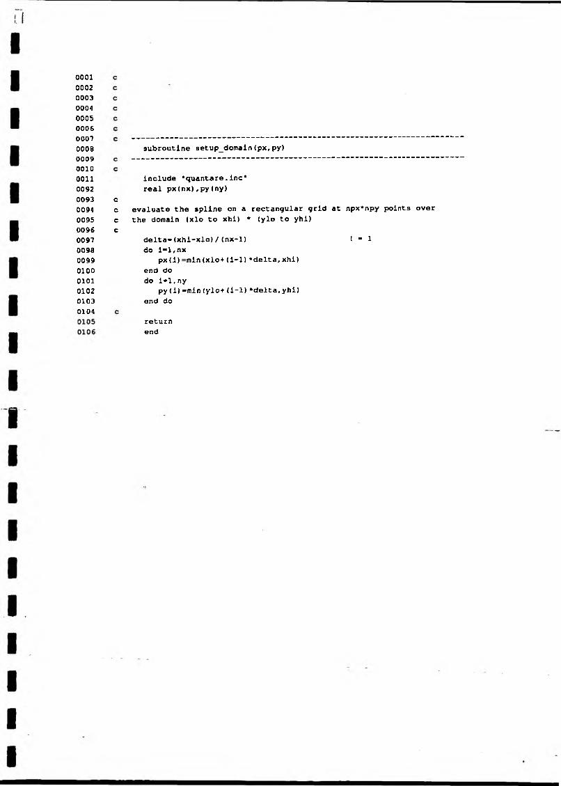
00030004000500060007oooe00090010
00110092009300940095009600970098009901000101010201030104
subroutine setup_domain(px,py)
c
include 'quantare.inc' real px(nx),py(ny)
cc evaluate the spline on a rectangular grid at npx*npy points over c the domain (xlo to xhi) * (ylo to yhi)
delta-(xhi-xlo)/(nx-1) ! ” 1do i-l,nx
px(i)=min(xlo+ <i-l)*delta,xhi) end do do i«l,ny
py(i)-min(ylo+(i-1)*delta,yhi) end do
returnend

000100020003000400050006000700080009001000110012001300940095009600970098009901000101010201030104010501060107010801090110011101120113011401150116011701180119
C
ccccc ---------------------------------------------------------------
subroutine rg_interpolatel(x,y,z,px,py,rg_interp)c ---------------------------------------------------------------cc this routine interpolates raingauge data after a modified c Renka and Cline routine c
include ’quantare.inc * integer triang(7*nstat),ifailreal grads(2,nstat),px(nx),py(ny),rg_interp(nx,ny) real x (nstat),y(nstat),z(nstat)
ccc interpolation of raingauge data to a regular grid c generate triangulation and gradients c
ifail-0write(*,*)’ Please wait, computing interpolating function...* call eOlsae(nstat,x,y, z, triang,grads,ifail) call x04aae(l,10)write(*,*)' Please wait, evaluating interpolant' writet*,*)' ' do j«ny,l,-l
do i-l,nx ifail— 1 call eOlsbe
# (nstat,x,y, z,triang,grads,px(i),py(j),rg_interp(i, j) , ifail)end do
end doc
do i-l,nx do j=l,ny
if (rg_interp(i, j) .It.0.0) rg_interp(i,j)=0.0 end do
end doc
returnend
0001 c0002 c0003 c0004 c00050006
cc
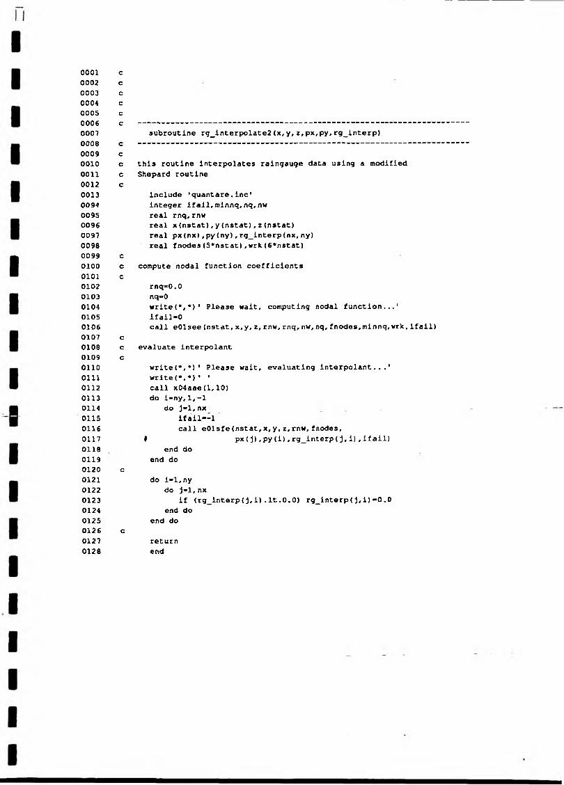
00070006
subroutine rg_interpolate2(x,y,z,px,py,rg_interp)c
0009 c0010 c this routine interpolates raingauge data using a modified0011 c Shepard routine0012 c0013 include 'quantare.inc'0094 integer ifail,minnq,nq,nw0095 real rnq,rnw0096 real x(nstat),y(nstat),z(nstat)0097 real px(nx),py(ny),rg_interp(nx,ny)0098 real fnodes(5*nstat),wrk(6*nstat)0099 c0100 c compute nodal function coefficients0101 c0102 rnq»0.00103 nq®00104 write(*,*>' Please wait, computing nodal function...'0105 ifail-00106 call eOlsee(nstat,x,y, z, rnw,rnq,nw,nq, fnodes, minnq, wrk,ifail)0107 c0108 c evaluate interpolant0109 c0110 write(*,*)' Please wait, evaluating interpolant...'0111 write(*,*>' ’0112 call x04aae (1,10)0113 do i-ny,1,-10114 do j-l,nx0115 ifail--l0116 call eOlsfe(nstat,x,y,z,rnw,fnodes.0117 # px(j),py(i),rg_interp(j, i) , ifail)0118 end do0119 end do0120 c0121 do i-l,ny0122 do j=l,nx0123 if (rg_interp(j,i).It.0.0) rg_interp(j,i)-0.00124 end do0125 end do0126 c0127 return0128 end

000100020003000400050006000700080009001000110012009300940095009600970098009901000101
010201030104010501060107010801090110011101120113011401150116011701180119012001210122
012301240125012601270128012901300131013201330134013501360137
subroutine outside boundary3(array)
c
include ’quantare.inc' real out{nx,ny),array(nx,ny)
do i-l,nyif (.not.(start(i).eq.1.and.stop(i).eq.1)) then
mas)c_stop“i+l goto 5
end if5 end do
do i**l,nyif (.not. {start(i).eq.1.and.stop(i).eq.1)) then
mask_start”i-l goto 6
end if end do
6 continue
do i-mas)c_start+l,mask_stop-l do j=l,start (i)
out (j, i) -10.0 end dodo j-stop(i),nx
out (j, i) =10.0 end do
end dodo i-l,mask_start
do j=l,nxout ( j, i) “10.0
end do end dodo i*mask_stop,ny
do j“l,nxout(j,i)“10.0
end do end do
k“ldo i-l,nx
do j=l,nyif (out(i, j) .eq.10.0) array (i. j)— 999.999
end do end do
returnend
0001 c0002 c - -0003 c00040005
cc
00060007
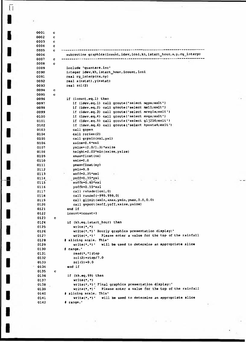
subroutine graphics (icou'nt, idev, icol,kh, istart_hour, x,y, rg_interp>c
oooe c0009 include •quantare.inc'0090 integer idev, kh, istart_hour, icount,icol0091 real rg_interp(nx,ny)0092 real x(nstat),y{nstat)0093 real zcl(2)0094 c0095 c0096 if (icount.eq.l) then0097 if (idev.eq.l) call groute('select rogpx;exit')0098 if (idev.eq.2) call groute('select mxll;exit')0099 if (ldev.eq.3) call groute(1 select mregis;exit’)0100 if (idev.eq.4) call groute ('select mvga;exit')0101 if (idev.eq.5) call groute{*select glj250;exit')0102 if (idev.eq.6) call groute('select hposta4;exit*)0103 call gopen0104 call rorien(2)0105 call grpsiz(xsi,ysi)0106 xsize*0.4 *xsi0107 ysize*(2. 0/1.3)*xsize0100 height-0.03*min(xsize,ysize)0109 xmax=fleat(nx)0110 xmin-0.00111 ymax-float(ny)0112 ymin*0,00113 xoff-0.35*xsi0114_ yoff-0.35*ysi0115* xoffk»0.65*xsi0116 yoffk«0.15*xsi0117 call rshade(icol, 0)0118 call rundef(-999.999,0)0119 call glimit(xmin,xraax,ymin,ymax,0.0, 0.0)0120 call gvport(xoff,yoff,xsize,ysize)0121 end if0122 icount»icount+l0123 c0124 if (kh.eq.istart_hour) then0125 write(*,*)0126 write(*,*)' Hourly graphics presentation display:'0127 write(*,*)' Please enter a value for the top of the rainfall0128 t slicing scale. This*0129 write(*,*)' will be used to determine an appropriate slice0130 # range.*0131 read(*,*)ztop0132 zcl(2)-ztop/7.00133 zcKD-0.00134 end if0135 c0136 if (kh.eq.99) then0137 write(*,*)0138 write{*,*)' Final graphics presentation display:'0139 write(*,*)' Please enter a value for the top of the rainfall0140 # slicing scale. This'0141 write(*,*)' will be used to determine an appropriate slice0142 ♦ range.'
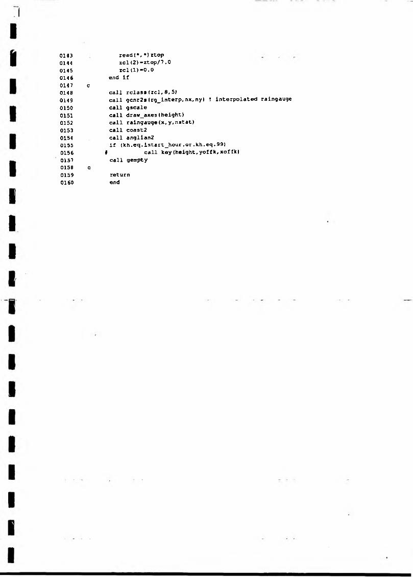
0143 read(*,*)ztop014 4 zcl(2)-ztop/7.00145 zcMD-0.00146 end if0147 c0148 call rclass(zcl,8,5)014 9 call gcnr2s(rg_interp,nx,ny) ! interpolated raingauge0150 call gscale0151 call draw_axes(height)0152 call raingauge(x,y,nstat)0153 call coast20154 call anglian20155 If (Xh.eq.i3tart_hour.or.kh.eq.99)0156 # call key(height,yoffk,xoffk)0157 call gempty0158 c0159 return0160 end

0001 c0002 c0003 c0004 c00050006
cc
00070008
subroutine draw_axes(height)c
0009 c0010 parameter (gundef **999. 999, iundef -9999, undef-0.0)0011 real north,south,east,west0012 integer lenarl(4)0013 character*14 texarl(4)0014 c0015 east-■5700.00016 vest*'4 400.00017 north1-4400.00018 south1-2400.00019 data lenarl / 0,13,0,14 /0020 data texarl / ' Easting (NGR) ', ' ^'Northing (NGR) ' /0021 data dbl,ntick / 1000.0,4 /0022 c0023 call glimit(west,east,south, north,0.0,0.0)0024 call raxtef(6,'SWIM',1)0025 call raxlfo(0,0,iundef,iundef)0026 call raxbti(6,gundef,gundef,dbl)0027 call raxsti(ntick)0028 call raxdis(4,1, iundef)0029 call raxdis(3,1,iundef)0030 call raxdis(6,1,iundef>0031 call raxis2(south,west,height,lenarl,texarl)0032 call raxis (1,north,height,2)0033 call raxdis(4,0, iundef)0034 call raxis(2,east,height,2)0035 c0036 return0037 end
00010002000300040005oooe000700080009001000110092009300940095009600970098009901000101010201030104010501060107010801090110
011101120113011401150116011701180119012001210122
ccccccc ---------------------------------------------------------
subroutine coast2c ---------------------------------------------------------c
include 'quantare.inc’ character*80 fname
cxshift— ngr_lef_idyshift»-ngr_bot_idxdiff-ngr_rig_id-ngr_lef_idydi f f-ngr_top_id-ngr_bot_id
cfname-'[cluckie.tilford.radar_data.programsJ coastline.dat'open (unit-3,file-fname,status-'old',readonly)call glimit(0.0,xdiff,0.0,ydiff,0.0,0.0)call gwicol(0.7,32)call gvect(xor,yor,0)iflag-0do i»l,6000
read(3,*,end-98)ix,iyif ((ix.ge.ngr_lef_id.and.ix.le.ngr_rig_id).and.
# (iy.ge.ngr_bot_id.and.iy.le.ngr_top_id)) thenid-l-iflag
else if (ix.eq.32767.and.iy.eq.32767) then if lag*=l goto 97
else id-0
end ifcall gvect(float(ix)+xshift, float(iy)+yshift,id) iflag-0
97 continue end do
98 close(unit-3)c999 return
end

00010002
000300040005C00600070008000900100091009200930094009500960097009800990100010101020103010401050106010701080109011001110112011301140115011601170118011901200121
012201230124012501260127012B0129013001310132013301340135013601370138013901400141
cccccc ----------------------------------------------------------
subroutine anglian2c ----------------------------------------------------------c
include ’quantare.inc’integer ix(6000),iy(6000),icolour(6000) real ngr_x<6000),ngr_y(6000) real ang_ngr_xmax (6), ang_ngr_xmin(6) real ang_ngr_ymax(6), ang_ngr_ymin(6) character*80 fname (6)
cxshift**-ngr_lef_id yshift— ngr_bot_id xdif f-ngr_rig_id-ngr_lef_id ydiff-ngr_top_id-ngr_bot_id
cfname(1)='Icluckie.tilford.dig)anglian_inland_boundary. map'fname(2)-'[cluckie. tilford.dig]lobound.map'fname( 3 ) [cluckie. tilford.dig]ocbound.map'fname(4)=*[cluckie.tilford.digJncbound.map'fname(5)-'Icluckie.tilford.dig)nor_only_bound.map'
cdo k-1,5
open (unit-3, file-fname(k), status**1 old', readonly)num_data-0ixmax-0iymax~0ixmin-10000iymin-10000do i-1,6000
read{3,*,end-98)ix (i),iy(i), icolour(i) if (ix(i).gt.ixmax) ixmax=ix(i) if (iy(i).gt.iymax) iymax-iy(i) if (ix(i).lt.ixmin) ixmin-ix(i) if (iy(i).lt.iymin) iymin-iy(i) num_data=num_data+l
end do98 ang_ymax-float (iymax)
ang_ymin-float(iymin) ang_ngr_ytnax (1) —4250. 0 ang_ngr_ymin11)-1750.0 ang_ngr_ymax(2)-3390.0 ang_ngr_ymin {2) -317 0.0 ang_ngr_ymax (3) -3270.0 ang_ngr_ymin(3)-2520.0 ang_ngr_ymax(4)-3420.0 ang_ngr_ymin(4)-2290.0 ang_ngr_ymax(5)-2580.0 ang^_ngr_ymin (5)=2340.0 ang_xmax-float(ixmax) ang_xmin-float(ixmin) ang_ngr_xmax(1)-5700.0 ang_ngr_xmin(1)-4505.0 ang_ngr_xmax(2)-5340.0 ang_ngr_xmin(2)-4890.0 ang_ngr_xmax(3)*5563.0 ang_ngr_xmin(3)-4570.0

0143014401450146014701480149015001510152015301540155015601570158015901600161016201630164016501660167016801690170017101720173017401750176
ang_ngr_xmax(4)-6106.0 ang_ngr_xmin(4)-5570.0 ang_ngr_xmax(5)-6250.0 ang_ngr_xmin(5)-5920.0
dy=ang_ngr_ymax(k)-ang_ngr_ymin<k)dx=ang_ymax-ang_yminay-dy/dxby=ang_ngr_ymax(k)-(ay*ang_ymax) dy=ang_ngr_xmax(k)-ang_/igr_xmin(k) dx-a/ig_xmax-ang_xmin ax=dy/dxbx-ang_ngr_xmax(k)-(ax*ang_xmax) do i-l,num_data
ngr_x(1)-(ax*float(ix <1))) +bx ngr_y(i)-(ay*float(iy(i)))+by
end docall glimit(0.0,xdiff,0.0,ydifff,0.0,0.0) call gwicol(0.2,32) do i-l,num_data if ((ngr_x(i).ge,ngr_lef_id.and.ngr_x(i).le,ngr_rig_id).and.
# (ngr_y(i).ge.ngr_bot_id.and.ngr_y(i).le.ngr_top_id)) thenif (icolour(i).eq.0) ipen-0 if•(icolour(i).gt.0) ipen-1
else ipen-0
end ifcall gvect(ngr_x(i)+xshift,ngr_y(i>+yshift, ipen) end doclose (unit-3)
end do
999 returnend _ “
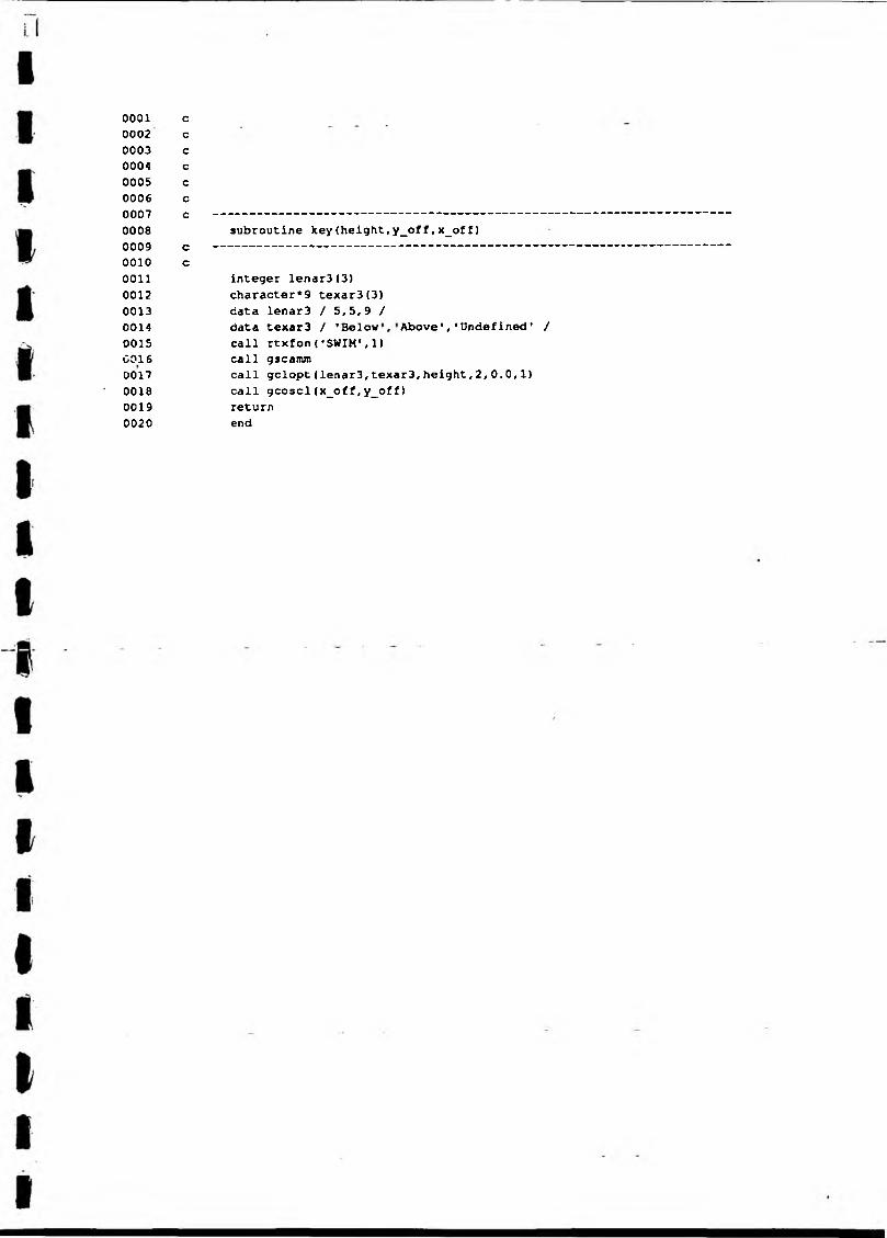
0001 c0002 c0003 c0004 c0005 c0006 c0007 c ------------------------------------------0008 subroutine key(height,y_off,x_off)0009 c -------------------------------------------0010 c0011 integer lenar3(3)0012 character*9 texar3(3)0013 data lenarB / 5,5,9 /0014 data texar3 / ’BelowAbove',1 Undefined * /0015 call rtxfon (* SWIM1,1)0016 call gscamm0017 call gclopt(lenarS,texar3,height, 2,0.0,1)0018 call gcoscl(x_off,y_off)0019 return0020 end

0001 c0002 c0003 c0004 c0005 c0006 c --------------------------------------0007 subroutine raingauge(x,y)0008 c --------------------------------------0009 c0010 include 'quantare.inc’0091 real x(nstat)ry(nstat)0092 c0093 anx<*real (nx)0094 any®real(ny)0095 call glimit(0.0,anx,0.0,any,0.0,0.0)0096 do i-1,nstat0097 call gwells(3, x (i), y (i),1.5,0.02,33)0098 end do0099 return0100 end

Note, that in this example, parameters for 7th August 1989 will be used (other lines commented out).
Appendix 2: Include Flic
mask)
0001 c0002 c0003 c radgap.Inc: an include file used by radgap0004 c0005 c0006 c0007 c PARAMETER NOTES0008 c0009 c ngr_lef_id • ngr coordinates left-side adjustment domain0010 c ngr_rig_id - ngr coordinates right-side adjustment domain001! c ngr_top_id » ngr coordinates of top of adjustment domain0012 c ngr_bot_id • ngr coordinates of bottom of adjustment domain0013 c nx - dimension of interpolation domain (x-axis)0014 c ny - dimension of interpolation domain (y-axis)0015 c xlo - lower bound of interpolation domain (x-axis)0016 c xhi - upper bound of interpolation domain (x-axis)0017 c ylo - lower bound of interpolation domain (y-axis)0018 c yhl - upper bound of interpolation domain (y-axis)0019 c Idom « number of points outside interpolation domain
0020 c start,stop * start and end cells of interpolation domain0021 c nstat - number of raingauge stations0022 c mmax » total number of data points (-nstat+idom)0023 c num_cmt - number of predefined catchments0024 c max_nodes - maximum number of nodes in any catchment0025 c0026 c0027 c0028 c PARAMETER DATA TYPES0029 c0030 integer nx,ny,nstat,idom,max^nodes,num_cmt0031 integer mask_start,mask_stop0032 real xlo,xhi,ylo,yhi,delta,cell0033 real ngr_:lef_id, ngr_rig_id, ngr_top_id, ngr_bot_id0034 c0035 c0036 c PARAMETER STATEMENTS0037 c0038 parameter (cell-5.0)0039 parameter (num_cmt-10,max_nodes-50)0040 parameter {ngr lef_id*4400.0, ngr_rig_id-5700.0)0041 parameter (ngr Jbot_id-2400.0, ngr_top_id*4400.0)0042 c0043 parameter (nx-(ngr_rig_id-ngr_lef_id) / (cell* 10.0) )0044 parameter (ny-(ngr_top_id-ngr_bot_id) / (cell*10.0) )0045 c0046 parameter (xlo-1.0,xhi-real(nx), ylo-1.0,yhi»real(ny))0047 c0048 parameter (idom-522)0049 integer start (ny),stop(ny)0050 c0051 data start / 1, 1, 2, 2, 2, 2, 2, 2, 3, 3,0052 » 3, 4, 5, 6, 7, 7, 7, 1, 7, 7,0053 « 7, 7, 7, 7. 1, 1. 7, 7, 7, 7,0054 1 7, 7, 7, 1, 7, 7, 7, 1, 1, 1 /0055 data stop / 1, 1,11,12,13,14,15,16,16,17,
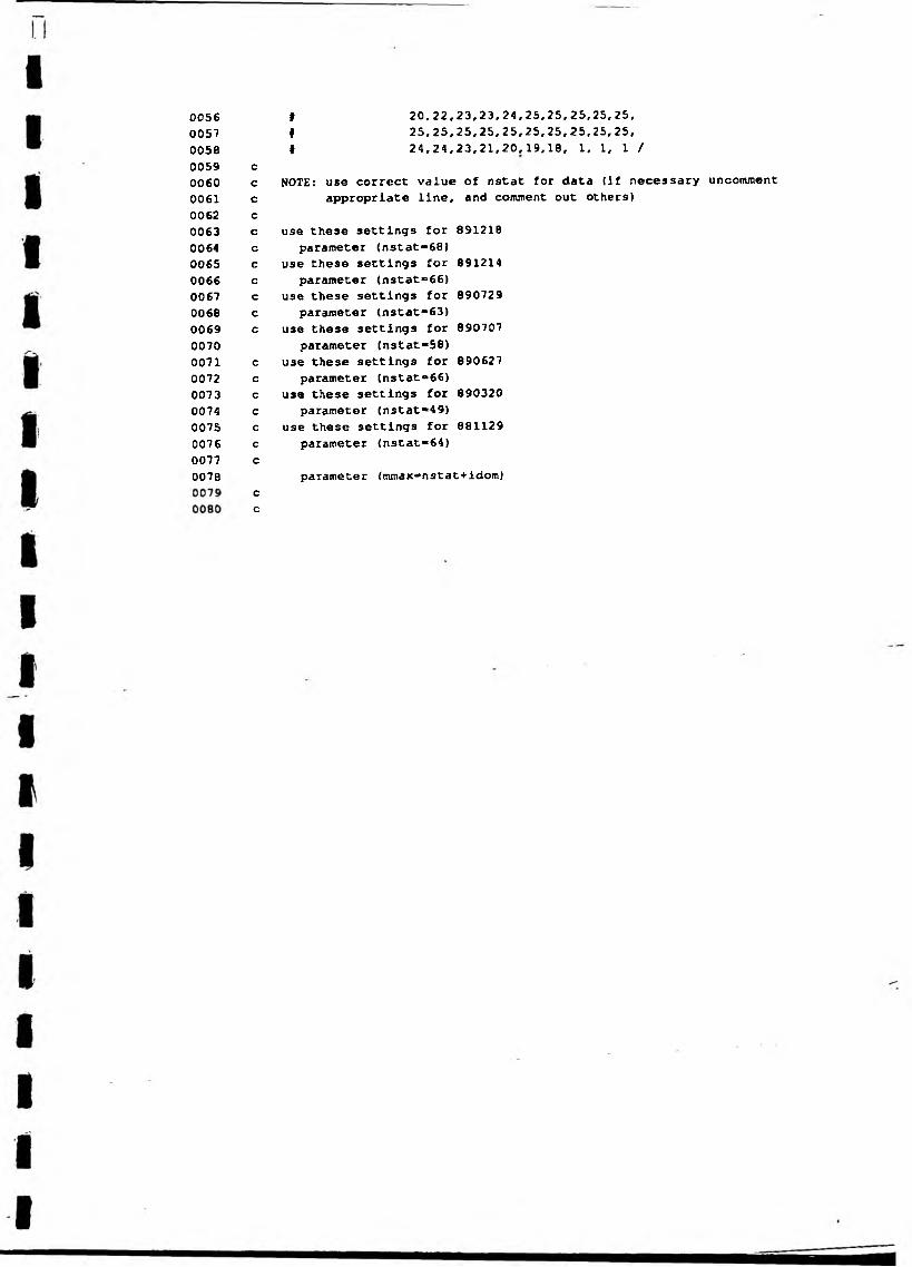
00560057005800590060006100620063006400650066006700680069007000710072007300740075007600770078
# 20,22,23,23,24,25.25,25,25,25,# 25,25,25,25,25,25,25,25,25,25,# 24,24,23,21,20,19,18, 1, 1, 1 /
cc NOTE: use correct value of nstat for data (if necessary uncomment c appropriate line, and comment out others)cc use these settings for 89121B c parameter (nstat-68)c use these settings for 891214 c parameter (nstat**66)c use these settings for 890729 c parameter (nstat-63)c use these settings for 890707
parameter (nstat*58) c use these settings for 890627 c parameter (nstat»66)c use these settings for 890320 c parameter (nstat*49)c use these settings for 881129 c parameter (nstat«64)c
parameter <mmax*nstat+idom)cc
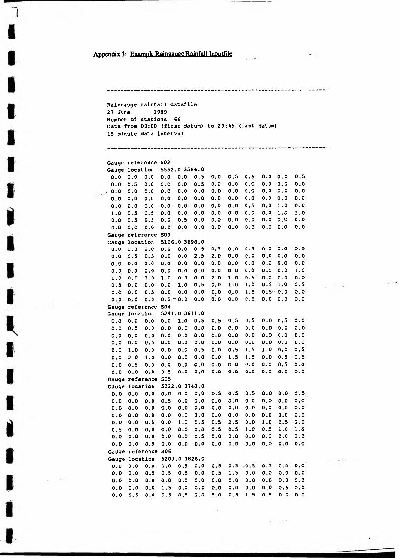
Appendix 3: Example Raingauge Rainfall Inputfile
Raingauge rainfall datafile 27 June 1989Number of stations 66Data from 00:00 (first datum) to 23:45 (last datum)15 minute data interval
Gauge reference 502Gauge location 5552. 0 3586.00.0 0.0 0.0 0.0 0..0 0.5 0.0 0.5 0.5 0.0 0.0 0.0.0 0.5 0.0 0.0 0.,0 0.5 0.0 0.0 0.0 0.0 0.0 0.
. 0.0 0.0 0.0 0.0 0.,0 0.0 0.0 0.0 0.0 0.0 0.0 0.0.0 0.0 0.0 0.0 0.,0 0.0 0.0 0.0 0.0 0.0 0.0 0.0.0 0.0 0.0 0.0 0,.0 0.0 0.0 0.0 0.5 0.0 1.0 0.1.0 0.5 0.5 0.0 0.,0 0.0 0.0 0.0 0.0 0.0 1.0 1,0.0 0.5 0.5 0.0 0..5 0.0 0.0 0.0 0.0 0.0 0.0 0.0.0 0.0 0,0 0.0 0,.0 0.0 0.0 0.0 0.0 0.0 0.0 0.
Gauge reference S03Gauge location 5106,,0 3698.00.0 0.0 0.0 0.0 0..0 0.5 0.5 0.0 0.5 0.0 0.0 0.0.0 0.5 0.5 0.0 0,.0 2.5 2.0 0.0 0.0 0.0 0.0 0.0.0 0.0 0.0 0.0 0,.0 0.0 0.0 0.0 0.0 0.0 0.0 0.0.0 0.0 0.0 0.0 0,.0 0.0 0.0 0.0 0.0 0.0 0.0 1.1.0 0.0 1.0 1.0 0,.0 0.0 2.0 1.0 0.5 0.0 0.0 0.0.5 0.0 0.0 0.0 1,.0 0.5 0.0 1.0 1.0 0.5 1.0 0.0.0 0.0 0.5 0.0 0,.0 0.0 0.0 0,.0 .1.5 0.5 0:0 0.0.0 _ 0.0 0.0 0.5 - 0,.0 0.0 o'.o 0.0 0.0 0.0 0.0 0.
Gauge reference SO AGauge location 5241,,0 3611.00.0 0.0 0.0 0.0 1,.0 0.5 0.5 0.5 0.5 0.0 o.s 0.0.0 0.5 0.0 0.0 0,.0 0.0 0.0 0.0 0.0 0.0 0.0 0.0.0 0.0 0.0 0.0 0.0 0.0 0.0 0.0 0.0 0.0 0.0 0.0.0 0.0 0.5 0.0 0.0 0.0 0.0 0.0 0.0 0.0 0.0 0.0.0 1.0 0.0 0.0 0.0 0.5 0.0 0.5 1.5 1.0 0.0 0.0.0 2.0 1.0 0.0 0.0 0.0 0.0 1.5 1.5 0.0 0.5 0.0.0 0.5 0.0 0.0 0.0 0.0 0.0 0.0 0.0 0.0 0.5 0.0.0 0.0 0.0 0.5 0.0 0.0 0.0 0.0 0.0 0.0 0.0 0.
Gauge reference S05Gauge location 5222..0 3740.00.0 0.0 0.0 0.0 0.0 0.0 0.5 0.5 0.5 0.0 0.0 0.0.0 0.0 0.0 0.5 0.0 0.0 0.0 0.0 0.0 0.0 0.0 0.0.0 0.0 0.0 0.0 0 .0 0.0 0.0 0.0 0.0 0.0 0.0 0.0.0 0.0 0.0 0.0 0 .0 0.0 0.0 0.0 0.0 0.0 0.0 0.0.0 0.0 0.5 0.0 1.0 0.5 0.5 2.5 0.0 1.0 0.5 0.0.5 0.0 0.0 0.0 0 .0 0.0 0.5 0.5 1.0 0.5 1.0 1.0.0 0.0 0.0 0.0 0 .0 0.5 0.0 0.0 0.0 0.0 0.0 0.0.0 0.0 0.5 0.0 0 .0 0.0 0.0 0.0 0.0 0.0 0.0 0.
Gauge reference SO 6Gauge location 5203..0 3826.00.0 0.0 0.0 0.0 0.5 0.0 0.5 0.5 ,0.5 0.5 0:0 0.0.0 0.0 0.5 0.5 0.5 0.0 0.5 1.5 0.0 0.0 0.0 0.0.0 0.0 0.0 0.0 0.0 0.0 0.0 0.0 0.0 0.0 0.0 0.0.0 0.0 0.0 1.5 0.0 0.0 0.0 0.0 0.0 0.0 0.5 0.0.0 0.5 0.0 0.5 0.5 2.0 5.0 0.5 1.5 0.5 0.0 0.
50000000
50000500
00005500
50000000
00000
0.0 0.0 0.0 0.0 0.,0 0.0 0.0 0.5 0.0 2.0 2.0 0.50.0 0.0 0.0 0.0 0..0 0.0 0.5 0.0 0.0 0.0 - 0.0 0.00.0 0.0 0.0 0.5 0..0 0.0 0.0 0.0 0.0 0.0 0.0 0.0
Gauge reference SO 7Gauge location 5296..0 3754.00.0 0.0 0.0 0.0 0..5 0.5 0.0 0.5 0.0 0.5 0.0 0.00.0 0.0 0.0 0.5 0..0 0.0 0.0 0.0 0.0 0.0 0.0 0.00.0 0.0 0.0 0.0 0..0 0.0 0.0 0.0 0.0 0.0 0.0 0.00.0 0.0 0.0 0.0 0,.0 0.0 0.0 0.0 0.0 0.0 0.0 0.00.0 0.0 0.0 0.0 0..0 0.0 0.0 0.5 1.0 0.5 0.0 0.50.0 0.0 0.0 0.0 0,.0 0.0 0.0 0.0 0.0 0.0 0.5 0.50.5 0.0 0.0 0.0 0..0 0.0 0.0 0.0 0.0 0.0 0.0 0.00.0 0.0 0.0 0.0 0..0 0.0 0.0 0.0 0.0 0.0 0.0 0.0
Gauge reference SllGauge location 5319..0 3859.00.0 0.0 0.0 0.0 0,.5 1.0 0.5 0.5 0.0 0.5 0.5 0.00.0 0.0 0.0 0.0 0,.5 0.0 0.0 0.0 0.0 0.0 0.0 0.00.0 0.0 0.0 0.0 0,.0 0.0 0.0 0.0 0.0 0.0 0.0 0.00.0 0.0 0.0 0.0 0,.5 0.0 0.0 0.0 0.0 0.0 0.0 0.00.0 0.0 0.0 0.0 0..0 0.0 0.0 0.0 0.5 1.5 1.5 0.00.5 0.0 0.0 0.0 0..0 0.0 0.0 0.0 0.0 0.0 0.0 1.52.0 1.0 0.0 0.0 0,.0 0.0 0.0 0.0 0.0 0.0 0.0 0.00.0 0.0 0.0 0.0 0,.0 0.0 0.0 0.0 0.0 0.0 0,0 0.0Gauge reference S13Gauge location 4965..0 3756.00.0 0.0 0.0 0.0 0,.0 0.0 0.5 0.0 0.5 0.0 0.0 0.01.0 1.5 0.0 0.0 0..0 0.0 0.0 0.0 0.0 0.0 0.0 0.00.0 0.0 0.0 0.0 0..0 0.0 0.0 0.0 0.0 0.0 0.0 0.00.0 0.0 0.0 0.0 0..0 0.0 0.0 0.0 1.0 1.0 1.0 0.51.0 3.5 1.0 0.0 0,.0 1.0 1.5 1.0 0.5 0.0 0.0 0.00.0 0.5 0.5 0.5 0,.5 0.0 1.0 0.5 0.0 0.0 0.5 0.50.0 0.0 0.0 0.0 0..0 0.0 0.0 0.0 1.0 0.0 0.0 0.00.0 0.0 0.0 0.0 0,.0 0.0 0.0 0.0 0.0 0.0 0.0 0.0
Gauge reference S14 _ -Gauge location_ 5405,.0 3730.0'
o:o 0.0 0.0 0.0 0,.5 o.s 0.5 1.0 0.5 0.5 0.0 0.50.0 0.5 0.0 0.0 0,. 5 0.0 0.0 0.0 0.0 0.0 0.0 0.00.0 0.0 0.0 0.0 0,.0 0.0 0.0 0.0 0.0 0.0 0.0 0.00.0 0.0 0.0 0.0 0,.0 0.0 0.0 0.0 0.0 0.0 0.0 0.00.0 0.0 0.0 0.0 0,.0 0.0 0.0 0.0 0.5 1.0 3.0 0.50.5 0.0 0.0 0.0 0..0 0.0 0.0 0.0 0.5 0.0 0.5 0.51.0 0.5 0.0 0.0 0,.0 0.0 0.0 0.0 0.0 0.0 0.0 0.00.0 0.0 0.5 0.0 0..0 0-0 0.0 0.0 0.0 0.0 0.0 0.0
Gauge reference S16Gauge location 4996 .0 4053.00.0 0.0 0.0 0.0 0,.0 0.0 0.0 0.0 0.0 0.0 0.0 0.00.0 0.0 0.0 0.0 0.0 0.0 0.0 0.0 0.0 0.0 0.0 0.00.0 0.0 0.0 0.0 0.0 0.0 0.0 0.0 0.0 0.0 0.0 0.50.0 0.0 0.5 0.0 0.5 0.0 0.5 0.0 0.0 0.0 0.0 0.00.0 0.0 0.0 0.0 0.0 0.0 0.0 0,0 0.0 0.0 0.0 0.00.0 0.0 0.0 0.0 0.0 0.0 0.0 0.0 0.0 0.0 0.0 0.00.0 0.0 0.0 0.0 0.0 0.0 0.0 0.0 0.0 0.0 0.0 0.00.0 0.0 0.0 0.0 0.0 0.0 0.0 0.0 0.0 0.0 0.0 0.0
Gauge reference S17Gauge location 5174 .0 3356.00.0 0.0 0.0 0.0 0.5 0.5 0.5 0.0 0.5 0.5 0.5 0.00.0 1.5 0.0 0.0 0.0 0.0 0.0 0.0 0.0 0.0 0.0 0.00.0 0.0 0.0 0.0 0.0 0.0 0.0 0.0 0.0 0.0 = 0.0 0.00.0 0.0 0.0 0.0 0.0 0.0 0.0 0.0 0.0 0.0 0.0 0.00.0 0.0 0.0 0.0 0.0 0.0 0.0 0.0 0.0 0.0 0.0 0.00.5 0.5 0.5 1.0 0.5 1.0 1.0 0.5 0.5 0.0 0.0 0.00.0 0.0 1.0 0.0 0.0 0.0 0.0 0.0 0.0 0.0 0.0 0.0

0.5 0.0 0.0 0.0 0.0 0.0 0.0 0.0 0.0 0.0 0.0 0.0Gauge reference s i eGauge location 5324. 0 3445.00.0 0.0 0.0 0.0 0.5 0.5 0.5 0.5 0.0 0.5 0.5 0.00.0 0.0 0.5 0.0 0.0 0.0 0.0 0.0 0.0 0.0 0.0 0.00.0 0.0 0.0 0.0 0.0 0.0 0.0 0.0 0.0 0.0 0.0 0.00.0 0.0 0.0 0.0 0.0 0.0 0.0 0.0 0.0 0.0 0.0 0.00.0 0.0 0.5 0.0 0.0 0.0 0.0 0.0 0.0 0.0 0.5 1.00.0 0.5 0.0 0.0 0.0 0.0 0.0 0.5 0.0 1.0 0.0 0.00.0 0.0 0.0 0.0 0.0 0.0 0.0 0.0 0.0 0.0 0.0 0.00.0 0.0 0.0 0.0 0.0 0.0 0.0 0.0 0.0 0.0 0.0 0.0
Gauge reference T01Gauge location 4661.,0 2831.00.0 0.0 0.0 0.0 0.0 0.0 o-.o 0.0 1.5 1.5 0.0 0.00.0 0.0 0.0 0.0 0.0 0.0 0.0 0.0 0.0 0.0 0.0 0.00.0 0.0 0.0 0.0 0.0 0.0 0.0 0.0 0.0 0.0 0.0 0.00.0 0.0 0.0 0.0 3.5 1.0 0.5 0.5 0.0 0.0 0.0 0.00.0 0.0 0.0 0.0 0.0 0.0 0.0 0.0 0.0 0.0 0.0 0.00.0 0.0 0.0 0.0 0.0 0.0 0.0 0.0 0.0 0.0 0.0 0.00.0 0.0 0.0 0.0 0.0 0.0 0.0 0.0 0.0 0.0 0.0 0.00.0 0.0 0.0 0.0 0.0 0.0 0.0 0.0 0.0 0.0 0.0 0.0
Gauge reference T02Gauge location 4638,.0 3065.00.0 0.0 0.0 0.0 0.5 0.5 0.0 0.0 0.5 0.5 0.5 0.50.5 0.0 0.0 0.0 0.0 0.0 0.0 0.0 0.0 0.0 0.0 0.00.0 0.0 0.0 0.0 0.0 0.0 0.0 0.0 0.0 0.0 0.0 0.00.0 0.0 0.0 0.5 0.0 0.0 0.0 0.0 0.0 0.0 0.0 0.00.0 0.0 0.0 0.0 0.0 0.0 0.5 0.0 0.0 0.0 0.0 0.00.0 0.0 0.0 0.0 0.0 0.0 0.0 0.0 0.0 0.0 0.0 0.00.0 0.0 0.0 0.0 0.0 0.0 0.0 0.0 0.0 0.0 0.0 0.00.0 0.0 0.0 0.0 0 .0 0 .0 0.0 0.0 0.0 0.0 0.0 0.0
Gauge reference T03Gauge location 5124,.0 2982.00.0' 0.0 0. 0 0.0 0 .0 0.0 0.0 0.0 0.0 0.5 0.0 1.00.5 0.5 0.0 0.0 0.0 0 .0 0.0 0.0 0.0 0.0 0.0 0.00.0 0.0 0.0 0.0 0 .0 0.0 0.0 0.0 0.0 0.0 0.0 0.00.0 0.0 0.0 0.0 2.5 0.5 0.0 0.0 0.0 0.0 0.0 0.00.0 0.0 0.0 0.0 0 .0 0.0 0.0 0.0 0.0 0.5 0.5 0.50 .0 0.0 0.0 0.0 0.0 0.0 0.0 0.0 0.0 0.0 0.0 0.00.0 0.0 0.0 0.0 0.0 0.0 0.0 0.0 0.0 0.0 0.0 0.00.0 0.0 0.0 0.0 0.0 0.0 0.0 0.0 0.0 0.0 0.0 0.0
Gauge reference T0SGauge location 4627 .0 2607.00.0 0.0 0.0 0.0 0.0 0.0 0.0 0.0 0.0 0.0 0.0 0.00.5 0.0 0.0 0.0 0.0 0.0 0.0 0.0 0.0 0.0 0.0 0.00.0 0.0 0.0 0.0 0 .0 0.0 0.0 0.0 0.0 0.0 0.0 0.00.0 0.0 0.0 0.0 0.0 0.5 0.0 0.0 0.0 0.0 0.0 0.00.0 0.0 0.5 0.0 0.0 0.0 0.0 0.5 0.0 0.0 0.0 0.00.0 0.0 0.0 0.0 0.0 0.0 0.0 0.0 0.0 0.0 0.0 0.00.0 0.0 0.0 0.0 0.0 0.0 0.0 0.0 0.0 0.0 0.0 0.00.0 0.0 0.0 0.0 0.0 0.0 0.0 0.0 0.0 0.0 0.0 0.0
Gauge reference T07Gauge location 5013 .0 2975.00.0 0.0 0.0 0.0 0.0 0.5 0.0 0.0 0.0 0.0 1.0 1.50.0 0.0 0.0 0.0 0.0 0.0 0.0 0.0 0.0 0.0 0.0 0.00.0 0.0 0.0 0.0 0.0 0.0 0.0 0.0 0.0 0.0 0.0 0.00.0 0.0 0.5 1.5 0.5 0.0 0.5 0.0 0.0 0.0 0.0 0.00.0 0.0 0.0 0.0 0.0 0.0 0.0 0.0 0.0 0.5 0.0 0.00.0 0.0 0.0 0.0 0.0 0.0 0.0 0.0 0.0 0.0 0.0 0.00.0 0.0 0.0 0.0 0.0 0.0 0.0 0.0 0.0 0.0 0.0 0.00.0 0.0 0.0 0.0 0.0 0.0 0.0 0.0 0.0 0.0 0.0 0.0Gauge reference T10
Gauge location 4867.,0 2574.0 _0.0 0.0 0.0 0.0 0.0 0.0 0.0 0.0 0.0 0.5 0.0 0.00.0 0.0 0.0 0.0 0.0 0.0 0.0 0.0 0.0 0.0 0.0 0.00.0 0.0 0.0 0.0 0.0 0.0 0.0 0.0 0.0 0.0 0.0 0.00.0 0.0 0.0 0.0 0.0 0.0 0.5 0.5 0.0 0.0 0.0 0.00.0 0.0 0.0 0.0 0.0 0.0 0.0 0.0 0.0 0.0 0.0 0.00.0 0.0 0.0 0.0 0.0 0.0 0.0 0.0 0.0 0.0 0.0 0.00.0 0.0 0.0 0.0 0.0 0.0 0.0 0.0 0.0 0.0 0.0 0.00.0 0.0 0.0 0.0 0.0 0.0 0.0 0.0 0.0 0.0 0.0 0.0Gauge reference U01Gauge location 5109,,0 3202.00.0 0.0 0.0 0.0 0.5 0.5 0.5 0.5 0.0 0.0 0.0 0.01.5 0.5 0.0 0.0 0.0 0.0 0.0 0.0 0.0 0.0 0.0 0.00.0 0.0 0.0 0.0 0.0 0.0 0.0 0.0 0.0 0.0 0.0 0.00.0 0.0 0.0 0.0 0.0 0.0 0.0 0.0 0.5 0.0 0.0 0.00.0 0.0 0.0 1.5 1.0 0.0 0.0 0.0 0.0 0.0 0.5 0.50.0 0.0 0.0 0.0 0.0 1.5 1.0 0.5 0.0 0.0 0.0 0.00.0 0.0 0.0 0.0 0.0 0.0 0.0 0.0 0.0 0.0 0.0 0.00.0 0.0 0.0 0.0 0.0 0.0 0.0 0.0 0.0 0.0 0.0 0.0Gauge reference U04Gauge location 4992 .0 3247.00.0 0.0 0.0 0.0 0.5 0.5 0.0 0.5 0.5 0.0 0.0 0.00.5 0.0 0.0 0.0 0.0 0.0 0.0 0.0 0.0 0.0 0.0 0.00.0 0.0 0.0 0.0 0.0 0.0 0.0 0.0 0.0 0.0 0.0 0.00.0 0.0 0.0 0.0 0.0 0.0 0.0 0.0 0.0 0.0 0.0 0.00.0 0.0 1.0 1.5 0.5 0.0 0.0 0.5 0.5 0.5 0.5 1.00.0 0.0 0.0 0.0 0.0 0.0 0.0 0.0 0.0 0.0 0.0 0.00.0 0.0 0.0 0.0 0.0 0.0 0.0 0.0 0.0 0.0 0.0 0.00.0 0.0 0.0 0.0 0.0 0.0 0.0 0.0 0.0 0.0 0.0 0.0Gauge reference 005Gauge location 5246.0 3091.00.0 0.0 0.0 0.0 0.5 0.0 0.5 0.0 0.0 0.0 0.0 0.00.5 1.0 0.0 0.0 0.0 0.0 0.0 0.0 0.0 0.0 0.0 0.00.0 0.~0 o:o 0.0 0.0 0.0 0.0 0.0 0.0 oro o:o 0.00.0 0.0 0.0 0.0 2.5 0.5 0.5 0.0 0.0 0.0 0.0 0.00.0 0.0 0.0 0.0 0.0 0.5 0.0 0.0 0.0 0.0 0.0 0.50.0 0.0 0.0 0.5 0.0 0.0 2.0 1.0 0.5 0.0 0.0 0.00.0 0.0 0.0 0.0 0.0 0.0 0.0 0.0 0.0 0.0 0.0 0.00.0 0.0 0.0 0.0 0.0 0.0 0.0 0.0 0.0 0.0 0.0 0.0Gauge reference 006Gauge location 5272 .0 3993.00.0 0.0 0.0 0.0 0.5 0.0 0.0 0.0 0.0 0.0 0.0 0.00.5 0.0 0.0 0.0 0.0 0.0 0.0 0.0 0.0 0.0 0.0 0.00.0 0.0 0.0 0.0 0.0 0.0 0.0 0.0 0.0 0.0 0.0 0.00.0 0.0 0.0 0.0 0.0 0.0 0.0 0.5 0.0 0.5 0.0 0.00.0 0.0 0.0 0.0 0.0 0.0 0.0 0.0 0.0 0.0 0.0 0.50.0 0.0 0.5 0.0 0.0 0.0 0.0 2.0 1.0 0.0 0.0 0.00.0 0.0 0.0 0.0 0.0 0.0 0.0 0.0 0.0 0.0 0.0 0.00.0 0.0 0.0 0.0 0.0 0.0 0.0 0.0 0.0 0.0 0.0 0.0Gauge reference U07Gauge location 5143 .0 3051.00.0 0.0 0.0 0.0 0.0 0.5 0.0 0.0 0.0 0.0 0.5 1.50.0 0.5 0.5 0.0 0.0 0.0 0.0 0.0 0.0 0.0 0.0 0.00.0 0.0 0.0 0.0 0.0 0.0 0.0 0.0 0.0 0.0 0.0 0.00.0 0.0 0.0 0.5 0.5 0.0 0.0 0.0 0.0 0.0 0.0 0.00.0 0.0 0.0 0.0 0.0 0.0 0.0 0.0 0.0 0.5 0.0 0.00.5 0.0 0.0 0.0 0.0 0.0 0.5 0.0 0.0 0.0 0.0 0.00.0 0.0 0.0 0.0 0.0 0.0 0.0 0.0 0.0 0/0 0.0 0.00.0 0.0 0.0 0.0 0.0 0.0 0.0 0.0 0.0 0.0 0.0 0.0
Gauge reference U08Gauge location 5177 .0 3008.00.0 0.0 0.0 0.0 0.5 0.0 0.0 0.0 0.0 0.0 0.0 0.5

1.0 0.0 0.0 0.0 0,.0 0.0 0.0 0.0 0.0 0.0 0.0 0.00.0 0.0 0.0 0.0 0..0 0.0 0.0 0.0 0.0 0.0 0.0 0.00.0 0.0 0.0 0.0 6..0 0.0 0.5 0.0 0.0 0.0 0.0 0.00.0 0.0 0.0 0.0 0.0 0.0 0.0 0.0 0.0 0.0 0.5 0.00.0 0.5 0.5 0.0 0,.0 0.0 0.0 0.0 0.0 0.0 0.0 0.00.0 0.0 0.0 0.0 0,.0 0.0 0.0 0.0 0.0 0.0 0.0 0.00.0 0.0 0.0 0.0 0,.0 0.0 0.0 0.0 0.0 0.0 0.0 0.0Gauge reference 010Gauge location 5358.,0 3258.00.0 0.0 0.0 0.0 0,.5 0.5 0.5 0.0 0.0 0.0 0.5 0.00.0 0.5 0.5 0.5 0,.5 0.5 0.0 0.0 0.0 0.0 0.0 0.00.0 0.0 0.0 0.0 0,.0 0.0 0.0 0.0 0.0 0.0 0.0 0.00.0 0.0 0.0 0.5 0,.0 0.0 0.0 0.0 0.0 0.0 0.0 0.00.0 0.0 0.0 0.0 0,.0 0.0 0.0 0.0 0.0 0.0 0.0 0.00.0 0.5 0.5 0.0 0,.0 0.0 0.5 0.5 1.0 0.5 0.0 0.00.0 0.0 0.0 0.0 0,.5 0.0 0.0 0.0 0.0 0.0 0.0 0.00.0 0.0 0.0 0.0 0.0 0.0 0.0 0.0 0.0 0.0 0.0 0.0
Gauge reference OilGauge location 5067,.0 3164.00.0 0.0 0.0 0.0 0.5 0.0 0.5 0.0 0.5 0.5 0.5 0.00.0 0.0 0.0 2.0 0,,5 0.0 0.5 0.0 0.0 0.0 0.0 0.00.0 0.0 0.0 0.0 0,.0 0.0 0.0 0.0 0.0 0.0 0.0 0.00.0 0.0 0.0 0.0 0.0 0.0 0.0 0.0 0.0 0.0 0.0 0.00.0 0.0 0.0 0.0 0,.0 0.0 0.5 0.0 0.0 0.0 0.0 0.00.0 0.5 0.0 0.0 0,.5 0.0 0.0 0.0 0.0 0.0 0.0 0.00.0 0.0 0.0 0.0 0,.0 0.0 0.0 0.0 0.0 0.0 0.0 0.00.0 0.0 0.0 0.0 0,.0 0.0 0.0 0.0 0.0 0.0 0.0 0.0Gauge reference U13Gauge location 5201 .0 2984.00.0 0.0 0.0 0.0 0.0 0.5 0.0 0.0 0.0 0.0 0.0 0.00.5 0.0 0.0 0.0 0.0 0.0 0.0 0.0 0.0 0.0 0.0 0.00.0 0.0 0.0 0.0 0,.0 0.0 0.0 0.0 0.0 0.0 0.0 0.00.0 0.0 0.0 0.0 0,.0 0.0 0.5 0.0 0.0 0.0 0.0 0.00.0 0.0̂ 0.0 0,0 0.0- 0.0 0.0 0.0 0.0 -o.o 0.5 0.00.0 0.5 0.0 0.0 0.0 0.0 0.0 0.5 0.0 0.0 0.0 0.00.0 0.0 0.0 0.0 0.0 0.0 0.0 0.0 0.0 0.0 0.0 0.00.0 0.0 0.0 0.0 0.0 0.0 0.0 0.0 0.0 0.0 0.0 0.0Gauge reference U14Gauge location 5201,.0 3003.00.0 0.0 0.0 0.0 0.0 0.0 0.0 0.0 0.0 0.0 0.0 0.50.0 0.0 0.0 0.5 0.0 0.0 0.0 0.0 0.0 0.0 0.0 0.00.0 0.0 0.0 0.0 0.0 0.0 0.0 0.0 0.0 0.0 0.0 0.00.0 0.0 0.0 0.0 3.5 3.5 0.0 0.0 0.5 0.0 0.0 0.00.0 0.0 0.0 0.0 0.0 0.0 0.0 0.0 0.0 0.0 0.0 0.50.0 0.5 0.5 0.0 0.0 0.0 0.0 0.5 0.0 0.0 0.0 0.00.0 0.0 0.0 0.0 0.0 0.0 0.0 0.0 0.0 0.0 0.0 0.00.0 0.0 0.0 0.0 0.0 0.0 0.0 0.0 0.0 0.0 0.0 0.0Gauge reference 015Gauge location 5193 .0 2986.00.0 0.0 0.0 0.0 0.0 0.5 0.0 0.0 0.0 0.0 0.0 0.00.5 0.0 0.0 0.0 0.0 0.0 0.0 0.0 0.0 0.0 0.0 0.00.0 0.0 0.0 0.0 0.0 0.0 0.0 0.0 0.0 0.0 0.0 0.00.0 0.0 0.0 0.0 1.5 1.0 0.5 0.0 0.0 0.0 0.0 0.00.0 0.0 0.0 0.0 0.0 0.0 0.0 0.0 0.0 0.0 0.0 0.50.0 0.5 0.5 0.0 0.0 0.0 0.0 0.0 0.0 0.0 0.0 0.00.0 0.0 0.0 0.0 0.0 0.0 0.0 0.0 0.0 0.0 0.0 0.00.0 0.0 0.0 0.0 0.0 0.0 0.0 0.0 0.0 0.0 0.0 0.0Gauge reference 017 —
Gauge location 5001 .0 3336.00.0 0.0 0.0 0.0 0.5 0.5 0.0 0.5 0.0 0.5 0.0 0.00.5 0.5 0.0 0.5 0.0 0.0 0.0 0.0 0.0 0.0 0.0 0.00.0 0.0 0.0 0.0 0.0 0.0 0.0 0.0 0.0 0.0 0.0 0.0

0.0 0.0 0.0 0.0 0.0 0.0 0.0 0.0 0.0 0.0 0.0 0.00.0 0.0 0.0 0.5 0.0 0.0 0.0 0.5 0.5 0.5 1.0 0.00.5 0.0 0.0 0.0 4.0 2.0 0.0 0.0 0.0 0.0 0.0 0.00.0 0.0 0.0 0.0 0.0 0.0 0.0 0.0 0.0 0.0 0.0 0.50.0 0.0 0.0 0.0 0.0 0.0 0.0 0.0 0.0 0.0 0.0 0.0
Gauge reference U18Gauge location 4946.0 3081.00.0 0.0 0.0 0.0 0.5 0.5 0.5 0.0 0.5 0.0 0.5 0.50.5 0.0 1.0 0.0 0.0 0.0 0.0 0.0 0.0 0.5 0.0 0.00.0 0.0 0.0 0.0 0.0 0.0 0.0 0.0 0.0 0.0 0.0 0.00.0 0.0 0.0 0.0 0.0 0.0 0.0 0.0 0.0 0.0 0.0 0.00.0 0.0 1.5 1.0 0.5 0.0 0.0 0.5 0,5 0.5 1.0 0.00.5 0.0 0.0 0.0 0.0 0.0 0.0 0.0 0.0 0.0 0.0 0.00.0 0.0 0.0 0.0 0.0 0.0 0.0 0.0 0.0 0.0 0.0 0.00.0 0.0 0.0 0.0 0.0 0.0 0.0 0.0 0.0 0.0 0.0 0.0
Gauge reference U19Gauge location 5262..0 3251.00.0 0.0 0.0 0.0 0.5 0.0 0.5 0.5 0.0 0.5 0.0 0.00.5 1.5 0.0 0.0 0.0 0.0 0.0 0.0 0.0 0.0 0.0 0.00.0 0.0 0.0 0.0 0.0 0.0 0.0 0.0 0.0 0.0 0.0 0.00.0 0.0 0.0 0.0 0.0 0.0 0.0 0.0 0.0 0.0 0.0 0.00.0 0.0 0.0 0.0 0.0 0.0 0.0 0.0 0.0 0.5 0.0 0.00.0 0.5 0.0 1.5 1.0 0.5 0.5 1.0 0,5 0.0 0.0 0.00.0 0.0 0.0 0.0 0.0 0.0 0.0 0.0 0.0 0.0 0.0 0.00.0 0.0 0.0 0.0 0.0 0.0 0.0 0,0 0.0 0.0 0.0 0.0
Gauge reference 021Gauge location 5476,.0 3201.00.0 0.0 0.0 0.0 0.5 0.0 0,5 0.0 0.5 0.0 0.0 0.00.0 0.0 0.5 0.0 0.0 0,0 0.0 0.0 0.0 0.0 0.0 0.00.0 0.0 0.0 0.0 0.0 0.0 0.0 0.0 0.0 0.0 0.0 0.00.0 0.0 0.0 0.0 0.0 0.0 0.5 0.0 0.5 0.5 0.0 0.00.0 0.0 0.0 0.0 0.0 0.0 0.5 0.0 0.0 0.0 0.0 0.50.0 0.5 0.0 0.0 0.5 0.0 0.0 0.5 0.0 0.5 0.5 0.00.0 0.0 0.0 0.0 0.0 0.0 0.0 0.0 0.0 0.0 0.0 0.00.0 0.5 0.0 0.0 ~0.0“ “o7o o7o "oro ~o:o~ 0 70' O'.O 0.0
Gauge reference U22Gauge location 5183,.0 3029.00.0 0.0 0.0 0.0 1.0 0.0 0.5 0.0 0.5 0.0 0.0 0.00.0 0.0 0.5 1.5 0.0 0.5 0.0 0.0 0.0 0.0 0.0 0.00.0 0.0 0.0 0.0 0.0 0.0 0.0 0.0 0.0 0.0 0.0 0.00.0 0.0 0.0 0.0 0.0 0.0 0.5 1.5 0.5 0.0 0.0 0.50.0 0.0 0.0 0.0 0.0 0.0 0.0 0.0 0.0 0.0 0.0 0.00.0 0.0 0.5 0.0 0.0 0.0 0.0 0.0 0.0 0.0 1.0 0.00.0 0.0 0.0 0.0 0.0 0.0 0.0 0.0 0.0 0.0 0.0 0.00.0 0.0 0.0 0.0 0.0 0.0 0.0 0.0 0.0 0.0 0.0 0.0
Gauge reference U23Gauge location 5460.0 3140.00.0 0.0 0.0 0.0 0.0 0.5 0.0 0.5 0.0 0.5 0.0 0.00.0 0.0 0.0 0.0 0.5 0.0 0.0 0.0 0.0 0.0 0.0 0.00.0 0.0 0.0 0.0 0.0 0.0 0.0 0.0 0.0 0.0 0.0 0.00.0 0.0 0.0 0.0 0.0 0.0 0.0 0.5 0.5 0.0 0.0 0.00.0 0.0 0.0 0.0 0.0 0.5 0.5 0.0 0.0 0.0 0.0 0.50.0 0.0 0.5 1.0 0.0 0.0 0.0 1.0 1.5 1.0 0.0 0.00.0 0.0 0.0 0.0 0.0 0.0 0.0 0.0 0.0 0.0 0,0- 0.00.0 0.0 0.5 0.0 0.0 0.0 0.0 0.0 0.0 0.0 0.0 0.0
Gauge reference 025Gauge location 5274 .0 3962.00.0 0.0 0.0 0.0J 0.5 0.0 0.0 0.0 0.0 0.0 0.0 0.50.0 0.0 0.0 0.0 J 0.0 0.0 0.0 “ 0.0 0.0 0.0 0.0 "0.00.0 0.0 0.0 0.0 0.0 0.0 0.0 0.0 0.0 0.0 0.0 0.00.0 0.0 0.0 0.0 0.0 0.0 0.0 0.5 0.5 0.0 0.0 0.00.0 0.0 0.0 0.0 0.0 0.0 0.0 0.0 0.0 0.0 0.5 0.0

0.0 0.0 1.5 0.0 0 . 0 0.0 0.0 0.5 0.5 0.0 0.0 0.00.0 0.0 0.0 0.0 0 . 0 0.0 0 .0 0.0 0.0 0-0. 0.0 0.00.0 0.0 0.0 0.0 0 . 0 0.0 0 .0 0.0 0.0 0.0 0.0 0.0
Gauge reference V01Gauge location 4760.0 2647.00.0 0.0 0.0 0.0 0.0 0.0 0.0 0.0 2.5 0.5 0.5 0.00.0 0.0 0.0 0.0 0 . 0 0.0 0 . 0 0.0 0.0 0.0 0.0 0.00.0 0.0 0.0 0.0 0 . 0 0.0 0.0 0.0 0.0 0.0 0.0 0.00.0 0.0 1.0 1.0 1 . 5 1.0 0.5 0.0 0.0 0.0 0.0 0.00.0 0.0 0.0 0.0 0 . 0 0.0 0.0 0.0 0.0 0.0 0.0 0.00.0 0.0 0.0 0.0 0.0 0.0 0.0 0.0 0.0 0.0 0.0 0.00.0 0.0 0.0 0.0 0 . 0 0.0 0 .0 0.0 0.0 0.0 0.0 0.00.0 0.0 0.0 0.0 0 . 0 0.0 0.0 0.0 0.0 0.0 0.0 0.0
Gauge reference V02Gauge location 4902. 0 2593.00.0 0.0 0.0 0.0 0 .,0 0.0 0 .0 0.0 0.0 0.5 0.0 2.00.0 0.0 0.0 0.0 0.0 0.0 0.0 0.0 0.0 0.0 0.0 0.00.0 0.0 0.0 0.0 0..0 0.0 0 .0 0.0 0.0 0.0 0.0 0.00.0 0.0 0.0 2.0 1 ..0 0.0 0.0 0.5 0.0 0.0 0.0 0.00.0 0.0 0.0 0.0 0 .,0 0.0 0.0 0.0 0.0 0.0 0.0 0.00.0 0.0 0.0 0.0 0 .,0 0.0 0.0 0.0 0.0 0.0 0.0 0.00.0 0.0 0.0 0.0 0 . 0 0.0 0 .0 0.0 0.0 0.0 0.0 0.00.0 0.0 0.0 0.0 0 ..0 0.0 0 .0 0.0 0.0 0.0 0,0 0.0Gauge reference V03Gauge location 4946..0 2847.00.0 0.0 0.0 0.0 0.>0 0.0 0.0 0.0 0.0 1.5 1.0 1.50.0 0.0 0.0 0.0 0 .,0 0.0 0 .0 0.0 0.0 0.0 0.0 0.00.0 0.0 0.0 0.0 0..0 0.0 0.0 0.0 0.0 0.0 0.0 0.00.0 0.0 0.0 4.5 1.,5 2.5 0.5 0.0 0.5 0.0 0.0 0.00.0 0.0 0.0 0.0 0 .,0 0.0 0.0 0.0 0.0 0.0 0.0 0.00.0 0.0 0 .0 0.0 0.,0 0.0 0.0 0.0 0.0 0.0 0.0 0.00.0 0.0 0.0 0.0 0..0 0.0 0.0 0.0 0.0 0.0 0.0 0.00.0 0.0 0.0 0.0 0 ..0 0.0 0.0 0.0 0.0 0.0 0.0 0.0
Gauge reference V04Gauge location 5000'.0 3024.0 - - - -0.0 0.0 0.0 0.0 0,.0 1.0 0.0 0.0 0.0 0.5 2.0 0.50.0 0.0 0.0 0.0 0 ..0 0.0 0.0 0.0 0.0 0.0 0.0 0.00.0 0.0 0.0 0.0 0..0 0.0 0.0 0.0 0.0 0.0 0.0 0.00.5 0.0 0.0 0.5 0 ,.0 0.0 0.0 0.0 0.0 0.0 0.0 0.00.0 0.0 0.0 0.0 0 ..0 0.0 0.5 0.5 o.s 1.0 0.0 0.50.0 0.0 0.0 0.0 0,.0 0.0 0.0 0.0 0.0 0.0 0.0 0.00.0 0.0 0.0 0.0 0 ..0 0.0 0.0 0.0 0.0 0.0 0.0 0.00.0 0.0 0.0 0.0 0 ,.0 0.0 0.0 0.0 0.0 0.0 0.0 0.0Gauge reference V05Gauge location 4861 .0 2686.00.0 0.0 0.0 0.0 0,.5 0.0 0.5 0.0 0.0 0.0 0.0 0.00.0 0.0 0.5 0.0 0,.0 0.0 0.0 0.0 0.0 0.0 0.5 0.00.0 0.0 0.0 0.0 0 ,.0 o.s 0.0 0.0 0.0 0.0 0.0 0.50.0 0.0 0.0 0.0 0 ,.0 0.0 0.0 0.5 0.0 0.0 0.0 0.00.0 0.0 0 .0 0.0 0 ,.S 0.0 0.0 0.0 0.0 0.0 0.0 0.00.0 0.5 0.0 0.0 0 .0 0.0 0.0 0.0 0.0 0.0 0.5 0.00.0 0.0 0 .0 0.0 0 ,.0 0.0 0.0 0.0 0.0 0.0 0.0 0.00.0 0.0 0.0 0.0 0 ,.0 0.0 0.0 0.0 0.0 0.0 0.0 0.0Gauge reference V0 6Gauge location 5148..0 2946.00.0 0.0 0.0 0.0 0,.0 0.0 0.0 0.0 0.0 0.0 0.5 0.50.0 0.5 0.0 0.0 0.0 0.0 0.0 0.0 0.0 0.0 0.0 0.00.0 0.0 0.0 0.0 0 ,.0 0.0 0.0 0.0 0.0 0.0 0.0 0.00.0 0.0 0.0 0.0 0.0 1.0 0.0 0.0 0.0 0.5 0.0 0.00.0 0.0 0.0 0.0 0.0 0.0 0.0 0.0 0.0 0.5 1.0 1.00.0 0.0 0.0 0.0 0.0 0.0 0.0 0.0 0.0 0.0 0.0 0 . 00.0 0.0 0.0 0.0 0.0 0.0 0.0 0.0 0.0 0.0 0.0 0.0

0.0 0.0 0.0 0.0 0.0 0.0 0.0 0.0 0.0 0.0 0.0 0.0Gauge reference V0 7Gauge location 4584 .0 2619.00.0 0.0 0.0 1.0 0.0 0.0 2.5 1.5 0.0 0.0 0.0 0.00.0 0.0 0.0 0.0 0.0 0.0 0.0 0.0 0.0 0.0 0.0 0.50.0 0.0 0.0 0.0 0.0 0.0 0.0 0.0 0.0 0.0 0.0 0.00.0 0.0 0.0 0.0 0.5 0.5 0.0 0.0 0.0 0.0 0.0 0.00.0 0.0 0.0 0.0 0.0 0.5 0.0 0.0 0.0 0.0 0.0 0.00.0 0.0 0.0 0.0 0.,0 0.0 0.0 0.0 0.0 0.0 0.0 0.00.0 0.0 0.0 0.0 0.0 0.0 0.0 0.0 0.0 0.0 0.0 0.00.0 0.0 0.0 0.0 0.0 0.0 0.0 0.0 0.0 0.0 0.0 0.0
Gauge reference V0 8Gauge location 4774..0 2867.00.0 0.0 0.0 0.0 0.5 0.0 0.0 0.0 1.5 3.5 0.5 0.00.0 0.0 0.0 0.0 0,.0 0.0 0.0 0.0 0.0 0.0 0.0 0.00.0 0.0 0.0 0.0 0.0 0.0 0.0 0.0 0.0 0.0 0.0 0.00.0 0.$ 4.5 1.0 0..5 0.5 0.0 0.5 0.0 0.0 0.0 0.00.0 0.0 0.0 0.0 0.0 0.0 0.0 0.0 0.0 0.0 0.0 0.00.0 0.0 0.0 0.0 0..0 0.0 0.0 0.0 0.0 0.0 0.0 0.00.0 0.0 0.0 0.0 0.0 0.0 0.0 0.0 0.0 0.0 0.0 0.00.0 0.0 0.0 0.0 0.,0 0.0 0.0 0.0 0.0 0.0 0.0 0.0Gauge reference VO 9Gauge location 4754..0 2768.00.0 0.0 0.0 0.0 0.,0 0.0 0.0 0.5 2.5 0.5 0.5 0.00.0 0.0 0.0 0.0 0..0 0.0 0.0 0.0 0.0 0.0 0.0 0.00.0 0.0 0.0 0.0 0.,0 0.0 0.0 0.0 0.0 0.0 0.0 0.00.0 0.0 0.0 0.0 0..5 0.5 0.5 0.0 0.0 0.0 0.0 0.00.0 0.0 0.0 0.0 0..0 0.0 0.0 0.0 0.0 0.0 0.0 0.00.0 0.0 0.0 0.0 0.,0 0.0 0.0 0.0 0.0 0.0 0.0 0.00.0 0.0 0.0 0.0 0.,0 0.0 0.0 0.0 0.0 0.0 0.0 0.00.0 0.0 0.0 0.0 0..0 0.0 0.0 0.0 0.0 0.0 0.0 0.0
Gauge reference VI0Gauge location 4729,.0 2596.00.0 0.0 0.0 0.0 0..0 0.0 0.0 0.5 0.5 0.0 0.5 0.00.0 0.0 _ 0.0 0.0 -■O'..0 0.0 0.0 0.0 o.o‘ 0.0 0.0 0.00.0 0.0 0.0 0.0 0.,0 0.0 0.0 0.0 0.0 0.0 0.0 0.00.0 0.0 0.0 0.0 0,.0 0.0 0.5 0.0 0.0 0.0 0.0 0.00.0 0.0 0.0 0.5 0..0 0.0 0.5 0.0 0.0 0.0 0.0 0.00.0 0.0 0.0 0.0 0,.0 0.0 0.0 0.0 0.0 0.0 0,0 0.00.0 0.0 0.0 0.0 0,.0 0.0 0.0 0.0 0.0 0.0 0.0 0.00.0 0.0 0.0 0.0 0,.0 0.0 0.0 0.0 0.0 0.0 0.0 0.0Gauge reference VI1Gauge location 4882 .0 2619.00.0 0.0 0.0 0.0 0..0 0.0 0.5 0.0 0.5 0.0 0.0 0.00.0 0.0 0.0 0.0 0.,0 0.0 0.0 0.0 0.0 0.0 0.0 0.00.0 0.0 0.0 0.0 0,.0 0.0 0.0 0.0 0.0 0.0 0.0 0.00.0 0.0 0.0 0.5 2.0 0.0 0.0 0.5 0.0 0.0 0.0 0.00.0 0.0 0.0 0.0 0,.0 0.0 0.0 0.0 0.0 0.0 0.0 0.00.0 0.0 0.0 0.0 0.0 0.0 0.0 0.0 0.0 0.0 0.0 0.00.0 0.0 0.0 0.0 0,.0 0.0 0.0 0.0 0.0 0.0 0.0 0.00.0 0.0 0.0 0.0 0,.0 0.0 0.0 0.0 0.0 0.0 0.0 0.0
Gauge reference VI2Gauge location 4879.0 2642.00.0 0.0 0.0 0.0 0,.0 0.0 0.0 0.0 0.5 0.0 0.0 0.50.0 0.0 0.0 0.0 0.0 0.0 0.0 0.0 0.0 0.0 0.0 0.00.0 0.0 0.0 0.0 0.0 0.0 0.0 0.0 0.0 0.0 0.0 0.00.0 0.0 0.0 0.5 0.5 1.5 0.5 0.0 0.0 0.0 0.0 0.00.0 0.0 0.0 0.0 0,.0 0.0 0.0 0.0 0.0 0.0 0.0 0.00.0 0.0 0.0 0.0 =■0.0 0.0 0.0 0.0 0.0 0.0 0.0 0.00.0 0.0 0.0 0.0 0.0 0.0 0.0 0.0 0.0 0.0 0.0 0.00.0 O.C 0.0 0.0 0.0 0.0 0.0 0.0 0.0 0.0 0.0 0.0Gauge reference VI3

Gauge location 4854.,0 2962.00.0 0.0 0.0 0.0 0.0 0.5 0.0 0.0 0.0 "0.0 0.0 0.0
0.0 0.0 0.0 0.0 0.5 0.0 0.0 0.0 0.0 0.0 0.0 0.0
0.0 0.0 0.0 0.0 0. 0 0.0 0.0 0.5 0.0 0.0 0.0 0.0
0.0 0.0 0.0 0.0 0. 0 0.0 0.0 0.0 0.0 0.0 0.0 0.0
0.0 0.0 0.0 0.0 0. 0 0.0 0.0 0.0 0.0 0.0 0.0 0.0
0.0 0.0 0.0 0.0 0..0 0.0 0.0 0.0 0.0 0.0 0.0 0.0
0.0 0.0 0.0 0.0 0..0 0.0 0.0 0.5 0.0 0.0 0.0 0.0
0.0 0.0 0.0 0.0 0..0 0.0 0.0 0.0 0.0 0.0 0.0 0.0
Gauge reference VI4
Gauge location 4795..0 2959.00.0 0.0 0.0 0.0 0.,5 0.0 0.0 0.0 1.0 0.5 0.0 0.50.0 0.0 0.0 0.0 0..0 0.0 0.0 0.0 0.0 0.0 0.0 0.0
0.0 0.0 0.0 0.0 0..0 0.0 0.0 0.0 0.0 0.0 0.0 0.0
0.0 0.0 0.0 0.5 0,,0 1.0 0.0 0.0 0.0 0.0 0.0 0.0
0.0 0.0 0.0 0.0 0,.0 0.0 0.0 0.0 0.0 0.0 0.0 0.0
0.0 0.0 0.0 0.0 0.,0 0.0 0.0 0.0 0.0 0.0 0.0 0.0
0.0 0.0 0.0 0.0 0.,0 0.0 0.0 0.0 0.0 0.0 0.0 0.0
0.0 0.0 0.0 0.0 0..0 0.0 0.0 0.0 0.0 0.0 0.0 0.0
Gauge reference V16Gauge location 4645..0 2847.00.0 0.0 0.0 0.0 0..0 0.0 0.5 2.0 1.5 1.0 0.5 0.0
0.0 0.0 0.0 0.0 0,,0 0.0 0.0 0.0 0.0 0.0 0.0 0.0
0.0 0.0 0.0 0.0 0,,0 0.0 0.0 0.0 0.0 0.0 0.0 0.0
1.0 0.0 0.0 1.5 0..5 0.5 0.5 0.0 0.0 0.0 0.0 0.0
0.0 0.0 0.0 0.0 0..0 0.0 0.0 0.0 0.0 0.0 0.0 0.0
0.0 0.0 0.0 0.0 0,.0 0.0 0.0 0.0 0.0 0,0 0.0 0.0
0.0 0.0 0.0 0.0 0..0 0.0 0.0 0.0 0.0 0.0 0.0 0.0
0.0 0.0 0.0 0.0 0,.0 0.0 0.0 0.0 0.0 0.0 0.0 0.0
Gauge reference v ia
Gauge location 4691..0 2936.00.0 0.0 0.0 0.0 0..5 0.0 0.0 1.5 0.5 0.5 0.5 0.0
0.0 0.0 0.0 0.0 0,.0 0.0 0.0 0.0 0.0 0.0 0.0 0.0
0.0 0.0 0.0 0.0 0..0 0.0 0.0 0.0 0.0- -0.0' -o.o 0.00.0 0.0 0.5 0.5 2..0 0.5 0.0 0.0 0.0 0.0 0.0 0.0
0.0 0.0 0.0 0.0 0,.0 0.0 0.0 0.0 0.0 0.0 0.0 0.0
0.0 0.0 0.0 0.0 0,.0 0.0 0.0 0.0 0.0 0.0 0.0 0.0
0.0 0.0 0.0 0.0 0,.0 0.0 0.0 0.0 0.0 0.0 0.0 0.0
0.0 0.0 0.0 0.0 0,.0 0.0 0.0 0.0 0.0 0.0 0.0 0.0
Gauge reference VI9Gauge location 4624 .0 2551.00.0 0.0 0.0 0.0 0,.0 0.0 4.5 4.5 1.0 0.0 0.0 0.0
0.0 0.0 0.0 0.0 0,.0 0.0 0.0 0.0 0.0 0.0 0.0 0.0
0.0 0.0 0.0 0.0 0,.0 0.0 0.0 0.0 0.0 0.0 0.0 0.0
0.0 0.0 0.0 2.0 0,.0 0.5 0.5 0.0 0.0 0.0 0.0 0.0
0.0 0.0 0.0 0.0 0,.0 0.0 0.0 0.0 0.0 0.0 0.0 0.0
0.0 0.0 0.0 0.0 0,.0 0.0 0.0 0.0 0.0 0.0 0.0 0.0
0.0 0.0 0.0 0.0 0,.0 0.0 0.0 0.0 0.0 0. 0 0.0 0.0
0.0 0.0 0.0 0.0 0,.0 0.0 0.0 0.0 0.0 0.0 0.0 0.0
Gauge reference V20Gauge location 4727 .0 2869.00.0 0.0 0.0 0.0 0,.0 0.0 0.0 0.5 1.0 0.0 0.0 0.50.0 0.0 0.0 0.0 0,.0 0.0 0.0 0.0 0.0 0.0 0.0 0.0
0.0 0.0 0.0 0.0 0.0 0.0 0.0 0.0 0.0 0.0 0.0 0.0
0.0 8.0 0.0 0.5 0.5 0.0 0.5 0.0 0.0 0.0 0.0 0.0
0.0 0.0 0.0 0.0 0,.0 0.0 0.0 0.0 0.0 0.0 0.0 0.0
0.0 0.0 0.0 0.0 0.0 0.0 0.0 0.0 0.0 0.0 0.0 0.0
0.0 0.0 0.0 0.0 0.0 0.0 0.0 0.0 0.0 0.0 0.0 0.00.0 0.0 0.0 0.0 0.0 0.0 0.0 0.0 0.0 0.0 0.0 0.0
Gauge reference V21Gauge location 5042 .0 2883.00.0 0.0 0.0 0.0 0.5 0.0 0.0 0.0 0.0 0.0 1.5 0.0
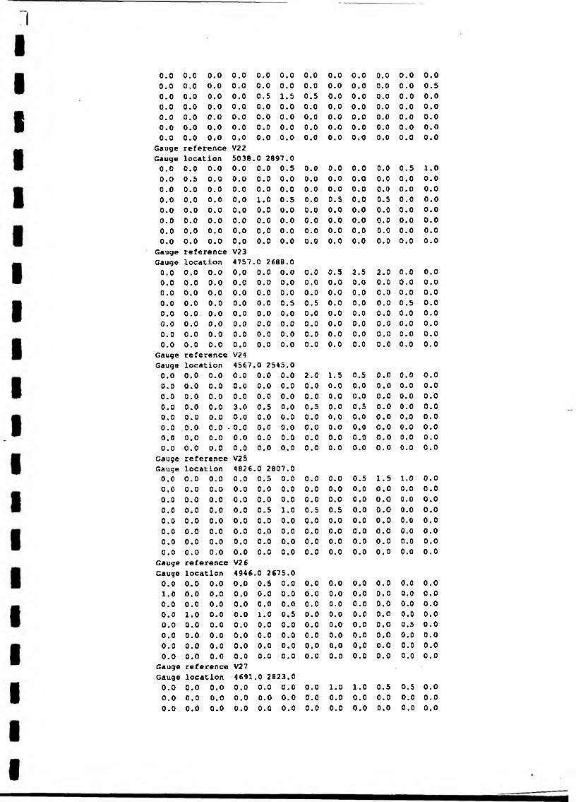
0.0 0.0 0.0 0.0 0.0 0.0 0.0 0.0 0.0 0.0 0.0 0.00.0 0.0 0.0 0.0 0.0 0.0 0.0 0.0 0.0 0.0 0.0 0.50.0 0.0 0.0 0.0 0.5 1.5 0.5 0.0 0.0 0.0 0.0 0.00.0 0.0 0.0 0.0 0.0 0.0 0.0 0.0 0.0 0.0 0.0 0.00.0 0.0 0.0 0.0 0.0 0.0 0.0 0.0 0.0 0.0 0.0 0.00.0 0.0 0.0 0.0 0.0 0.0 0.0 0.0 0.0 0.0 0.0 0.00.0 0.0 0.0 0.0 0.0 0.0 0.0 0.0 0.0 0.0 0.0 0.0Gauge reference V22Gauge location 5038.,0 2897.00.0 0.0 0.0 0.0 0.0 0.5 0.0 0.0 0.0 0.0 0.5 1.00.0 0.5 0.0 0.0 0.0 0.0 0.0 0.0 0.0 0.0 0.0 0.00.0 0.0 0.0 0.0 0.0 0.0 0.0 0.0 0.0 0.0 0.0 0.00.0 0.0 0.0 0.0 1.0 0.5 0.0 0.5 0.0 0.5 0.0 0.00.0 0.0 0.0 0.0 0.0 0.0 0.0 0.0 0.0 0.0 0.0 0.00.0 0.0 0.0 0.0 0.0 0.0 0.0 0.0 0.0 0.0 0.0 0.00.0 0.0 0.0 0.0 0.0 0.0 0.0 0.0 0.0 0.0 0.0 0.00.0 0.0 0.0 0.0 0.0 0.0 0.0 0.0 0.0 0.0 0.0 0.0Gauge reference V23Gauge location 4757 ..0 2688.00.0 0.0 0.0 0.0 0.0 0.0 0.0 0.5 2.5 2.0 0.0 0.00.0 0.0 0.0 0.0 0.0 0.0 0.0 0.0 0.0 0.0 0.0 0.00.0 0.0 0.0 0.0 0.0 0.0 0.0 0.0 0.0 0.0 0.0 0.00.0 0.0 0.0 0.0 0.0 o .s 0.5 0.0 0.0 0.0 0.5 0.00.0 0.0. 0.0 0.0 0.0 0.0 0.0 0.0 0.0 0.0 0.0 0.00.0 0.0 0.0 0.0 0.0 0.0 0.0 0.0 0.0 0.0 0.0 0.00.0 0.0 0.0 0.0 0.0 0.0 0.0 0.0 0.0 0.0 0.0 0.00.0 0.0 0.0 0.0 0.0 0.0 0.0 0.0 0.0 0.0 0.0 0.0
Gauge reference V24Gauge location 4567,,0 2545.00.0 0.0 0.0 0.0 0.0 0.0 2.0 1.5 0.5 0.0 0.0 0.00.0 0.0 0.0 0.0 0.0 0.0 0.0 0.0 0.0 0.0 0.0 0.00.0 0.0 0.0 0.0 0.0 0.0 0.0 0.0 0.0 0.0 0.0 0.00.0 0.0 0.0 3.0 0.5 0.0 0.5 0.0 0.5 0.0 0.0 0.00.0 0.0 0.0 0.0 0.0 0.0 0.0 0.0 0.0 0.0 0.0 0.00.0 0.0 0.0 - 0.0 0.0 0.0 0.0 0.0 0.0 0.0 0.0 0.00.0 0.0 0.0 0.0 0.0 0.0 0.0 0.0 0.0 0.0 0.0 0.00.0 0.0 0.0 0.0 0.0 0.0 0.0 0.0 0.0 0.0 0.0 0.0
Gauge reference V25Gauge location 4826..0 2807.0
0.0 0.0 0.0 0.0 0.5 0.0 0.0 0.0 0.5 1.5 1.0 0.00.0 0.0 0.0 0.0 0.0 0.0 0.0 0.0 0.0 0.0 0.0 0.00.0 0.0 0.0 0.0 0.0 0.0 0.0 0.0 0.0 0.0 0.0 0.00.0 0.0 0.0 0.0 0.5 1.0 0.5 0.5 0.0 0.0 0.0 0.00.0 0.0 0.0 0.0 0.0 0.0 0.0 0.0 0.0 0.0 0.0 0.00.0 0.0 0.0 0.0 0.0 0.0 0.0 0.0 0.0 0.0 0.0 0.00.0 0.0 0.0 0.0 0.0 0.0 0.0 0.0 0.0 0.0 0.0 0.00.0 0.0 0.0 0.0 0.0 0.0 0.0 0.0 0.0 0.0 0.0 0.0
Gauge reference V26Gauge location 4946.0 2675.00.0 0.0 0.0 0.0 0.5 0.0 0.0 0.0 0.0 0.0 0.0 0.01.0 0.0 0.0 0.0 0.0 0.0 0.0 0.0 0.0 0.0 0.0 0.00.0 0.0 0.0 0.0 0.0 0.0 0.0 0.0 0.0 0.0 0.0 0.00.0 1.0 0.0 0.0 1.0 0.5 0.0 0.0 0.0 0.0 0.0 0.00.0 0.0 0.0 0.0 0.0 0.0 0.0 0.0 0.0 0.0 0.5 0.00.0 0.0 0.0 0.0 0.0 0.0 0.0 0.0 0.0 0.0 0.0 0.00.0 0.0 0.0 0.0 0.0 0.0 0.0 0.0 0.0 0.0 0.0 0.00.0 0.0 0.0 0.0 0.0 0.0 0.0 0.0 0.0 0.0 0.0 0.0
Gauge reference V27Gauge location 4 691 .0 2823.00.0 0.0 0.0 0.0 0.0 0.0 0.0 1.0 1.0 0.5 0.5 0.00.0 0.0 0.0 0.0 0.0 0.0 0.0 0.0 0.0 0.0 0.0 0.00.0 0.0 0.0 0.0 0.0 0.0 0.0 0.0 0.0 0.0 0.0 0.0
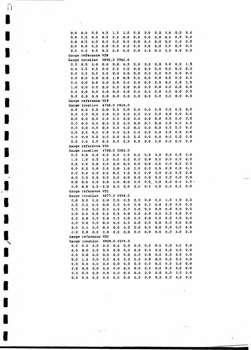
0.0 0.0 0.0 4.5 1.5 1.0 0.5 0.0 0.0 0.0 •0.0 0.00.0 0.0 0.0 0.0 0.0 0.0 0.0 0.0 0.0 0.0 0.0 0.00.0 o:o 0.0 0.0 0.0 0.0 0.0 0.0 0.0 0.0 0.0 0.00.0 0.0 0.0 0.0 0.0 0.0 0.0 0.0 0.0 0.0 0.0 0.00.0 0.0 0.0 0.0 0.0 0.0 0.0 0.0 0.0 0.0 0.0 0.0
Gauge reference V28Gauge location 5090..0 2962.00.0 0.0 0.0 0.0 0.0 0.5 0.0 0.0 0.0 0.0 0.0 1.50.5 0.5 0.0 0.0 0.0 0.0 0.0 0.0 0.0 0.0 0.0 0.00.0 0.0 0.0 0.0 0.0 0.0 0.0 0.0 0.0 0.0 0.0 0.00.0 0.0 0.0 0.0 1.0 0.5 0.0 0.0 0.0 0.0 0.0 0.00.0 0.0 0.0 0.0 0.0 0.0 0.0 0.0 0.5 0.5 0.5 1.51.0 0.0 0.0 0.0 0.0 0.0 0.0 0.0 0.0 0.0 0.0 0.00.0 0.0 0.0 0.0 0.0 0.0 0.0 0.0 0.0 0.0 0.0 0.00.0 0.0 0.0 0.0 0.0 0.0 0.0 0.0 0.0 0.0 0.0 0.0
Gauge reference V29Gauge location 4768,.0 2616.00.0 0.0 0.0 0.0 0.5 0.0 0.0 0.0 0.0 0.5 0.5 0.00.0 0.0 0.0 0.0 0.0 0.0 0.0 0.0 0.0 0.0 0.0 0,00.0 0.0 0.0 0.0 0.0 0.0 0.0 0.0 0.0 0.0 0.0 0.00.0 0.0 0.0 0.0 0.5 0.0 0.0 0.5 0.0 0,0 0.0 0.00.0 0.0 0.0 0.5 0.0 0.0 0.0 0.0 0.0 0.0 0.0 0.00.0 0.0 0.0 0.0 0.0 0.0 0.0 0.0 0.0 0.0 0.0 0.00.0 0.0 0.0 0.0 0.0 0.0 0.0 0.0 0.0 0.0 0.0 0.00.0 0.0 0.0 0.0 0.0 0.0 0.0 0.0 0.0 0.0 0.0 0.0Gauge reference V30Gauge location 4760 .0 3005.00.0 0.0 0.0 0.0 0.5 0.5 0.5 0.5 0.0 0.5 0.0 0.01.5 1.0 0.5 1.0 0.0 0.0 0.0 0.0 0.0 0.0 0.0 0.00.0 0.0 0.0 0.0 0.0 0.0 0.0 0.0 0.0 0.0 0.0 0.00.0 0.0 0.0 0.0 0.0 1.0 2.0 0.0 0.5 0.0 0.0 0.00.0 0.0 0.0 0.0 0.0 0.0 0.0 0.0 0.0 0.0 0.5 0.00.0 0.0 0.0 0.0 0.0 0.0 0.0 0.0 0.0 0.0 0.0 0.00.0 0.0 0.0 0.0 0.0 0.0 0.0 o.'o_ 0,.0_ 0.0 0.0 0.00.0. 0.0 0.0 --0.0' 0.0 0.0 0^0 0.0 0.0 0.0 0.0 0.0
Gauge reference V31Gauge location 4877 .0 2994.00.0 0.0 0.0 0.0 0.5 0,5 0.0 0.0 0.0 1.5 1.0 0.50.5 0.5 0.0 0.0 0.0 0.0 0.0 0.0 0.0 0.0 0.0 0.00.0 0.0 0.0 0.0 0.0 0.0 0.0 0.0 0.0 0.0 0.0 0.00.0 0.0 0.0 0.5 0.5 0.0 0.0 0.0 0.0 0.0 0.0 0.00.0 0.0 0.0 0.0 0.0 0.0 0.0 0.0 0.0 0.0 0.0 0.00.0 0.0 0.0 0.0 0.0 0.0 0.0 0.0 0.0 0.0 0.0 0.00.0 0.0 0.0 0.0 0.0 0.0 0.0 0.0 0.0 0.0 0.0 0.00.0 0.0 0.0 0.0 0.0 0.0 0.0 0.0 0.0 0.0 0.0 0.0Gauge reference V32Gauge location 4908.0 2674.00.0 0.0 0.0 0.0 0.0 0.0 0.0 0.0 0.5 0.0 0.0 0.00.0 0.0 0.0 0.0 0.0 0.0 0.0 0.0 0.0 0.0 0.0 0.00.0 0.0 0.0 0.0 0.0 0.0 0.0 0.0 0.0 0.0 0.0 0.00.0 1.5 0.0 0.5 0.0 2.0 0.0 0.0 0.0 0.0 0.0 0.00.0 0.0 0.0 0.0 0.0 0.0 0.0 0.0 0.0 0.0 0.0 0.00.0 0.0 0.0 0.0 0.0 0.0 0.0 0.0 0.0 0.0 0.0 0.00.0 0.0 0.0 0.0 0.0 0.0 0.0 0.0 0.0 0.0 0.0 0.00.0 0.0 0.0 0.0 0.0 0.0 0.0 0.0 0.0 0.0 0.0 0.0


Appendix 4: Example Q trhmp.m Tnpntfile
This catchment file contains data for one catchment and contains node co-ordinates for all nodes falling within the catchment in NGR coordinates (5 km grid resolution).
Catchment datafile for use with QUANTAREPile contains ngr's of points falling within pre-defined catchments Example catchment datafile 1Test catchment: 100 sq km (10 km * 10 km)94850.0 2650.04900.0 2850.04950.0 2850.04950.0 2900.04950.0 2950.04900.0 2950.04850.0 2950.04850.0 2900.04900.0 2900.0
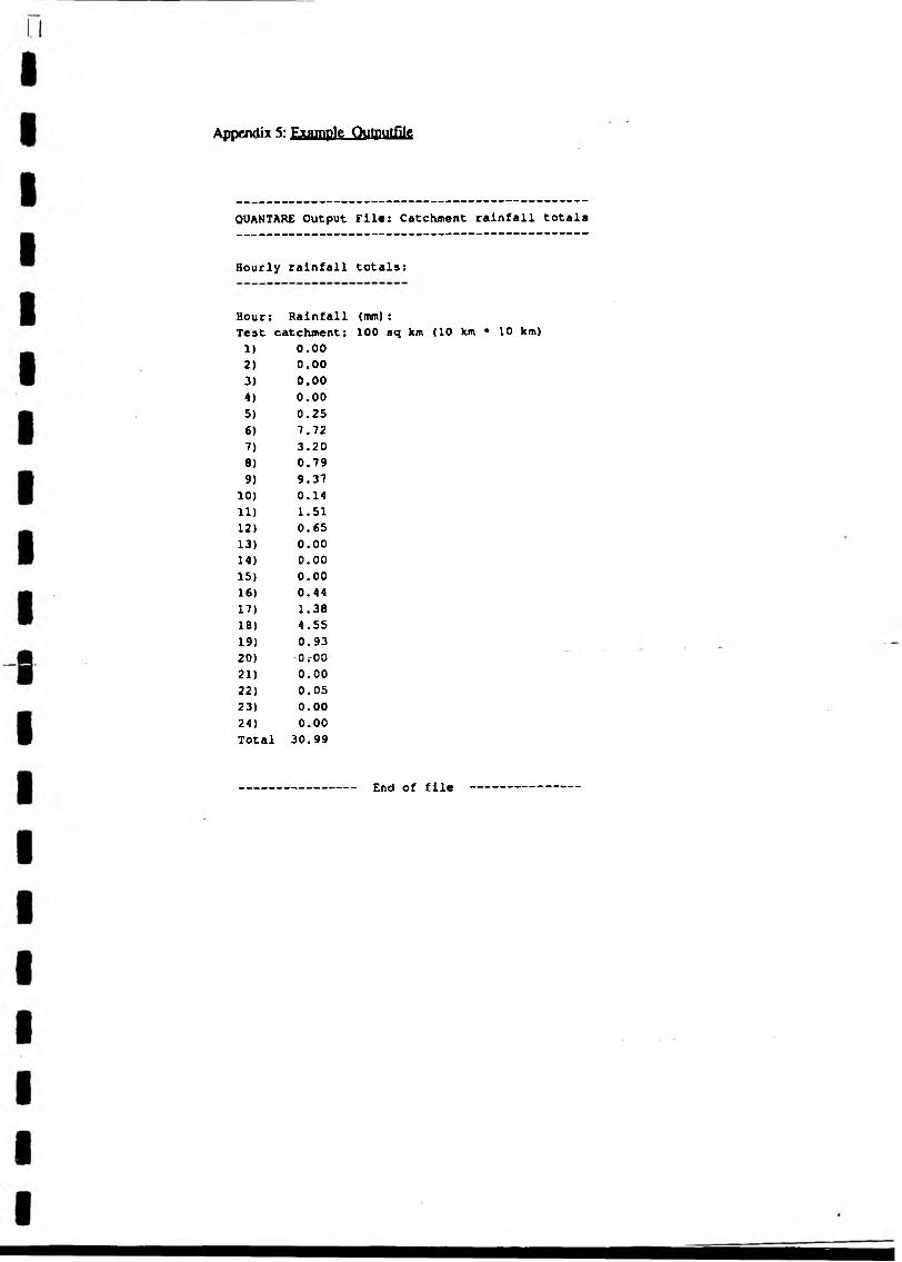
Appendix 5: Example OutPutffle
QUANTARE Output File: Catchment rainfall totals
Hourly rainfall totals:
Hour: Rainfall (mm):Test catchment: 100 sq km (10 km * 10 km)1) 0.002 ) 0 .0 03) 0.004) 0.005) 0.256) 7.727) 3.208) 0.799) 9.3710) 0.1411) 1.5112) 0.6513) 0.0014) 0.0015) 0.0016) 0.4417) 1.3818) 4.5519) 0.9320) -OrOO21) 0.0022) 0.0523) 0.0024) 0.00 Total 30.99
End of file
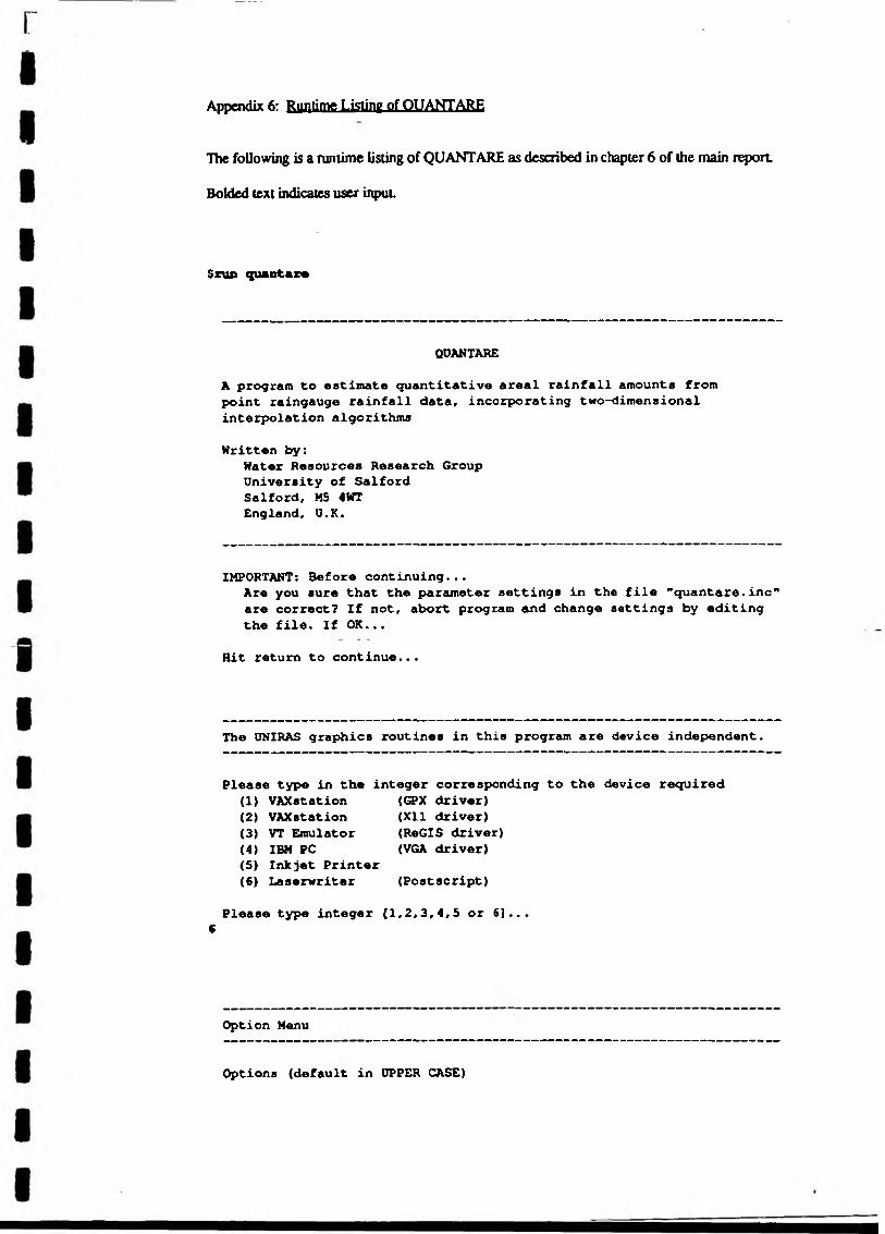
The following is a runtime listing of QUANTARE as described in chapter 6 of the main report
Bolded text indicates user inpuL
$rua qpiintiri
Appendix 6: Runtime Listing of QUANTARE
QUANTARE
A program to estimate quantitative areal rainfall amounts from point raingauge rainfall data, incorporating two-dimensional interpolation algorithms
Written by:Water Resources Research Group University of Salford Salford, M5 4WT England, U.K.
IMPORTANT: Before continuing...Are you sure that the parameter settings in the file "quantare.inc" are correct? If not, abort program and change settings by editing the file. If OK...
Hit return to continue...
The UNIRAS graphics routines in this program are device independent.
Please type in the integer corresponding to the device required(1) VAXstation (GPX driver)(2) VAXstation (XI1 driver)(3) VT Emulator (ReGIS driver)(4) IBM PC (VGA driver)(5) Inkjet Printer(6) LaserWriter (Postscript)
Please type integer (1,2,3,4,5 or 6]...6
Option Menu
Options (default in UPPER CASE)
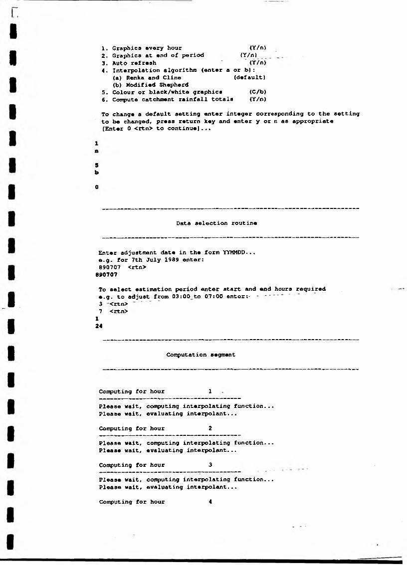
er w
1. Graphics every hour (Y/n)2. Graphics at end of period (Y/n)3. Auto refresh (Y/n)4. Interpolation algorithm (enter a or b):
(a) Renka and Cline (default)(b) Modified Shepherd
5. Colour or black/white graphics (C/b)6. Compute catchment rainfall totals (Y/n)
To change a default setting enter integer corresponding to the setting to be changed, press return key and enter y or n as appropriate [Enter 0 <rtn> to continue]...
Data selection routine
Enter adjustment date in the form YYMMDD... e.g. for 7th July 1989 enter:890707 <rtn>890707
To select estimation period enter start and end hours required e.g. to adjust from 03:00_to 07:00 entor:- -3 -<rtn>7 <rtn>124
Computation segment
Confuting for hour 1
Please wait, computing interpolating function... Please wait, evaluating interpolant...
Computing for hour 2
Please wait, computing interpolating function... Please wait, evaluating interpolant...
Computing for hour 3
Please wait, computing interpolating function... Please wait, evaluating interpolant...
Computing for hour 4

Please wait,-computing interpolating function. Please wait, evaluating interpolant...
Confuting for hour 5
Please wait, computing interpolating function. Please wait, evaluating interpolant...
Computing for hour 6
Please wait, computing interpolating function. Please wait, evaluating interpolant...
Computing for hour 7
Please wait, computing interpolating function. Please wait, evaluating interpolant...
Computing for hour 8
Please wait, computing interpolating function. Please wait, evaluating interpolant...
Computing for hour
Please wait, computing interpolating function. Please wait, evaluating interpolant...
Confuting for hour 10
Please wait, computing interpolating function. Please wait, evaluating interpolant...
Computing for hour 11
Please wait, computing interpolating function. Please wait, evaluating interpolant...
Computing for hour 12
Please wait, computing interpolating function. Please wait, evaluating interpolant...
Computing for hour 13
Please wait, computing interpolating function. Please wait, evaluating interpolant...
Computing for hour 14
Please wait, computing interpolating function. Please wait, evaluating interpolant...
Computing for hour IS
Please wait, computing interpolating function. Please wait, evaluating interpolant...
Computing for hour 16
Please wait, computing interpolating function. Please wait, evaluating interpolant...
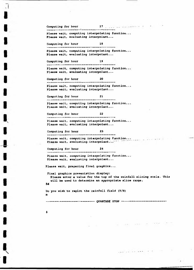
Computing for hour 17
Please wait, computing interpolating function... Please wait, evaluating interpolant.,.
Computing for hour 16
Please wait, computing interpolating function... Please wait, evaluating interpolant...
Computing for hour 19
Please wait, computing interpolating function... Please wait, evaluating interpolant...
Computing for hour 20
Please wait, computing interpolating function... Please wait, evaluating interpolant...
Computing for hour 21
Please wait, computing interpolating function... Please wait, evaluating interpolant...
Computing for hour 22
Please wait, computing interpolating function... Please wait, evaluating interpolant...
Computing for hour 23
Please wait, computing interpolating function... Please wait, evaluating-interpolant'.'..
Computing for hour 24
Please wait, computing interpolating function...Please wait, evaluating interpolant...
Please wait, preparing final graphics...
Final graphics presentation display:Please enter a value for the top of the rainfall slicing scale. This will be used to determine an appropriate slice range.
56
Do you wish to replot the rainfall field (Y/N) n
------------------------- QUANTARE STOP -----------------------
$

I
4400 5400
4400 5400Eat ting (NGR)
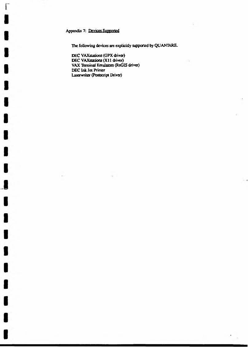
Appendix 7: Devices Supported
The following devices are explicitly supported by QUANTARE.
DEC VAXstations (GPX driver)DEC VAXstations (XI1 driver)VAX ’Terminal Emulators (ReGIS driver)DEC Ink Jet Printer LaserWriter (Postscript Driver)
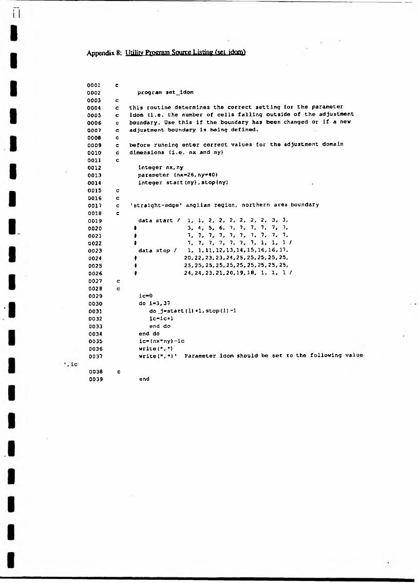
Appendix 8: Utility Program Source Listing (set idom)
0001 c0002 program set_idom0003 c0004 c this routine determines the correct setting for the parameter0005 c idom (i.e. the number of cells falling outside of the adjustment0006 c boundary. Use this if the boundary has been changed or if a new0007 c adjustment, boundary is being defined.0008 c0009 c before running enter correct values for the adjustment domain0010 c dimensions (i.e. nx and ny)0011 c0012 integer nx,ny0013 parameter (nx«26,ny-40)0014 integer start(ny),stop(ny)0015 c0016 c0017 c 'straight-edge' anglian region, northern area boundary0018 c0019 data start / 1, 1, 2, 2, 2, 2, 2, 2, 3, 3,0020 # 3, 4, 5, 6, 7, 7, 7, 7, 7, 7,0021 * 7, 7, 7, 7, 7, 7, 7. 7, 7, 7,0022 # 7, 7, 7, 7, 7, 7, 7, 1, 1, 1 /0023 data stop / 1, 1,11,12,13,14,15,16,16,17,0024 ♦ 20. 22, 23, 23,24,25, 25,25,25, 25,0025 # 25, 25, 25, 25, 25, 25, 25,25,25,25,0026 I 24,24,23,21,20,19, 18, 1, 1. 1 /0027 c0028 c0029 ic-00030 do i«*3,370031 do _j*start(i)+1,stop(i)-10032 ic-ic+10033 end do0034 end do0035 ic-(nx*ny)-ic0036 write(*,*)0037 write (*,*)' Parameter idom should be set to the following val
0038 c0039 end


![PHOSPHATE IN THE CUT-OFF CHANN]ea-lit.freshwaterlife.org/fedora/repository/ealit:4167/...SIMCAT can calibrate automatically. In this study, auto-calibration was used to](https://img.pdfslide.net/doc/110x75/606dfefe1859b37b04179e60/phosphate-in-the-cut-off-channea-lit-4167-simcat-can-calibrate-automatically.jpg)