UT Dallas 4-05-05

Wavelet-Based Preprocessing Methods for Mass Spectrometry Data

Jeffrey S. MorrisDepartment of Biostatistics and Applied

MathematicsUT M.D. Anderson Cancer Center

UT Dallas 4-05-05

Overview

Background and MotivationPreprocessing Steps

Denoising using WaveletsBaseline Correction/NormalizationPeak Detection/QuantificationWorking with Average Spectrum

Virtual Mass SpectrometerSimulation StudyConclusions

UT Dallas 4-05-05

Example: MALDI-MS

Central dogma: DNA mRNA proteinMicroarrays: measure expression levels of 10,000s of genes in sample (amount of mRNA) Proteomics: look at proteins in sample.

Gaining increased attention in research• Proteins more biologically relevant than mRNA • Can use readily available fluids (e.G. Blood, urine)

MALDI-TOF: mass spectrometry instrument that can see 100s or 1000s of proteins in sample

UT Dallas 4-05-05

MALDI-TOF schematic

Vestal and Juhasz. J. Am. Soc. Mass Spectrom. 1998, 9, 892.

UT Dallas 4-05-05

Raw Spectrum

UT Dallas 4-05-05

Statistical Issues for Mass Spectrometry Experiments

Experimental DesignBlocking/RANDOMIZATION – reduce possibility of systematic bias polluting the data.

PreprocessingRemove systematic artifacts/noise from dataExtract meaningful features (protein signal) : nxp matrix

Data Analysis/DiscoveryAnalyze n x p matrix • Find which features are associated with exp. cond.• Build/validate classifier based on sets of features• Cluster samples/features

Lots of existing methods available for this

UT Dallas 4-05-05

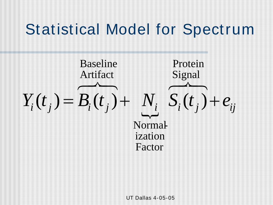
Statistical Model for Spectrum

ijjiijiji etSNtBtY ++= )()()(

UT Dallas 4-05-05

Statistical Model for Spectrum

ijjiijiji etSNtBtY ++= )()()(ArtifactBaseline

876

UT Dallas 4-05-05

Statistical Model for Spectrum

ijjiijiji etSNtBtY ++=876876 Signal

ProteinArtifactBaseline

)()()(

UT Dallas 4-05-05

Statistical Model for Spectrum

{ ijjiijiji etSNtBtY ++=876876 Signal

Protein

Factor ization

-Normal

ArtifactBaseline

)()()(

UT Dallas 4-05-05

Statistical Model for Spectrum

{ {

(detector) noise

additive

SignalProtein

Factor ization

-Normal

ArtifactBaseline

)()()( ijjiijiji etSNtBtY ++=876876

)}(,0{~ 2jij tNe σ

UT Dallas 4-05-05

Preprocessing

Goal: Isolate protein signal Si(tj)Filter out baseline and noise, normalizeExtract individual features from signal

Problem:Baseline removal, denoising, normalization, and feature extraction are interrelated processes.Where do we start?

UT Dallas 4-05-05

Denoising using Wavelets

First step: Isolate noise using waveletsWavelets: basis functions that can parsimoniously represent spiky functionsStandard denoising tool in signal processing

Idea: Transform from time to wavelet domain, threshold small coefficients, transform back.

Result: Denoised function and noise estimateWhy does it work? Signal concentrated on few wavelet coefficients, white noise equally distributed.Thresholding removes noise without affecting signal.

Does much better than denoising tools based on kernels or splines, which tend to attenuate peaks in the signal when removing the noise.

UT Dallas 4-05-05

Raw Spectrum

UT Dallas 4-05-05

Denoised Spectrum

UT Dallas 4-05-05

Noise

UT Dallas 4-05-05

Baseline Correction & Normalization

Baseline: smooth artifact, largely attributable to detector overload.

Estimated by monotone local minimumMore stably estimated after denoising

Normalization: adjust for possibly different amounts of material desorbing from plates

Divide by total area under the denoised and baseline corrected spectrum.

UT Dallas 4-05-05

Baseline Estimate

UT Dallas 4-05-05

Denoised, Baseline Corrected Spectrum

UT Dallas 4-05-05

Denoised, Baseline Corrected, and Normalized Spectrum

UT Dallas 4-05-05

Protein SignalIdeal Form of Protein Signal:Convolution of peaks

Proteins, peptides, and their alterationsAlterations: isotopes; matrix/sodium adducts; neutral losses of water, ammonia, or carbon

Limitations of instrument used means we may not be able to resolve all peaks.Advantages of peak detection:

Reduces multiplicity problemFocuses on units that are theoretically the scientifically interesting features of the data.

UT Dallas 4-05-05

Peak DetectionEasy to do after other preprocessingAny local maximum after denoising, baseline correction, and normalization is assumed to correspond to a “peak”.May want to require S/N>δ to reduce number of spurious peaks.

We can estimate the noise process σ(t) by applying a local median to the filtered noise from the wavelet transform.

Signal-to-noise estimate is ratio of preprocessed spectrum and noise.

UT Dallas 4-05-05

Peak Detection

3326 locations, 81 peaks

UT Dallas 4-05-05

Peak Detection (zoomed)

UT Dallas 4-05-05

Raw Spectrum with peaks

UT Dallas 4-05-05

Peak QuantificationTwo options:

1. Area under the peak: Find the left and right endpoints of the peak, compute the AUC in this interval.

2. Maximum intensity: Take intensity at the local maximum (may want to take log or cube root)

Theoretically, AUP quantifies amount of given substance desorbed from the chip.

But it is very difficult to identify the endpoints of peaks

UT Dallas 4-05-05

Peak QuantificationThe maximum intensity is a practical alternative

No need for endpoints, should be correlated with AUPPhysics of mass spectrometry shows that, for a given ion with m/z value x, there is a linear relationship between the number of ions of that type desorbed from plate and the expected maximum peak intensity at x.

Problem with both methods: Overlapping peaks that are not deconvolvable

Local maximum at t contains weighted average of information from multiple ions whose corresponding peaks have mass at location t.Major problem – short of formal deconvolution, have not seen simple solution to this problem.

UT Dallas 4-05-05

Peak Matching Problem

If peak detection performed on individual spectra, peaks must be matched across samples to get n x p matrix.

Difficult and arbitrary processWhat to do about “missing peaks?”

Our Solution: Identify peaks on mean spectrum (at locations x1, …, xp), then quantify peaks on individual spectra by intensities at these locations.

UT Dallas 4-05-05

Advantages/Disadvantages

AdvantagesAvoids peak-matching problemGenerally more sensitive and specific• Noise level reduced by sqrt(n)• Borrows strength across spectra in

determining whether there is a peak or not (signals reinforced over spectra)

Robust to minor calibration problemsDisadvantage

Tends to be less sensitive when prevalence of peak < 1/sqrt(n).

UT Dallas 4-05-05

Noise reduced in mean spectrum

UT Dallas 4-05-05

Noise reduced in mean spectrum

UT Dallas 4-05-05

Peak detection with mean spectrum

UT Dallas 4-05-05

Sample Spectrum

UT Dallas 4-05-05

Simulated spectraDifficult to evaluate processing methods on real data since we don’t know “truth”Have developed a simulation engine to produce realistic spectra

Based on the physics of a linear MALDI-TOF with ion focus delayFlexible incorporation of different noise models and different baseline modelsIncludes isotope distributionsCan include matrix adducts, other modifications

UT Dallas 4-05-05

MALDI-TOF schematic

Vestal and Juhasz. J. Am. Soc. Mass Spectrom. 1998, 9, 892.

UT Dallas 4-05-05

Modeling the physics of MALDI-TOF

ParametersD1 = distance from

sample plate to first grid (8 mm)

V1 = voltage for focusing (2000 V)

D2 = distance between grids (17 mm)

V2 = voltage for acceleration(20000 V)

L = length of tube (1 m)v0 = initial velocity ~

N(µ,σ)v1 = velocity after

focusingδ= delay time

Equations

)(201

1

120

21 vD

mDqVvv δ−+=

⎟⎠⎞

⎜⎝⎛ += 2

1222 2/ v

mqVLtDRIFT

⎟⎟⎠

⎞⎜⎜⎝

⎛−= 1

2

2 vt

LqVmDt

DRIFTACCEL

( )011

1 vvqVmDtFOCUS −=

UT Dallas 4-05-05

Simulation of one protein, with isotope distribution

UT Dallas 4-05-05

Same protein simulated on a low resolution instrument

UT Dallas 4-05-05

Simulation of one protein with matrix adducts

UT Dallas 4-05-05

Simulated calibration spectrum with equal amounts of six proteins

UT Dallas 4-05-05

Simulated spectrum with a complex mixture of proteins

UT Dallas 4-05-05

Closeup of simulated complex spectrum

UT Dallas 4-05-05

Real and Virtual Spectra

UT Dallas 4-05-05

Using Virtual Mass Spectrometer

Input: virtual sampleproteins and peptides desorbed from samplelist of molecular masses w/ # of molecules

Output: virtual spectrumSimulation Studies: virtual population

Defines distribution of proteins in proteome from which you are samplingAssume p proteins; for each specify 4 quantities

• major peak location (m/z of dominant ion)• prevalence (proportion of samples with protein)• abundance (mean # ions desorbed from samples w/ protein)• variance (var # of desorbed ions across samples w/ protein)

UT Dallas 4-05-05

Simulation Study

1. Generated 100 random virtual populations based on MDACC MALDI study on pancreatic cancer.

2. For each virtual population, generated 100 virtual samples, obtained 100 virtual spectra.

3. Applied preprocessing and peak detection method based on individual and average spectra

4. Summarized performance based on sensitivity (proportion of proteins detected) and FDR (proportion of peaks corresponding to real proteins).

Tricky to do – see paper for details.

UT Dallas 4-05-05

Simulation ResultsOverall Results

sensitivity FDR pv*

SUDWT(indiv. spectra)

0.75 0.09 0.03

MUDWT(mean spectrum)

0.83 0.06 0.97

*pv=the proportion of simulations with higher sensitivity

UT Dallas 4-05-05

Simulation ResultsBy Prevalence

π: <.05(14%)

.05-.20(16%)

.20-.80(40%)

>.80(30%)

sensitivity (SUDWT)

0.43 0.74 0.81 0.82

sensitivity (MUDWT)

0.38 0.74 0.93 0.97

pv(MUDWT)

0.25 0.49 1.00 1.00

UT Dallas 4-05-05

Simulation ResultsBy Abundance (mean log intensity)

log(µ): <9.0(31%)

9.0-9.5(27%)

9.5-10(23%)

>10(19%)

sensitivity (SUDWT)

0.68 0.75 0.78 0.82

sensitivity (MUDWT)

0.78 0.84 0.85 0.88

pv(MUDWT)

0.97 0.89 0.84 0.78

UT Dallas 4-05-05

ConclusionWavelet-Based Preprocessing:Coombes KR, Tsavachidis S, Morris JS, Baggerly KA, and Kuerer HM: Improved Peak Detection and Quantification of Mass Spectrometry Data Acquired from Surface-Enhanced Laser Desorption and Ionization by Denoising Spectra with theUndecimated Discrete Wavelet Transform. Proteomics, to appear 2005.Using Average Spectrum for Preprocessing:Morris JS, Coombes KR, Kooman J, Baggerly KA, and Kobayashi R: Feature Extraction and Quantification for Mass Spectrometry Data in Biomedical Applications Using the Mean Spectrum.Bioinformatics, 22 Feb 2005: Epub ahead of print.Virtual Mass Spectrometer:Coombes KR, Koomen, JM, Baggerly KA, Morris JS, and Kobayashi R: Understanding the characteristics of mass spectrometry data through the use of simulation. Cancer Informatics, to appear 2005. Website: http://bioinformatics.mdanderson.org/

Contains code for preprocessing (Cromwell) and simulation engine, plus some publically available mass spectrometry data sets.

UT Dallas 4-05-05

Open problems: Preprocessing

Better calibration?Internal validation

Better baseline correction?Alternative methods for normalization?Quality control/quality assurance?Best approach for quantification?

UT Dallas 4-05-05

Open problems: Virtual Mass Spectrometry Instrument

Include more alterationsAdducts and neutral molecule lossesMultiply-charged ions

Develop more realistic model for baseline artifactGeneralize to other instruments?

UT Dallas 4-05-05

AcknowledgementsBioinformatics

Kevin CoombesKeith BaggerlyJianhua HuJing WangLianchun XiaoSpyros TsavachidisThomas Liu

Proteomics (MDACC)Ryuji KobayashiDavid Hawke John Koomen

CiphergenCharlotte Clarke

Biologists (MDACC)Jim AbbruzzeseI.J. FidlerStan HamiltonNancy ShihKen AldapeHenry KuererHerb FritscheGordon MillsLajos PusztaiJack RothLin Ji