Embed Size (px)
Citation preview
Geophys. J. Int. (2005) 163, 875–899 doi: 10.1111/j.1365-246X.2005.02754.x
GJI
Geo
des
y,pote
ntialfiel
dand
applie
dgeo
phys
ics
Wavelet frames: an alternative to spherical harmonic representationof potential fields
A. Chambodut,1∗ I. Panet,2,3 M. Mandea,1† M. Diament,2 M. Holschneider4
and O. Jamet31Laboratoire de Geomagnetisme et Paleomagnetisme, UMR 7577, Institut de Physique du Globe de Paris, France. E-mail: [email protected] de Gravimetrie et Geodynamique, Departement de Geophysique Spatiale et Planetaire, UMR 7096, Institut de Physique du Globe de Paris,
France3Laboratoire de Recherche en Geodesie, Institut Geographique National, France4Department of Applied and Industrial Mathematics, University of Potsdam, Germany
Accepted 2005 July 19. Received 2005 June 1; in original form 2004 September 14
S U M M A R Y
Potential fields are classically represented on the sphere using spherical harmonics. However,
this decomposition leads to numerical difficulties when data to be modelled are irregularly dis-
tributed or cover a regional zone. To overcome this drawback, we develop a new representation
of the magnetic and the gravity fields based on wavelet frames.
In this paper, we first describe how to build wavelet frames on the sphere. The chosen frames
are based on the Poisson multipole wavelets, which are of special interest for geophysical
modelling, since their scaling parameter is linked to the multipole depth (Holschneider et al.).
The implementation of wavelet frames results from a discretization of the continuous wavelet
transform in space and scale. We also build different frames using two kinds of spherical meshes
and various scale sequences. We then validate the mathematical method through simple fits of
scalar functions on the sphere, named ‘scalar models’. Moreover, we propose magnetic and
gravity models, referred to as ‘vectorial models’, taking into account geophysical constraints.
We then discuss the representation of the Earth’s magnetic and gravity fields from data regularly
or irregularly distributed. Comparisons of the obtained wavelet models with the initial spherical
harmonic models point out the advantages of wavelet modelling when the used magnetic or
gravity data are sparsely distributed or cover just a very local zone.
Key words: magnetic and gravity field, spherical harmonics, wavelets.
1 I N T RO D U C T I O N
Magnetic and gravity observations are of great importance for the
understanding of geodynamic activity of our planet. Measurements
of the Earth’s magnetic and gravity fields undertaken by satellites
(without forgetting those on land, sea and air) are of particular in-
terest, as they provide a global and uniform survey of these fields
and of their temporal evolution.
Models of the magnetic field have been derived by means of
several Earth’s satellite missions, which have been carrying mag-
netic sensors. Satellite-borne magnetometers provide information
on strength and direction of the internal and external Earth’s mag-
netic field and its time variations. The Earth is surrounded by a large
and complicated field caused to a large extent by a dynamo operating
∗Now at: Department of Applied and Industrial Mathematics, University of
Potsdam, Germany.
†Now at: GeoForschungsZentrum of Potsdam, Section 2.3: Geomagnetism,
Germany.
in the fluid core. Currents flowing in the ionosphere, magnetosphere
and oceans and magnetized rocks also influenced the geomagnetic
field.
Three magnetic missions (Ørsted—launched in 1999, CHAMP
and SAC-C—launched in 2000) have collected measurements pro-
viding new insights into the composition and the processes in the
interior, and surrounding of the planet. These observations are also
used in a range of applications, including navigation systems, re-
source exploration drilling, spacecraft attitude control systems and
assessments of the impact of space weather. The coming decade
will see further missions planned for more in-depth, dedicated stud-
ies of magnetic field including DEMETER, 2004; ESPERIA, 2006;
Swarm, 2008; etc.
Gravity field observations from space can advance our knowl-
edge of the geoid and its time variations. The geoid is the surface
of equal gravitational potential at mean sea level, and reflects the
irregularities in the Earth’s gravity field at its surface due to the
inhomogeneous mass and density distribution in the Earth’s inte-
rior. Such measurements are vital for quantitative determination, in
C© 2005 The Authors 875Journal compilation C© 2005 RAS
876 A. Chambodut et al.
combination with satellite altimetry, of permanent ocean currents,
for improvement of global height references, for the study of the
Earth’s internal structure, for estimates of the thickness of the polar
ice sheets and its variations and for estimates of the mass/volume
redistribution of freshwater in order to further understand the hy-
drological cycle.
Gravity field measurements often utilize combinations of differ-
ent instrument types in order to derive the necessary information:
single or multiple accelerometer, precise satellite orbit determina-
tion systems and satellite-to-satellite tracking systems. CHAMP
(resp. GRACE) gravity data have been providing new information
on the Earth’s gravity field since 2000 (resp. 2002). The future grav-
ity mission GOCE will provide data sets that are capable of deriving
the geoid with 1 cm accuracy and gravity anomalies up to 1 mGal
at 100 km resolution.
With the advent of space exploration and all of the subsequent
technological advancements it is possible to systematically study the
Earth as a whole entity. However, it is realized that to comprehend
the myriad of interactions between Earth systems, we must utilize a
multidisciplinary approach within which the mapping of the Earth’s
magnetic and gravity fields, to a high degree of accuracy and reso-
lution, plays a crucial role. High-resolution models of the magnetic
and gravity fields of the Earth help us to understand the structure
and the driving forces behind plate tectonics, lithospheric motions,
mantle convection and core fluid flows.
Until recently, magnetic and gravity models have been realized
by applying the same technique: the spherical harmonic analysis
(SHA). This method is well suited for global representations, but
is very demanding for high-resolution models. This is the main
reason why during the last years some other new methods have
been investigated. Among them, a promising approach emerges:
the wavelets technique. In the present paper the spherical wavelet
models are introduced as an alternative to spherical harmonic mod-
els of the Earth’s magnetic and gravity fields like IGRF, OIFM,
CM4 and, respectively, EIGEN-1S, EIGEN-2, EIGEN-GRACE01S,
GGM01S, UCPH2002 0.5, EGM96. Thereby the localizing prop-
erties of spherical wavelets and their approximating capacity are
shown. A detailed description of the inverse problems is given. We
validate the mathematical method through the simple fits of scalar
functions on the sphere: this approach will be referred to as the
‘scalar case’ in the following, and the derived representations as
‘scalar models’. Finally, we propose magnetic and gravity models:
this approach will be referred to as the ‘vectorial case’, and the
derived models as ‘vectorial models’.
2 S TAT E O F T H E P RO B L E M : G L O B A L
A N D R E G I O N A L M O D E L L I N G
2.1 Magnetic field
Current geomagnetic field models include contributions from the
core, crust, ionosphere and magnetosphere and are derived by a
joint analysis of ground-based and satellite magnetic observations.
In doing so, a separation of the magnetic field contributions at par-
ticular epoch is necessary, and their inadequate separation is one of
the limiting factors for a more accurate determination of the core
field, of its secular variation, and of the lithospheric field.
The standard method for modelling the three dimensional mag-
netic field is called SHA. In the following this method is summa-
rized; for the technical details, see books by Jacobs (1987) and Merill
et al. (1996). The internal part of the magnetic field is the negative
spatial gradient of a scalar potential V M (r ,θ ,φ ,t), which satisfies
Laplace’s equation. Each internal field model comprises a set of
spherical harmonics, each of which being a solution to Laplace’s
equation:
VM (r, θ, φ, t) = RE
N∑
ℓ=1
ℓ∑
m=0
(
RE
r
)ℓ+1
(
gmℓ (t) cos mφ + hm
ℓ (t) sin mφ)Pmℓ (cos θ
)
, (1)
where RE = 6371.2 km is the mean radius of the Earth, r ≥ RE
denotes the radial distance from the centre of the Earth, θ de-
notes the geocentric colatitude, φ denotes the east longitude, t is
the time, Pmℓ (cos θ ) are the Schmidt semi-normalized associated
Legendre functions of degree ℓ and order m and gmℓ (t) and hm
ℓ (t)
are the corresponding Gauss coefficients. The maximum spherical
harmonic degree of the expansion is N , which leads to N (N + 2) real
coefficients.
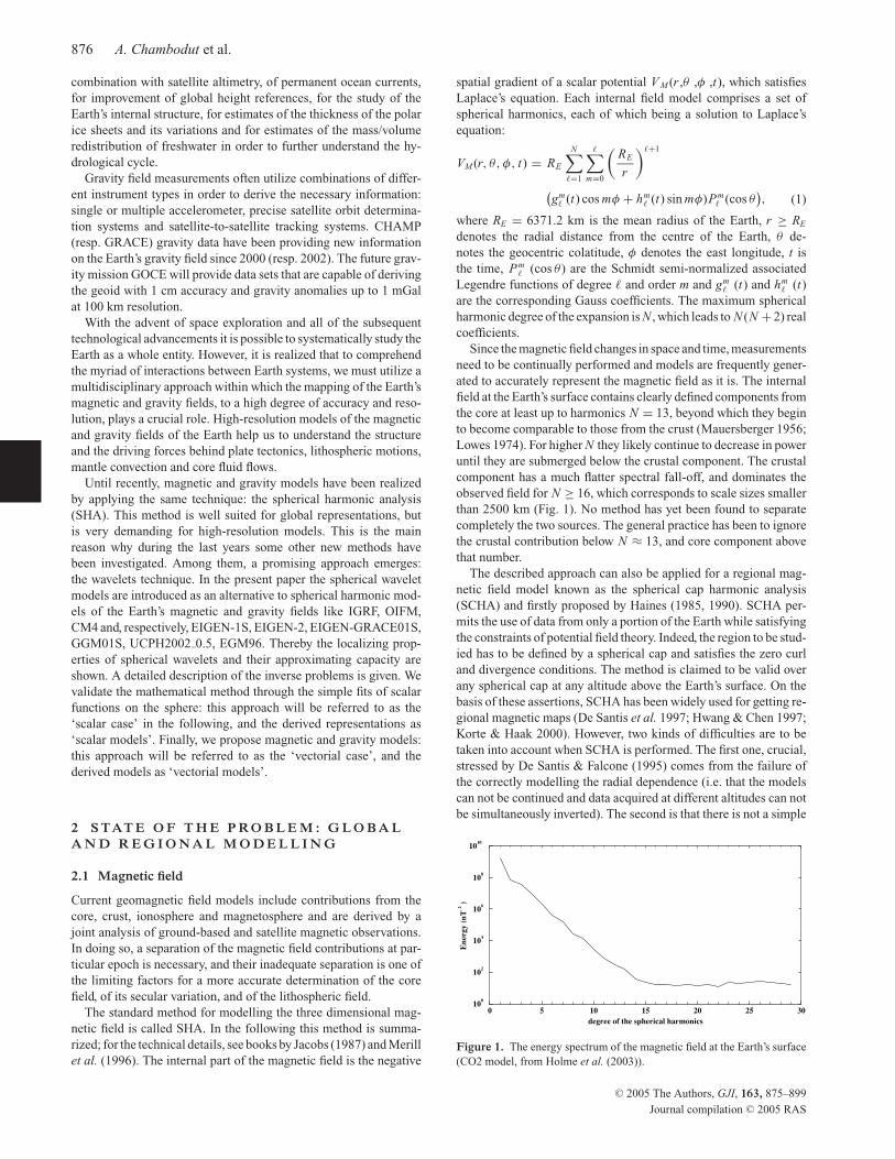
Since the magnetic field changes in space and time, measurements
need to be continually performed and models are frequently gener-
ated to accurately represent the magnetic field as it is. The internal
field at the Earth’s surface contains clearly defined components from
the core at least up to harmonics N = 13, beyond which they begin
to become comparable to those from the crust (Mauersberger 1956;
Lowes 1974). For higher N they likely continue to decrease in power
until they are submerged below the crustal component. The crustal
component has a much flatter spectral fall-off, and dominates the
observed field for N ≥ 16, which corresponds to scale sizes smaller
than 2500 km (Fig. 1). No method has yet been found to separate
completely the two sources. The general practice has been to ignore
the crustal contribution below N ≈ 13, and core component above
that number.
The described approach can also be applied for a regional mag-
netic field model known as the spherical cap harmonic analysis
(SCHA) and firstly proposed by Haines (1985, 1990). SCHA per-
mits the use of data from only a portion of the Earth while satisfying
the constraints of potential field theory. Indeed, the region to be stud-
ied has to be defined by a spherical cap and satisfies the zero curl
and divergence conditions. The method is claimed to be valid over
any spherical cap at any altitude above the Earth’s surface. On the
basis of these assertions, SCHA has been widely used for getting re-
gional magnetic maps (De Santis et al. 1997; Hwang & Chen 1997;
Korte & Haak 2000). However, two kinds of difficulties are to be
taken into account when SCHA is performed. The first one, crucial,
stressed by De Santis & Falcone (1995) comes from the failure of
the correctly modelling the radial dependence (i.e. that the models
can not be continued and data acquired at different altitudes can not
be simultaneously inverted). The second is that there is not a simple
0 5 10 15 20 25 30
degree of the spherical harmonics
100
102
104
106
108
1010
En
ergy (
nT
2 )
Figure 1. The energy spectrum of the magnetic field at the Earth’s surface
(CO2 model, from Holme et al. (2003)).
C© 2005 The Authors, GJI, 163, 875–899
Journal compilation C© 2005 RAS

Wavelet frames: an alternative to spherical harmonic representation of potential fields 877
relation with the global spherical harmonics. A new approach for the
spherical cap harmonic modelling has been proposed by Thebault
et al. (2004) in order to solve these two difficulties.
2.2 Gravity field
The gravity field of the Earth reflects the internal structure of the
solid Earth as well as the distribution of masses in the surrounding
fluid envelops (oceans, atmosphere, ice caps, hydrology). Models
of the static and time-varying gravity field lead to a better under-
standing of the internal geodynamical processes and of the super-
ficial and external envelops. However, time-varying gravity effects,
mostly due to the contribution of the fluid envelops but also to the
solid Earth processes such as post-glacial rebound, are three to four
order of magnitude smaller than static contributions.
For the past three decades, global models of the Earth’s static grav-
ity field were derived from the combination of high-altitude satellite
data (including altimetry) with ground-based measurements. With
the advent of low-altitude gravity missions, new global models are
currently released, dramatically improving our knowledge of the
static field and giving an insight into its temporal variations at large
scale for the first time.
Those models are classically expressed as a series of fully nor-
malized spherical harmonics :
VG(r, θ, φ, t) =G M
REeq
N∑
ℓ=0
ℓ∑
m=0
(
REeq
r
)ℓ+1
(
Cmℓ (t) cos mφ + Sm
ℓ (t) sin mφ)
Rmℓ (cos θ ), (2)
where R Eeq = 6378.1 km is the mean equatorial radius of the Earth,
G = 6.67 · 10−11 m3 kg−1 s−2 is the Newtonian gravitational con-
stant, M the Earth’s total mass including the atmosphere, Cmℓ (t) and
Sm ℓ (t) dimensionless coefficients and Rmℓ (cos θ) are the fully nor-
malized associated Legendre functions of degree ℓ and order m. The
spectrum of the gravity field decreases as shown on Fig. 2, reflecting
the continuous distribution of masses inside the Earth and its fluid
envelops. Major density discontinuities of the planet’s interior can
be recovered from a fine analysis of the spectrum (Hipkin 2001).
For regional gravity field modelling, the SCHA can be applied
although references are mostly found in the geomagnetic literature.
In the geodetic literature, Hwang & Chen (1997) introduced fully
normalized SCHA to analyse sea-level data. Applications are also
found for regional gravity field representation (De Santis & Torta
1997), for example, over China (Li et al. 1995). Another approach
was developed to deal with the problem of off-polar orbits in satellite
geodesy, leading to polar gaps in the data, and to study bounded
0 50 100 150 200 250 300 350
degree of the spherical harmonics
10−2
100
102
104
106
108
En
ergy (
mG
als
2 )
Figure 2. The energy spectrum of the gravity field, up to N = 360 (EGM96
model, from Lemoine et al. (1998)).
domains such as the oceans. As known, spherical harmonics are
global functions orthogonal over the sphere. Over bounded domain,
they are no longer orthogonal. This is why a new set of functions is
generated from the SHA, in order to be orthogonal over the limited
domain. For example, Albertella et al. (1999) define a basis on a
spherical belt to avoid the problem of the polar gaps in the data.
Their approach can also be applied on a spherical cap. To represent
an oceanic signal, spherical harmonics are ortho-normalized over
the oceans by a Gram–Schmidt procedure (Hwang 1993).
2.3 Limitations of the spherical harmonic analysis
As it was shown before, at the global and regional scales, spherical
harmonics are among the standard mathematical procedures for de-
scribing scalar and vector fields. However, with the advent of the new
satellite missions, the geo-scientific community has a new challenge
in defining better techniques to describe the very high-accuracy and
high-resolution data sets provided by these satellite missions.
Spherical harmonics are well suited for regular distribution of
data on the whole Earth. They form an orthonormal basis. This leads
to the most compact representations at global scale. Furthermore,
the spherical harmonics represent a complete set of eigenfunctions
for a large set of observable functionals (Rummel & van Gelderen
1995). However, they have some drawbacks as soon as irregular or
local distribution of data are considered. Thus, research on various
aspects in new mathematical tools is ongoing on. In order to better
define which methods have to be developed, some arguments on
the advantages and disadvantages of spherical harmonic models are
given below:
(i) global support is required for each harmonic term;
(ii) total number of terms may not be commensurate (either too
few or too many) in some areas with that required to achieve requisite
accuracy;
(iii) computation of error estimates implied by very high-degree
expansions, if pursued via complete covariance matrix propagation,
is extremely demanding computationally;
(iv) computationally cumbersome propagation of error statistics;
(v) models yield uniform global resolution: thus, very high-
degree models generally do not reflect available data resolution ev-
erywhere, and the global and regional information are not found in
the same set of coefficients.
For numerous applications in geomagnetism and geodesy/
gravimetry, one common strategy is to have a global spherical har-
monic expansion to the highest resolution possible for the global data
and then switch to a spatial representation for any further regional
resolution. One crucial requirement is to ensure that no information
is lost when refining a global spherical harmonic representation to
a regional one, and the solution can be provided by the wavelet
analysis.
3 WAV E L E T S FA M I L I E S
Wavelets were firstly introduced by Morlet, working on seismic data
analysis (1985). Since this time, they are more and more widely used
and have been spreading among many communities (signal process-
ing in medicine, geophysics, finance; image or sound processing and
compression; etc).
For geophysical purposes, the need has been expressed to design
wavelets suitable for representing the potential fields. In particular
C© 2005 The Authors, GJI, 163, 875–899
Journal compilation C© 2005 RAS
878 A. Chambodut et al.
on the sphere, the used functions should satisfy the following prop-
erties:
(i) functions have to admit a physical interpretation;
(ii) harmonic prolongation must be easily computable;
(iii) function itself has to be numerically easy to compute;
(iv) functions must be localized on the sphere.
These requirements led to constructions based on the Poisson kernel
of spherical functions. Let us notice that Poisson wavelets are also
used in one and two dimensions (Sailhac et al. 2000; Martelet et al.
2001; Sailhac & Gibert 2003) to analyse potential fields. Spherical
wavelet constructions of that kind are well known by now (Schroeder
& Sweldens 1995; Freeden & Winterheuser 1996; Holschneider
1996; Freeden et al. 1998; Freeden & Schneider 1998; Dahlke et al.
2001).
3.1 Frame of wavelets
Special collection of functions called frames are of primary inter-
est for representing potential fields on the sphere. The concept of
frame is more general than the basis one. In fact, it is a complete
set of functions but may include some redundancy, which makes
frames much more flexible than bases. More precisely, a collection
{gn}n=0,1,... in a Hilbert space H is a frame if for all s ∈H , with two
constants called frame-bounds (0 < A ≤ B < ∞), the following
inequalities exist:
A‖s‖2 ≤∑
n
|gn · s|2 ≤ B‖s‖2, (3)
where the expression: gn · s denotes the scalar product of gn with
s. It is possible to build discrete frames based on wavelets as the
constitutive functions, by properly sampling the continuous wavelet
transform in space and frequency (Holschneider 1995; Freeden &
Winterheuser 1996).
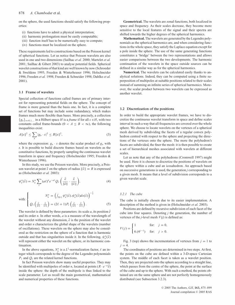
In this study, we use the Poisson wavelets. More precisely, a Pois-
son wavelet at point �x on the sphere of radius ‖�x‖ = R is expressed
as (Holschneider et al. 2003):
ψna (�x) = N n
a
∑
ℓ
(aℓ)ne−aℓ Qℓ
(
�e
‖�e‖·
�x
‖�x‖
)
, (4)
with:
N na =
(
∫
S(r )ψn
a (�x).ψna (�x)ds(�x)
)− 12
Qℓ
(
�e‖�e‖
· �x‖�x‖
)
= (2ℓ + 1)Pℓ
(
�e‖�e‖
· �x‖�x‖
)
. (5)
The wavelet is defined by three parameters: its scale a, its position �eand its order n. In other words, a is a measure of the wavelength of
the wavelet without any dimension, �e is the position of the wavelet
and order n characterizes the global shape of the wavelets (number
of oscillations). These wavelets on the sphere may also be consid-
ered as the restriction on the sphere of a function that is harmonic
outside and that has singularities inside it. In the following, ψna (�x)
will represent either the wavelet on the sphere, or its harmonic con-
tinuation.
In the above equations, Nna is a L2-normalization factor, ℓ an in-
teger which corresponds to the degree of the Legendre polynomials
Pℓ and Qℓ are the related kernel functions.
In fact Poisson wavelets show many useful properties. They may
be identified with multipoles of order n, located at points (R · e−a�e)
inside the sphere: the depth of the multipole is thus linked to the
scale parameter. Let us recall the main geometrical, mathematical
and numerical properties of these functions.
Geometrical. The wavelets are zonal functions, both localized in
space and frequency. As their scales decrease, they become more
sensitive to the local features of the signal and their spectra are
shifted towards the higher degrees of the spherical harmonics.
Mathematical. The wavelets are generated by the Legendre poly-
nomials as the spherical harmonics are, and when considering func-
tions in the whole space, they satisfy the Laplace equation except for
a pole inside the sphere. The use of the same generating functions
constitutes a ‘bridge’ between the two representations and allows
easier comparisons between the two developments. The harmonic
continuation of the wavelets in the space outside sources can be
defined in a similar way as for the spherical harmonics.
Numerical. The wavelets can be calculated easily thanks to an-
alytical solutions. Indeed, they can be computed using a finite su-
perposition of multipoles at suitable positions related to their scales
instead of summing an infinite series of spherical harmonics. More-
over, the scalar product between two wavelets can be expressed as
another wavelet.
3.2 Discretization of the positions
In order to build the appropriate wavelet frames, we have to dis-
cretize the continuous wavelet transform in space and define scales
interval in such a way that all frequencies are covered over the whole
sphere. We choose to locate wavelets on the vertexes of a spherical
mesh derived by subdividing the facets of a regular convex poly-
hedron centred with respect to the sphere and projecting the direc-
tions of the vertexes onto the sphere. The more the polyhedron’s
facets are subdivided, the finer the mesh: it is then possible to create
a set of hierarchical meshes associated with wavelets at different
scales.
Let us note that any of the polyhedrons (Cromwell 1997) might
be used. Here it is chosen to discretize the positions of wavelets on
the sphere within a cube and an icosahedron. An approach based
on successive generations is used, the generation j corresponding to
a given mesh. It means that a level of subdivision corresponds to a
given wavelet scale.
3.2.1 The cube
The cube is initially chosen due to its easier implementation. A
description of the method is given in (Holschneider et al. 2003).
Positions are defined by recursive subdivision of each facet of the
cube into four squares. Denoting j the generation, the number of
vertexes of the j-level mesh V (j) is defined as:
V ( j) =
{
1 for: j = 0,
6.(4 j−1) for: j > 0.
Fig. 3 (top) shows the incrementation of vertexes from j = 1 to
j = 4.
The coordinates of positions are determined in two steps. At first,
the points on the cube are defined within a 3-D-space Cartesian
system. The middle of each facet is taken as a wavelet position.
Then, they are projected onto the sphere according to a straight line,
which passes from the centre of the sphere, the point at the surface
of the cube and up to the sphere. With such a method, the points ob-
tained are on the same sphere and are not perfectly homogeneously
distributed (see Subsection 3.2.3).
C© 2005 The Authors, GJI, 163, 875–899
Journal compilation C© 2005 RAS

Wavelet frames: an alternative to spherical harmonic representation of potential fields 879
j = 1 j = 2 j = 3 j = 4
Figure 3. Facets of polyhedrons at each generation j for a cube (top) and
an icosahedron (bottom). Black crosses represent positions of wavelets.
3.2.2 The icosahedron
The second chosen polyhedron is the icosahedron. The description
of its implementation is given in (Kenner 1976).
Positions are defined by recursive subdivision of each facet of the
icosahedron into four triangles connecting the middle of the sides.
As for the cube, the number of vertexes of the j-level mesh is denoted
V (j):
V ( j) =
{
1 for: j = 0,
10.(4 j−1) + 2 for: j > 0.
Fig. 3 (bottom) shows the incrementation of vertexes from j = 1
to j = 4.
The coordinates of positions are determined in the same two steps
as for the cube. Nevertheless, the method is slightly different in
the sense that the vertexes defining positions are not the middle of
facets as for the cube. More interesting, the points are more regularly
distributed than for the cube.
3.2.3 Comparison of the two meshes
The number of points at each generation is depicted in Fig. 4.
The icosahedric meshes comprise more vertexes than the cubi-
cal ones: the ratio tends to about 1.7 as j increases. Moreover, at
level ( j + 1), it includes all the vertexes of level j. On the con-
trary, vertexes from the cubical meshes never coincide between
0 2 4 6
Generation j
0
1000
2000
3000
4000
5000
6000
Nu
mb
er o
f v
erte
xes
per
gen
era
tio
n V
(j)
cube
icosahedron
Generation j V(j) for the cube V(j) for the icosahedron
0 1 1
1 6 12
2 24 42
3 96 162
4 384 642
5 1536 2562
6 6144 10242
Figure 4. Number of points of the polyhedrons at each generation j.
Figure 5. Meshes on the sphere at two generations j, calculated for a cube
(top) and an icosahedron (bottom).
j and ( j + 1) generations. Both kinds of meshes (Fig. 5) show
a good regularity even if a non-negligible dispersion of distances
between points is observed. The dispersion of distances between
points at different generation for cubical and icosahedrical meshes
is roughly coming to, respectively, 30 and 10 per cent of the
mean value. This phenomenon is not significative for the resolu-
tion obtained in this study. In this paper, both kind of meshes are
used in order to provide two different examples of wavelet frame
discretization.
The regularity of the meshes is a difficult problem, known as ‘Le
probleme des dictateurs ennemis’: how to distribute territories of
sphere to several dictators so that they have all the same territory and
that they are as distant as possible from each other. The interested
reader may find more details in an abundant bibliography on the
subject (Hicks & Wheeling 1959; Muller 1959).
3.3 Discretization of the scales
In the previous subsection, we described the discretization of wavelet
positions (θ , φ) on the sphere. We have now to associate to each gen-
eration j of positions the corresponding scale aj. This last parameter
has to be carefully chosen in order to satisfy two main constraints:
(i) the spectrum should be covered and (ii) the number of wavelets
of each scale should be sufficient, but not too large, to generate the
corresponding spherical harmonics.
The sequence of the scales is defined on a unit sphere 1 and
corresponds to a geometric progression:
a j = a0 · γ j−1, (6)
where j is the generation, a0 is a chosen initial scale and γ , a constant
verifying: 0 < γ < 1.
Then, the position (r j , θ , φ)1of the corresponding multipole
inside 1 is:{
r j = e−a j
(θ, φ) given by the mesh.
C© 2005 The Authors, GJI, 163, 875–899
Journal compilation C© 2005 RAS

880 A. Chambodut et al.
The bounds of scales and of positions for ‘sources’ within 1
are:{
0 < a j ≤ a0
1 > r j ≥ e−a0
.
Considering the Earth’s surface noted E , we define new posi-
tions Rj and their associated scales Aj:
A j = a j − ln
(
Rref
RE
)
, (7)
R j = Rref · r j . (8)
RE is the mean radius of the Earth. Rref allows to introduce a priori
information in the incrementation of scale, as it corresponds to radii
of known discontinuities of the Earth. Indeed, all multipoles located
inside (resp. outside) a sphere of radius Rref have a scale parameter
greater (resp. lower) than:
Aref = − ln
(
Rref
RE
)
. (9)
Then, we can choose the scales of wavelet frames in order to sample
the desired layers of the Earth’s interiors, taking into account the a
priori structures.
The mathematical relation between Rj and Aj is the same as for
the unit sphere:
R j = RE · e−A j . (10)
In the following, we discuss two possible examples of frames to
represent magnetic and gravity data.
3.3.1 Magnetic field
For the magnetic field, we choose to implement a frame based on
the multipoles of order 2. This order allows a good coverage of low
degrees of the spherical harmonics. Moreover, it yields a precise
localization in both space and frequency. The scale aj associated to
the j-level on the unit sphere verifies a0 = 2 and γ = ( 12). Positions
(θ , φ) are discretized on the cubical mesh.
Different frames are then used for the scalar and vectorial cases.
Indeed, the demanding constraints and the physical meanings of this
last case are more important than the simple fit of a scalar function
on the sphere.
For the scalar case, the wavelets regularly sample the wavelengths
present in the modelled scalar function, which is the intensity of the
magnetic field | �B|. We thus simply use: R ref = RE. Table 1 shows the
multipole characteristics for different generations. Fig. 6 top shows
that the spectrum is covered. In the Fig. 6 bottom, we compare the
number of wavelets with the number of spherical harmonics. Each
Table 1. Sequence of scales chosen for the frame used in scalar case for
magnetic field modelling.
j aj = Aj rj Rj = rjRE (km)
1 2 0.135 860 Large scale
2 1 0.368 2345
3 0.5 0.607 3867
4 0.25 0.779 4963
5 0.125 0.883 5626
6 0.0625 0.939 5985 Small scale
0.0 1.0 6371.2 Earth’s surface
0 5 10 15 20 25 30
Degree of the spherical harmonics
0
50
100
150
2000 5 10 15 20 25 30
0
0.5
1
Sp
ectr
um
of
the w
avele
ts
Figure 6. Discretization of the scales with order 2 multipoles. The energy
spectra for the generations 1 to 6 are computed (top panel). The number
of wavelets (areas defined by thin segments) is compared to the number
of spherical harmonics (areas below thick line) for each degree ℓ (bottom
panel).
0 5 10 15 20 25 30
Degree of the spherical harmonics
0
50
100
150
2000 5 10 15 20 25 30
0
0.5
1
Sp
ectr
um
of
the w
avele
ts
Figure 7. Discretization of the scales with order 2 multipoles. The energy
spectra for the generations 1 to 5 on the core (top panel, solid curves) and 1
to 6 on the crust (top panel, dashed curves) are calculated (top). The squares
define the limit spectrum of the core-wavelets. The number of wavelets from
the core (areas defined by thick segments) and from the crust (areas defined
by thin segments) is compared to the number of spherical harmonics (areas
below thick line) for each degree ℓ (bottom panel). Note that (i) the spectra
of core-wavelets cover spherical harmonic up to degree ℓ ≃ 13; (ii) the core-
wavelets are more redundant than the crustal ones below ℓ = 13 and (iii)
only crustal-wavelets represent the field when ℓ ≥ 16.
area defined by thin segments represents the number of wavelets of a
given scale. The limits of the areas depend on the spectral coverage of
the wavelets. The wavelet spectrum has an infinite support. However,
we only consider the part retaining most of the wavelet energy. The
number of wavelets is large enough, comparing to the number of
spherical harmonics.
For the vectorial case, the positions of multipoles correspond to
the core of the Earth: R ref = RCMB = 3485 km, and to the crust:
C© 2005 The Authors, GJI, 163, 875–899
Journal compilation C© 2005 RAS

Wavelet frames: an alternative to spherical harmonic representation of potential fields 881
Table 2. Sequence of scales chosen for the frame used in vectorial case
magnetic field modelling.
j aj aj rj rj (km)
1 2 2.6 0.135 472 Core: large-scale
2 1 1.6 0.368 1282
3 0.5 1.1 0.607 2114
4 0.25 0.85 0.779 2714 Core: small scale
0.0 0.60 1.0 3485 CMB
1 2 2 0.135 860 Crust: large scale
2 1 1 0.368 2345
3 0.5 0.5 0.607 3867
4 0.25 0.25 0.779 4963
5 0.125 0.125 0.883 5626
6 0.0625 0.0625 0.939 5985 Crust: small scale
0.0 0.0 1.0 6371.2 Earth’s surface
R ref = RE = 6371.2 km. Table 2 shows the multipole characteristics
for different generations.
Fig. 7 shows that the spectrum is covered, and that the number
of wavelets is large enough compared to the number of spherical
harmonics. The core and crustal wavelets cover all the spherical
harmonic degrees. Indeed, it is necessary even for low degrees to
consider both fields as the synthetic data in spherical harmonics do
not distinguish the two contributions. In an ideal case, with an infi-
nite number of wavelets, it would be possible to consider a wavelet
model with positions of multipoles that would purely correspond
to physical sources (for example: R crust ≥ 6341.2 km → Acrust ≤0.005). The radial positions of the wavelets inside the Earth, noted
Rj in Table 2, are given as an equivalent representation by using the
non-unicity of the solution given by wavelet frames. Thus, the Rj
constitute the positions of equivalent sources.
3.3.2 Gravity field
For the gravity field, we choose to implement a frame based on
order 3 multipoles. The localization in space and frequency is still
satisfactory: indeed, the wavelets only show one spatial undulation
and their spectra narrow. Let us notice that the spectra of these
wavelets shift towards the higher degrees and show less power in the
lower degrees. Choosing a frame based on higher order multipoles
would degrade the spatial localization of the wavelets.
The scale associated to the j-level verifies a0 = 3 and γ = 12. The
sequence of multipole depths Rj inside the Earth, regularly sam-
ples its successive concentric envelops, to reflect the distribution
of masses: R ref = R Eeq = 6378.1 km. Table 3 shows the multipole
Table 3. Sequence of scales chosen for the frame used in gravity modelling.
j aj = Aj Rj = rjRE (km) Location
1 3 318 Inner core
2 1.5 1423 Outer core
3 0.75 3013 Outer core
4 0.375 4384 Lower mantle
5 0.1875 5288 Lower mantle
6 0.09375 5807 Upper mantle
7 0.046875 6086 Upper mantle
8 0.023438 6230 Upper mantle
9 0.011719 6304 Upper mantle (lithosphere)
10 0.005859 6341 Crust
0.0 6378.1 Earth’s surface
0 20 40 60 80 100
Degree of the spherical harmonics
0
200
400
600
800
0 20 40 60 80 1000
0.5
1
Sp
ec
tru
m o
f th
e w
av
ele
ts
Figure 8. Discretization of the scales with order 3 multipoles. The energy
spectra for the generations 1 to 7 are calculated (top panel). The number
of wavelets (areas defined by thin segments) is compared to the number
of spherical harmonics (areas below thick line) for each degree ℓ (bottom
panel).
depths for different generations. Those multipoles are considered as
equivalent sources when modelling the disturbing potential (vecto-
rial case, see Section 4).
Positions (θ , φ) are discretized on the icosahedric meshes since
the gravity anomalies are modelled at a rather high resolution.
Fig. 8 shows that the spectrum is homogeneously covered, and that
the number of wavelets is large enough as compared to the number of
spherical harmonics. Let us notice that this frame is more redundant
than the other one on the cube.
4 I N V E R S E P RO B L E M
4.1 The least-squares method
The magnetic and gravity fields (resp. �B and �g) can be expressed as
a linear combination of wavelets. In the following, we are focusing
on the two quantities used by magnetic and gravity communities:
the magnetic field and the free air gravity anomaly.1 In the scalar
case, the intensity of magnetic field and gravity anomaly are directly
written as a sum of wavelets. In the vectorial case, only potentials
are expressed as a sum of wavelets modelled as superposition of
multipolar potentials. Thereafter, the magnetic field and the gravity
anomaly are derived.
Denoting E the function to be represented, α the vector of wavelet
coefficients and ψ the wavelet frame, the following general equality
holds :
E =∑
i
αiψi (11)
1The free air gravity anomaly is defined as the difference between the in-
tensity of the real gravity field at the point of measurement and the intensity
of the normal gravity field at the same point: the resulting value is called
the ‘gravity disturbance’ among the geodetic community, but here it will be
called ‘gravity anomaly’. It can be linked to the disturbing potential T , which
is defined as the difference between the real gravity potential of the Earth
and the normal potential of the reference ellipsoid (Moritz 1989; Hackney
& Featherstone 2003).
C© 2005 The Authors, GJI, 163, 875–899
Journal compilation C© 2005 RAS
882 A. Chambodut et al.
In order to find the coefficients α i of the wavelet development,
we set a classical least-squares problem. This method consists in
deriving the set of coefficients, which minimizes the residuals be-
tween the data and the model in a L2 sense. However, many sets of
coefficients lead to a good fit of the data since the problem is of-
ten underdetermined. Thus, we have to take into account additional
constraints in order to eliminate the overfitted solutions that show
large oscillations. Here, we introduced a smoothness constraint to
regularize the problem. However, the smoother the solution is, the
worse the measurement residuals are: we have to find a trade-off
between a good fit of data and the global smoothness. We actually
minimize the following quantity:
(b − Mα)t · W · (b − Mα) + λαt · L · α (12)
leading to the normal system:
(M t · W · M + λL) · α = M t · W · b, (13)
where b is the vector of measurements. M is a (i × j) matrix. The
jth column of the matrix M contains the jth wavelet sampled at the
i observation points. α is the vector of wavelet coefficients; W is a
matrix of data weighting; L is the matrix of a quadratic form that
controls the regularity, and λ is a parameter balancing between fit
and smoothness. The parameter λ has to be chosen in such a way
that, on the one hand, it avoids the model to fit the data with a
precision better than their noise (case of overfitting, for which the
solution is too oscillating). On the other hand, it avoids the case of
underfitting, for which the solution is too smooth.
Eq. (13) is actually related to the general theory of inverse prob-
lems (see for instance Tarantola 1987). In this theory, on the one
hand, we suppose that the observation errors have a Gaussian distri-
bution with covariance matrix W −1. On the other hand, the a priori
probability of a model, of a set of coefficients α, is again a Gaussian
distribution with density exp(−λ (αt ·L · α)) where L is the matrix
of a bilinear quadratic form. Typically, L describes how the field en-
ergy decreases from the large scales to the small ones: coefficients
at large scales show indeed larger variances than those at small
scales.
Measurements bring additional information, so that an a poste-
riori probability on the coefficients can be computed, taking the
measurements as well as the a priori knowledge into account. The
vector of coefficients for which this a posteriori probability reaches
a maximum is given by eq. (13).
In the following, we assume an uncorrelated noise on the data, so
W is diagonal with:
Wi j =1
σ 2j
· δi j , (14)
where σ 2j is the variance of the noise of jth measurement. When
measurements are very precise, the diagonal terms of W become
very large, implying a stronger constraint on measurement residuals.
We provide two examples of regularization, keeping in mind the
notion of spectral decrease.
We now detail eq. (13) for both scalar and vectorial cases.
4.2 Scalar case
In the scalar case, the function E (eq. 11) represents the intensity of
the magnetic field | �B| or the gravity anomaly �g. Thus, b is directly
the vector of measurements of | �B| or �g.
Studying the scalar case is mainly a way to check the applicability
of the method rather than to get a representation of potential fields.
It allows us to apprehend the behaviour of the wavelets and the
influence of each parameter of the model (incrementations of scales,
discretizations of positions, choices of the regularization parameter
λ). The scalar case also allows to test the capability of the wavelets
to represent a given function E on the sphere.
An important task is how to define the L matrix. In the following,
we present two examples in how it can be chosen. The first example
is mainly applied to the magnetic field and the second to the gravity
field. However, it is possible to exchange the presented approaches
between the two fields.
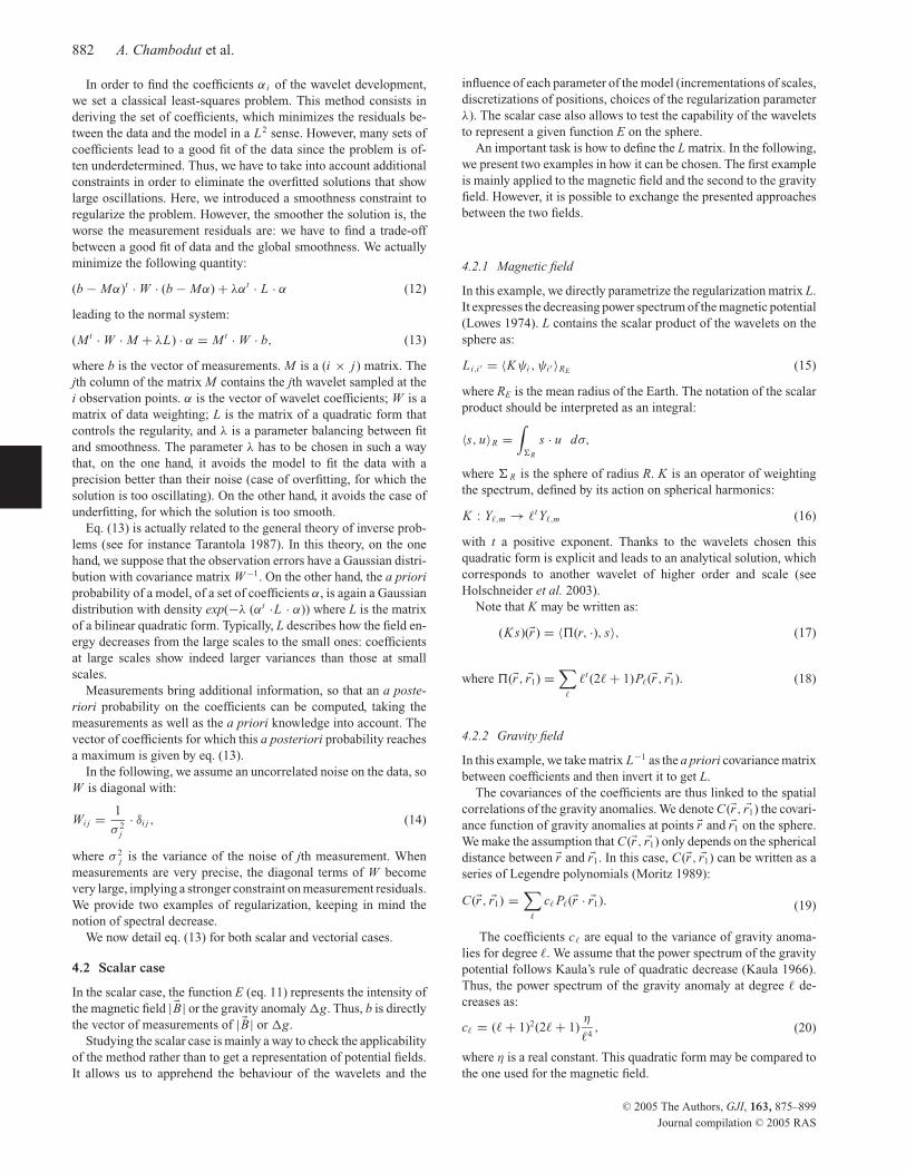
4.2.1 Magnetic field
In this example, we directly parametrize the regularization matrix L.
It expresses the decreasing power spectrum of the magnetic potential
(Lowes 1974). L contains the scalar product of the wavelets on the
sphere as:
L i,i ′ = 〈Kψi , ψi ′ 〉RE(15)
where RE is the mean radius of the Earth. The notation of the scalar
product should be interpreted as an integral:
〈s, u〉R =
∫
R
s · u dσ,
where R is the sphere of radius R. K is an operator of weighting
the spectrum, defined by its action on spherical harmonics:
K : Yℓ,m → ℓt Yℓ,m (16)
with t a positive exponent. Thanks to the wavelets chosen this
quadratic form is explicit and leads to an analytical solution, which
corresponds to another wavelet of higher order and scale (see
Holschneider et al. 2003).
Note that K may be written as:
(K s)(�r ) = 〈�(r, ·), s〉, (17)
where �(�r , �r1) =∑
ℓ
ℓt (2ℓ + 1)Pℓ(�r , �r1). (18)
4.2.2 Gravity field
In this example, we take matrix L−1 as the a priori covariance matrix
between coefficients and then invert it to get L.
The covariances of the coefficients are thus linked to the spatial
correlations of the gravity anomalies. We denote C(�r , �r1) the covari-
ance function of gravity anomalies at points �r and �r1 on the sphere.
We make the assumption that C(�r , �r1) only depends on the spherical
distance between �r and �r1. In this case, C(�r , �r1) can be written as a
series of Legendre polynomials (Moritz 1989):
C(�r , �r1) =∑
ℓ
cℓ Pℓ(�r · �r1). (19)
The coefficients cℓ are equal to the variance of gravity anoma-
lies for degree ℓ. We assume that the power spectrum of the gravity
potential follows Kaula’s rule of quadratic decrease (Kaula 1966).
Thus, the power spectrum of the gravity anomaly at degree ℓ de-
creases as:
cℓ = (ℓ + 1)2(2ℓ + 1)η
ℓ4, (20)
where η is a real constant. This quadratic form may be compared to
the one used for the magnetic field.
C© 2005 The Authors, GJI, 163, 875–899
Journal compilation C© 2005 RAS

Wavelet frames: an alternative to spherical harmonic representation of potential fields 883
Let us now denote K the operator associating to each square
integrable function on the sphere f its scalar product with C(�r , �r1):
(K f )(�r ) = 〈C(�r , ·), f 〉REeq, (21)
where REeq is the mean equatorial radius of the Earth. We derive the
covariance between two coefficients α i and α i ′ as a scalar product
between the corresponding wavelets. This comes from the formulae
of covariance propagation by (Moritz 1989):
L−1i,i ′
= 〈Kψi , ψi ′ 〉REeq. (22)
The last step consists in inverting the matrix given by eq. (22) to get
L.
4.3 Vectorial case
In the vectorial case, the function E represents the magnetic po-
tential VM or the gravity disturbing potential T (see footnote 1 in
Section 4.1).
The measurement vector b contains no values of VM or T , but the
vectorial components of the magnetic field or the gravity anomaly in
the radial spherical approximation (the gravity anomaly is a scalar
but in the spherical approximation, it is oriented in the radial direc-
tion and then considered here as vectorial). Thus the matrix M is
different for each inverse problem. Sections 4.3.1 and 4.3.2 present
the equation systems for the two fields.
4.3.1 Magnetic field
The magnetic field is represented via a superposition of the deriva-
tives of the wavelets in the spherical coordinate system :
�B =
Br
Bθ
Bφ
=
− ∂V
∂r
− 1r
∂V
∂θ
− 1r sin θ
∂V
∂φ
, (23)
�B =∑
i
αi
− ∂ψi
∂r
− 1r
∂ψi
∂θ
− 1r sin θ
∂ψi
∂φ.
(24)
In matricial notation, eq. (24) becomes:
�B = M.α (25)
The L matrix is, as for the scalar case, chosen in order to allow
a balance between a good fit and a global smoothness. We choose
to implement it in order to assume a regularity on the potential
through constraint on Br the radial component of the magnetic field.
Thus:
L i,i ′ =
⟨
∂
∂rψi ,
∂
∂rψi ′
⟩
RE or RC M B
. (26)
The value of the radial derivative increases when the scale decreases.
Thus, small-scale wavelets are more expensive than large-scale ones.
This matrix is applied on both groups of wavelets supposed to rep-
resent the core and the lithosphere.
4.3.2 Gravity field
In the spherical approximation, the free air gravity anomaly is related
to the disturbing potential Moritz (1989):
�g = −∂T
∂r, (27)
where r is the spherical radius. The wavelet expansion of the gravity
anomaly is then derived by linearity:
�g = −∑
i
αi
(
∂ψi
∂r
)
. (28)
In matricial notation, eq. (28) becomes:
�g = M.α (29)
As for the scalar case, the matrix L is defined as the inverse of the
covariance matrix of the wavelet coefficients, but these coefficients
correspond now to the wavelet approximation of the disturbing po-
tential. This matrix is derived in the same way as described in Sec-
tion 4.2.2. However, the power spectrum of the gravity anomalies
has to be replaced by the power spectrum of the disturbing potential.
The Kaula’s rule for the potential reads :
cℓ = (2ℓ + 1)β
ℓ4, (30)
where β is a real constant.
5 R E S U LT S
In the present paper, we only discuss tests obtained from synthetic
data sets. Indeed, this choice allows: (1) to know exactly the spatial
and spectral contents of the used information, (2) to test as many
distributions of data as possible and (3) to directly compare with
the initial model in spherical harmonics. The two fields, magnetic
and gravity, differ in their spatial and spectral characteristics. Their
behaviours help us to study the impact of different parameters of the
used wavelet frames.
The results we obtained are presented for magnetic and grav-
ity fields, separately. Moreover, we made a distinction between the
global and regional representations, obtained with both possible reg-
ular and irregular distributions.
5.1 Magnetic models
5.1.1 Global representations
Data. We used a synthetic data set computed from the CO2 model
(Holme et al. 2003). This model is obtained from the measurements
27500 33000 38500 44000 49500 55000 60500 66000
|B| (nT)
Figure 9. Map for the magnetic field intensity (| �B|) computed at the Earth’s
surface, from CO2 model (Holme et al. 2003) up to degree/order 13. Black
dots represent the chosen irregular distribution of data, which directly cor-
respond to the distribution of 670, past and present, magnetic observatory
locations.
C© 2005 The Authors, GJI, 163, 875–899
Journal compilation C© 2005 RAS

884 A. Chambodut et al.
-14500 -7250 0 7250 14500 21750 29000 36250
X (nT)
-16748 -12561 -8374 -4187 0 4187 8374 12561
Y (nT)
-63648 -47736 -31824 -15912 0 15912 31824 47736
Z (nT)
Figure 10. Same as Fig. 9 for Northern X (top), Eastern Y (middle) and
Downward vertical Z (bottom) components.
Table 4. Parameters of the global tests—magnetic scalar case.
Parameters Regular case Irregular case
(629 data) (670 data)
Order of multipoles 2 2
Generations of the frame 1 to 4 1 to 4
Scales See Table 1 See Table 1
Number of wavelets 510 510
W matrix 1I 1I
λ parameter 10−10 10−9
t exponent parameter 7 7
provided by three magnetic satellites: CHAMP, Ørsted and SAC-
C, from 2000 August to 2001 December. This spherical harmonic
model is developed up to degree/order 29 when describing the in-
ternal field. The magnetic field spectrum is clearly decreasing up to
degree/order 13 (Fig. 1). We truncated the CO2 model at this degree,
Table 5. Parameters of the global tests—magnetic vectorial case.
Parameters Regular case Irregular case
(629 data) (670 data)
Wavelets belong to: Core/crust Core/crust
Order of multipoles 2/2 2/2
Generations of the frame 1 to 4/1 to 3 1 to 3/1 to 3
Scales See Table 2 See Table 2
Number of wavelets 510/126 126 /126
W matrix 1I 1I
λ parameter 10−21 10−14
-1800 -1350 -900 -450 0 450 900 1350 1800
δ|B| (nT)
Figure 11. Map of residuals on the magnetic field intensity (| �B|) at the
Earth’s surface (initial spherical harmonic model CO2 – 510 wavelet model).
The wavelet model is computed applying the scalar case on the regular
distribution of 629 data.
−1000 −800 −600 −400 −200 0 200 400 600 800 1000
Values of residuals (nT)
0
5
10
15
Fre
qu
en
cy
(%
)
Figure 12. Histograms of residuals on the magnetic field intensity | �B|(initial synthetic data from spherical harmonics model CO2—reconstructed
data from 510 wavelet model). The wavelet model is computed applying the
scalar case on the regular distribution of 629 data.
for global representations of main internal contributions (Figs 9 and
10).
From this model, we constituted a regular and an irregular dis-
tribution of data. We did not apply a Gaussian filter on synthetic
data as it was done for gravity modelling (see below). The regu-
lar distribution of synthetic data comprises 629 samples, with one
data per bin of 10◦ × 10◦ on the whole Earth’s surface. The irreg-
ular distribution contains 670 samples, located at all observatory
C© 2005 The Authors, GJI, 163, 875–899
Journal compilation C© 2005 RAS

Wavelet frames: an alternative to spherical harmonic representation of potential fields 885
-1.0 -0.5 0.0 0.5 1.0
δX (nT)
-1.0 -0.5 0.0 0.5 1.0
δY (nT)
-1.0 -0.5 0.0 0.5 1.0
δZ (nT)
Figure 13. Maps of residuals on the magnetic field Northern X (top), East-
ern Y (middle) and Downward vertical Z (bottom) components at the Earth’s
surface (initial spherical harmonic model CO2 – 636 wavelet model). The
wavelet model is computed applying the vectorial case on the regular distri-
bution of 629 data.
positions that have ever run on the Earth (past and present observa-
tory locations). We chose this realistic distribution because it allows
to get dense (Europe) and sparse (Pacific) covered areas.
Tests. Tables 4 and 5 summarize the parameters used in global
magnetic field modelling. We fixed a noise level at 1 nT for all
tests presented below: matrix W is thus set to the identity matrix
in all computations. This choice is motivated by the fact that data
are supposed to be ‘perfect’. The order of multipoles, the number
of generations of the frame and the scale sequences are fixed with
respect to some geophysical constraints (see paragraph 3.3.1). Thus
the residuals between the synthetic data and their wavelet repre-
sentation are minimized by adjusting the following parameters: the
exponent of regularization t in the scalar case, the quadratic form
(matrix L) in the vectorial case and the regularization parameter λ
in both cases.
−1 −0.5 0 0.5 1
Values of residuals (nT)
05
10152025
Fre
qu
en
cy (
%)
−1 −0.5 0 0.5 10
10
20
−1 −0.5 0 0.5 105
10152025
X
Y
Z
Figure 14. Histograms of residuals on the magnetic field vectorial com-
ponents (initial synthetic data from spherical harmonic model CO2—
reconstructed data from 636 wavelet model). The wavelet model is computed
applying the vectorial case on the regular distribution of 629 data.
27500 33000 38500 44000 49500 55000 60500 66000
|B| (nT)
Figure 15. Map for the magnetic field intensity (| �B|) computed at the
Earth’s surface from 510 wavelet model. Black dots represent the chosen
irregular distribution of 670 synthetic data used in the scalar case.
Results—regular case. The obtained wavelet models are not
mapped here. Indeed, they mimic the initial synthetic data provided
by CO2 model (Figs 9 and 10). For the scalar case, the residuals
between the CO2 and the wavelet models (Fig. 11) are rather impor-
tant, up to ±1800 nT. Nevertheless, the residuals between the initial
synthetic and reconstructed data (Fig. 12) are well centred on zero
and reach limits of ±400 nT. The scalar case is presented just as a
simple fit of the data: the regularization is rough and it is not based
on geophysical considerations.
The results obtained for the vectorial case show the real advan-
tages when applying the wavelets. First of all, the residuals between
the CO2 and the wavelet models (Fig. 13) are smaller than the con-
sidered noise of 1 nT. Furthermore, the residuals between initial
synthetic and reconstructed data (Fig. 14) are well centred on zero,
being no larger than ±0.25 nT. Due to the number and the reparti-
tion of data, low regularizations (see λ parameter in Tables 5) allow
an easy recovery of the initial spherical harmonic model up to de-
gree/order 13.
Results—irregular case. Fig. 15 shows a map of the intensity
of the magnetic field modelled by wavelets. When comparing with
Fig. 9, one can see additional oscillations, without major changes
on the global shape of the intensity. The residuals between the CO2
and the wavelet models (Fig. 16) reach some huge values, up to
−10 000 nT in the South Atlantic area or 5000 nT in India Ocean.
C© 2005 The Authors, GJI, 163, 875–899
Journal compilation C© 2005 RAS

886 A. Chambodut et al.
-9000 -7500 -6000 -4500 -3000 -1500 0 1500 3000 4500
δ|B| (nT)
Figure 16. Map of residuals on the magnetic field intensity (| �B|) at the
Earth’s surface (initial spherical harmonic model CO2 – 510 wavelet model).
The wavelet model is computed applying the scalar case on the irregular
distribution of 670 data.
−500 −300 −100 100 300 500
Values of residuals (nT)
0
5
10
15
20
Fre
qu
en
cy
(%
)
Figure 17. Histograms of residuals on the magnetic field intensity | �B|(initial synthetic data from spherical harmonics model CO2—reconstructed
data from 510 wavelet model). The wavelet model is computed applying the
scalar case on the irregular distribution of 670 data.
In this case, the residuals on the data (Fig. 17) vary up to ±300 nT.
This model points out the key role of the regularization. Indeed, the
small-scale wavelets are not sufficiently constrained. If the regular-
ization parameter λ is increasing, the resolution decreases, leading
to an increase of the residuals on the data. If λ is decreasing, the
residuals also decrease up to ±5 nT but the obtained model is less
regular. Fig. 18 shows maps for X , Y and Z magnetic field compo-
nents modelled by wavelets. When comparing these maps with those
shown in Fig. 10, no remarkable differences appear between the ini-
tial spherical harmonic and the wavelet models. For all regions well
covered by data the residuals for all three components are as small
as a few tens of nT. As expected, the largest residuals (Fig. 19) are
in areas without data (Pacific Ocean, Southern Atlantic region). For
regions without data, these residuals are larger. These differences
are due to the spherical harmonic model, as wavelet model does not
introduce spurious artefacts when data are missing. Let us empha-
size that a recalculated spherical harmonic model from the same
data set represents these data in a less accurate way than the wavelet
model we presented here. The residuals on data (Fig. 20) are larger
-14500 -7250 0 7250 14500 21750 29000 36250
X (nT)
-16748 -12561 -8374 -4187 0 4187 8374 12561
Y (nT)
-63648 -47736 -31824 -15912 0 15912 31824 47736
Z (nT)
Figure 18. Maps for the magnetic field Northern X (top), Eastern Y (mid-
dle) and Downward vertical Z (bottom) components computed at the Earth’s
surface from 252 wavelet model. Black dots represent the chosen irregular
distribution of 670 synthetic data used in the vectorial case.
than for the regular case up to ±25 nT. These last results were ob-
tained with an increased regularization parameter. We had to choose
a trade-off between a regular field at Earth’s surface and a reasonable
fit of data. Again, decreasing the regularization parameter λ up to
1 · 10−21 leads to a better fit of initial data, with residuals no larger
than ±10 nT.
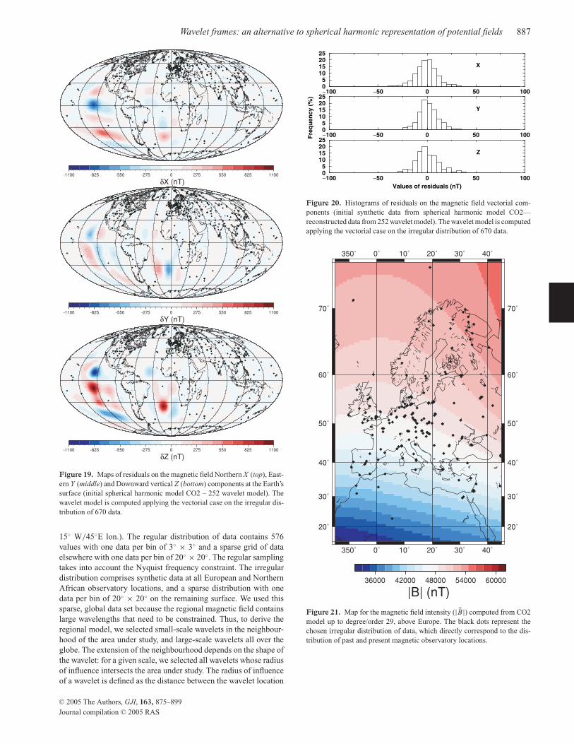
5.1.2 Regional representation
Data. For the regional representation we chose an area centred over
Europe, as it contains the largest number of magnetic observato-
ries. The intensity | �B| and the three components X , Y and Z of the
magnetic field computed up to degree/order 29 from the CO2 model
centred over the considered area are shown in Figs (21) and (22).
From the same model, we also computed an regular and an ir-
regular distribution of data centred over Europe (15◦ N/75◦ N lat.;
C© 2005 The Authors, GJI, 163, 875–899
Journal compilation C© 2005 RAS
Wavelet frames: an alternative to spherical harmonic representation of potential fields 887
-1100 -825 -550 -275 0 275 550 825 1100
δX (nT)
-1100 -825 -550 -275 0 275 550 825 1100
δY (nT)
-1100 -825 -550 -275 0 275 550 825 1100
δZ (nT)
Figure 19. Maps of residuals on the magnetic field Northern X (top), East-
ern Y (middle) and Downward vertical Z (bottom) components at the Earth’s
surface (initial spherical harmonic model CO2 – 252 wavelet model). The
wavelet model is computed applying the vectorial case on the irregular dis-
tribution of 670 data.
15◦ W/45◦E lon.). The regular distribution of data contains 576
values with one data per bin of 3◦ × 3◦ and a sparse grid of data
elsewhere with one data per bin of 20◦ × 20◦. The regular sampling
takes into account the Nyquist frequency constraint. The irregular
distribution comprises synthetic data at all European and Northern
African observatory locations, and a sparse distribution with one
data per bin of 20◦ × 20◦ on the remaining surface. We used this
sparse, global data set because the regional magnetic field contains
large wavelengths that need to be constrained. Thus, to derive the
regional model, we selected small-scale wavelets in the neighbour-
hood of the area under study, and large-scale wavelets all over the
globe. The extension of the neighbourhood depends on the shape of
the wavelet: for a given scale, we selected all wavelets whose radius
of influence intersects the area under study. The radius of influence
of a wavelet is defined as the distance between the wavelet location
−100 −50 0 50 100
Values of residuals (nT)
05
10152025
Fre
qu
en
cy (
%)
−100 −50 0 50 10005
10152025
−100 −50 0 50 10005
10152025
X
Y
Z
Figure 20. Histograms of residuals on the magnetic field vectorial com-
ponents (initial synthetic data from spherical harmonic model CO2—
reconstructed data from 252 wavelet model). The wavelet model is computed
applying the vectorial case on the irregular distribution of 670 data.
350˚
350˚
0˚
0˚
10˚
10˚
20˚
20˚
30˚
30˚
40˚
40˚
20˚ 20˚
30˚ 30˚
40˚ 40˚
50˚ 50˚
60˚ 60˚
70˚ 70˚
36000 42000 48000 54000 60000
|B| (nT)
Figure 21. Map for the magnetic field intensity (| �B|) computed from CO2
model up to degree/order 29, above Europe. The black dots represent the
chosen irregular distribution of data, which directly correspond to the dis-
tribution of past and present magnetic observatory locations.
C© 2005 The Authors, GJI, 163, 875–899
Journal compilation C© 2005 RAS
888 A. Chambodut et al.
350˚
350˚
0˚
0˚
10˚
10˚
20˚
20˚
30˚
30˚
40˚
40˚
20˚ 20˚
30˚ 30˚
40˚ 40˚
50˚ 50˚
60˚ 60˚
70˚ 70˚
6800 13600 20400 27200 34000
X (nT)
350˚
350˚
0˚
0˚
10˚
10˚
20˚
20˚
30˚
30˚
40˚
40˚
20˚ 20˚
30˚ 30˚
40˚ 40˚
50˚ 50˚
60˚ 60˚
70˚ 70˚
-6000 -4000 -2000 0 2000 4000
Y (nT)
350˚
350˚
0˚
0˚
10˚
10˚
20˚
20˚
30˚
30˚
40˚
40˚
20˚ 20˚
30˚ 30˚
40˚ 40˚
50˚ 50˚
60˚ 60˚
70˚ 70˚
10200 20400 30600 40800 51000
Z (nT)
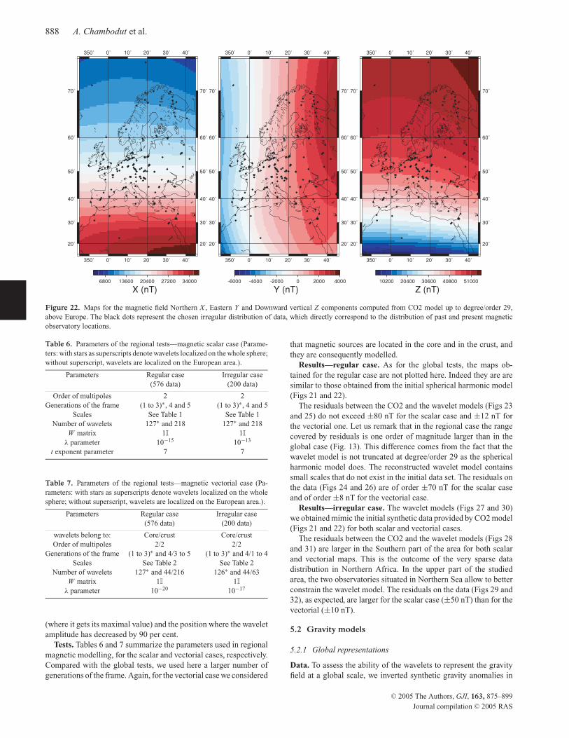
Figure 22. Maps for the magnetic field Northern X , Eastern Y and Downward vertical Z components computed from CO2 model up to degree/order 29,
above Europe. The black dots represent the chosen irregular distribution of data, which directly correspond to the distribution of past and present magnetic
observatory locations.
Table 6. Parameters of the regional tests—magnetic scalar case (Parame-
ters: with stars as superscripts denote wavelets localized on the whole sphere;
without superscript, wavelets are localized on the European area.).
Parameters Regular case Irregular case
(576 data) (200 data)
Order of multipoles 2 2
Generations of the frame (1 to 3)∗, 4 and 5 (1 to 3)∗, 4 and 5
Scales See Table 1 See Table 1
Number of wavelets 127∗ and 218 127∗ and 218
W matrix 1I 1I
λ parameter 10−15 10−13
t exponent parameter 7 7
Table 7. Parameters of the regional tests—magnetic vectorial case (Pa-
rameters: with stars as superscripts denote wavelets localized on the whole
sphere; without superscript, wavelets are localized on the European area.).
Parameters Regular case Irregular case
(576 data) (200 data)
wavelets belong to: Core/crust Core/crust
Order of multipoles 2/2 2/2
Generations of the frame (1 to 3)∗ and 4/3 to 5 (1 to 3)∗ and 4/1 to 4
Scales See Table 2 See Table 2
Number of wavelets 127∗ and 44/216 126∗ and 44/63
W matrix 1I 1I
λ parameter 10−20 10−17
(where it gets its maximal value) and the position where the wavelet
amplitude has decreased by 90 per cent.
Tests. Tables 6 and 7 summarize the parameters used in regional
magnetic modelling, for the scalar and vectorial cases, respectively.
Compared with the global tests, we used here a larger number of
generations of the frame. Again, for the vectorial case we considered
that magnetic sources are located in the core and in the crust, and
they are consequently modelled.
Results—regular case. As for the global tests, the maps ob-
tained for the regular case are not plotted here. Indeed they are are
similar to those obtained from the initial spherical harmonic model
(Figs 21 and 22).
The residuals between the CO2 and the wavelet models (Figs 23
and 25) do not exceed ±80 nT for the scalar case and ±12 nT for
the vectorial one. Let us remark that in the regional case the range
covered by residuals is one order of magnitude larger than in the
global case (Fig. 13). This difference comes from the fact that the
wavelet model is not truncated at degree/order 29 as the spherical
harmonic model does. The reconstructed wavelet model contains
small scales that do not exist in the initial data set. The residuals on
the data (Figs 24 and 26) are of order ±70 nT for the scalar case
and of order ±8 nT for the vectorial case.
Results—irregular case. The wavelet models (Figs 27 and 30)
we obtained mimic the initial synthetic data provided by CO2 model
(Figs 21 and 22) for both scalar and vectorial cases.
The residuals between the CO2 and the wavelet models (Figs 28
and 31) are larger in the Southern part of the area for both scalar
and vectorial maps. This is the outcome of the very sparse data
distribution in Northern Africa. In the upper part of the studied
area, the two observatories situated in Northern Sea allow to better
constrain the wavelet model. The residuals on the data (Figs 29 and
32), as expected, are larger for the scalar case (±50 nT) than for the
vectorial (±10 nT).
5.2 Gravity models
5.2.1 Global representations
Data. To assess the ability of the wavelets to represent the gravity
field at a global scale, we inverted synthetic gravity anomalies in
C© 2005 The Authors, GJI, 163, 875–899
Journal compilation C© 2005 RAS

Wavelet frames: an alternative to spherical harmonic representation of potential fields 889
350˚
350˚
0˚
0˚
10˚
10˚
20˚
20˚
30˚
30˚
40˚
40˚
20˚ 20˚
30˚ 30˚
40˚ 40˚
50˚ 50˚
60˚ 60˚
70˚ 70˚
-80 -40 0 40 80
δ|B| (nT)
Figure 23. Map of residuals on the magnetic field intensity (| �B|) at the
Earth’s surface (initial spherical harmonic model CO2 – 345 wavelet model).
The wavelet model is computed applying the scalar case on the regular
distribution of 576 data.
both cases of regular and irregular distribution of data. We con-
structed the synthetic data sets using the first gravity model based
on GRACE data: GGM01S Tapley et al. (2004). This model was
established with 111 days of GRACE measurements, from 2002
April to November, and is developed up to degree and order 120.
We truncated the gravity anomaly model at degree and order 12,
and applied a Gaussian filter to the spherical harmonic coefficients
in order to avoid artificial oscillations Sandwell & Renkin (1988).
The applied filter is given by:
w(ℓ) = e− (l−2)2
2(σ−2)2 , (31)
where ℓ is the degree of the spherical harmonics. We chose σ = 7.
This value corresponds to a characteristic attenuation of around 0.6.
From this model, we computed a regular and an irregular distribu-
tion of data. The regular distribution comprises 1106 samples, with
one data per bin of 7.5◦ × 7.5◦ on the whole Earth’s surface. The
7.5◦ interval was chosen in order to respect the Nyquist frequency
constraint for the degree 12. The irregular distribution comprises 99
samples, with large gaps at low latitudes and areas of higher con-
centration. We chose an arbitrary distribution of data, without any
preference for the continental areas. Indeed, gravity data are avail-
−100 −50 0 50 100
Values of residuals (nT)
0
5
10
15
Fre
qu
en
cy
(%
)
Figure 24. Histograms of residuals on the magnetic field intensity | �B|(initial synthetic data from spherical harmonic model CO2—reconstructed
data from 345 wavelet model). The wavelet model is computed applying the
scalar case on the regular distribution of 576 data.
able all over the Earth: ground-based measurements are numerous
over continents, and satellite altimetry provides a complete coverage
of the oceans.
Fig. 33 shows the gravity anomaly model GGM01S filtered as
previously explained, with the irregular distribution of data super-
imposed.
Tests. Table 8 summarizes the parameters used in gravity mod-
elling at a global scale. Parameters are the same for both scalar and
vectorial cases. We did not use the first generation of the frame: in-
deed, gravity anomalies have no component on the degrees 0 and 1
whereas the spectrum of the first generation is centred onto
degree 1.
As the data are ‘perfect’ (we did not spoil them with any syn-
thetic noise), matrix W of data weighting is arbitrary. The uni-
form weighting applied corresponds to an arbitrary data noise of
10−2 mGal for the irregular distribution of data, and 10−5 mGal for
the regular one.
Lastly, we filtered the wavelet model in the same way as the gravity
model, to insure their consistency. Indeed, real gravity anomalies,
modelled as a sum of wavelets, have an infinite spectrum. In our
examples, the synthetic data only constrain the low-frequency part:
thus, they only give an access to the low-frequency part of the wavelet
representation. The presented results are thus derived on a filtered
wavelet frame.
Results—regular case. Wavelets succeed in representing the low
harmonics of the gravity anomaly model. We do not show the wavelet
models since there is visually no difference with the GGM01S model
shown on Fig. 33.
The residuals between the initial GGM01S gravity anomaly
model and the wavelet reconstruction from an regular distribution
of data are of same magnitude as the data noise (Figs 34 and 36).
Moreover, their aspect is rather isotropic. Measurement residuals
(Figs 35 and 37) reach 5 · 10−5 mGal: same order as the 10−5 mGal
of assumed data noise.
Results—irregular case. Wavelet models obtained for the scalar
and vectorial cases (Figs 38 and 41) show that the wavelets well
handle the gaps in the data set: the wavelet model reproduces the
C© 2005 The Authors, GJI, 163, 875–899
Journal compilation C© 2005 RAS

890 A. Chambodut et al.
350˚
350˚
0˚
0˚
10˚
10˚
20˚
20˚
30˚
30˚
40˚
40˚
20˚ 20˚
30˚ 30˚
40˚ 40˚
50˚ 50˚
60˚ 60˚
70˚ 70˚
-12 -6 0 6 12
δ X (nT)
350˚
350˚
0˚
0˚
10˚
10˚
20˚
20˚
30˚
30˚
40˚
40˚
20˚ 20˚
30˚ 30˚
40˚ 40˚
50˚ 50˚
60˚ 60˚
70˚ 70˚
-12 -6 0 6 12
δ Y (nT)
350˚
350˚
0˚
0˚
10˚
10˚
20˚
20˚
30˚
30˚
40˚
40˚
20˚ 20˚
30˚ 30˚
40˚ 40˚
50˚ 50˚
60˚ 60˚
70˚ 70˚
-12 -6 0 6 12
δ Z (nT)
Figure 25. Maps of residuals on the magnetic field Northern X (left), Eastern Y (middle) and Downward vertical Z (right) components at the Earth’s surface
(initial spherical harmonic model CO2 – 387 wavelet model). The wavelet model is computed applying the vectorial case on the regular distribution of 576
data.
−20 −10 0 10 20
Values of residuals (nT)
0
5
10
15
20
Fre
qu
en
cy
(%
)
−20 −10 0 10 200
5
10
15
20−20 −10 0 10 20
0
5
10
15
20
X
Y
Z
Figure 26. Histograms of residuals on the magnetic field vectorial com-
ponents (initial synthetic data from spherical harmonic model CO2—
reconstructed data from 387 wavelet model). The wavelet model is computed
applying the vectorial case on the irregular distribution of 576 data.
main structures of the gravity anomaly model even in poorly con-
strained areas. Residuals between wavelet and GGM01S models
increase in the equatorial area, due to the large gaps in the spatial
coverage of the irregular data set (Figs 39 and 42): the wavelets
nicely predict the features in the gaps, but their amplitudes and lo-
calization are not perfect because of lack of constraints. Moreover,
spherical harmonics would lead to strong oscillations with such a
distribution of data, a phenomenon that the wavelets avoid. Let us
notice that the number of measurements is much smaller than the
number of wavelets: that is the reason why residuals can be high.
However, in areas of higher density of data, residuals do not ex-
ceed 1 mGal. Residuals between measurements and reconstructed
data from wavelet model are mostly of comparable magnitude as
assumed data noise (Figs 40 and 43).
Lastly, scalar and vectorial cases yield very similar results in both
regular and irregular cases. Indeed, the wavelets can represent any
spherical function. The difference between both cases is that the
wavelet coefficients have a physical meaning in the vectorial case
only, the scalar case only being a mathematical fit of a function on
a sphere.
5.2.2 Regional representations
Data. Here, we show the ability of the wavelet frames to represent
the gravity field at a higher resolution for regional studies. To get a
maximum resolution, we derived the synthetic data from the EGM96
gravity model (Lemoine et al. 1998), up to degree and order 360 (this
corresponds to a resolution of 55 km). As previously, we applied a
Gaussian filtering to the coefficients up to degree 360 with σ = 250.
From this model, we computed a regular and an irregular dis-
tribution of data. The studied area is located in South America, in
the northern part of the Andes (5◦/14◦ lat. S; 73◦/82◦ lon. W). The
regular distribution contains 1369 samples, with one data per bin
of 0.25◦ at the Earth’s surface. Again, the bin takes into account
the Nyquist frequency constraint. The irregular distribution com-
prises 576 samples, in a larger area than regular case (0◦/9◦ lat.
S; 67◦/85◦ lon. W). There is a higher concentration of data in the
northern half (394 data) than in the southern one (182 data). Fig. 44
shows the gravity anomaly model EGM96 filtered as previously ex-
plained, in the whole area, with the irregular distribution of data
superimposed.
Tests. Table 9 gives the used parameters. They are the same for
both scalar and vectorial cases. We selected the wavelets located
inside the area under study and in an appropriate neighbourhood.
We defined this neighbourhood in the following way: first, we cal-
culated the radius of influence of the wavelets at the different scales.
This radius is equal to the square root of the spherical variance of the
function. Then, for a given scale, we selected all the wavelets whose
C© 2005 The Authors, GJI, 163, 875–899
Journal compilation C© 2005 RAS

Wavelet frames: an alternative to spherical harmonic representation of potential fields 891
350˚
350˚
0˚
0˚
10˚
10˚
20˚
20˚
30˚
30˚
40˚
40˚
20˚ 20˚
30˚ 30˚
40˚ 40˚
50˚ 50˚
60˚ 60˚
70˚ 70˚
36000 42000 48000 54000 60000
|B| (nT)
Figure 27. Map for the magnetic field intensity (| �B|) computed at the
Earth’s surface from 345 wavelet model. Black dots represent the chosen
irregular distribution of 200 synthetic data used in the scalar case.
radius of influence intersects the area under study. The wavelet
model is filtered in the same way as the data are. We applied the
arbitrary noise of 10−2 mGal for the irregular distribution of data
and 10−3 mGal for the regular one. This last value is larger than
for the global case: indeed, generation 11 of the frame could also
contribute to gravity anomaly modelling since its power spectrum
still contains energy below degree 360. Nevertheless, we only took
10 generations in the frame so that the number of wavelets should
not be too large. Moreover, the spatial selection of wavelets could
also degrade the approximation. For all these reasons, we increased
the arbitrary data noise.
Results—regular case. The subset of the wavelet frame succeeds
in representing the regional gravity anomaly model with a good
precision, but we could not avoid edge effects. We do not show the
wavelet models since there is again no visual difference with the
EGM96 model.
Residuals between the initial gravity model and the wavelet re-
construction are rather homogeneous in the central area (around
10−3 mGal), and they increase to 10−2 mGal when approaching the
boundaries, a value still very acceptable considering the usual pre-
cision of regional gravity maps (data precision is around 0.1 mGal).
The residuals reach the extrema of −0.3 mGal and 0.25 mGal at
350˚
350˚
0˚
0˚
10˚
10˚
20˚
20˚
30˚
30˚
40˚
40˚
20˚ 20˚
30˚ 30˚
40˚ 40˚
50˚ 50˚
60˚ 60˚
70˚ 70˚
-360 0 360 720 1080
δ|B| (nT)
Figure 28. Map of residuals on the magnetic field intensity (| �B|) at the
Earth’s surface (initial spherical harmonic model CO2 – 345 wavelet model).
The wavelet model is computed applying the scalar case on the irregular
distribution of 200 data.
−100 −50 0 50 100
Values of residuals (nT)
0
5
10
15
Fre
qu
en
cy (
%)
Figure 29. Histogram of residuals on the magnetic field intensity (| �B|) at
the Earth’s surface (initial spherical harmonic model CO2 – 345 wavelet
model). The wavelet model is computed applying the scalar case on the
irregular distribution of 200 data.
C© 2005 The Authors, GJI, 163, 875–899
Journal compilation C© 2005 RAS
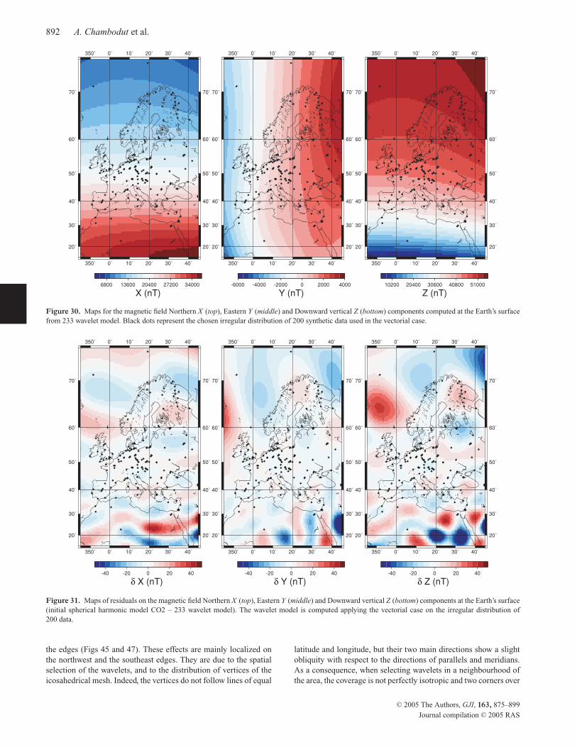
892 A. Chambodut et al.
350˚
350˚
0˚
0˚
10˚
10˚
20˚
20˚
30˚
30˚
40˚
40˚
20˚ 20˚
30˚ 30˚
40˚ 40˚
50˚ 50˚
60˚ 60˚
70˚ 70˚
6800 13600 20400 27200 34000
X (nT)
350˚
350˚
0˚
0˚
10˚
10˚
20˚
20˚
30˚
30˚
40˚
40˚
20˚ 20˚
30˚ 30˚
40˚ 40˚
50˚ 50˚
60˚ 60˚
70˚ 70˚
-6000 -4000 -2000 0 2000 4000
Y (nT)
350˚
350˚
0˚
0˚
10˚
10˚
20˚
20˚
30˚
30˚
40˚
40˚
20˚ 20˚
30˚ 30˚
40˚ 40˚
50˚ 50˚
60˚ 60˚
70˚ 70˚
10200 20400 30600 40800 51000
Z (nT)
Figure 30. Maps for the magnetic field Northern X (top), Eastern Y (middle) and Downward vertical Z (bottom) components computed at the Earth’s surface
from 233 wavelet model. Black dots represent the chosen irregular distribution of 200 synthetic data used in the vectorial case.
350˚
350˚
0˚
0˚
10˚
10˚
20˚
20˚
30˚
30˚
40˚
40˚
20˚ 20˚
30˚ 30˚
40˚ 40˚
50˚ 50˚
60˚ 60˚
70˚ 70˚
-40 -20 0 20 40
δ X (nT)
350˚
350˚
0˚
0˚
10˚
10˚
20˚
20˚
30˚
30˚
40˚
40˚
20˚ 20˚
30˚ 30˚
40˚ 40˚
50˚ 50˚
60˚ 60˚
70˚ 70˚
-40 -20 0 20 40
δ Y (nT)
350˚
350˚
0˚
0˚
10˚
10˚
20˚
20˚
30˚
30˚
40˚
40˚
20˚ 20˚
30˚ 30˚
40˚ 40˚
50˚ 50˚
60˚ 60˚
70˚ 70˚
-40 -20 0 20 40
δ Z (nT)
Figure 31. Maps of residuals on the magnetic field Northern X (top), Eastern Y (middle) and Downward vertical Z (bottom) components at the Earth’s surface
(initial spherical harmonic model CO2 – 233 wavelet model). The wavelet model is computed applying the vectorial case on the irregular distribution of
200 data.
the edges (Figs 45 and 47). These effects are mainly localized on
the northwest and the southeast edges. They are due to the spatial
selection of the wavelets, and to the distribution of vertices of the
icosahedrical mesh. Indeed, the vertices do not follow lines of equal
latitude and longitude, but their two main directions show a slight
obliquity with respect to the directions of parallels and meridians.
As a consequence, when selecting wavelets in a neighbourhood of
the area, the coverage is not perfectly isotropic and two corners over
C© 2005 The Authors, GJI, 163, 875–899
Journal compilation C© 2005 RAS
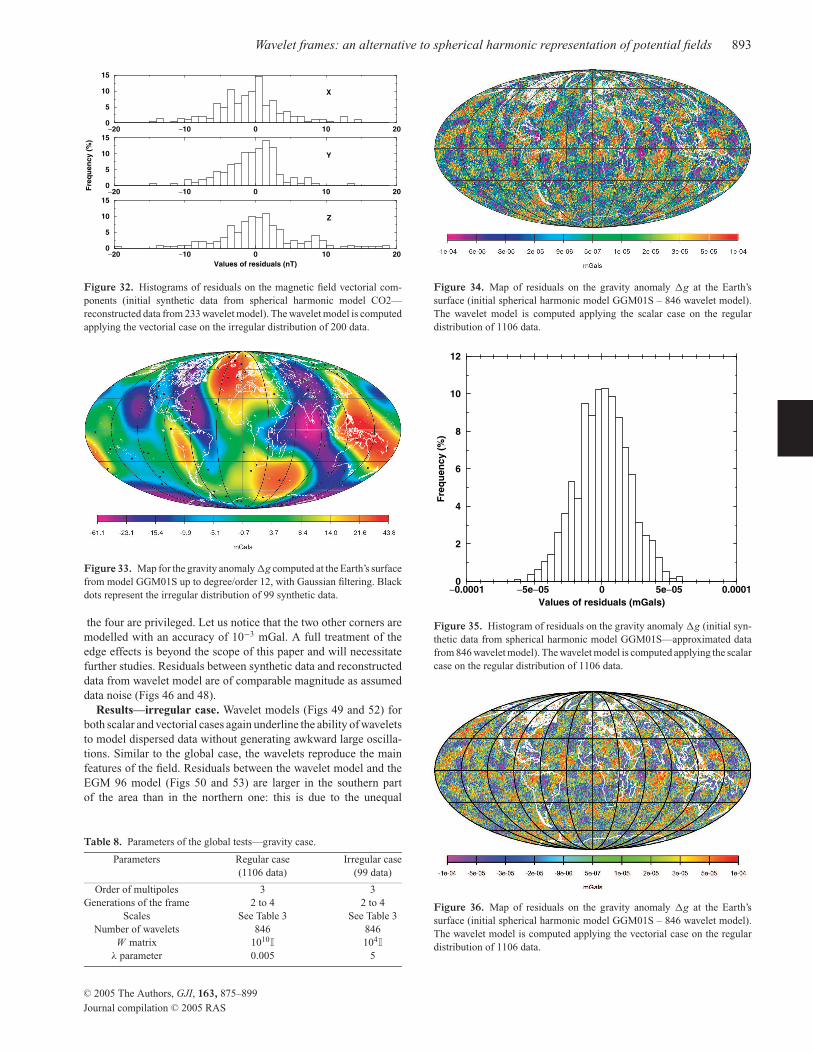
Wavelet frames: an alternative to spherical harmonic representation of potential fields 893
−20 −10 0 10 20
Values of residuals (nT)
0
5
10
15
Fre
qu
en
cy
(%
)
−20 −10 0 10 200
5
10
15−20 −10 0 10 20
0
5
10
15
X
Y
Z
Figure 32. Histograms of residuals on the magnetic field vectorial com-
ponents (initial synthetic data from spherical harmonic model CO2—
reconstructed data from 233 wavelet model). The wavelet model is computed
applying the vectorial case on the irregular distribution of 200 data.
Figure 33. Map for the gravity anomaly �g computed at the Earth’s surface
from model GGM01S up to degree/order 12, with Gaussian filtering. Black
dots represent the irregular distribution of 99 synthetic data.
the four are privileged. Let us notice that the two other corners are
modelled with an accuracy of 10−3 mGal. A full treatment of the
edge effects is beyond the scope of this paper and will necessitate
further studies. Residuals between synthetic data and reconstructed
data from wavelet model are of comparable magnitude as assumed
data noise (Figs 46 and 48).
Results—irregular case. Wavelet models (Figs 49 and 52) for
both scalar and vectorial cases again underline the ability of wavelets
to model dispersed data without generating awkward large oscilla-
tions. Similar to the global case, the wavelets reproduce the main
features of the field. Residuals between the wavelet model and the
EGM 96 model (Figs 50 and 53) are larger in the southern part
of the area than in the northern one: this is due to the unequal
Table 8. Parameters of the global tests—gravity case.
Parameters Regular case Irregular case
(1106 data) (99 data)
Order of multipoles 3 3
Generations of the frame 2 to 4 2 to 4
Scales See Table 3 See Table 3
Number of wavelets 846 846
W matrix 1010I 104
I
λ parameter 0.005 5
Figure 34. Map of residuals on the gravity anomaly �g at the Earth’s
surface (initial spherical harmonic model GGM01S – 846 wavelet model).
The wavelet model is computed applying the scalar case on the regular
distribution of 1106 data.
−0.0001 −5e−05 0 5e−05 0.0001
Values of residuals (mGals)
0
2
4
6
8
10
12
Fre
qu
en
cy
(%
)
Figure 35. Histogram of residuals on the gravity anomaly �g (initial syn-
thetic data from spherical harmonic model GGM01S—approximated data
from 846 wavelet model). The wavelet model is computed applying the scalar
case on the regular distribution of 1106 data.
Figure 36. Map of residuals on the gravity anomaly �g at the Earth’s
surface (initial spherical harmonic model GGM01S – 846 wavelet model).
The wavelet model is computed applying the vectorial case on the regular
distribution of 1106 data.
C© 2005 The Authors, GJI, 163, 875–899
Journal compilation C© 2005 RAS
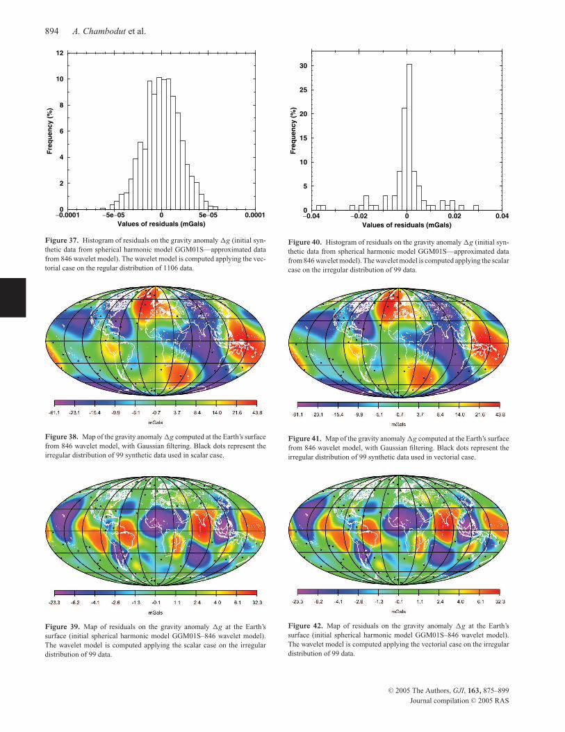
894 A. Chambodut et al.
−0.0001 −5e−05 0 5e−05 0.0001
Values of residuals (mGals)
0
2
4
6
8
10
12F
req
ue
nc
y (
%)
Figure 37. Histogram of residuals on the gravity anomaly �g (initial syn-
thetic data from spherical harmonic model GGM01S—approximated data
from 846 wavelet model). The wavelet model is computed applying the vec-
torial case on the regular distribution of 1106 data.
Figure 38. Map of the gravity anomaly �g computed at the Earth’s surface
from 846 wavelet model, with Gaussian filtering. Black dots represent the
irregular distribution of 99 synthetic data used in scalar case.
Figure 39. Map of residuals on the gravity anomaly �g at the Earth’s
surface (initial spherical harmonic model GGM01S–846 wavelet model).
The wavelet model is computed applying the scalar case on the irregular
distribution of 99 data.
−0.04 −0.02 0 0.02 0.04
Values of residuals (mGals)
0
5
10
15
20
25
30
Fre
qu
en
cy
(%
)
Figure 40. Histogram of residuals on the gravity anomaly �g (initial syn-
thetic data from spherical harmonic model GGM01S—approximated data
from 846 wavelet model). The wavelet model is computed applying the scalar
case on the irregular distribution of 99 data.
Figure 41. Map of the gravity anomaly �g computed at the Earth’s surface
from 846 wavelet model, with Gaussian filtering. Black dots represent the
irregular distribution of 99 synthetic data used in vectorial case.
Figure 42. Map of residuals on the gravity anomaly �g at the Earth’s
surface (initial spherical harmonic model GGM01S–846 wavelet model).
The wavelet model is computed applying the vectorial case on the irregular
distribution of 99 data.
C© 2005 The Authors, GJI, 163, 875–899
Journal compilation C© 2005 RAS
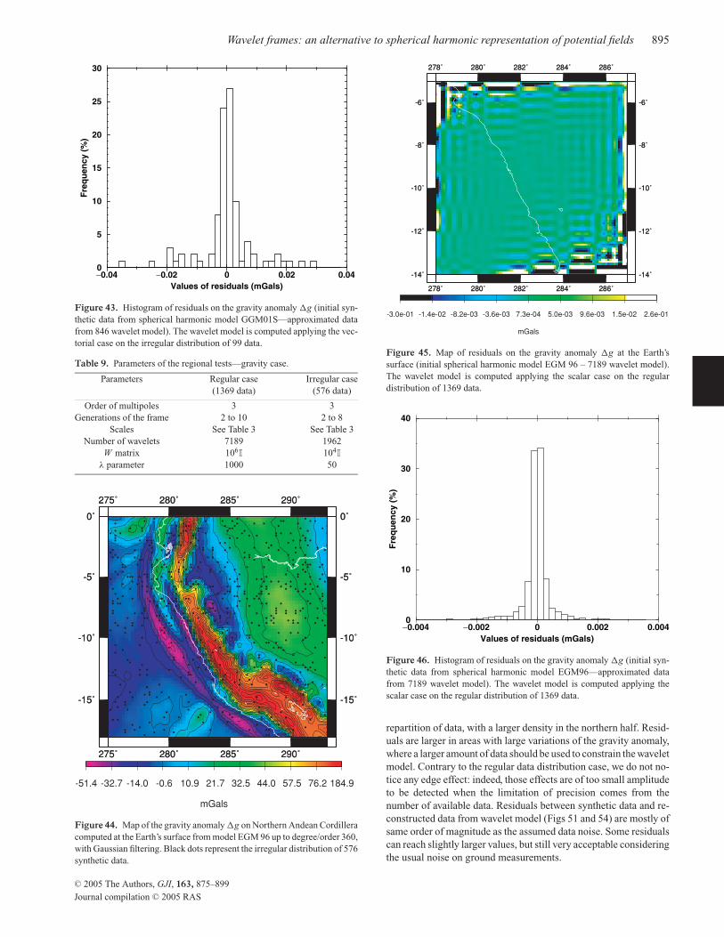
Wavelet frames: an alternative to spherical harmonic representation of potential fields 895
−0.04 −0.02 0 0.02 0.04
Values of residuals (mGals)
0
5
10
15
20
25
30
Fre
qu
en
cy
(%
)
Figure 43. Histogram of residuals on the gravity anomaly �g (initial syn-
thetic data from spherical harmonic model GGM01S—approximated data
from 846 wavelet model). The wavelet model is computed applying the vec-
torial case on the irregular distribution of 99 data.
Table 9. Parameters of the regional tests—gravity case.
Parameters Regular case Irregular case
(1369 data) (576 data)
Order of multipoles 3 3
Generations of the frame 2 to 10 2 to 8
Scales See Table 3 See Table 3
Number of wavelets 7189 1962
W matrix 106I 104
I
λ parameter 1000 50
275˚
275˚
280˚
280˚
285˚
285˚
290˚
290˚
-15˚ -15˚
-10˚ -10˚
-5˚ -5˚
0˚ 0˚
275˚
275˚
280˚
280˚
285˚
285˚
290˚
290˚
-15˚ -15˚
-10˚ -10˚
-5˚ -5˚
0˚ 0˚
-51.4 -32.7 -14.0 -0.6 10.9 21.7 32.5 44.0 57.5 76.2 184.9
mGals
Figure 44. Map of the gravity anomaly �g on Northern Andean Cordillera
computed at the Earth’s surface from model EGM 96 up to degree/order 360,
with Gaussian filtering. Black dots represent the irregular distribution of 576
synthetic data.
278˚
278˚
280˚
280˚
282˚
282˚
284˚
284˚
286˚
286˚
-14˚ -14˚
-12˚ -12˚
-10˚ -10˚
-8˚ -8˚
-6˚ -6˚
278˚
278˚
280˚
280˚
282˚
282˚
284˚
284˚
286˚
286˚
-14˚ -14˚
-12˚ -12˚
-10˚ -10˚
-8˚ -8˚
-6˚ -6˚
-3.0e-01 -1.4e-02 -8.2e-03 -3.6e-03 7.3e-04 5.0e-03 9.6e-03 1.5e-02 2.6e-01
mGals
Figure 45. Map of residuals on the gravity anomaly �g at the Earth’s
surface (initial spherical harmonic model EGM 96 – 7189 wavelet model).
The wavelet model is computed applying the scalar case on the regular
distribution of 1369 data.
−0.004 −0.002 0 0.002 0.004
Values of residuals (mGals)
0
10
20
30
40
Fre
qu
en
cy
(%
)
Figure 46. Histogram of residuals on the gravity anomaly �g (initial syn-
thetic data from spherical harmonic model EGM96—approximated data
from 7189 wavelet model). The wavelet model is computed applying the
scalar case on the regular distribution of 1369 data.
repartition of data, with a larger density in the northern half. Resid-
uals are larger in areas with large variations of the gravity anomaly,
where a larger amount of data should be used to constrain the wavelet
model. Contrary to the regular data distribution case, we do not no-
tice any edge effect: indeed, those effects are of too small amplitude
to be detected when the limitation of precision comes from the
number of available data. Residuals between synthetic data and re-
constructed data from wavelet model (Figs 51 and 54) are mostly of
same order of magnitude as the assumed data noise. Some residuals
can reach slightly larger values, but still very acceptable considering
the usual noise on ground measurements.
C© 2005 The Authors, GJI, 163, 875–899
Journal compilation C© 2005 RAS
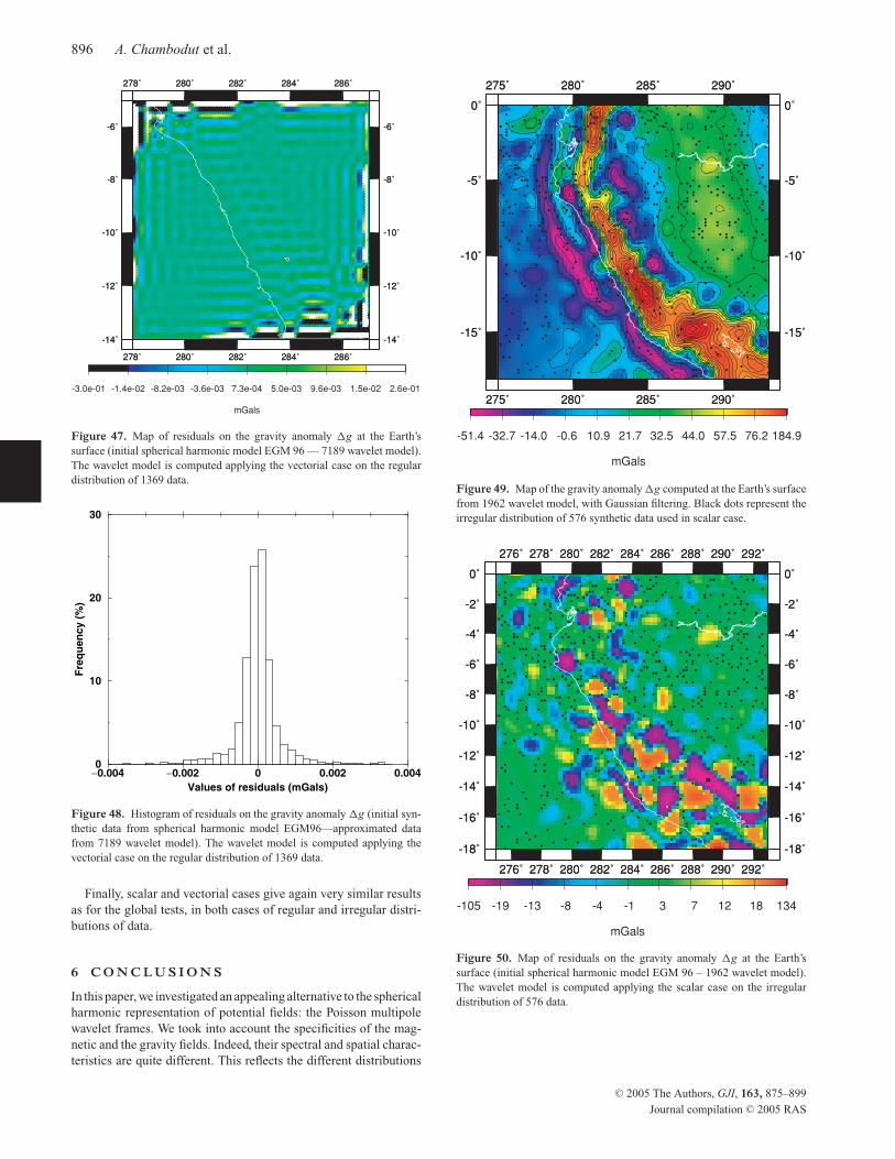
896 A. Chambodut et al.
278˚
278˚
280˚
280˚
282˚
282˚
284˚
284˚
286˚
286˚
-14˚ -14˚
-12˚ -12˚
-10˚ -10˚
-8˚ -8˚
-6˚ -6˚
278˚
278˚
280˚
280˚
282˚
282˚
284˚
284˚
286˚
286˚
-14˚ -14˚
-12˚ -12˚
-10˚ -10˚
-8˚ -8˚
-6˚ -6˚
-3.0e-01 -1.4e-02 -8.2e-03 -3.6e-03 7.3e-04 5.0e-03 9.6e-03 1.5e-02 2.6e-01
mGals
Figure 47. Map of residuals on the gravity anomaly �g at the Earth’s
surface (initial spherical harmonic model EGM 96 — 7189 wavelet model).
The wavelet model is computed applying the vectorial case on the regular
distribution of 1369 data.
−0.004 −0.002 0 0.002 0.004
Values of residuals (mGals)
0
10
20
30
Fre
qu
en
cy
(%
)
Figure 48. Histogram of residuals on the gravity anomaly �g (initial syn-
thetic data from spherical harmonic model EGM96—approximated data
from 7189 wavelet model). The wavelet model is computed applying the
vectorial case on the regular distribution of 1369 data.
Finally, scalar and vectorial cases give again very similar results
as for the global tests, in both cases of regular and irregular distri-
butions of data.
6 C O N C L U S I O N S
In this paper, we investigated an appealing alternative to the spherical
harmonic representation of potential fields: the Poisson multipole
wavelet frames. We took into account the specificities of the mag-
netic and the gravity fields. Indeed, their spectral and spatial charac-
teristics are quite different. This reflects the different distributions
275˚
275˚
280˚
280˚
285˚
285˚
290˚
290˚
-15˚ -15˚
-10˚ -10˚
-5˚ -5˚
0˚ 0˚
275˚
275˚
280˚
280˚
285˚
285˚
290˚
290˚
-15˚ -15˚
-10˚ -10˚
-5˚ -5˚
0˚ 0˚
-51.4 -32.7 -14.0 -0.6 10.9 21.7 32.5 44.0 57.5 76.2 184.9
mGals
Figure 49. Map of the gravity anomaly �g computed at the Earth’s surface
from 1962 wavelet model, with Gaussian filtering. Black dots represent the
irregular distribution of 576 synthetic data used in scalar case.
276˚
276˚
278˚
278˚
280˚
280˚
282˚
282˚
284˚
284˚
286˚
286˚
288˚
288˚
290˚
290˚
292˚
292˚
-18˚ -18˚
-16˚ -16˚
-14˚ -14˚
-12˚ -12˚
-10˚ -10˚
-8˚ -8˚
-6˚ -6˚
-4˚ -4˚
-2˚ -2˚
0˚ 0˚
276˚
276˚
278˚
278˚
280˚
280˚
282˚
282˚
284˚
284˚
286˚
286˚
288˚
288˚
290˚
290˚
292˚
292˚
-18˚ -18˚
-16˚ -16˚
-14˚ -14˚
-12˚ -12˚
-10˚ -10˚
-8˚ -8˚
-6˚ -6˚
-4˚ -4˚
-2˚ -2˚
0˚ 0˚
-105 -19 -13 -8 -4 -1 3 7 12 18 134
mGals
Figure 50. Map of residuals on the gravity anomaly �g at the Earth’s
surface (initial spherical harmonic model EGM 96 – 1962 wavelet model).
The wavelet model is computed applying the scalar case on the irregular
distribution of 576 data.
C© 2005 The Authors, GJI, 163, 875–899
Journal compilation C© 2005 RAS
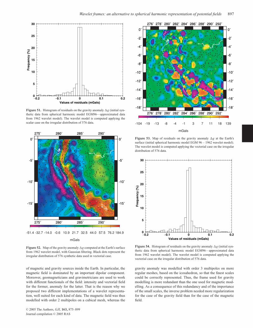
Wavelet frames: an alternative to spherical harmonic representation of potential fields 897
−0.2 −0.1 0 0.1 0.2
Values of residuals (mGals)
0
5
10
15
20
25
30
Fre
qu
en
cy
(%
)
Figure 51. Histogram of residuals on the gravity anomaly �g (initial syn-
thetic data from spherical harmonic model EGM96—approximated data
from 1962 wavelet model). The wavelet model is computed applying the
scalar case on the irregular distribution of 576 data.
275˚
275˚
280˚
280˚
285˚
285˚
290˚
290˚
-15˚ -15˚
-10˚ -10˚
-5˚ -5˚
0˚ 0˚
275˚
275˚
280˚
280˚
285˚
285˚
290˚
290˚
-15˚ -15˚
-10˚ -10˚
-5˚ -5˚
0˚ 0˚
-51.4 -32.7 -14.0 -0.6 10.9 21.7 32.5 44.0 57.5 76.2 184.9
mGals
Figure 52. Map of the gravity anomaly �g computed at the Earth’s surface
from 1962 wavelet model, with Gaussian filtering. Black dots represent the
irregular distribution of 576 synthetic data used in vectorial case.
of magnetic and gravity sources inside the Earth. In particular, the
magnetic field is dominated by an important dipolar component.
Moreover, geomagneticians and gravimetricians are used to work
with different functionals of the field: intensity and vectorial field
for the former, anomaly for the latter. That is the reason why we
proposed two different implementations of a wavelet representa-
tion, well suited for each kind of data. The magnetic field was thus
modelled with order 2 multipoles on a cubical mesh, whereas the
276˚
276˚
278˚
278˚
280˚
280˚
282˚
282˚
284˚
284˚
286˚
286˚
288˚
288˚
290˚
290˚
292˚
292˚
-18˚ -18˚
-16˚ -16˚
-14˚ -14˚
-12˚ -12˚
-10˚ -10˚
-8˚ -8˚
-6˚ -6˚
-4˚ -4˚
-2˚ -2˚
0˚ 0˚
276˚
276˚
278˚
278˚
280˚
280˚
282˚
282˚
284˚
284˚
286˚
286˚
288˚
288˚
290˚
290˚
292˚
292˚
-18˚ -18˚
-16˚ -16˚
-14˚ -14˚
-12˚ -12˚
-10˚ -10˚
-8˚ -8˚
-6˚ -6˚
-4˚ -4˚
-2˚ -2˚
0˚ 0˚
-104 -19 -13 -8 -4 -1 3 7 11 18 139
mGals
Figure 53. Map of residuals on the gravity anomaly �g at the Earth’s
surface (initial spherical harmonic model EGM 96 – 1962 wavelet model).
The wavelet model is computed applying the vectorial case on the irregular
distribution of 576 data.
−0.2 −0.1 0 0.1 0.2
Values of residuals (mGals)
0
5
10
15
20
25
30
Fre
qu
en
cy
(%
)
Figure 54. Histogram of residuals on the gravity anomaly �g (initial syn-
thetic data from spherical harmonic model EGM96—approximated data
from 1962 wavelet model). The wavelet model is computed applying the
vectorial case on the irregular distribution of 576 data.
gravity anomaly was modelled with order 3 multipoles on more
regular meshes, based on the icosahedron, so that the finest scales
could be correctly represented. Thus, the frame used for gravity
modelling is more redundant than the one used for magnetic mod-
elling. As a consequence of this redundancy and of the importance
of the small scales, the inverse problem needed more regularization
for the case of the gravity field than for the case of the magnetic
field.
C© 2005 The Authors, GJI, 163, 875–899
Journal compilation C© 2005 RAS
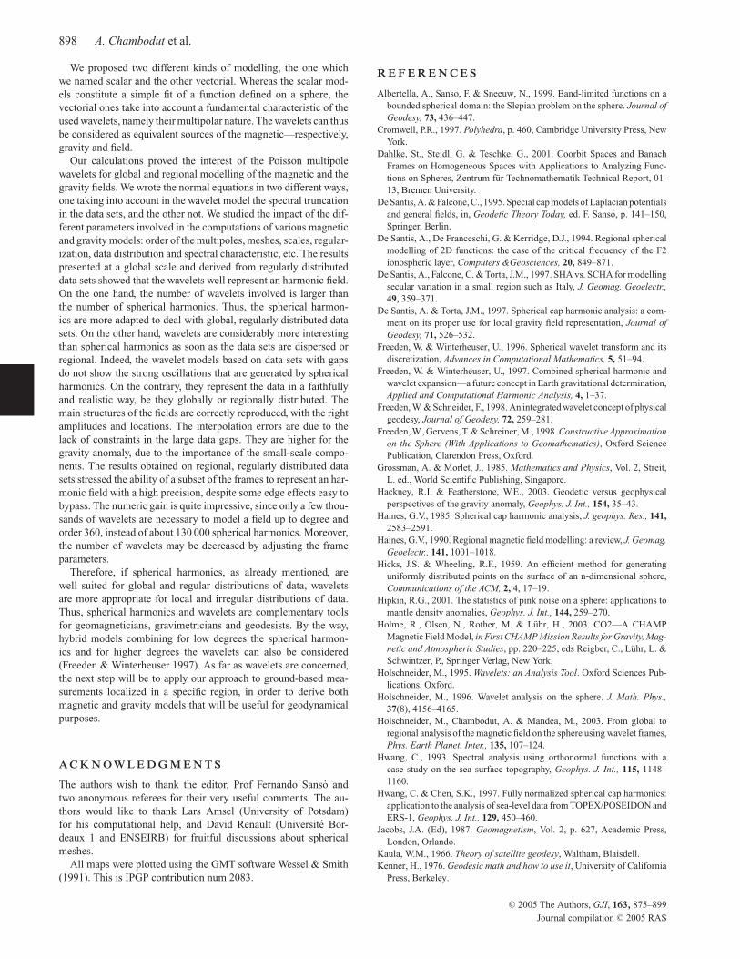
898 A. Chambodut et al.
We proposed two different kinds of modelling, the one which
we named scalar and the other vectorial. Whereas the scalar mod-
els constitute a simple fit of a function defined on a sphere, the
vectorial ones take into account a fundamental characteristic of the
used wavelets, namely their multipolar nature. The wavelets can thus
be considered as equivalent sources of the magnetic—respectively,
gravity and field.
Our calculations proved the interest of the Poisson multipole
wavelets for global and regional modelling of the magnetic and the
gravity fields. We wrote the normal equations in two different ways,
one taking into account in the wavelet model the spectral truncation
in the data sets, and the other not. We studied the impact of the dif-
ferent parameters involved in the computations of various magnetic
and gravity models: order of the multipoles, meshes, scales, regular-
ization, data distribution and spectral characteristic, etc. The results
presented at a global scale and derived from regularly distributed
data sets showed that the wavelets well represent an harmonic field.
On the one hand, the number of wavelets involved is larger than
the number of spherical harmonics. Thus, the spherical harmon-
ics are more adapted to deal with global, regularly distributed data
sets. On the other hand, wavelets are considerably more interesting
than spherical harmonics as soon as the data sets are dispersed or
regional. Indeed, the wavelet models based on data sets with gaps
do not show the strong oscillations that are generated by spherical
harmonics. On the contrary, they represent the data in a faithfully
and realistic way, be they globally or regionally distributed. The
main structures of the fields are correctly reproduced, with the right
amplitudes and locations. The interpolation errors are due to the
lack of constraints in the large data gaps. They are higher for the
gravity anomaly, due to the importance of the small-scale compo-
nents. The results obtained on regional, regularly distributed data
sets stressed the ability of a subset of the frames to represent an har-
monic field with a high precision, despite some edge effects easy to
bypass. The numeric gain is quite impressive, since only a few thou-
sands of wavelets are necessary to model a field up to degree and
order 360, instead of about 130 000 spherical harmonics. Moreover,
the number of wavelets may be decreased by adjusting the frame
parameters.
Therefore, if spherical harmonics, as already mentioned, are
well suited for global and regular distributions of data, wavelets
are more appropriate for local and irregular distributions of data.
Thus, spherical harmonics and wavelets are complementary tools
for geomagneticians, gravimetricians and geodesists. By the way,
hybrid models combining for low degrees the spherical harmon-
ics and for higher degrees the wavelets can also be considered
(Freeden & Winterheuser 1997). As far as wavelets are concerned,
the next step will be to apply our approach to ground-based mea-
surements localized in a specific region, in order to derive both
magnetic and gravity models that will be useful for geodynamical
purposes.
A C K N O W L E D G M E N T S
The authors wish to thank the editor, Prof Fernando Sanso and
two anonymous referees for their very useful comments. The au-
thors would like to thank Lars Amsel (University of Potsdam)
for his computational help, and David Renault (Universite Bor-
deaux 1 and ENSEIRB) for fruitful discussions about spherical
meshes.
All maps were plotted using the GMT software Wessel & Smith
(1991). This is IPGP contribution num 2083.
R E F E R E N C E S
Albertella, A., Sanso, F. & Sneeuw, N., 1999. Band-limited functions on a
bounded spherical domain: the Slepian problem on the sphere. Journal of
Geodesy, 73, 436–447.
Cromwell, P.R., 1997. Polyhedra, p. 460, Cambridge University Press, New
York.
Dahlke, St., Steidl, G. & Teschke, G., 2001. Coorbit Spaces and Banach
Frames on Homogeneous Spaces with Applications to Analyzing Func-
tions on Spheres, Zentrum fur Technomathematik Technical Report, 01-
13, Bremen University.
De Santis, A. & Falcone, C., 1995. Special cap models of Laplacian potentials
and general fields, in, Geodetic Theory Today, ed. F. Sanso, p. 141–150,
Springer, Berlin.
De Santis, A., De Franceschi, G. & Kerridge, D.J., 1994. Regional spherical
modelling of 2D functions: the case of the critical frequency of the F2
ionospheric layer, Computers &Geosciences, 20, 849–871.
De Santis, A., Falcone, C. & Torta, J.M., 1997. SHA vs. SCHA for modelling
secular variation in a small region such as Italy, J. Geomag. Geoelectr.,
49, 359–371.
De Santis, A. & Torta, J.M., 1997. Spherical cap harmonic analysis: a com-
ment on its proper use for local gravity field representation, Journal of
Geodesy, 71, 526–532.
Freeden, W. & Winterheuser, U., 1996. Spherical wavelet transform and its
discretization, Advances in Computational Mathematics, 5, 51–94.
Freeden, W. & Winterheuser, U., 1997. Combined spherical harmonic and
wavelet expansion—a future concept in Earth gravitational determination,
Applied and Computational Harmonic Analysis, 4, 1–37.
Freeden, W. & Schneider, F., 1998. An integrated wavelet concept of physical
geodesy, Journal of Geodesy, 72, 259–281.
Freeden, W., Gervens, T. & Schreiner, M., 1998. Constructive Approximation
on the Sphere (With Applications to Geomathematics), Oxford Science
Publication, Clarendon Press, Oxford.
Grossman, A. & Morlet, J., 1985. Mathematics and Physics, Vol. 2, Streit,
L. ed., World Scientific Publishing, Singapore.
Hackney, R.I. & Featherstone, W.E., 2003. Geodetic versus geophysical
perspectives of the gravity anomaly, Geophys. J. Int., 154, 35–43.
Haines, G.V., 1985. Spherical cap harmonic analysis, J. geophys. Res., 141,
2583–2591.
Haines, G.V., 1990. Regional magnetic field modelling: a review, J. Geomag.
Geoelectr., 141, 1001–1018.
Hicks, J.S. & Wheeling, R.F., 1959. An efficient method for generating
uniformly distributed points on the surface of an n-dimensional sphere,
Communications of the ACM, 2, 4, 17–19.
Hipkin, R.G., 2001. The statistics of pink noise on a sphere: applications to
mantle density anomalies, Geophys. J. Int., 144, 259–270.
Holme, R., Olsen, N., Rother, M. & Luhr, H., 2003. CO2—A CHAMP
Magnetic Field Model, in First CHAMP Mission Results for Gravity, Mag-
netic and Atmospheric Studies, pp. 220–225, eds Reigber, C., Luhr, L. &
Schwintzer, P., Springer Verlag, New York.
Holschneider, M., 1995. Wavelets: an Analysis Tool. Oxford Sciences Pub-
lications, Oxford.
Holschneider, M., 1996. Wavelet analysis on the sphere. J. Math. Phys.,
37(8), 4156–4165.
Holschneider, M., Chambodut, A. & Mandea, M., 2003. From global to
regional analysis of the magnetic field on the sphere using wavelet frames,
Phys. Earth Planet. Inter., 135, 107–124.
Hwang, C., 1993. Spectral analysis using orthonormal functions with a
case study on the sea surface topography, Geophys. J. Int., 115, 1148–
1160.
Hwang, C. & Chen, S.K., 1997. Fully normalized spherical cap harmonics:
application to the analysis of sea-level data from TOPEX/POSEIDON and
ERS-1, Geophys. J. Int., 129, 450–460.
Jacobs, J.A. (Ed), 1987. Geomagnetism, Vol. 2, p. 627, Academic Press,
London, Orlando.
Kaula, W.M., 1966. Theory of satellite geodesy, Waltham, Blaisdell.
Kenner, H., 1976. Geodesic math and how to use it, University of California
Press, Berkeley.
C© 2005 The Authors, GJI, 163, 875–899
Journal compilation C© 2005 RAS

Wavelet frames: an alternative to spherical harmonic representation of potential fields 899
Korte, M. & Haak, V., 2000. Modelling European Magnetic Repeat Station
Data by SCHA in search of time-varying anomalies, Phys. Earth Planet.
Inter., 122, 205–220.
Lemoine, F.G. et al., 1998. The development of the joint NASA GSFC and
the National Imagery and Mapping Agency (NIMA) geopotential model
EGM96. NASA/TP – 1998 – 206861, Greenbelt, Maryland.
Li, J., Chao, D. & Ning, J., 1995. Spherical cap harmonic expansion for local
gravity field representation. Manuscripta Geodaetica, 20, 265–277.
Lowes, F.J., 1974. Spatial power spectrum of the main geomagnetic field and
estrapolation to the core, Geophys. J. R. astr. Soc., 36, 717–730.
Martelet, G., Sailhac, P., Moreau, F. & Diament, M., 2001. Characterization
of geological boundaries using 1D-wavelet transform on gravity data:
Theory and application to the Himalaya, Geophysics, 66(4), 1116–1129.
Mauersberger, P., 1956. Das Mittel der Energiedichte des geomagnetischen
Hauptfeldes an der Erdoberflache und seine sakulare Aenderung. Ger-
lands Beitr. Geophys., 65, 207–215.
Merrill, R.T., McElhinny, M.W. & McFadden, P.L., 1996. The Magnetic
Field of the Earth, Academic Press, San Diego.
Moritz, H., 1989. Advanced Physical Geodesy, 2nd edn, Wichmann,
Karlsruhe.
Muller, M.E., 1959. A note on a method for generating points uniformly on
N-dimensional spheres, Comm. Assoc. Comput. Mach., 2, 19–20.
Rummel, R. & van Gelderen, M., 1995. Meissl scheme—spectral character-
istics of physical geodesy. Manuscripta Geodaetica, 20, 379–385.
Sailhac, P., Galdeano, A., Gibert, D., Moreau, F. & Delor, C., 2000. Identi-
fication of sources of potential fields with the continuous wavelet trans-
form: complex wavelets and application to aeromagnetic profiles in French
Guiana. J. geophys. Res., 105, B8, 19 455–19 475.
Sailhac, P. & Gibert, D., 2003. Identification of sources of poten-
tial fields with the continuous wavelet transform: Two-dimensional
wavelets and multipolar approximations. J. geophys. Res., 108, B5, 2262,
doi:10.1029/2002JB002021.
Sandwell, D.T. & Renkin, M.L., 1988. Compensation of swells and plateaus
in the North Pacific: no direct evidence for mantle convection. J. geophys.
Res., 93, 2775–2783.
Schroeder, P. & Sweldens, W., 1995. Spherical wavelets: efficiently repre-
senting functions on the sphere. Computer Graphics Proceedings (SIG-
GRAPH 95), 161–172.
Tapley, B.D., Bettadpur, S., Watkins, M. & Reigber, C., 2004. The grav-
ity recovery and climate experiment: mission overview and early results.
Geophys. Res. Lett., 31, L09607:10.1029/2004GL019920.
Tarantola, A., 1987. Inverse problem theory, Elsevier, New York.
Thebault, E., Schott, J.J., Mandea, M. & Hoffbeck, J.P., 2004. A new proposal
for spherical cap harmonic analysis. Geophys. J. Int., 159, 83–103.
Wessel, P. & Smith, W.H.F., 1991. Free software helps map and display data.
Eos Trans. Am. geophys. Un., 729, 441.
C© 2005 The Authors, GJI, 163, 875–899
Journal compilation C© 2005 RAS