Wealth Taxation and Household Saving

Wealth Taxation and Household Saving:Evidence from Assessment Discontinuities in Norway

Marius A. K. Ring∗

November 7, 2021

Abstract

While it is common to assume that wealth taxation has a negative effect on householdsaving, neither theory nor existing empirical evidence lends clear support. Theoretically,the effect is ambiguous due to opposing income and substitution effects, and empirically,the effect is challenging to discern because of (mis)reporting responses. Using geographicdiscontinuities in the Norwegian annual net-wealth tax and third-party reported data onsavings, I find that wealth taxation causes households to save more, and that this increase insaving is primarily financed by increased labor earnings. These responses are the combinationof small negative effects of increasing the marginal tax rates on wealth and relatively largerpositive effects of increasing average rates. These findings imply that income effects maydominate substitution effects in household responses to rate-of-return shocks, which hasimportant implications for both optimal taxation and macroeconomic modeling.

Keywords: Wealth Taxes, Savings, Capital Taxation, Intertemporal SubstitutionJEL: G51, D14, D15, H20, H31, E21, J22

∗University of Texas at Austin and Statistics Norway. E-mail: [email protected]. I thankmy advisors, Dimitris Papanikolaou, Anthony DeFusco, and Matthew Notowidigdo for helpful comments andadvice. I owe considerable gratitude to Andreas Fagereng and Thor O. Thoresen for their help in initiatingthis research project, as well as their continued support. I thank Scott Baker, Kjetil Storesletten, Liam Brunt,Jim Poterba, Espen Henriksen, Henrik Kleven, Martin B. Holm, Matthias Doepke, Krisztina Molnar, ManudeepBhuller, Evelina Gavrilova, Enrichetta Ravina, SeHyoun Ahn, Gernot Doppelhofer, Jacopo Ponticelli, VictoriaMarone, Tore Ring, Floris Zoutman, Annette Vissing-Jørgensen, and Alina Bartscher for helpful comments anddiscussions, and participants at the Kellogg Finance bag-lunch seminars, Statistics Norway, Skatteforum, NHHNorwegian School of Economics, London Business School, BI Norwegian Business School, Drexel, Yale, NYU, UTDallas, WUSTL, Stanford, UCLA, MIT, Wisconsin-Madison, UT Austin, the Center for Retirement Research atBoston College, the Nordic Junior Macro Seminar, the NBER Summer Institute Public Economics workshop, theUniversity of Oslo, and Einaudi (EIEF) for helpful comments and questions. Support from the Research Councilof Norway (grant #283315) is gratefully acknowledged.

1 Introduction

How households respond to changes in the net-of-tax rate of return is crucial to both optimalcapital taxation and macroeconomic modeling. In optimal capital taxation, it determines theextent of distortionary effects on saving behavior and labor supply. Quantifying these distor-tions is necessary for determining the optimal tax policy (Atkinson and Sandmo 1980, Strauband Werning 2020, Saez and Stantcheva 2018). In macroeconomics, it determines the ability ofstandard representative agent models to explain the aggregate effects of monetary policy (Ka-plan, Moll, and Violante, 2018) and informs the importance of different transmission channels(Auclert 2019, Wong 2019, Caramp and Silva 2020). It is also informative of whether savingresponses dampen or amplify downward movements in the natural interest rate (Mian, Straub,and Sufi 2021, Summers and Rachel 2019). More generally, empirical responses to rate-of-returnshocks inform the Elasticity of Intertemporal Substitution (EIS). The EIS is a key parameterin virtually all economic models that involve intertemporal decision-making, but there is noconsensus on what it should be.

Despite this broad importance, there is a dearth of applicable empirical evidence. Identifyingvariation in the after-tax rate of return is scarce. Even exogenous shocks to the interest rate mayhave general equilibrium effects that inhibit the identification of the pure rate-of-return effectneeded to inform micro-founded models. A potential solution is to exploit variation in capitaltaxation caused by peculiarities in the tax code to identify partial-equilibrium effects. However,this strategy typically presents important problems related to both identification and measure-ment. First, one must often compare households who differ on tax-relevant characteristics, suchas wealth or gross income, that are also determinants of saving behavior. Second, even if capitaltaxation were randomly assigned, data limitations may preclude researchers from distinguishingbetween real saving responses and tax evasion. This is problematic, since evasion responses areuninformative of responses to other rate-of-return shocks, such as interest rate changes, or evencapital taxation when evasion opportunities are limited.

These empirical challenges are complemented by a long-standing theoretical ambiguity abouteven the sign of saving responses to rate-of-return shocks.1 This ambiguity is due to counteringincome and substitution effects from increasing both the absolute and relative price of futureconsumption. Which effect dominates depends crucially on the EIS, for which the existing rangeof empirical estimates spans 0 to 2.2 This is an “enormous range in terms of its implicationsfor intertemporal behavior and policy” (Best, Cloyne, Ilzetzki, and Kleven, 2020) and includesstrikingly different household responses to economic news (Schmidt and Toda, 2019).

In this paper, I use a quasi-experimental setting in Norway that allows me to address theidentification and measurement challenges described above. The source of identifying variation1Boskin (1978) indirectly refers to the theoretical ambiguity in his seminal empirical paper: “In brief summary,there is very little empirical evidence upon which to infer a positive relationship (substitution effect outweighingincome effect) between saving and the real net rate-of-return to capital. Surprisingly little attention has beenpaid to this issue—particularly in light of its key role in answering many important policy questions—and thosestudies which do attempt to deal with it can be improved substantially.”

2In a standard life-cycle model without (non-capital) incomes, the income effect dominates whenever the EIS <1. Including (endogenous) labor income lowers this cutoff to around 0.45 in my setting (Section 5).

1

in the net-of-tax rate of return comes from capital taxation in the form of an annual net-wealthtax. While wealth taxation and capital income taxation are equivalent in standard models,3

wealth taxation differs from traditional capital income taxation by requiring regular assessmentsof the stock of capital. The steps the Norwegian government has taken to make such assessmentsprovides promising quasi-experimental variation in the net-of-tax rate of return.

In Norway, wealth taxes are levied annually as a 1 percent tax on taxable wealth that exceedsa given threshold. The relatively low threshold subjects 12 to 15 percent of taxpayers to thewealth tax, and primarily affects households in the top 10% of the life-time income distribution(Halvorsen and Thoresen, 2021). The main components of the tax base are financial wealth andhousing wealth. While financial wealth may be assessed at third-party reported market values(which limits the scope for evasion through misreporting), housing wealth must be determinedby the tax authorities. In 2010, the tax authorities implemented a new model to assess thehousing wealth component. This hedonic pricing model contained municipal fixed effects, whichimposed geographic discontinuities in assessed housing wealth even in the absence of any truediscontinuities in house prices. These discontinuities provide substantial identifying variationin taxable wealth, and thereby (i) whether households pay a wealth tax and (ii) the amountof wealth taxes they pay. This provides variation in both the marginal and average net-of-tax rate of return. I use data on structure-level ownership and location as well as the exactparameters of the hedonic pricing model to implement this novel identifying variation in aBoundary Discontinuity Design (BDD) approach.

I first consider the effect on yearly financial saving. My estimates imply that for each addi-tional NOK pushed above the tax threshold, and thereby subject to the wealth tax, householdsincrease their yearly financial saving by 0.038. These estimates adjust for the mechanical wealth-reducing effects of increased taxation and constitute evidence of behavioral responses to capitaltaxation that go in the opposite direction of what is typically assumed.4 This adjusted savingpropensity is almost three times larger than what is necessary to maintain the same level ofwealth after taxes are collected, consistent with households increasing their savings to offsetfuture wealth tax payments.

My findings indicate that this increase in saving is primarily financed by increases in laborsupply. Corresponding to the geographic discontinuities in wealth tax exposure, I find cleardiscontinuities in household labor earnings. These discontinuities constitute novel evidence of ameaningful cross-elasticity between labor supply and the net-of-tax return on capital. Translat-ing these estimates into an earnings propensity, I find that households increase their after-taxearnings by around 0.027 for each additional NOK subjected to the wealth tax, enough to financea majority of the additional saving.

I also present new evidence on the effect of capital taxation on portfolio allocation. I firstconsider the effect on the share of financial wealth invested in the stock market. The perhapsdominant hypothesis is that risk-averse agents will respond to a wealth-tax-induced drop in life3This includes Chamley (1986) and Judd (1985). For further discussion, see, e.g., Bastani and Waldenstrom(2018), Scheuer and Slemrod (2021), Guvenen, Kambourov, Kuruscu, Ocampo, and Chen (2019), and Lu (2021)

4References in the popular press to the potential disincentive effects of wealth or capital taxation are abundant. Ineconomic modeling, the typical assumption is that capital taxation reduces saving (Saez and Stantcheva, 2018)

2

time consumption by allocating less of their wealth to risky assets. The alternative view is thathouseholds respond to a drop in the after-tax return by “reaching for yield” or capital incomes,which may entail substituting low-interest deposits for higher-return stock holdings (see, e.g.,Lian, Ma, and Wang 2019; Daniel, Garlappi, and Xiao 2021; Campbell and Sigalov 2021).Consistent with this ambiguity, I find no effect on the risky share and can rule out economicallylarge effects. I further present the hypothesis that the adverse income effect of increased taxationmay induce households to enjoy less financial leisure, in the sense that they exert greater efforttoward financially optimizing the returns they receive on their low-risk savings. My findings,however, lend meager support to this hypothesis. For the average household, there is little effecton realized interest rates on deposits, which is the dominant form of risk-free saving.

I proceed by using a simple life-cycle model to illustrate which values of the EIS can rational-ize my empirical findings. This exercise shows how both the saving and labor earnings responsesare determined by the EIS. Depending on how preferences for leisure are parameterized, mypoint estimates are consistent with an EIS between 0.02 and 0.15. When the EIS exceeds 0.5,the life-cycle model produces positive saving and labor supply responses that are outside of the95% confidence intervals of my empirical findings.

The theoretical implication of my main findings on saving and labor supply responses is thatincome effects dominate intertemporal substitution effects. The positive income effects associ-ated with increasing the average tax rate on wealth (ATR) must be larger in magnitude than thenegative substitution effects caused by increasing the marginal tax rate (MTR). However, re-cent research shows that consumers may suboptimally confuse marginal and average prices (Ito,2014). If this applies to taxes as well, then traditional approaches to modeling non-linear, pro-gressive taxation would be fundamentally misguided. In light of this, I test whether householdsrespond to marginal and average tax rates as theory would prescribe. I use an instrumental-variables framework that exploits the fact that assessment discontinuities had differential effectson ATRs and MTRs depending on households’ ex-ante characteristics, such as initial taxablewealth. My findings are consistent with the underlying mechanism of the life-cycle model: Iestimate positive ATR effects that dominate weaker, negative MTR effects.

This paper contributes to multiple literatures. First, I contribute to the new literatureproviding a rich picture of behavioral responses to capital taxation (see, e.g., Boissel and Matray2021; Nekoei and Seim 2018; Arefeva, Davis, Ghent, and Park 2021; Glogowsky 2021; Lavecchiaand Tazhitdinova 2021; Martınez-Toledano 2020; Bjørneby, Markussen, and Røed 2020; Bach,Bozio, Guillouzouic, and Malgouyres 2020a; Tsoutsoura 2015). Starting with Seim (2017), acentral finding is that wealth taxation reduces the amount of taxable wealth that householdsreport (Seim 2017; Zoutman 2018; Brulhart, Gruber, Krapf, and Schmidheiny 2019; Londono-Velez and Avila-Mahecha 2020a; Londono-Velez and Avila-Mahecha 2020b; Jakobsen, Jakobsen,Kleven, and Zucman 2020; Duran-Cabre, Esteller-More, and Mas-Montserrat 2019). However,these findings do not necessarily imply that wealth taxes cause households to save less, asevasion responses may dominate (real) saving responses.5 Consistent with this ambiguity, I5Seim (2017) notes that evasion and avoidance responses contaminate the link between behavioral responses andthe structural parameters that govern real responses (i.e., the elasticity of intertemporal substitution). Usinga bunching design, Seim (2017) documents behavioral responses that are fully attributable to misreporting. A

3

find strikingly different effects when limiting the role for evasion by (i) focusing on savings inthe form of financial wealth, which in Norway is primarily third-party reported, and by (ii)obtaining identifying variation in wealth tax exposure from below the top 1%, where evasion isless prominent.6

My central contribution to this literature is to emphasize the real responses to capital tax-ation, which are crucial for informing optimal taxation. While evasion and intertemporal sub-stitution both reduce tax revenues, their combined effect cannot alone inform micro-foundedmodels of optimal taxation. This is because tax enforcement may reduce evasion, but nothouseholds’ preferences for intertemporal substitution. My paper thus complements empiricalwork on evasion behavior in providing the necessary distinct moments to inform models wherethese different margins of adjustment are modeled separately (see, e.g., Rotberg and Steinberg2021). This contribution is strengthened by providing new evidence on how labor supply isaffected, which is a key parameter in optimal taxation (see, e.g., Atkinson and Sandmo 1980).My paper is also the first to empirically decompose MTR and ATR effects. This allows me toestimate the uncompensated elasticities that are needed for optimal taxation without relying onthe assumption of no income effects (Saez and Stantcheva 2018).

By examining real saving responses to (net-of-tax) rate-of-return shocks, I also contributeto the literature that considers the sensitivity of saving (see, e.g., Boskin 1978 and Beznoskaand Ochmann 2013) or debt accumulation (Cespedes 2019; Fagereng, Gulbrandsen, Holm, andNatvik 2021; Kinnerud 2021) to the net-of-tax interest rate. Notably, however, Saez andStantcheva (2018) consider there to be a “paucity of empirical estimates” that can be usedto inform optimal capital taxation. Finally, since the outcomes I consider are tightly connectedto the Elasticity of Intertemporal Substitution, I contribute to the diverse empirical literatureaimed at estimating it (see, e.g., Attanasio and Weber 1995; Gruber 2013; Vissing-Jørgensen2002; Bonaparte and Fabozzi 2017; Crump, Eusepi, Tambalotti, and Topa 2015; Cashin andUnayama 2016; Calvet, Campbell, Gomes, and Sodini 2021). The EIS needed to rationalizemy findings is in the lower range of EIS estimates reviewed by Havranek (2015). However, myevidence is consistent with the modest intertemporal substitution effects found in recent quasi-experimental work by Best, Cloyne, Ilzetzki, and Kleven (2020). Their estimated EIS of 0.1produces treatment effects well inside the confidence intervals of my empirical findings.

Relative to this combined body of work, I make two main contributions. The first is toprovide micro-level evidence and to do so by comparing households who are similar on socioe-conomic observables. While tax assessments change discontinuously at geographic boundaries,these changes are not predictive of changes in other pre-period observables, such as housing

complementary DiD design reveals no behavioral effects but does not offer (confidence intervals on the) impliedsavings elasticities comparable to my results. Zoutman (2018) writes that the immediate responses he observesare unlikely to indicate real adjustments. Jakobsen et al. (2020) note that their estimated elasticities may be acombination of real, avoidance, and evasion responses. Using supplemental survey data on a smaller subset oftheir sample, Brulhart, Gruber, Krapf, and Schmidheiny (2021) find no indication that their effects are drivenby saving responses. See Advani and Tarrant (2021) for a review.

6Wealth taxes are levied at a relatively low threshold in Norway, and the treatment at hand, namely, increasedtax assessment of housing, is particularly well-suited for identifying responses for the moderately wealthy, wherehousing wealth accounts for a large share of taxable net wealth (Fagereng et al., 2020). Alstadsæter et al. (2019a)show that wealth tax evasion primarily occurs above the 99th percentile of the wealth distribution.

4

transaction prices, wealth, labor income, or education in my preferred BDD specifications. Thiscontrasts with micro-econometric studies that obtain identifying variation in net-of-tax returnsby using differential tax treatment that arises from differences in characteristics such as wealth,income, and asset shares. My second contribution is to provide evidence on how shocks to thenet-of-tax rate of return affect portfolio decisions. This has received little empirical attention,despite its importance for economic modeling. By showing how (i) the risky share of financialwealth and (ii) the realized returns on risk-free assets are (un)affected by rate-of-return shocks,I directly assess the validity of treating returns as exogenous in partial equilibrium.

This paper has implications for the growing literature on the effects of household hetero-geneity on monetary policy transmission. The importance of this literature relies partially onthe premise that standard intertemporal substitution effects are unable to explain the aggregateeffects of monetary policy. This premise is validated by my finding that income effects domi-nate substitution effects in household responses to rate-of-return shocks and that a low EIS isnecessary to explain my results.

This paper is further related to the literatures surrounding property taxation and housingwealth effects on labor supply (see, e.g., Zator 2020; Zhao and Burge 2017; Li, Li, Lu, and Xie2020; Atalay, Whelan, and Yates 2016; Disney and Gathergood 2018; Wong 2020; Fu, Liao, andZhang 2016). This literature finds that households do in fact respond to reductions in their(net-of-tax) housing wealth by supplying more labor, which is at odds with the common findingof immaterial income effects in labor supply decisions (see, e.g., Gruber and Saez 2002; Klevenand Schultz 2014; and the discussion in Giupponi 2019). Importantly, this literature does notspeak directly to how labor supply is affected by a net wealth tax. This is because wealthtaxation lowers the marginal tax rates on savings, which produces intertemporal substitutioneffects. Whether intertemporal substitution effects dominate the income effects on labor supplyis an open question. My contribution is to show that they do not, which suggests a broaderapplicability of the findings in this literature.

Finally, this paper contributes to the literature that employs pooled boundary discontinuitydesigns (see, e.g., Black 1999 and Bayer, Ferreira, and McMillan 2007). In this literature,it is common to pool multiple geographic discontinuities that have varying first-stage effects.Yet, there is no established approach that facilitates a graphical representation of the resultingBDD estimates. My new, simple semi-parametric approach (i) exploits all identifying variationwhile facilitating standard regression discontinuity design plots and (ii) directly addresses thefact that potential confounding unobserved heterogeneity is correlated with treatment intensity.This methodology has applicability in settings that incorporate treatment discontinuities whosefirst-stage effects vary mechanically varies with observables, such as geographic location.

The paper proceeds as follows. Section 2 discusses the institutional features and assessmentmodel for housing wealth. Section 3 introduces the data, the identification strategy, and thereduced-form specification. Section 4 the presents the main, reduced-form findings. Section 5uses a simple life-cycle model to illustrate the relationship between my empirical findings and theEIS. Section 6 present results from the instrumental variables methodology that distinguishesbetween MTR and ATR effects. Section 7 concludes.

5

2 Institutional Details

In Norway, wealth taxes are assessed according to the following formula:7

wtaxi,t = τt(TNWi,t − Thresholdt)1[TNWi,t > Thresholdt], (1)

where wtaxi,t is the amount of wealth taxes incurred during year t and is due the followingyear. τt is the tax rate applied to any Taxable Net Wealth (TNW ) in excess of a time-varyingthreshold. This threshold gradually rose from NOK 470,000 (USD 78,000) to NOK 1,200,000(USD 208,000) during 2010–2015.8 Since wealth levels grew over the same period, the over-allfraction of households paying a wealth tax remained relatively stable at 12-15%. The tax rate,τ , was 1.1% during 2009–2013, 1% in 2014, and 0.85% in 2015.9

The wealth tax base, TNW , is the sum of taxable assets minus liabilities, where housingwealth is assessed at a discounted fraction of estimated market value (25% for owner-occupiedhousing).10 The market value of all financial assets held through or borrowed from domesticfinancial institutions are third-party reported each year. The tax value of unlisted stocks isreported directly by the stock issuer as part of their financial reporting to the tax authorities.These numbers are pre-filled onto households’ tax returns. The tax is assessed on individuals,but married couples are free to shuffle assets and liabilities between them, which effectively taxesmarried households on the sum of their taxable net wealth in excess of two times the wealth taxthreshold.

The wealth tax formula in equation (1) provides a good starting point to illustrate thegist of my empirical setting. In this paper, I identify effects from quasi-random variation inTNWi,t that arises due to the implementation of a new methodology to assess the housingwealth component. This identifying variation in TNWi,t affects the marginal rate of return thathouseholds face to the extent that it switches on 1[TNWi,t > Thresholdt] in equation (1), andthereby lowers the marginal net-of-tax return by τt or, equivalently, increases the MTR by τt.The presence of a wealth tax threshold is a crucial ingredient in this empirical setting. It allowsquasi-random variation in the assessment of housing wealth to provide variation in the marginalreturn on financial wealth. By affecting wtaxi,t, the identifying variation in TNWi,t also affectsthe average tax rate (ATR) on wealth, defined as wtaxi,t/TNWi,t.

2.0.1 A Hedonic House Price Model with Built-in Discontinuities

In 2010, the Norwegian tax authorities implemented a major change to how they assess thehousing wealth component of TNW. Prior to 2010, assessed housing wealth was set to an inflated7See subsection A.1 for how this formula is implemented in the data.8Assumes the 2010 USD/NOK exchange rate of around 6.9Prior to 2009, there were two thresholds. All wealth above the highest threshold was taxed at 1.1%, while theintermediate levels of wealth were taxed at 0.9%.

10This assessment discount is the reason why only 12-15% of households pay a wealth tax despite the relativelylow wealth tax thresholds. Prior to 2008, some other assets were taxable at a discount as well. For example,stocks only entered with 85% of their market value in 2007. During 2008–2015, the only asset class taxed at adiscount was real estate. While primary housing (owner-occupied) was taxed at 25%, secondary housing wasassessed a tax value of 40%–60% of the estimated market value.

6

multiple of the initial tax assessment, which typically corresponded to 30% of construction cost.11

This approach grew unpopular, because some regions experienced larger house price growth thanothers. This produced regional disparities in the ratio of assessed housing wealth to observedtransaction prices. To rectify this, the tax authorities began assessing housing wealth using ahedonic real estate pricing model that included geographic fixed effects. The implementation ofa new assessment methodology was communicated to homeowners in a letter sent out in August2010. I describe this communication in more detail in Section B.6.

Using a large national dataset on property transactions during 2004–2009, the hedonic pric-ing model was estimated according to equation (2) below.12

log(Pricei

Sizei

)= αR,s + γZ,s + ζsize

R,s log(Sizei) + ζDenseR,s DenseAreai (2)

+ ζAge1,R,s1{Agei ∈ [10, 19]}+ ζAge

2,R,s1{Agei ∈ [20, 34]}+ ζAge3,R,s1{Agei ≥ 35}+ εi

where Price is the recorded transaction price and Size is the size of the house in square meters.DenseArea is a dummy for whether the dwelling was located in a cluster of at least 50 housingunits. Age is the number of years since construction. As the subscripts indicate, the equationis estimated separately for each of the three structure types, s ∈ {Detached, Non-detached,Condominium}, and for each region, R. A region is either one of the 20 Norwegian countiesor one of the four largest cities (Oslo, Bergen, Stavanger, and Trondheim).13 Municipalities,or within-city districts for the largest four cities, were assigned to within-region price zones, Z,separately for each structure type-region combination.14 These price zone fixed effects, γZ,s,make up a key component of the pricing model.

All of the estimated coefficients from a total of 44 regressions are provided in regressionoutput form (see Figure A.5 for an example). These coefficients were then provided to thetax authorities, who applied the estimated coefficients to data from real estate registers andhomeowner-verified data on housing characteristics. These assessments were done largely out ofsample, as most houses present in 2010 were not transacted during 2004–2009. The followingformula was used to assess the tax value of a given residence:11The tax value of a house would first enter at construction cost. Then each year the tax value is changed by some

percentage; e.g., -5%, 0%, 10%. The practice of using initial construction cost is described in the governmentbudget of 2010 (FINDEP, 2009). These yearly changes provide Berzins, Bøhren, and Stacescu (2020) with anovel source of identifying variation in shareholder liquidity that they use to examine the effects of wealth-taxinduced adverse liquidity shocks on firm financing and real outcomes.

12The housing price model used to assess house values at year t would include transactions during t− 5, ..., t− 1.When households were given preliminary estimates of their assessed values during 2010, only 2004–2008 datawere used. When actual tax values were assigned, 2009 data was included.

13For non-detached housing and condominiums, for which there were fewer transactions, some counties werecombined, presumably to increase sample size in each regression.

14Municipalities were assigned to price zones depending on “analyses of past price levels” (my translation of acomment in the 2009 pricing-model report), and non-transacting municipalities were grouped in with low pricelevel municipalities. Consistent with this, I observe that members of the same price zone tend to have similarpast-price levels, and smaller municipalities are more likely to be grouped in with multiple other municipalitieswithin that region, regardless of geographic proximity. (This essentially precludes the use of border areascontained within one price zone to be used for placebo testing. The most intuitive definition of a placebotreatment variable would be the differences in past average transaction prices, but given the assignment rule,there would be very little identifying variation.)

7

TaxV ali = 0.25Sizei · exp(log(Pricei/Sizei)∧

) · exp(0.5σ2R,s), (3)

where exp(0.5σ2R) is the concavity adjustment term, with σ2

R,s being the mean squared error(MSE) of the regression for structure type s in region R. The estimated house value enters ata discounted rate of 0.25.

We can use equations (2) and (3) to write log( TaxV ali) as

log(TaxV al∧

i) = log(0.25) + αR,s + γR,Z,s + (1 + ζsizeR,s ) log(Sizei) + ζDenseR,s DenseAreai (4)

+ ζAge1,R,s1{Agei ∈ [10, 19]}+ ζAge2,R,s1{Agei ∈ [20, 34]}+ ζAge3,R,s1{Agei ≥ 35}

+ 0.5σR,s.

From this, we see that tax assessments will be geographically discontinuous even if past trans-action prices are truly smooth. This implies that two identical houses, on different sides of ageographic boundary, may have very different assessments due only to cross-price zone differ-ences in average past transaction prices. For a given structure type, s, the geographic variationwithin a region, R, comes from γR,Z,s. Across regions, all of the estimated coefficients change.This provides identifying variation that depends on structure characteristics, such as Size andAge. In Section 3.2, I discuss how I exploit (and isolate) all of this geographic variation.

I collect all the data necessary to replicate the assessed house values from Statistics Norway’sreports. In subsection A.3 in the Appendix, I show how using these coefficients and the realestate registers allows me to accurately predict assessed tax values observable in household taxreturns. Keeping housing characteristics fixed, Figure 1 shows how a standard house would beassessed in different municipalities.

3 Data and the Empirical Specification

3.1 Identification

I identify household responses to an increased exposure to wealth taxation caused by highertax assessments on housing. By focusing on households who made their residential choices priorto the development and implementation of the new pricing models, selection into a given taxtreatment is not a concern. However, since treatment is assigned based on a model that aimsto predict housing wealth, more treated households will, by construction, own more expensivehomes on average. This may be an important violation of the exclusion restriction, given thathousing wealth is known to be an important determinant of household saving behavior. Further-more, housing wealth is highly correlated with other important determinants of saving behaviorsuch as income or wealth.

To address this issue, I employ a Boundary Discontinuity Design (BDD) approach. Thepurpose of this empirical design is to exploit the fact that treatment varies discontinuously atgeographic boundaries, which allows me to remove the effects of potential confounders that varysmoothly.

8

Figure 1: Model-Implied Geographic Variation in Tax Assessment for aStandard House

This figure shows the logarithm of the 2010 assessed tax value of an identical single-family home that is assessed as if it werelocated inside one of the municipalities below. These hypothetical assessments come from applying the coefficients from thetax authorities’ hedonic pricing model to equation (4). Each distinct (shade of) color corresponds to a bin of TaxV al

∧

witha width of 0.3 log-points. I assume a house size of 130 m2 (1,400 square ft), an age of 25–34 years, and a location in anarea defined as densely populated. The assessed log tax value has a mean of 13.30 and a standard deviation of 0.37 across(equal-weighted) municipalities. For municipalities with within-city districts making up separate price zones, I assign theunweighted average tax assessments for the purpose of this illustration.

The success of the BDD approach in isolating treatment effects from tax assessment hinges onthe following: Potential confounders must vary smoothly at the geographic treatment bound-aries. In addition, my parameterization of the BDD regression equations must not confusesmooth variation with geographic discontinuities. This is not straightforward in a setting withtreatment discontinuities that vary across boundaries. In the next subsection, I describe my pa-rameterization in more detail. Throughout the results section, I show that a correctly specifiedBDD framework does not pick up any discontinuities in potential confounders such as housingwealth, pre-period income, or financial wealth. The fact that the identifying variation in myBDD framework is essentially orthogonal to household observables allows me to include a widerange of controls without reducing the amount of residual identifying variation.

A concern when studying the effects of geographically confined increases in taxation is thathouseholds may be affected through the effect on local government finances. In Section B.3 inthe Appendix, I argue that this is unlikely to play a meaningful role in my empirical setting,since wealth taxes are primarily paid by the very wealthiest households, who were not dispro-

9

portionately affected by this reform. The impact on municipal finances would thus be too smallto trigger a meaningful response.

Relatedly, some Norwegian municipalities also levy a property tax on residential homes. Thisis problematic to the extent that municipalities apply the tax authorities’ assessment methodol-ogy. Fortunately, municipalities were not allowed to use the tax authorities’ assessment valuesuntil the very end of my sample period, and only a small subset, which I remove from the sam-ple, opted to do so (see the discussion in Section B.4 in the Appendix). The main results arevirtually unaffected by removing these observations, as well as controlling for municipal propertytax rates.

3.2 Empirical Specification

Distance and Boundary Areas. I define the key geographic measure, di, as the signed dis-tance, in kilometers, to the closest municipal boundary, where households on the low-assessmentside of the borders receive a negative distance, and households on the high-assessment sidereceive a positive distance.15

I will refer to boundary areas, b, as sets of households assigned to the same municipalboundary. Within a boundary area, b, households are defined as being on the high-assessmentside if the average household within that boundary would see a higher tax assessment on thatside.16 Geographic variables, such as di, b, and geographic location, ci, are all measured in2009.

Identifying variation. I define ∆i as the log increase in tax assessment that arisesfor household i if it were assessed on the high- instead of the low-assessment side of theborder. This variable is a border-area and structure-type-specific (linear) function of Hi ={log(Size)i, DenseAreai, {1[Agei ≥ a], a = 0, 10, 20, 35}} and isolates the identifying varia-tion in model-implied tax assessment, log(TaxV al

∧

i,t), to come from cross-border (but withinborder area) differences in pricing model coefficients, and allows this effect to vary with Hi,measured as of 2009.

∆i ≡ log(TaxV al∧

i)∣∣∣di>0− log(TaxV al∧

i)∣∣∣di<0

(5)

Main reduced-form regression specification. The following regression equation yieldsthe estimator, β, for the reduced-form effect of increased tax assessment on some outcomevariable, yi,t, measured at year t.

yi,t = β log(TaxV al∧

i) + gb(ci)∆i + δ′b,sHi + γ′tXi + εi,t. (6)15I calculate di by minimizing the distance to the nearest residence in a different municipality (or within-city

district). This has the benefit of not assigning households as being close to a border that is vacant on the otherside.

16Within a boundary area, a municipality is defined as being on the high-assessment side if the average detachedhouse (by far the largest group in my sample) in the border area would receive a higher assessment in thatarea. If there are no differences for single family homes, i.e., they are in the same price region and price zone, Iconduct the same exercise for non-detached houses, and if necessary for condominiums.

10

The inclusion of border-area and structure-type-specific linear controls in housing character-istics, Hi, isolates the identifying variation in log(TaxV al

∧

i,t) to 1[di > 0]∆i. β thus identifiesthe effect on households on the high assessment side of the boundary (di > 0) of seeing a ∆i

log-point increase in TaxV al∧

.

While the estimator for β identifies the effect of a discontinuous loading on ∆i, the estimatedcoefficient on gb(ci)∆i is meant to capture the effect of anything that loads continuously on ∆i.I describe the parameterization of gb(·) in more detail below.

To increase precision, and to alleviate concerns that relevant observed heterogeneity is notappropriately controlled for, I include a number of household-level controls, denoted by Xi,which is a vector of 2009-valued household characteristics: a single dummy, a single dummyinteracted with a male dummy, a third-order polynomial in the average age of household adults,log(Labor Income), log(Gross Financial Wealth [GFW]), a dummy for whether any of the adultshave college degree, a debt dummy, log(Debt), the share of GFW invested in the stock market[SMW], the log of the previous tax-return-observed assessed tax value of housing [TaxV al], adummy for whether the tax returns indicate ownership of other real estate as well as the log ofthe assessed value, and finally a dummy for whether the household owns non-listed stocks [PEDummy].

I note that while my specification allows the effect of geographic discontinuities in the esti-mated coefficients to covary with Hi (per the definition of ∆i), estimating border-area-specificcoefficients on Hi accounts for the fact that those with larger houses in higher-priced areas mayhave have different (unobservable) characteristics.

Observations are pooled by treatment period, where the pre-period is 2004–2009 and thepost-period is 2010–2015. Equation (6) is then estimated separately for these periods, allowingthe slopes without a t subscript to vary by treatment period. While the initial hypothesis isthat the assessment discontinuities are not predictive of differences in pre-period characteristics,outcome variables, yi,t, are generally differenced, which accommodates this possibility. Themain outcome variable that captures saving responses is log-differenced financial wealth. Thisdifferencing effectively takes out household fixed effects in the amount of (financial) wealth theyhold. This growth rate in financial wealth is not itself (double-) differenced, which is inlinewith previous papers using the (nondifferenced) log of wealth as the outcome variable whileestimating household fixed effects (see, e.g., Jakobsen et al. 2020).

The majority of my variables will be measured in natural log-points. To accommodate zeroswithin specific components of financial wealth (e.g., self-reported) or for debt, and to limit theinfluence of large log-changes caused by small level differences, I shift levels by an inflation-adjusted NOK 10,000 (USD 1,700).17

My main specification imposes equal weights on all observations and clusters at the census-17This implies that a reduction in debt from NOK 138,000 (the 50th percentile) to 0 (the 25th percentile) appears

as a log-difference of -2.695 rather than -11.835 when using a log(1+x) specification, which is considerably closerto the true percentage change of -100%. A similarly large magnitude would appear when using the asymptoticsine transformation (asinh), which is employed by Londono-Velez and Avila-Mahecha (2020a). There are onlynegligible differences for similar changes in the main outcome variables. For example, a change in GFW fromthe 50th to the 25th percentile yields a log-difference of -0.925 compared to a log-difference of -0.951 when usingthe log(1 + x) specification.

11

tract level (grunnkrets). I provide results using triangular (distance-based) weights for my mainresults in Table B.3 in the Appendix. Results using different levels of clustering (household andmunicipality) are reported in Table B.4. Neither standard errors nor estimates are sensitive tothese specifications.

Addressing continuous geographic loading on ∆i. My method for capturing potentialconfounding heterogeneity is to introduce the term gb(ci)∆i. gb(ci) is a border-area-specificfunction of household i’s location, and is meant to capture geographically heterogeneous loadingon ∆i. Similar to Dell (2010), I test multiple such specifications. The baseline specificationinvolves controlling for (signed) border distance in kilometers:

gb(ci) = γ−1[di < 0]di + γ+1[di > 0]di, (7)

where γ− and γ+ are to be estimated. However, there is considerable heterogeneity in residentialdensity across the border areas in my sample. The extent to which confounding variables changemore rapidly, in a geographic sense, in denser urban areas is problematic. I provide a fullerdiscussion of this issue, and the approaches to addressing it, in Section A.2 in the Appendix. Ihighlight the main aspects of the approaches below.

My preferred specifications address this issue by allowing the slope on border distance tovary parametrically with measures of residential density. The main preferred measure, ScaledBorder Distance, simply scales border distance (in kilometers) by a measure of average distancesin a border area.18 The second preferred measure, Relative Location, maps all households onto[-1,1], where households at 0 are equidistant to the low- and high-side centers.19

Specification to test differences on observables. When testing whether my identifyingvariation is correlated with pre-treatment observables, I estimate the following equation, whichremoves socioeconomic controls, Xi, from the main specification in equation (6). The coefficientof interest is β.

yi = β log(TaxV al∧

i) + gb(ci)∆i + δ′b,sHi + εi. (8)

3.2.1 Empirical specification relative to the BDD literature

The similarity between my empirical specification and that of the existing BDD literature(e.g., Black 1999; Bayer, Ferreira, and McMillan 2007; Livy 2018; Harjunen, Kortelainen, andSaarimaa 2018) that incorporates cross-boundary area variation in treatment intensity can beseen by acknowledging that 1[di > 0]∆i in equation (6) could be replaced with log(TaxV al

∧

)and I would obtain the exact same estimator β. However, writing out the identifying variationas a discontinuous loading, 1[di > 0]∆i, facilitates a standard Regression Discontinuity Design18This measure is the distance between the two centroids of the two municipalities (or within-city districts) whose

residents occupy a given border area, b. Centroids are municipality (or within-city district)-specific, and do notvary for households within a municipality. The centroid distance measure is b-specific, and thus depends onwhich border is the closest.

19Households at RelLoc ∈ [−1, 1] must travel (as the crow flies) RelLoc · X km farther to get to the high sidethan they would to get to the low side, where X is the distance between the centroids of the low and high sides.

12

representation of estimates.20

Beyond this graphical contribution, my approach differs from the existing approach in howit deals with potentially confounding geographic heterogeneity. First, my approach differs bydirectly addressing the fact that the relevant confounders covary with 1[di > 0]∆i and not just1[di > 0]. The traditional approach is to use a specification similar to the baseline regressionspecification in equation (6) without directly controlling for geographically smooth heterogeneity,but rather uniformly reduce the cutoffs (bands) that determine which observations, i, would beincluded, based on di alone.

Applying the traditional approach to my empirical setting would entail comparing householdswhose di’s were similar in order to limit the potential influence of confounders that covary with di.To preserve identifying variation one would then consider households whose dis are close to thetreatment cutoff of 0. This approach would be unsatisfactory to the extent that confounders varymore rapidly in areas where treatment discontinuities are larger. For example, we may plausiblyexpect that socioeconomic differentials are increasing in estimated house prices differences. Ifthis is the case, then imposing uniform cutoffs implies that the boundary areas that offer themost identifying variation will also have the most dissimilar control group. My approach directlyaddresses this concern.

Second, my approach differs from the traditional approach by addressing—rather than dis-carding—geographic heterogeneity in residential density. Addressing heterogeneity in density isimportant whenever potential confounders may change more rapidly, in a geographic sense, indenser areas. My solution to address this is a useful contribution, since it may be applied tosettings where there are many boundary areas that differ significantly, without having to reducethe sample size by dropping boundary areas in order to achieve homogeneity. In Appendix A,I provide examples of how geographic heterogeneity in residential density may invite the falsedetection of discontinuities in observable characteristics.

3.3 Data

I combine a wide range of administrative registers maintained by Statistics Norway. Thesecontain primarily third-party-reported data, and are all linkable through unique de-identifiedperson and property identification numbers. A detailed description of the financial data sourcescan be found in Fagereng et al. (2020).

Financial data. Data on household financials come from household tax returns. Theseinclude breakdowns of household assets, such as housing wealth, deposits, bonds, mutual funds,and listed stocks. They also include the sum of household liabilities. I can further distinguish be-tween third-party reported domestic wealth holdings (e.g., domestic deposits) and self-reportedforeign holdings of real estate, deposits, and other securities, separately. The tax data includea breakdown of household income, such as self-employment income, wage earnings, pensions,20Prior papers, e.g., Black (1999) and Bayer et al. (2007), do not provide RDD-style figures to illustrate their main

empirical findings. Bayer et al. (2007) provide graphical evidence only when using a binary treatment cutoff,but their main estimation strategy leverages the full identifying variation, which allows treatment discontinuitiesto vary across border areas. Jakobsen and Søgaard (2020) make a similar contribution by providing a clevergraphical framework to analyze the effects of threshold-related variation in marginal income tax rates.

13

UI income, and the sum of government transfers. They also contain a detailed breakdown ofcapital income, such as interest income from domestic or foreign deposits, and realized gains orrealized losses. These data span 1993 to 2015.

Real estate data. Real-estate ownership registers provide end-of-year data on the owner-ship of each plot of land in Norway. Using de-identified property ID numbers, I can populateeach property with the buildings it contains. Then, using structure ID numbers, I can populateeach structure with the housing units it contains (e.g., multiple apartments, attached homes,or a single detached house). I can combine this with data on housing unit characteristics, suchas size. An attractive feature of the administrative data is that it facilitates the calculation ofdistances to geographic boundaries at the structure level instead of district or census block-level(for examples, see Dell 2010 and Bayer et al. 2007, respectively). These data sources cover 2004to 2016.

Real estate transaction data. I also use data on real estate transactions to examine pastand future transaction prices. This dataset is comparable to the CoreLogic dataset often used inreal estate research in the U.S., but can be linked to the other data sources through de-identifiedproperty and buyer/seller identification numbers. I collapse the dataset at the property-ID level,keeping information on most recent transaction prior to 2009 and earliest transaction during orafter 2010. I restrict the data to transactions noted as being conducted on the open market andthus exclude events such as bequests or expropriations. This dataset spans 1993 to 2016.

Other data sources. I also use data on demographics from the National PopulationRegister. This contains data on birth year, gender, and marital links. I also obtain data oneducational attainment as of 2010 from the National Education Database.

3.3.1 Discussion of sample restrictions and characteristics

Sample restrictions. I only keep households who lived in the same building during 2007–2009, owned at least 90% of their primary residence, and had a positive assessed tax valueon their house in 2009.21 In addition, I require that their residence be registered as largerthan 50 square meters (approx. 540 square feet). This is to limit the possibility that the sizeis mismeasured, or that this is not their intended long-term residence. I further restrict thesample to only include households with an income above NOK 150,000 (approx. USD 25,000)in 2009, which is well below the poverty limit in Norway. I further exclude households in whichthe average age of adults is less than 25 years.

I then only keep households with taxable net wealth (per adult) in 2009 strictly above NOK0 and below NOK 6,000,000. NOK 6,000,000 corresponds to the 99th percentile of taxable netwealth per adult among the remaining households in 2009. Restricting to positive TNW house-holds is standard in the wealth tax literature, and in my setting causes the sample to be fairlybalanced with respect to whether households paid wealth taxes. The unconditional propensityto pay a wealth tax during 2010–2015 is around 50%. In Section 6, I include households withTNW2009 > -3,000,000 per adult to obtain additional first-stage variation.21I drop households whose tax records indicate ownership in building co-ops in 2009, due to the lack of data on

housing unit assignment within co-ops.

14

The primary reason for incorporating the upper bounds on TNW2009 is that these householdswill contribute very little to the identifying variation. This is because housing accounts for amuch smaller share of their over-all TNW. Therefore, omitting them allow summary statisticsto more accurately reflect the sample for which I obtain identifying variation. In addition, itmay aid precision by limiting the extent of outliers in control and outcome variables.

Age. An immediate consequence of focusing on households with initial positive TNW isthat the resulting sample has a fairly high average age of 62 (see Panel A in Table A.1), and isthus fairly close to retirement. This is close to the average age of 61 in Jakobsen et al. (2020).22

From a theoretical perspective, this suggests that these households are not highly influenced bythe human wealth effect in their saving responses to rate-of-return shocks, which is consistentwith my empirical results. I would argue that this is not necessarily a concern from an externalvalidity point of view, since savings tend to be concentrated in older households.23 A recentreport from Statistics Norway shows that the average age of wealth tax payers was 63 years in2015, and that individuals above 65 years of age account for 48% of wealth tax payers.24

High-liquidity households. Another consequence of focusing on positive-TNW2009 house-holds is that sample participants have fairly high levels of GFW. Even at the 25th percentile,households hold about NOK 230,000 (USD 38,000) in GFW. Going further toward the left tailof the liquidity distribution, I find that only 7% of households have less than NOK 50,000 inGFW. I also find that wealth tax payments only exceed one quarter of GFW for 0.2 percentof the sample. This suggests that liquidity constraints are unlikely to play a first-order role inmy setting. This is relevant for the interpretation of my findings, as liquidity constraints wouldessentially mute any responses to wealth taxation toward zero. I discuss this as well as consideranalyses on subsets of particularly-liquid households in section E.2 in the Appendix.

Geographic cutoffs. I also impose some geographic cutoffs. When considering borderdistance in kilometers, I only consider households within 10 km of the border, which accountsfor around 80% of my sample. When using scaled border distance, I consider households within[−0.6, 0.6] (the distance to the border is at most 60% of the distance between the two municipalcentroids). This cutoff similarly retains approximately 80% of the sample. The main purpose isto allow for the estimation of lower-order polynomials in these distance measures without givingtoo much weight to geographic outliers. In Figure A.4 in the Appendix, I show how householdsare distributed according to the different distance measures.

The identifying variation will largely come from households near price zone borders. In mypreferred BDD specification, these households are in fact very similar to the average householdin the sample.25

22If we adjust for reductions in mortality over 20+ years that have passed since the Jakobsen et al. (2020) samplewas drawn, my sample may in some regards even be a bit younger on average.

23See for example the Federal Reserve Bulletin 09/2017 Vol 103, No. 3, which shows that median net worth isthe highest for household whose head is 65-74 years of age. Their median net worth is 5 times larger thanhouseholds aged 35-44.

24 https://www.ssb.no/inntekt-og-forbruk/artikler-og-publikasjoner/naer-hver-tredje-over-65-ar-betaler-formuesskatt25This can be seen by comparing columns (1) and (3) in Table A.2 in the Appendix. Households near the boundary

in a scaled-distance sense have, for example, only 3.8% more GFW and 3.5% higher labor earnings. Householdsnear the boundaries in a KM-sense are considerably more different, which I discuss more when introducing thefirst-stage results.

15

I provide summary statistics for the main sample in Panel A of Table A.1 in the Appendix.Table A.2 in the Appendix shows sample means for the over-all sample, as well as for householdscloser to the assessment boundaries. Table A.2 also provides sample means that are weightedby pre-determined measures of the extent to which assessment discontinuities provide extensive-versus intensive-margin variation in wealth tax exposure. I discuss these statistics in more detailwhen presenting the first-stage effects on wealth tax exposure.

4 Main Reduced-form Evidence

4.1 A Graphical Overview

In this section, I first graphically verify the existence of discontinuities in assessed housingwealth. I then show that these discontinuities do not correlate with jumps in past transactionprices or household income levels. I perform this exercise using two different geographic measuresto sort households relative to the treatment boundary. This illustrates the benefits of using scaleddistance, rather than distance in kilometers, as the geographic running variable. These findingsare presented in Figure 2.

Figure 2: Verifying That Assessed Tax Values Jump at Pricing BoundariesWhile Observable Characteristics Do Not

The graphs below show how actual tax assessment, TaxV al (as observed in tax returns), past transaction prices, and pre-treatment incomes vary with border distance in a boundary region where the hedonic pricing model coefficients imply a 1-log-point assessment premium on the high-assessment side. Specifically, the scatter points stem from estimating coefficients on∆i in equation (8) separately for distance (di) bins, rather than estimating the discontinuity, i.e., the slope on log(TaxV al

∧

i),and the geographic slopes, gb(ci)∆i. Panel A considers log(TaxV al) in 2010 to verify the treatment discontinuity. PanelB considers the smoothness of observed past log transaction prices (2000–2009). Panel C considers log total taxablelabor income (TTLI) in 2009. The effects are estimated separately for geographic bins, according to the different locationmeasures. The top row uses distance in kilometers, where households on the low-assessment side are given a negativedistance. The second row uses (similarly signed) distance scaled by the distance between the two municipal centroids. Thesize of the circles corresponds approximately to the relative size of that bin in the estimation sample. Table 2 provides thecorresponding estimated discontinuities, as well as further balance tests. Figure A.4 in the Appendix shows the geographicdistribution of households under the different distance measures.

-10

12

Coef

ficie

nt o

n ∆ i

-8 -4 0 4 8 Distance to Boundary

Distance in KMPanel A.1: New Tax Assessment

-10

12


Distance in KMPanel B.1: Past Transaction Price

-.20

.2.4


Distance in KMPanel C.1: Income in 2009

-10

12

Coef

ficie

nt o

n ∆ i

-.6 -.4 -.2 0 .2 .4 .6 Distance to Boundary

Scaled DistancePanel A.2: New Tax Assessment

-10

12


Scaled DistancePanel B.2: Past Transaction Price

-.20

.2.4


Scaled DistancePanel C.2: Income in 2009

16

Panel A shows that for a given model-implied treatment discontinuity, ∆i, assessed housingwealth does indeed rise by close to ∆i log-points. This verifies that the tax authorities do usethe model-implied tax assessment, TaxV al

∧

to assess housing wealth, TaxV al, for wealth taxpurposes. Other than the jump at zero, there is no other geographic variation in tax assessment.Regression results that verify the statistical significance of this discontinuity are provided insubsection 4.2.

Panel B shows how past transaction prices vary geographically. Regardless of which ge-ographic measure is used, past transaction prices do not jump at the treatment boundary.Comparing Panels A and B shows that it is the reliance on geographic fixed effects rather thantrue underlying transaction-price discontinuities that create the cross-border variation in taxassessment. I perform formal tests of the presence of discontinuities in past transaction pricesin Table 2 in subsection 4.9.

In Panel C, I consider pre-period household income. Consistent with no jump in past trans-action prices, there is also shift in income levels at the boundary. However, consistent witha positive correlation between house prices and income levels, we see that incomes rise as weenter the high-assessment side of the boundary. In terms of the BDD methodology, an impor-tant take-away from these plots is that past transaction prices and, particularly, labor incomeschange nonlinearly relative to border distance measured in kilometers, but linearly relative toscaled border distance.

While visual inspection of Panel C.1 does not suggest a discontinuity in labor incomes, aformal test in Table 2, column 3, shows a discontinuity of 0.067, significant at the 10% level.Thus in order for regression estimates to agree with our visual inspection, we either need to usepolynomials of an even higher order or to further limit the sample, both of which would have ad-verse effects on precision. Using scaled distance addresses this issue. The discontinuity estimatecorresponding to Panel C.2 is essentially zero and has a standard error of only 0.028.

The non-linear relationships between observable characteristics and distance in km appearto be driven by a steeper gradient near the boundary. I find that this is likely driven by the factthat households drawn from near the boundary tend to live in much denser areas. In Figure A.3in the Appendix, I show how residential density varies with border distance. Panel A shows thathouseholds who live within 1 kilometer of the border have 0.8 log-points (120%) more neighborsthan those who live 5 to 10 km away from the border. When instead using scaled borderdistance as the geographic running variable, this hump-shaped relationship between density andborder distance nearly vanishes. Using scaled border distance induces more homogeneity insocioeconomic characteristics with respect to the running variable. This allows me to accountfor geographic heterogeneity with a more parsimonious RDD specification, and reduces theexternal-validity concern that results are only applicable to households in densely populatedareas.

17

4.2 First-Stage Effects: Assessment Discontinuities and Wealth Taxation

Figure 3: Graphical Presentation of the Reduced-Form Effects on Wealth TaxExposure

These graphs illustrate how geographic discontinuities in tax assessment, TaxV al∧

, affect intensive- and extensive-marginwealth tax exposure during 2010–2015. Panel A considers the effect on the amount of wealth above the threshold andthereby subject to the wealth tax. Panel B considers the extensive-margin effect on whether households are above thethreshold and thereby must face wealth taxation of marginal savings. ◦ The graphs show the reduced-form effect on theseoutcomes of living in a boundary region where households face a 1-log-point tax assessment premium on the high-assessmentside. Circles provide the estimated effect for a given geographic bin. Solid lines provide the linear fit. The discontinuity atzero, jumping from the blue to the green solid line, is the estimated effect of a 1-log point increase in (model-implied) taxassessment, TaxV al∧

. ◦ The first row uses distance in kilometers, where households on the low-assessment side are givena negative distance. The second row uses (similarly signed) distance scaled by the distance between the two municipalcentroids. ◦ Scatter-points stem from estimating a coefficient on ∆i using equation (6) separately for di bins, rather thanestimating coefficients on log(TaxV al

∧

i) and gb(ci)∆i. One negative-distance bin is normalized to be zero. ◦ The sampleincludes households with TNW2009 > 0. The size of each circle corresponds to the relative number of observations in thatbin. Standard errors are clustered at the census-tract level. The pre-period (placebo) version of these graphs can be foundin Figure B.1 in the Appendix.

0-5

0010

0010

0050

0Am

ount

Abo

ve (N

OK

1000

)

-8 -4 0 4 8Signed Distance to Boundary (km)

Estimated discontinuity: 859122 (SE=90043)

Panel A.1: Amount above threshold

-.20

.2.4

1[w

tax

amou

nt>

0]


Estimated discontinuity: .2406 (SE=.0137)

Panel B.1: 1[Amount > 0]

0-5

0010

0010

0050

0Am

ount

Abo

ve (N

OK

1000

)

-.6 -.3 0 .3 .6Signed Distance to Boundary (Scaled)



-.20

.2.4

1[w

tax

amou

nt>

0]




The assessment discontinuities create variation in assessed housing wealth, and thereby over-all TNW . This affects both whether households have to pay a wealth tax and how much theypay. Quantifying these two exposure effects is necessary to map the reduced-form estimateson, e.g., saving behavior into elasticities or saving propensities. Both of these first-stage ef-fects are also necessary to map the findings to theory. Extensive-margin variation lowers themarginal net-of-tax rate of return and should elicit stronger dissaving responses the stronger isthe EIS. Intensive-margin variation, on the other hand, should cause an increase in saving forconsumption-smoothing households.

18

I show the first-stage effects graphically in in Figure 3. Panel A.1 and A.2 show clear evidenceof a discontinuous treatment effect in terms of the amount subject to a wealth tax. On average,a ∆ = 1 increase in tax assessment leads to a MNOK 0.48 to 0.85 increase in the amount ofwealth subject to the wealth tax. The estimate is considerably larger when sorting householdsaccording to their distance in kilometers. This is reasonable, and exactly what we would expect,in light of the discussion in the previous section. Households nearer the boundary—in a kilometersense—tend to be drawn from more densely populated areas with higher house prices levels. Agiven percentage point rise in assessment thus has a larger impact in NOKs. This is not the casewhen using the scaled distance specification, which is reflected in the smaller jump and flattergeographic slopes on either side of the boundary in Panel A.2.

We further see that a 1-log point increase in tax assessment increases the propensity to paya wealth tax by about 23-24 percentage points, or roughly 50% relative to a mean of 46%. Sincethis number arises from a comparison of otherwise similar individuals, this effect accounts for thefact that some households might accumulate more wealth and therefore find themselves abovethe wealth tax threshold even absent any change in TaxV al. This fairly large extensive-margineffect is in part due to the fairly low wealth tax threshold as well as populating the sample withonly households who had positive TNW in 2009. This implies that the sample fairly denselypopulates the area of the TNW distribution that surrounds the wealth tax threshold. Sincethe wealth tax threshold gradually rose during 2010–2015, even households who were above thewealth tax threshold in 2009 were significantly affected.26

In Table 1, column (1), I also include the first-stage effect of increasing model-implied taxassessment on actual (as observed in tax returns) tax assessment, log(TaxV al). This coefficientis 0.8194 in the full sample, and thus fairly close to 1. A coefficient of 1 would be expected inthe absence of, e.g., moving.27

In column (2), I consider the propensity to be located above the wealth tax threshold. Theestimated coefficient for the full sample corresponds to the estimated discontinuity in Panel B,row 2, in Figure 3. Column (3) shows the effect on the marginal tax rate on wealth. A ∆i

log-point increase in tax assessment decreases the MTR by 0.24∆i percentage points. This isroughly the coefficient in column (2) multiplied by the average wealth tax rate.

Column (4) shows the effect on the amount of wealth above the threshold, corresponding toPanel A, row 2, in Figure 3. Column (5) considers the effect on the average tax rate on wealth,which I find to be precisely estimated at 11 percentage points.

One important take-away from Table 1 is that the MTR effect is considerably larger thanthe ATR effect. This is what would be the case for a range of wealth tax reforms. First, inthe presence of a wealth tax threshold, any increase in the nominal tax rate would map one-to-one into the MTR, but the effect on the ATR would be lower, as not all wealth is subjectto the change in marginal rates. Second, if policymakers remove the wealth tax, householdsinitially subject to it would see a larger change in their MTR than ATR, as some fraction of26See Figure B.6 in the Appendix for an illustration. The point estimate is slightly larger for households initially

above the threshold. This is likely because these households were more likely to counterfactually find themselvesclose enough to the wealth tax threshold for TaxV al to play a decisive role.

27I provide further discussion of the first-stage relationship in section A.3.

19

their wealth was previously shielded by the threshold. From a theoretical perspective, we mayroughly think of MTR effects as driving substitution effects, and ATR effects as driving incomeeffects.28 There is thus little reason to expect that different tax reforms will have the sameeffects on saving behavior—even if the underlying MTR change is the same.

Table 1: First Stage Effects on Wealth Tax Outcomes

This table provides reduced-form effects using scaled border distance as the geographic measure in equation (6). Column(1) considers the tax value of housing, as observed in tax returns. Column (2) considers the effect on being above the wealthtax threshold. Column (3) considers the effect on the marginal rate of return, by isolating extensive-margin effects fromwealth taxation. This is done by defining the dependent variable as −τt1[TNWi,t > Thresholdt]. Column (4) examinesthe effect on the amount above the wealth tax threshold, 1[TNWi,t > Thresholdt](TNWi,t − Threshold). Column (5)isolates the effect of increased wealth taxation on the average rate of return. This is done by defining the dependent variableas −τt1[TNWi,t > Thresholdt](TNWi,t − Threshold)/TNWi,t, which is evaluated as 0 if TNWi,t ≤ 0. pp is short forpercentage points, and indicates that coefficients (SEs) are multiplied by 100. Sample size is in brackets. Standard errors,provided in parentheses, are clustered at the census-tract level. Table B.2 in the Appendix provides first-stage estimatesusing the km-distance specification.

Extensive margin Extensive and intensive margin

log(TaxV al) 1[TNW > Threshold] MTR AmountAbove ATR(pp.) (pp.)

(1) (2) (3) (4) (5)

log( TaxV al) 0.8194*** 0.2279*** 0.2416*** 488571*** 0.1111***(0.0316) (0.0139) (0.0146) (77091) (0.0146)

[1475162] [1441985] [1441985] [1441985] [1441985]F(β = 0) 672 269 274 40 274

Scaled Border Distance Yes Yes Yes Yes Yes

In general, quasi-first-stage estimates, such as those in Table 1, should be interpreted withsome caution, since they may be affected by behavioral saving responses. For example, if house-hold savings, and thereby TNW, is extremely elastic with respect to wealth taxation, increasedtax assessment may cause households to lower TNW sufficiently to avoid having to pay a wealthtax. Such behavior would push the first-stage estimates toward zero. However, as I will show,behavioral responses are modest. I therefore do not believe that this is a first-order concern, andthat this framework provides useful quantities with which to compare the subsequent estimatesof how increases in tax assessment affect household behavior.

4.3 The Effect on Financial Saving Behavior

In this subsection, I consider the effect on financial saving. My measure of the level offinancial savings is Gross Financial Wealth (GFW), which is the sum of domestic deposits,foreign deposits, bonds held domestically, listed domestic stocks, domestically held mutual funds,non-listed domestic stocks (e.g., private equity holdings), foreign financial assets (stocks, bonds,and other securities), and outstanding claims.29

I measure saving as 1-year log-differences of financial savings (GFW). Log-differencing wealth28See, e.g., Gruber and Saez 2002 who formalize this in a static model of labor earnings29Foreign deposits and foreign financial assets are self-reported. Outstanding claims are primarily self-reported.

Third-party reported components include unpaid wages. For the average household, the potentially self-reportedcomponents of GFW account for less than 3%. For a detailed description of wealth variables see subsection A.1in the Appendix.

20

variables is standard in the wealth tax literature.30 I further follow Jakobsen et al. (2020) inadjusting for the “mechanical effects” of increased wealth tax exposure. Absent any behavioralresponses, higher wealth tax exposure mechanically reduces wealth by lowering the net-of-taxrate of return. To address this, I add wealth taxes incurred during t−1, and thus payable duringperiod t, to savings at time t for all households.

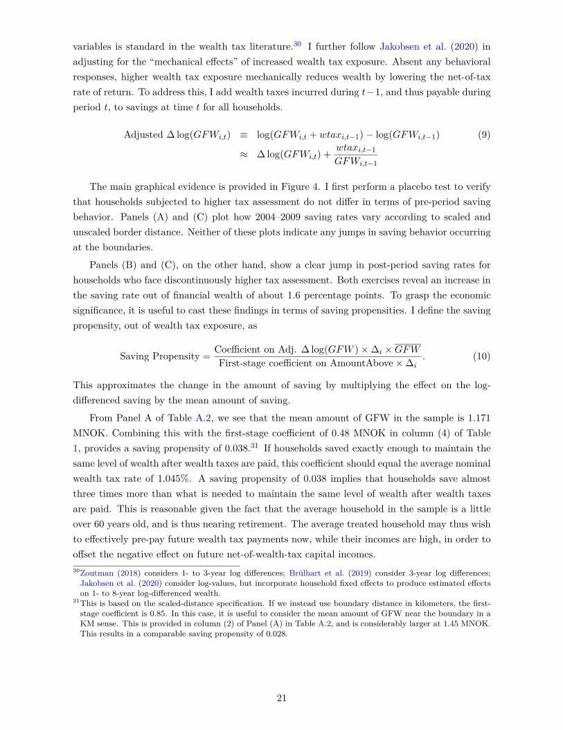
Adjusted ∆ log(GFWi,t) ≡ log(GFWi,t + wtaxi,t−1)− log(GFWi,t−1) (9)

≈ ∆ log(GFWi,t) + wtaxi,t−1GFWi,t−1

The main graphical evidence is provided in Figure 4. I first perform a placebo test to verifythat households subjected to higher tax assessment do not differ in terms of pre-period savingbehavior. Panels (A) and (C) plot how 2004–2009 saving rates vary according to scaled andunscaled border distance. Neither of these plots indicate any jumps in saving behavior occurringat the boundaries.

Panels (B) and (C), on the other hand, show a clear jump in post-period saving rates forhouseholds who face discontinuously higher tax assessment. Both exercises reveal an increase inthe saving rate out of financial wealth of about 1.6 percentage points. To grasp the economicsignificance, it is useful to cast these findings in terms of saving propensities. I define the savingpropensity, out of wealth tax exposure, as

Saving Propensity = Coefficient on Adj. ∆ log(GFW )×∆i ×GFWFirst-stage coefficient on AmountAbove×∆i

. (10)

This approximates the change in the amount of saving by multiplying the effect on the log-differenced saving by the mean amount of saving.

From Panel A of Table A.2, we see that the mean amount of GFW in the sample is 1.171MNOK. Combining this with the first-stage coefficient of 0.48 MNOK in column (4) of Table1, provides a saving propensity of 0.038.31 If households saved exactly enough to maintain thesame level of wealth after wealth taxes are paid, this coefficient should equal the average nominalwealth tax rate of 1.045%. A saving propensity of 0.038 implies that households save almostthree times more than what is needed to maintain the same level of wealth after wealth taxesare paid. This is reasonable given the fact that the average household in the sample is a littleover 60 years old, and is thus nearing retirement. The average treated household may thus wishto effectively pre-pay future wealth tax payments now, while their incomes are high, in order tooffset the negative effect on future net-of-wealth-tax capital incomes.30Zoutman (2018) considers 1- to 3-year log differences; Brulhart et al. (2019) consider 3-year log differences;

Jakobsen et al. (2020) consider log-values, but incorporate household fixed effects to produce estimated effectson 1- to 8-year log-differenced wealth.

31This is based on the scaled-distance specification. If we instead use boundary distance in kilometers, the first-stage coefficient is 0.85. In this case, it is useful to consider the mean amount of GFW near the boundary in aKM sense. This is provided in column (2) of Panel (A) in Table A.2, and is considerably larger at 1.45 MNOK.This results in a comparable saving propensity of 0.028.

21

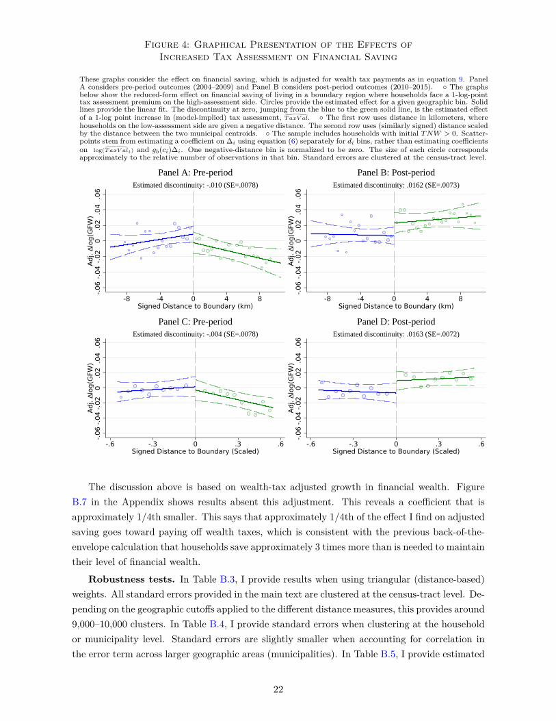
Figure 4: Graphical Presentation of the Effects ofIncreased Tax Assessment on Financial Saving

These graphs consider the effect on financial saving, which is adjusted for wealth tax payments as in equation 9. PanelA considers pre-period outcomes (2004–2009) and Panel B considers post-period outcomes (2010–2015). ◦ The graphsbelow show the reduced-form effect on financial saving of living in a boundary region where households face a 1-log-pointtax assessment premium on the high-assessment side. Circles provide the estimated effect for a given geographic bin. Solidlines provide the linear fit. The discontinuity at zero, jumping from the blue to the green solid line, is the estimated effectof a 1-log point increase in (model-implied) tax assessment, TaxV al

∧

. ◦ The first row uses distance in kilometers, wherehouseholds on the low-assessment side are given a negative distance. The second row uses (similarly signed) distance scaledby the distance between the two municipal centroids. ◦ The sample includes households with initial TNW > 0. Scatter-points stem from estimating a coefficient on ∆i using equation (6) separately for di bins, rather than estimating coefficientson log(TaxV al∧

i) and gb(ci)∆i. One negative-distance bin is normalized to be zero. The size of each circle correspondsapproximately to the relative number of observations in that bin. Standard errors are clustered at the census-tract level.

-.06

-.04

-.02

0.0

2.0

4.0

6Ad

j. ∆l

og(G

FW)


Estimated discontinuity: -.010 (SE=.0078)

Panel A: Pre-period

-.06

-.04

-.02

0.0

2.0

4.0

6Ad

j. ∆l

og(G

FW)



Panel B: Post-period

-.06

-.04

-.02

0.0

2.0

4.0

6Ad

j. ∆l

og(G

FW)



Panel C: Pre-period

-.06

-.04

-.02

0.0

2.0

4.0

6Ad

j. ∆l

og(G

FW)



Panel D: Post-period

The discussion above is based on wealth-tax adjusted growth in financial wealth. FigureB.7 in the Appendix shows results absent this adjustment. This reveals a coefficient that isapproximately 1/4th smaller. This says that approximately 1/4th of the effect I find on adjustedsaving goes toward paying off wealth taxes, which is consistent with the previous back-of-the-envelope calculation that households save approximately 3 times more than is needed to maintaintheir level of financial wealth.

Robustness tests. In Table B.3, I provide results when using triangular (distance-based)weights. All standard errors provided in the main text are clustered at the census-tract level. De-pending on the geographic cutoffs applied to the different distance measures, this provides around9,000–10,000 clusters. In Table B.4, I provide standard errors when clustering at the householdor municipality level. Standard errors are slightly smaller when accounting for correlation inthe error term across larger geographic areas (municipalities). In Table B.5, I provide estimated

22

effects when varying the location measure cutoffs for the scaled border distance measure, borderdistance in KM, and the relative location measure, respectively. Effects are qualitatively similarwhen varying the bandwidths, but tend to be larger (and more noisily estimated) the narrowerthe bandwidth.

Debt. The most intuitive way to save to offset future tax liabilities is arguably to increaseliquid (gross) financial wealth. This may may be particularly true for wealth-tax payers who tendto be wealthier and older and thus either hold less debt or be closer in time to having completedtheir debt repayments.32 Using the existing framework, I find no evidence of discontinuities in(either pre-period or) post-period debt accumulation Figure B.2 in the Appendix.

Taxable wealth. The focus on financial saving is motivated by the need to minimizemeasurement error arising from misreporting. However, it also removes measurement errorsarising from a broader wealth measure such as TNW that includes, e.g., the estimated value ofmotor vehicles. It would, for example, be particularly challenging to map estimated car valuedepreciation to saving behavior. Nevertheless, I consider the effects on TNW in section 6.2.3.This reveals a weakly positive effect, consistent with households responding by saving more whilenot simultaneously reducing other taxable assets.

4.4 Portfolio Allocation

4.4.1 Stock Market Share of Financial Wealth

In this section, I examine the effect of increased wealth tax exposure on the share of financialwealth allocated to the stock market. Portfolio allocation plays a key role in the dynamicsof wealth inequality (Martınez-Toledano, 2020); is important in understanding why wealthierhouseholds achieve higher returns (Bach, Calvet, and Sodini, 2020b); and both theory andevidence from the household finance literature suggest that the risky share of financial wealthmay be affected by a wealth-tax induced reduction in the rate of return.

As a theoretical benchmark, it is useful to consider constant relative risk aversion (CRRA)agents who allocate a fixed share of their life-time wealth to the stock market. Increased wealthtaxation, as in my empirical setting, largely lowers the future component of life-time wealth.Since current wealth remains largely unaffected, but stock holdings go down, we would expectthe stock market share of financial wealth to decrease.

However, there are two reasons why I would expect the stock market share to remain unal-tered. First, it is possible that the effect of increased wealth tax exposure on life-time wealth isfully offset by the behavioral responses that I document. Thus, if life-time wealth remains thesame, we would also expect the level of stock market holdings to remain fixed.

Second, there is the alternative view that households may respond to a tax-induced reductionin the risk-free rate by “reaching for yield” as in, e.g., Lian, Ma, and Wang (2019). Essentially,households may wish to offset the adverse effect on their portfolio-wide expected return by allo-cating more wealth to higher-expected-return assets. Relatedly, households may wish to allocatemore wealth to assets that yield higher income flows, which may entail unloading deposits or32The median household only has NOK 138,000 (USD 23,000) in debt (see Table A.1).

23

bonds in favor of dividend-paying stocks (Daniel, Garlappi, and Xiao, 2021).

I present my empirical results in Panel A of Figure 5. This plot reveals no change in thestock market share for households more exposed to wealth taxation. The associated confidenceinterval is [-0.0024, 0.0022]. A back-of-the-envelope calculation suggests that we can rule outa yearly increase in capital incomes above NOK 110 (USD 18).33 There is little evidence withwhich to compare these findings. While, for example, Alan, Atalay, Crossley, and Jeon (2010)find evidence that capital taxation affects portfolio allocation in Canada, their findings are drivenby a reallocation toward tax-favored assets. In contrast, the identifying variation in my settinghas no direct, differential effect on the returns on safe versus risky assets.

Figure 5: The Effects on Portfolio Allocation:Stock Market Share and Realized Pre-tax Returns on Safe Assets

These graphs consider the effect on (Panel A) changes in the stock market share (SMS), which is the ratio ofstock market wealth (SMW) to gross financial wealth (GFW) and (Panel B) changes in the realized interest rateson deposits. ◦ The graphs below show the reduced-form effect of living in a boundary region where householdsface a 1-log-point tax assessment premium on the high-assessment side. Circles provide the estimated effect fora given geographic bin. Solid lines provide the linear fit. The discontinuity at zero, jumping from the blue tothe green solid line, is the estimated effect of a 1-log point increase in (model-implied) tax assessment, TaxV al

∧

.◦ See Figure 4 for a full figure description. ◦ Figures B.3 and B.4 in the Appendix provide pre-period placeboresults and estimates based on the KM-distance specification.

-.02

-.01

0.0

1.0

2∆S

MS


Estimated discontinuity: -.00012 (SE=.001185)Panel A: Stock Market Share

-.002

-.001

0.0

01.0

02∆I

nter

est R

ate


Estimated discontinuity: -.00007 (SE=.000104)Panel B: Interest Rate on Deposits

4.4.2 The effect on realized returns on safe assets

I further consider the effect on realized returns on deposits. Instead of allocating morewealth to risky assets, households may exert more effort toward optimizing their risk-free return,which may cause wealth taxation to increase (pre-tax) return heterogeneity,34 and through it,wealth inequality (Bach, Calvet, and Sodini, 2017). The banking literature has documentedconsiderable dispersion in the (net-of-fee) interest rates on deposits (see, e.g., Azar, Raina, andSchmalz 2019). This large dispersion may be supported by switching costs that render thedeposit rates less competitive (Sharpe, 1997). I propose the hypothesis that households may33110 = 0.0022*1MNOK*5%. I multiply the upper bound of the confidence interval by the mean amount of GFW

(1MNOK) and by an assumed risk premium of 5% to obtain an estimate the effect on capital income.34See, e.g., Bach, Calvet, and Sodini (2020b) and Fagereng, Guiso, Malacrino, and Pistaferri (2020) who document

the extent of return heterogeneity across the Swedish and Norwegian wealth distributions.

24

choose to suffer these non-pecuniary costs, i.e., supply more effort, in order to offset the adverseeffects of more aggressive wealth taxation. I test this by considering the average realized returnson bank deposits,

Interest Rate on Depositsi,t = Total Taxable Interest Incomei,t0.5 ·Depositst−1 + 0.5 ·Depositsi,t

. (11)

I report the main result in Panel B of Figure 5. The evidence is inconsistent with myinitial hypothesis. Households’ realized returns appear quite unaffected by the wealth tax treat-ment.

As a benchmark, it is useful to establish what a hypothetical, large effect would be. TableA.1 shows that the difference between the 75th and 50th percentiles of the realized interestrate is 0.61 percentage points. If every household pushed above the threshold increased theirinterest rates by 0.61 percentage points, the estimated coefficient in Panel A should be around0.0014.35 This hypothetical effect is 26 times larger than the upper bound of the 95% confidenceinterval in Panel A. In other words, my findings are inconsistent with a substantial “searchingfor interest” channel. However, this does not imply that I can rule out scale dependence inreturns, which is discussed in the context of optimal capital taxation by Schulz (2021). This isbecause the behavioral saving response is likely too modest to trigger an increasing-returns-to-scale effect.

4.5 Reduced-form Effect of Wealth Taxation on Labor Earnings

In this subsection, I present results on how increased wealth tax exposure affects households’labor earnings,

Labor Earningsi,t = salary and wage earningsi,t + max(self-employment incomei,t,0). (12)

I focus on pre-tax labor earnings in the form of salary, wages, and self-employment income.This excludes other components of total taxable labor income (TTLI), such as pensions, thatare largely unaffected by concurrent labor supply but still endogenous (Brinch, Fredriksen, andVestad, 2018). Under the reasonable assumption of interconnected municipal labor markets,wages will not be affected in my setting. The implication is that changes to labor earnings mayserve as a proxy for labor supply.

Studying labor supply responses is particularly useful because it circumvents common mea-surement issues in studying the effects of wealth taxation on saving behavior. Firstly, householdlabor supply is not directly affected by incentives to misreport wealth. Secondly, it is not directlyaffected by how wealth taxation may encourage households to save in harder-to-tax (or easier-to-evade) asset classes such as art or durable consumption goods. Both of these phenomenamay cause a downward bias in the inferred effect on saving behavior. Focusing on third-partyreported financial saving will shut down the first bias in my setting. However, the propensity tosave in unobserved asset classes may still be affected.36

35This equals 0.61 p.p. times the first-stage coefficient on 1[TNW > Threshold] of 0.227936Although such spillovers are unlikely to be substantial, as the gains from such evasion or avoidance are limited.

25

Beyond addressing measurement issues, the effect on labor earnings is independently infor-mative of the EIS (see, e.g., the two-period model in section E in the Appendix). This stronglink between saving and labor supply responses to net-of-tax rate-of-return shocks implies thatunderstanding labor earnings responses becomes crucial for optimal taxation, as taxing capitalmay have first-order effects on revenues from taxing labor incomes.

Figure 6: The Effect of Wealth Taxation on Household Labor Earnings

These graphs consider the effect on labor earnings growth, ∆log(LaborEarnings). Labor earnings is defined as the sum ofsalaried and wage income as well as max(self-employment income,0). ◦ The graphs below show the reduced-form effectof living in a boundary region where households face a 1-log-point tax assessment premium on the high-assessment side.See Figure 4 for a detailed figure description. The pre-period (placebo) version of these graphs are provided in Figure B.5in the Appendix.

-.08

-.04

0.0

4.0

8∆l

og(L

abor

Earn

ings

)



Panel A: Distance in KM

-.08

-.04

0.0

4.0

8∆l

og(L

abor

Earn

ings

)



Panel B: Scaled Distance Specification

Figure 6 shows the main results, using both the km and scaled distance specifications. Wesee that labor earnings decrease somewhat as we move toward and into the high assessmentsides of the boundaries. However, at the assessment discontinuities, household labor earningsgrowth jumps by about 1.9-3.3 percentage points. In order to relate these findings to the effecton saving behavior, I define an earning propensity, similar to the saving propensity in equation(10). Since labor earnings is a flow variable, and I am considering the effect on its growth rate,I cumulate the growth over a 5-year period, and divide again by 5 to obtain an average-earningpropensity.

Earning Propensity = 15

∑5t=1 t× Coef. on ∆ log(LaborEarnings)×∆i × LaborEarnings

First-stage coefficient on AmountAbove×∆i. (13)

I obtain the benchmark levels of Labor Earnings of 0.659 and 0.588 MNOK from Table A.2 forhouseholds near the boundary in a KM- and scaled-distance sense, respectively. I divide by therespective effects on the amount of wealth above the threshold of 0.846 and 0.477 MNOK. Thisprovides pre-tax earnings propensities of 0.060 and 0.054. Assuming a marginal tax rate of 50%leads to after-tax earnings propensities of 0.030 and 0.027. These are similar in magnitude to the

For example, evaded cash would still underperform deposits by the difference between the average rate ondeposits (2%) and the nominal wealth tax rate (about 1%). Other assets, such as art may be easy to evade,but carry much more risk than, e.g., deposits or bonds, and is particularly illiquid.

26

saving propensity that I uncovered earlier, suggesting that a large part of the increase in yearlysaving is financed by increased labor supply. Of course, there will be estimation error bothabove and below the numerator which precludes me from putting narrow intervals this ratio ofpropensities. However, this exercise shows that labor supply may be an important margin ofadjustment for households facing more aggressive capital taxation.

4.6 Boundary Discontinuity Estimates With Different Specifications

In this section, I discuss how the main reduced-form results vary depending on which specifi-cation is used. The underlying regression estimates are presented in Appendix Table B.6, whereeach column represents different approaches to address geographic heterogeneity.

The first column ignores unobserved geographic heterogeneity. The second column intro-duces boundary area fixed effects, and thus compares households in adjacent municipalities ordistricts in the four largest cities. We can see that the point estimates do not change much whenadding these fixed effects. This is likely due sosio-economic control variables already absorbing alarge part of this variation. Columns (3)-(5) introduce geo-coded control variables that accountfor unobserved heterogeneity within a boundary area. For most of the outcome variables, we seethat this does not materially change the estimated coefficients relative to column (2) where onlyboundary area fixed effects were included. This is not surprising given the graphical evidencepresented in the previous subsections that show how the estimated discontinuities correspondto the differences in means across the boundaries.

Introducing geo-coded control variables do have a substantial impact on the estimated effecton debt, however. Columns (1) and (2) both wrongly suggest that higher wealth tax expo-sure leads to more debt accumulation. Figure B.2 in the Appendix, show that this is drivenby a gradual increase in debt accumulation as we move into the high-assessment side of theboundary. This figure also shows how using a differences-in-differences design, rather than aboundary-discontinuity design, would exacerbate this problem. In the pre-period, householddebt accumulation is decreasing in border distance; a differences-in-differences approach wouldthus produce large positive effects on debt accumulation. While columns (3)-(4) show that theKM and scaled-distance specifications generally agree on the coefficients, the KM-specificationsuggests a larger effect on labor earnings. However, when accounting for the fact that the KM-specification is associated with a higher first-stage effect, the implied earnings propensities arealmost identical.37

4.7 Year-by-year Effects

When estimating the discontinuities year by year, I find that treatment effects are quitesimilar over time. This is a useful exercise to inform the mechanism behind the observed savingresponses. For example, Zoutman (2018) finds that his estimated elasticities are driven by37When drawing households near the boundary in a KM sense, we are more likely to draw households from more

densely-populated, higher-income areas. These boundary areas have higher average house price levels, whichcauses a given relative increase in tax assessment to have a larger effect on wealth tax exposure measured in theamount of wealth above the threshold. See calculations of earnings propensities in the preceeding subsection4.5 and the discussion surrounding the first-stage effects in subsection 4.2.

27

rather immediate responses. He therefore attributes the high elasticity to changes in reportingbehavior, since real responses arising from changes in consumption and labor supply will likelyoccur gradually. Below, I show that the main estimates are not driven by a single year, whichis consistent with real responses caused by gradual consumption and labor supply adjustments.These findings are provided in Figure B.8 in the appendix. While there is some variation in theeffect on the growth rate of debt over time, we see that it is zero on average, and eventuallygoes negative, consistent with a positive effect on net saving.

4.8 The Effect on House Prices and the Propensity to Sell

In this subsection, I report my findings on the effect on whether households subject to higherwealth tax exposure move, and whether more highly-assessed houses sell for less. These resultsare provided in Table B.1 in the Appendix.

Propensity to sell. Panel A of Table B.1 finds no effect on the propensity to sell. Sincetax assessments stay with the house, households may “untreat” themselves by selling their houseand moving to an area with lower assessments. I do not believe that this is likely, given myimpression of limited awareness of the detailed geographic aspects of the pricing model, aswell as the likely presence of sizable costs associated with moving. Consistent with this, I findstatistically small effects on the propensity to sell. The estimates using the main, scaled-distancespecification shows that a 1-log-point increase in TaxV al

∧

increases the likelihood of selling byonly 0.2 percentage points. I can rule out any effects larger than 0.8 percentage points at the5% significance level.

Subsequent transaction prices. Panel B of Table B.1 finds no effect on conditional salesprices. The effect of increased tax assessment (which follows the house) on tax prices likelydepends on the propensity of potential buyers to be subject to a wealth tax. Since most newhomeowners finance their purchases with debt, the net effect of a house purchase on their TNWis highly negative. This is because debt is deducted from TNW in its entirety, while the taxvalue of the house, on average, corresponds to around 25% of its market value. This causesnew home buyers to generally have very low (negative) TNW. Any tax assessment premiumsare therefore unlikely to affect these households’ immediate wealth tax liabilities, lowering thedemand side’s sensitivity to the tax assessments. Consistent with this, I find no statisticallysignificant effect on subsequent sales prices. The estimated point estimates from the preferredspecifications in columns 1 and 3 are rather small, at 0.035 and 0.016, and not statisticallydifferent from zero.

Even if there were an effect on house prices, this would not produce income or wealth effectson top of the income effects associated with facing higher future wealth tax bills. This is becausethe housing wealth effect would only materialize if there is a sale, in which case the standardwealth-tax income effect seizes. Thus, we think of a potential house price capitalization effect assimply rendering moving away futile with respect to undoing the wealth-tax treatment.

28

4.9 Regression-based Analysis of Pre-treatment Differences

In this subsection, I explore whether my identifying variation in wealth tax exposure, arisingfrom geographic assessment discontinuities, is correlated with pre-period observables.

Table 2: The Correlation Between Treatment and HouseholdCharacteristics after Including Geographic Controls

This table reports the correlation between model-implied tax assessment, log(TaxV al∧

), and 2009 socioeconomic char-acteristics: Income, GFW, debt, and education. College is a dummy equal to one if any of the household adults havea college degree. Columns (1)-(4) add different sets of controls. Column (1) includes the baseline controls: structure-type-specific slopes on log(size), the dense population dummy, and age bracket indicators. Column (2) interacts thebaseline controls with border area fixed effects. Column (3) further includes a control for the distance to border withina border area, estimated separately for each side, and interacted with ∆i (border area and structure-type-specificlog(difference) in average assessed house prices between the sides of the border). Column (4) includes the relativelocation control, also interacted with ∆i. These two variables are defined in detail in the text. Standard errors areprovided in parentheses, and are clustered at the census-tract level. Sample sizes are provided in brackets.

(1) (2) (3) (4) (5)No geo. Boundary FEs KM Distance Scaled Distance Rel. Location

log Past Transaction Price, Post-2000

log( TaxV al) 1.461*** 0.776*** -0.064 -0.061 -0.112(0.040) (0.110) (0.244) (0.224) (0.211)[40310] [39748] [39748] [38728] [38728]

log Past Transaction Price, Post-2004

log( TaxV al) 1.494*** 0.943*** 0.251 -0.095 -0.442(0.071) (0.172) (0.333) (0.335) (0.323)[18062] [17469] [17469] [17073] [17073]

log Total Taxable Labor Income in 2009

log( TaxV al) 0.288*** 0.153*** 0.067* -0.000 0.002(0.005) (0.013) (0.040) (0.028) (0.023)[261300] [260774] [260769] [236241] [254364]

log Gross Financial Wealth in 2009

log( TaxV al) 0.629*** 0.409*** 0.255*** -0.030 0.002(0.012) (0.035) (0.095) (0.070) (0.064)[261300] [260774] [260769] [236241] [254364]

Stock Market Share in 2009

log( TaxV al) 0.045*** 0.028*** 0.053*** 0.000 0.002(0.002) (0.005) (0.014) (0.010) (0.009)[261139] [260612] [260607] [236096] [254208]

log Debt in 2009

log( TaxV al) 0.502*** 0.350*** 0.180 0.092 0.097(0.015) (0.046) (0.143) (0.099) (0.082)[261300] [260774] [260769] [236241] [254364]

College Degree

log( TaxV al) 0.239*** 0.194*** 0.159*** 0.019 0.028(0.005) (0.015) (0.040) (0.028) (0.024)[260599] [260075] [260070] [235610] [253687]

Controls

Household Characteristics Yes Yes Yes Yes YesHousing Characteristics Yes Yes Yes Yes Yes– Border specific – Yes Yes Yes Yes

Border Distance Controls– KM, KM2 – – Yes – –– Scaled – – – Yes –Relative Location Controls – – – – Yes

29

The first variable that I consider in Table 2 is past transaction prices. While the hedonicpricing model is estimated on transactions after 2004, I also include the years 2000–2003 in thefirst row, in order to increase precision. In the second row, I restrict my analysis to transactionsafter 2004. Column (1) shows that houses in higher-assessed areas are indeed more expensive.38

This strong positive relationship persists when I control for boundary area fixed effects, withgreatly limits the potential amount of geographic heterogeneity. However, these differences losetheir significance once I address within-boundary-area heterogeneity in columns (3)-(5). This isconsistent with the visual evidence in Figure 2 where past transaction prices are plotted againstthe distance measures.

In terms of point estimates, it is the scaled distance measure in column (4) that estimates thesmoothest price path across the boundary. Given the fairly nonlinear relationship between ex-ante observables and border distance in kilometers presented Figure 2, I allow for a more flexible,second-order relationship in the regressions underlying Table 2. This is mainly to give it moreof a fighting chance against the preferred scaled-distance specification in column (4).

Since there is no indication of jumps in past transaction prices at the assessment boundaries,it is not surprising that the subsequent rows reveal no discontinuities in other socioeconomiccharacteristics. If house prices are in fact smooth across geographic boundaries, it is reasonableto expect that other household characteristics are as well. Table 2 shows that the identifyingvariation in log(TaxV al∧

) is uncorrelated with past incomes, financial wealth, portfolio allocation,debt, as well as educational attainment, when geographic heterogeneity is accounted for withthe scaled-border specification in column (4). We see that the relative location measure alsoperforms particularly well, but that the kilometer specification struggles. This is reasonablegiven what we saw earlier in Figure 2, that the relationship between 2009 incomes and border-distance in kilometers is highly nonlinear.

5 The Implied EIS in a Simple Life-Cycle Model

The degree to which economic agents are willing to substitute consumption across periodsis one of the most important modeling choices in economics. In standard models, this choice isreflected in the Elasticity of Intertemporal Substitution (EIS) or, equivalently in models withno uncertainty, the inverse of the coefficient of relative risk aversion. While the central role ofthe EIS in macroeconomic models is well appreciated, its importance in public finance may havebeen obfuscated by the classical result that, regardless of the EIS, the optimal long-run tax rateon savings is zero (Chamley 1986 and Judd 1985).39 Recently, however, this result has beenoverturned by Straub and Werning (2020) in the same models in which it arose. Whether itis optimal to tax capital does indeed depend crucially on the EIS in classical models. In thissection, therefore, I use a simple life-cycle model to examine which value of the Elasticity ofIntertemporal Substitution (EIS) is most consistent with my empirical findings.38It should be noted, however, that this does not verify the ability of the hedonic pricing model to price houses

out of sample, as these transactions would have been included in the model’s estimation sample.39Of course, multiple studies outline settings in which capital taxation is indeed optimal. See, for example,

Diamond and Spinnewijn 2011.

30

The model environment is simple: It only contains the core elements necessary to replicatemy empirical results and the shock to wealth tax exposure. Agents choose both how much to saveand how much to work, and importantly, they’re shocked by more aggressive wealth taxationin such a way that the effect on the marginal and average net-of-tax rates-of-return may differ.The model environment accounts for the fact that the average household in my sample is close toretirement and thus faces lower incomes in the near future. To simplify the analysis, I abstractfrom frictions, but discuss how they may play a role in interpreting the mapping between myempirical findings and the EIS.

5.1 A simple life-cycle model

Consider the following life-cycle model with perfect foresight. The model features a constantEIS, 1

γ , and a constant Frisch elasticity of labor supply, 1ν .

max{ct,st+1,lt}Tt=0

∑Tt=0 βt

(1

1− γ c1−γt − ψ l1+ν

t

1 + ν

), (14)

s.t. ct + st+1 = yt + ltwt (15)

+ stR− wtaxt(st).

ψ is the (dis)utility weight on labor supply, and β is the time discount factor. Households choosehow much to consume, ct, work, lt, and save, st+1 each period. Unearned income (pensions), ytand initial wealth, s0, are exogenous. Households earn a gross rate of return of R, but must paywealth taxes, wtaxt, that depend on st.

Agents face a wealth tax schedule where any savings, st, in excess of the threshold, s, issubject to a tax rate of τ , according to the following formula.

wtax(st) = (st − s)1[st > s]τ. (16)

Rewritten budget constraint. Now define MTRt = 1[st > s]τ and ATRt = wtax(st)/st.This allows us to rewrite the budget constraint as

ct + st+1 = yt + ltwt + st(R−MTRt

)︸︷︷︸Linearized GrossCapital Income

+ st(MTRt −ATRt

)︸︷︷︸Virtual Income

, (17)

where the second-to-last term is the gross, net-of-wealth-tax capital incomes the agent wouldobtain if there were no wealth tax threshold. Since there is such a threshold, the last termcontains the necessary virtual-income compensation. This decomposition allows for a straight-forward mapping between my first-stage estimates and the shocks to the budget constraintexperienced by the life-cycle agent.

31

5.2 Calibration

In my main specification, I follow Jakobsen et al. (2020) in modeling the responses of arepresentative agent. I set R = 1.02. The baseline MTR and ATR are both set to zero. Theunshocked (counterfactual) agent sees no changes to MTR or ATR. The shocked agent sees theirMTR shocked by dMTR, which equals the empirical first-stage estimate on MTR in Table 1.Since I model the responses in terms of GFW , the shocked agent sees dATR = dATRGFW

∧

. Thisis the first-stage coefficient on the average tax rate relative to GFW,ATRGFW = wtaxi,t/GFWi,t,which is reported in Table B.12. The virtual income shock is set to s′t(dMTR− dATR), wheres′t is the simulated savings path of the unshocked agent.

I simulate the responses in terms of their saving behavior and labor supply for EIS-Frischcombinations, ( 1

γ ,1ν ). I set β = 0.96. The (dis)utility weight on labor supply, ψ, is calibrated to

ensure that simulated labor earnings at t = 0 equal observed after-tax labor earnings, assumingan average income tax rate of 0.3, and that the consumption share of total incomes (laborearnings plus exogenous income) equals 80%.40

The role of the exogenous income, yt, is to imitate pension income. For agents below anominal retirement age of 65, I set this equal to the difference between mean total taxable laborincome and labor earnings that I observe in the data. Once agents reach nominal retirementage, yt increases by 60% of the average observed labor earnings. Pensions are then taxed ata linear rate of 0.3. This procedure accounts for some households in the data already beingretired before the age of 65. I induce agents to retire by making wages drop to zero over a 5-yearperiod that starts at age 65. To simplify the analyses, I do not model bequests motives directly.Instead, I assume that households live until they are 100 years old and do not receive pensionincomes after age 90. This ensures that households do not dissave too quickly, and thereforestill hold meaningful savings around the average (empirical) age of death in Norway, which isaround 85 years.41

5.3 Simulated Treatment Effects

Figure 7 shows simulated treatment effects for different values of the EIS. Panel A considersthe effect on the growth rate of financial saving absent the wealth tax adjustment (correspondingto the empirical findings in Figure B.7). We see that the cut-off for when we see a change inthe sign of the saving response is around 0.45. This is lower than the canonical cut-off of 1in a pure-capitalist model due to human wealth effects offsetting the income effect (Elmendorf,1997). The figure shows that an EIS of about 0.02–0.08 can replicate my empirical findings.This is only moderately dependent on the Frisch elasticity of labor supply. We see that savings40Choosing a consumption share of 80% ensures that agents choose labor supply close to the empirical average

in the sample. Setting it to 100%, for example, leads to very large (unshocked) labor supply in order to saveenough to finance a higher level of consumption.

41Absent any mortality risk, this roughly corresponds to (1) assuming that the bequest elasticity equals the EIS,and (2) that the strength of the (warm-glow) bequest motive ensures that households wish to bequeath anamount large enough to finance their own planned consumption for 15 years. If instead agents ended theirlife-cycle at age 85 with zero residual assets, income effects would be weaker, and even lower values of the EISwould be needed to obtain simulated treatment effects consistent with the confidence intervals on my empiricalfindings.

32

growth is somewhat more responsive when labor supply adjustments are less costly, i.e., whenthe Frisch elasticity is higher. However, as long as it is sufficiently positive, the Frisch elasticityplays a modest role in mediating the responses.

Figure 7: Simulated Treatment Effects as a Function of the EIS

This figure shows the relationship between simulated saving and labor earnings responses and the Elasticity of IntertemporalSubstitution (EIS). The long-dashed green lines provide the empirical point estimates, with surrounding 90% and 95%confidence intervals. The solid blue line provides the simulated treatment effect for different values of the EIS when theFrisch elasticity, 1/ν, is 0.25. The dashed blue line uses a Frisch elasticity of 1.25. Panel A considers financial savingsgrowth, without the wealth tax adjustment, where the empirical point estimate comes from Figure B.7. Panel B considerslabor earnings growth, where the point estimate comes from Panel B of Figure 6. The citations in grey correspond toexisting estimates of the EIS. Best et al. 2020 estimate an EIS of 0.1. Havranek 2015 finds that the mean of existingestimates is 0.5. The calibrated EIS in Jakobsen et al. 2020 ranges from 2 to 6. Figure B.9 in the Appendix repeats thisexercise while allowing for first-stage heterogeneity. When Frisch=0.25 (1.25), the lowest computationally feasible EIS was0.0088 (0.02). Simulated effects are smoothed by using a local 5th-order polynomial fit.

Best, Cloyne, Ilzetzki, and Kleven (2020)

Havránek (2015) Mean EIS, meta-study

Jakobsen, Jakobsen, Kleven, Zucman (2020)

-.06

-.03

0.0

3.0

6Δ

log(

GFW

), An

nual

ized

0 .25 .5 .75 1EIS

Empirical (with 90-95% CI)Simulated (Frisch = 0.25)Simulated (Frisch = 1.25)

(A) Financial Savings Growth

-.04

-.02

0.0

2.0

4.0

6.0

8Δ

log(

Labo

rEar

ning

s), A

nnua

lized

0 .25 .5 .75 1EIS


(B) Labor Earnings Growth

This figure also shows that empirically finding positive saving responses to wealth taxation is

33

not too surprising. For example, the EIS of 0.1 found by Best, Cloyne, Ilzetzki, and Kleven (2020)produces simulated saving responses that are statistically indistinguishable from my empiricalfindings. The same applies to recent evidence from India and Japan, where the EIS is foundto be 0.022 (Agarwal, Chua, Ghosh, and Song, 2020) and 0.21 (Cashin and Unayama, 2016).While there is little U.S. evidence, recent work by Baker, Johnson, and Kueng (2021) finds thatan EIS of 0.19 best explains long-run responses to variation in sales taxes. Havranek (2015)reviews existing estimates of the EIS more broadly and finds a mean of 0.5, but considerabledispersion. While this suggests that a large swath of empirical estimates are consistent withmy estimated treatment effects, Havranek (2015) points out that the mean microeconometricestimates published in Top-5 journals is close to 1.42 From this, I would draw the conclusionthat my findings are not inconsistent with previous empirical evidence, as the existing empiricalevidence itself is far from consistent.

It is also useful to consider values of the EIS derived from wealth taxation. Jakobsen,Jakobsen, Kleven, and Zucman (2020), using different identification strategies, find that theimplied EIS ranges from 2 to 6. Values of the EIS that are this large are clearly not reconcilablewith my empirical evidence. However, they are also not inconsistent, as Jakobsen et al. (2020)emphasize that their calibrated EIS may be driven by evasion or avoidance. My empiricalevidence is further largely consistent with values of the EIS used in recent research using aquantitative macro models to consider the effects of wealth taxes: e.g., Broer, Kohlhas, Mitman,and Schlafmann (2021) who use an (implied) EIS of 0.2 and Rotberg and Steinberg (2021) whouse 0.25.

Panel B considers the effect on labor earnings. To map the simulated responses to thosefound in Panel B of Figure 6, I consider the cumulative labor earnings response, which I averageover time.43 Interestingly, labor earnings responses are almost as sensitive to EIS as the savingsresponses. The EIS cut-off below which we see positive earnings responses is only slightly higherat about 0.5. In order to replicate the empirical treatment effect, I need an EIS of about0.05–0.15. This range overlaps considerably with the one for savings responses.

First-stage heterogeneity. Figure B.9 shows results when incorporating first-stage hetero-geneity. This produces a qualitatively and quantitatively similar relationship between treatmenteffects and the EIS. I incorporate first-stage heterogeneity by allowing the first-stage coefficientson MTR and ATRGFW to vary by which 2009 quartile of TNW a household belongs to. Thesecoefficients, and summary statistics by quartiles, are provided in Table B.12. This exercisethus accounts for the fact that high TNW households on average saw a modest effect on their42There is considerable spread in assumed values of the EIS in quantitative modeling as well. For example, while

Guvenen (2009) uses an EIS between 0.1 and 0.3, Kaplan and Violante (2014) assume a value of 1.5.43In the simple model used for simulating treatment responses, labor supply responses are immediate. This is

because labor supply is determined through the intratemporal first-order conditions, which leaves the level oflabor earnings log-proportional to consumption. The adjustment to increased taxation thus comes immediatelyas the level of consumption is decreased. This differs from my empirical findings, in which household laborearnings growth is affected smoothly across time. This may be caused by households readjusting at differentpoints in time, or that households have a preference for smoothing labor supply adjustments. Since it is unclearhow to model labor supply adjustments in a way that produces a smooth response over time, I take the followingsimpler route. I calculate the cumulative, simulated labor earnings response, and then calculate the average, asif responses occurred smoothly over time.

34

marginal tax rates.

Credit constraints. If households were financially constrained, they would wish to front-load consumption more than they are already doing. In other words, they have an unmetpreference for dissaving. This would clearly mute substitution effects, as households are alreadyunable to dissave more. However, it would also work against finding large income effects. Posi-tive income effects on observed saving behavior would only materialize to the extent that theyexceed the pre-existing unmet demand for dissaving. Essentially, the income effects would haveto change the optimal saving path enough to render the agent unconstrained. This becomesproblematic to the extent that there is considerable EIS heterogeneity (which runs counter tothe findings in Best et al. 2020). In that case, credit constraints would fully mute the responsesof high-EIS households and only allow us to observe partially-muted responses of low-EIS, high-income-effect households. However, this is hard to square with my empirical findings for a fewreasons.

Firstly, treated households are fairly old and thus face declining income paths. This isat odds with material credit constraints for rational agents, since it is unclear against whatfuture incomes they wish to borrow against. Second, the households in my sample have ampleliquidity. Even at the 25th percentile, households hold NOK 224,000 (USD 37,000) in financialwealth out of which NOK 152,000 (USD 25,000) is in deposits (See Panel A of Table A.1). Goingfurther toward the left tail of the liquidity distribution, I find that only 6-7% of households haveless than NOK 50,000 (USD 8,333) in GFW, and that wealth taxes only exceed one quarterof GFW for about 0.2% of my sample (See Panel A of Table A.2). These statistics do notmaterially change when instead considering households positioned to experience larger shocks.It is therefore unlikely that financial frictions play an important role or that taxation inducesfinancial hardship as in Wong (2020).

Frictions to adjusting consumption. This section shows that in a simple life-cycle model,we need a fairly small value of the EIS to rationalize the empirical findings. We could alsoreplicate low-EIS behavior by exogenously imposing consumption adjustment frictions (Chettyand Szeidl, 2007). As a very simple example, consider the requirement that ct ≥ c0 for t ≥ 1. Insuch an environment, the responses to wealth taxation become uninformative of the EIS. Thefact that I cannot statistically rule out that increases in savings are fully paid for by increasedlabor earnings (rather than downward adjustments to consumption) lends support to such aneconomic environment. However, perhaps more reasonably, the strength of consumption frictionsare reduced over time. In that case, the presence of consumption frictions would still allow me todetect responses consistent with a high EIS: If the EIS is high (and thus the substitution effectis strong), households would want to shift more consumption from the future. If consumptionfrictions don’t bind in the future, households would optimally shift consumption toward thepresent by dissaving. My finding of a positive effect on saving behavior is inconsistent withthis.

35

6 Disentangling Marginal and Average Tax Rate Effects

The previous section used a standard life-cycle model to show that a small EIS is necessaryto rationalize my empirical findings. The negative relationship between the EIS and the savingand labor supply responses is a built-in feature in standard life-cycle models. This is becausethe EIS determines the strength of intertemporal substitution effects. By lowering the EIS, welower the substitution effects, and thereby allow income effects to dominate. The underlyingmechanism dictates that the substitution effects are driven by changes in the marginal net-of-taxrate of return, while income effects are driven by changes in the average net-of-tax rate.

In this section, I decompose the effects of increased wealth tax exposure into the effects ofchanging the marginal (MTR) and average tax rate (ATR) on wealth. This allows me to directlytest the mechanisms underlying the life-cycle model. First, an increase in the MTR lowers themarginal net-of-tax rate one for one, and should thereby cause dissaving. Second, an increase inthe ATR lowers the average net-of-tax rate, and should cause more saving. Since my empiricalresults indicate a combined effect that is positive, I should find MTR effects that are smaller inmagnitude than the ATR effects.

The gist of the exercise is that I use pre-period characteristics to create new variables thatpredict the extent to which geographic discontinuities in TaxV al change households MTRsversus ATRs. I then use these variables, interacted with the geographic discontinuities, asinstruments in an instrumental variables approach. This allows to separately identify the ef-fects.

6.1 Two Variables that Differentially Predict Extensive and Intensive-marginEffects of Assessment Discontinuities

The following expression provides the amount of wealth taxes a household must pay followinga relative increase in TaxV ali,t of δ.

wtax(δ)i,t = max(TNWi,t + δ · TaxV ali,t − Tt, 0). (18)

Now consider the following two empirical moments. These tell us the conditional marginaltax rate contribution (MTC) and the average tax rate contribution (ATC) of a 100%-increasein tax assessment. This is calculated by linearizing the effect around the given δ, which equals0.25 in the main specification. These conditional expectations (sample means) are functions ofthe conditional joint distribution of TNWi,t and TaxV ali,t. Conditional means are calculatedseparately for each year, t.

MTCt(δ∣∣Wi,2009) = 1

δEt[τt(1[wtax(δ)i,t > 0]− 1[wtax(0)i,t > 0]

) ∣∣∣Wi,2009], (19)

ATCt(δ∣∣Wi,2009) = 1

δEt[(wtax(δ)i,t − wtax(0)i,t)

/TNWi,t

∣∣∣Wi,2009]. (20)

When these two expressions are the same, assessment shocks induce rate-of-return changes that,on average, resemble those of a linear (e.g., capital income) tax. When MTC is substantially

36

larger than ATC, assessment shocks tend to lead to marginal (short-term compensated) returnshocks.

There are two natural choices for the set of conditioning variables, Wi,2009. The first is isTNWi,2009 due to persistence in wealth levels. The second is the tax assessment householdswould see absent the existence of an assessment discontinuity in their boundary area, TaxV al≈i

∧

.This counterfactual assessment is based on 2009 housing characteristics, Hi,2009, and is theaverage of the counterfactual low- and high-side tax assessments.44 The larger this counterfactualassessment is, the larger is the impact of a δ-increase on TNWi,t.

Conditioning on the predetermined TNWi,2009 and TaxV al≈i

∧

ensures that the conditionaljoint distribution of (TNWi,t, TaxV ali,t) is not affected by the assessment discontinuity. I furtheraccount for the fact that TNW growth rates likely depend on age and income levels by alsoconditioning on age and household income as of 2009. More specifically, I assign householdsinto one of 2,700 bins that are made up of 30 TNW2009 bins, 10 TaxV al≈

∧

bins, 3 income bins,and 3 age bins. Wi,2009 then indicates membership in a combination of these bins. While allgroups include more than one hundred household, and typically substantially more, I strengthenexogeneity by calculating conditional means using the leave-me-out method. For each individualhousehold, i, this method calculates means under the assumption that i does not belong to theirown group.

Figure 8: Effects of Higher Tax Assessment onMarginal and Average Wealth Tax Rates

This figure shows the tax-driven effect of increasing housing assessments on the marginal tax rate (MTC, bluecircles) and average tax rate (ATC, orange squares), and how this varies according to 2009-valued TNW. Theseare calculated as in equations (19) and (20). The frequency count (gray bars) corresponds to the right-hand-sidey-axis.

020

4060

80Fr

eque

ncy

(100

0s)

-20

020

4060

Chan

ge in

Tax

Rat

es (B

asis

Poi

nts)

-6000 -3000 0 3000 6000 9000 12000Taxable Net Wealth (TNW) in 2009, NOK 1000s

Marginal Tax Contribution (MTC)

Average Tax Contribution (ATC)

Figure 8 illustrates how the resulting MTCs and ATCs covary with TNW2009 by averaging44More specifically, this may be written as TaxV al≈i

∧

≡(TaxV ali∧∣∣

di<0+ TaxV ali∧∣∣

di>0

)/2

37

over non-TNW characteristics. We see that for TNWi,2009 < −2 000 000, the two lines are verysimilar, and close to zero. This means that very low-TNW households’ wealth tax exposure werenot significantly affected during 2010–2015. For higher TNW , there is initially a more rapidincrease in MTC than ATC. These are households who are likely to be pushed above, but notfar above, the wealth tax threshold. This implies that these households are likely to experiencea larger effect on marginal than average tax rates. For TNWi,2009 > 1, 000, 000, we see a slightdecrease in ATC and a rapid decrease in MTC. These are households who are likely to be—andstay—above the tax threshold even without an increase in tax assessment. These householdsare thus unlikely to see an effect on their marginal tax rates, but will see a full impact on theiraverage tax rates as more of their wealth is taxed on the intensive margin. The slight decreasethat we observe is caused by the fact that TNW rises faster than TaxV al, which means thata given percentage point increase in assessment has a decreasing effect on the ratio of wealthtaxes to TNW.

6.2 IV Methodology to Distinguish Between MTR and ATR Effects

This subsection describes how the two variables, MTC and ATC, are used as interactionvariables to obtain first-stage heterogeneity in how households’ MTR and ATR are affected. Inan IV framework, I can then separately identify the effects of changing average versus marginaltax rates.

While the previous analyses in section 4 only included households with initial TNW > 0,I now also include households with initial negative TNW. As Figure 8 shows, there is a largenumber of households with initial TNW ≤ 0 for whom MTRs should be non-trivially affectedby an inflated TaxV al.

My IV specification is built on, and uses the same notation as, the reduced-form regressionequation (6). There are two endogenous variables, MTR and ATR. The instrumental variationis obtained from interacting the assessment discontinuity term with zti = {MTCti , ATC

ti}. These

variables have superscript t, as they account for changes in the wealth tax threshold and nominaltax rate over time. I include zti interacted with the slope terms, as well as the potential increasein tax assessment, ∆i, as controls. I also include year-specific controls in zti. All coefficientsare estimated separately for households initially below and above the threshold (indexed bya), which ensures that the residualized geographic variation in saving behavior documented inSection 4 is unaltered.

wi,t = βwa,w∆i1[di > 0]′zti +gb,a,w(ci)∆izti + ξwa ∆izti + ρwt,azti (21)

+δ′b,s,a,wHi + γ′t,a,wXi + εwi,t, for w ∈ {MTR,ATR},

yi,t = βMTRMTRi + βATRATRi +gb,a(ci)∆izti + ξa∆izti + ρt,azti (22)

+δ′b,s,aHi + γ′t,aXi + εi,t.

This type of analysis is based on Gruber and Saez (2002). My primary innovation to thisapproach is to exploit persistent, differential tax exposure that arises due to tax assessmentdiscontinuities. The secondary innovation is to use the information from the conditional distri-

38

bution of TNW to enhance precision rather than assuming that TNW remains constant whenconstructing my instruments. This allows me to obtain a stronger instrument by accounting for,e.g., the extent to which TNW tends to rise for young high-income households but decline forthose that are older and lower income.

6.2.1 Saving Behavior and Labor Earnings

I provide the main results from estimating the system of equations (21)-(22) in Table 3. TheseIV analyses all use the main, scaled border distance specification. Columns (1)-(3) consider themain wealth-tax adjusted financial saving measure. Column (1) estimates the effect of changingMTR alone, using only the MTC interaction as the instrument. This reveals virtually no effecton saving behavior. Column (2) similarly only estimates the ATR effect. This shows a positiveeffect on saving, albeit not quite statistically significant, with a t-statistic of 1.5. Column (3)jointly estimates MTR and ATR effects. This shows a larger, and highly significant sensitivity ofsaving to the average tax rate. The sensitivity of saving to the marginal rate is now found to benegative, but insignificant, and small relative to the ATR effect. The increase in the magnitudeof both the estimated coefficients is consistent with theory ascribing opposite effects, and thefact that changes in MTR and ATR changes are positively correlated.

Table 3: Differential Saving and Labor Earnings Responsesto Changing Marginal and Average Tax Rates on Wealth

This table reports IV estimates of the effect of changing the marginal (MTR) and average tax rates (ATR) on savingbehavior and labor earnings. The IV specification is provided in equations (21)-(22). Columns (1)-(3) consider financialsaving adjusted for wealth tax payments, log(GFWi,t + wtaxi,t−1) − log(GFWi,t−1). Columns (4)-(6) consider log-differenced labor earnings, ∆ log(Labor Earnings). Geographic assessment discontinuities, 1[di > 0]∆i, interacted withMTCti and ATCti are used as instruments. MTCti and ATCti are based on 2009 observables and time t tax rules to providethe simulated impact of tax-assessment increases on MTR and ATR. The estimation sample also includes households withTNWi,2009 < 0; and all coefficients, on instruments and control variables, are allowed to vary by whether TNWi,2009 > 0.ATR + MTR provides the sum of the coefficients on MTR and ATR. Standard errors on the sum are calculated usingthe covariance matrix of the estimated coefficients. Stars indicate significance at the 10%, 5%, and 1% levels. Standarderrors are clustered at the census-tract level.

(1) (2) (3) (4) (5) (6) (7)

Adj. ∆ log(GFW ) ∆ log(GFW ) ∆ log(LaborEarnings)

MTR -0.03 -3.95 -4.62 3.04 -0.23(1.96) (2.97) (3.03) (2.35) (3.49)

ATR 6.55 13.79** 11.24** 14.75** 12.02*(4.38) (5.50) (5.70) (6.36) (7.29)

ATR+MTR 9.84 6.62 11.78s.e. (ATR+MTR) 3.61 3.77 5.24

First-stage F -statistic 253.40 150.16 81.30 81.29 253.41 150.10 81.29N 2471793 2471793 2471793 2471819 2471820 2471820 2471820

Instruments1[di > 0]∆i ×MTCti Yes – Yes Yes Yes – Yes1[di > 0]∆i ×ATCti – Yes Yes Yes – Yes Yes

The finding of a positive effect of increasing the ATR on financial saving is exactly what a

39

simple life-cycle model would predict given the main BDD estimates. If households respond towealth taxation by saving more, this must be associated with positive income effects caused bylowering the average after-tax rate of return, or equivalently, increasing the ATR, on wealth.What is particularly interesting is to quantify the relative contribution of MTR effects. Theseare found to be of the theoretically appropriate negative sign. While the MTR effect is modest insize and significance relative to the ATR effect, it is consistent with other research that has shownthat increases in the marginal return on savings leads to more wealth accumulation.45

As in the standard Gruber and Saez (2002) framework, my estimates are local to householdsaround the tax threshold. More specifically, the MTR and ATR effects are largely identified byhigh-MTC and high-ATC households, respectively. As is clear from Figure 8, MTR effects arenot identified from the wealthiest households. This is also the case for the ATR effects, sincethe sample density becomes quite low as initial TNW exceeds around 3 MNOK.46

In standard models, the theoretical ambiguity of how saving responds to changes in thenet-of-tax rate refers to unadjusted changes in savings. Therefore, in column (4), I consider∆ log(GFW ), which includes any mechanical effects of increased wealth taxation. This revealsqualitatively similar findings. Although the MTR effect increases in magnitude, it is still only40% as large as the ATR effect. We also see that the sum of the coefficients, which give theimplied effect of a linear change in the tax rate, is still positive and significant (t=1.76).

To better understand how the IV methodology produces the estimates in Table 3, I providefirst-stage and reduced-form estimates when not allowing first-stage and reduced-form coeffi-cients to vary with 1[TNWi,2009 > 0] (discarding the a subscript) in Table B.10. This lighterspecification provides nearly identical IV estimates, and facilitates easier translation of first-stage and reduced-form coefficients to the final IV estimates. Panel B of Table B.10 shows thatthe IV estimates are essentially mildly-rescaled versions of the reduced form coefficients on theassessment discontinuity terms, 1[di > 0]∆i ∗MTC and 1[di > 0]∆i ∗ATC. As expected, we seein Panel C that 1[di > 0]∆i ∗MTC contributes more to the MTR than the ATR. This inverseholds true for 1[di > 0]∆i ∗ ATC, which provides a strong instrument for the average tax ratebut does not predict marginal rates when both instruments are included.

6.2.2 Portfolio Allocation

I use the IV methodology to reconsider the effect on portfolio allocation in Table B.8 in theAppendix. Panel A shows that the stock market share is not affected by changes to either themarginal or average tax rates. Panel B re-examines the effect on realized returns on safe assets,in the form of the achieved pre-tax interest rates on deposits. This exercise suggests that the neteffect of zero that I found in section 4.4.2 is a combination of negative MTR and positive ATReffects. While a one percentage point (pp.) increase in the MTR leads to a 0.1 pp. decrease, a45E.g., the effect of financial inclusion on wealth accumulation (Celerier and Matray, 2019).46This may limit the applicability of my findings to the ultra wealthy. However, while it is clear that ultra-wealthy

households may be more elastic in terms of evasion responses, it is not obvious that they would be more elastic interms of real responses. If anything, a higher ratio of financial to human wealth suggests a lower EIS thresholdbelow which positive saving responses occur (Schmidt and Toda, 2019), which makes positive saving responsesmore likely.

40

one pp. increase in the ATR leads to a 0.18 pp. increase in realized pre-tax interest rates. Thepositive, albeit marginally statistically significant (p <0.1), effect on ATR is consistent with myearlier hypothesis that income effects may induce households to enjoy less financial leisure. Thenegative effect on the marginal tax rate (p <0.1), however, is a bit more puzzling. This resultis somewhat harder to rationalize since the wealth tax is, to a first order, a tax on the stock ofsavings, and only to a second order, a tax on the return on savings. One possible explanation isthat households are somehow discouraged from financial optimization on the extensive margin,but on the intensive-margin income effects kick in, leading to a combined effect that is weaklypositive.

6.2.3 Tax Behavior

The existing wealth-tax literature has focused on estimating tax base semi-elasticities, namelythe responsiveness of log(TNW ) to the wealth tax rate. To provide more comparable estimates,I consider the responsiveness of TNW to the marginal and average tax rates in Appendix Sec-tion C. I find no evidence that the wealth-tax base is particularly elastic, which suggests thatonly considering mechanical effects can provide a good approximation for the total response(see, e.g., Smith, Zidar, and Zwick 2020). Consistent with the saving results, I find a weaklynegative effect of increasing MTRs (p-value=0.58), and a larger, positive effect of increasingATRs (p=0.27). The implied semi-elasticity with respect to a linear wealth-tax rate is mod-estly positive at 4.67 (se=3.52). I further consider the effect on self-reported financial wealth,where evasion or avoidance responses may play a larger role. Interestingly, I find a reversal ofthe MTR and ATR effects. While the point estimates are not all significant with p-values of0.07 and 0.25, they may be indicative of households being more vigilant about reporting theirnon-third-party-reported holdings once they reach the threshold, while becoming more likely tomisreport once the impact on the annual wealth tax bill becomes larger.

In Section C, I also discuss the point estimates in more detail and relate them to existingfindings in the wealth-tax literature. Relatedly, Appendix Section D introduces new evidence ofno bunching around the Norwegian wealth-tax threshold, which further points toward a limitedrole for evasion and avoidance in my empirical setting.

7 Discussion

In this paper, I address an important and long-standing question in economics, namely, howhousehold savings and labor earnings respond to capital taxation. Despite the importance ofthis question in terms of how it may inform a range of economic models, and in particular taxpolicy, there exists very little empirical evidence that is applicable to these models. This is inpart due to a lack of exogenous identifying variation in the rate-of-return and capital taxation,but also the difficulty of isolating real responses from evasion and avoidance effects. By usinga novel source of identifying variation in wealth tax exposure in an empirical setting in whichobserved responses are unlikely to be driven by evasion, I make an important contribution to thisliterature. An additional contribution lies in the novel examination of theoretically important

41

margins of adjustment, such as labor earnings and portfolio allocation.

My results indicate that the distortionary effects of capital taxation may go in the oppositedirection of what is typically assumed. In addition, capital taxation may encourage householdsto supply more labor. This is important for policymakers to consider when considering theoptimal mix of capital and labor income taxation. My findings suggest that capital taxation mayoffset some of the distortionary (tax-revenue-reducing) effects of labor income taxation on laborincome. However, it is important to note that my findings focus on distortionary effects that arisein partial equilibrium in the household sector. Wealth taxation, and capital taxation in general,may have potentially adverse general equilibrium effects or effects that operate through thecorporate sector that are not considered in this paper.47 To account for these and other effects,researchers may need to employ a macroeconomic model as in Rotberg and Steinberg (2021),Broer, Kohlhas, Mitman, and Schlafmann (2021), or Guvenen, Kambourov, Kuruscu, Ocampo,and Chen (2019), or estimate effects at a less-disaggregated (e.g., state) level as Agersnap andZidar (2020) do, and account for effects on asset prices (Mason and Utke 2021; Bjerksund andSchjelderup 2021; Kessel, Tyrefors, and Vestman 2019). When wealth taxation depends on thetaxpayer’s residence, one would also need to consider the effects on migration as in Agrawal,Foremny, and Martınez-Toledano (2020). Furthermore, I investigate the effects of a wealth taxthat is indiscriminate with respect to the type of financial wealth. The optimal wealth tax mayvery well differ for risky and risk-free assets (Scheuer, 2013), which motivates further researchon the effects of asset-specific wealth taxes.

My results on the savings effects of wealth taxation are qualitatively different from themain findings in the existing empirical literature. The likely explanation is that my empiricalsetting, with largely third-party reported measures of savings, comes closer to estimating savingseffects rather than strategic tax responses. Taxable wealth elasticities estimated elsewhere inthe literature likely include evasion or avoidance responses, and will thus be larger (and mayeven be of a different sign) than pure savings elasticities.48 In Denmark, for example, onlyhouseholds in the top 1% to 2% of the wealth distribution paid a wealth tax. Half of thesehouseholds are business owners with potentially sizable evasion opportunities, since businesswealth is self-reported. In Switzerland, financial wealth is completely self-reported.

In terms of external validity, it is not clear why finding a positive as opposed to a negativeeffect of wealth taxes on saving would be driven by characteristics specific to Norway. If anything,the presence of more generous pension and social insurance programs should create an economicenvironment in which savings motives, and thus income effects, would be weaker in Norway andmore easily dominated by the substitution effects associated with rate-of-return shocks. Thesame applies to the fact that I study moderately rather than ultra-wealthy households. From atheoretical perspective, ultra-wealthy households are even more likely to display positive savingresponses to adverse rate-of-return shocks than the moderately wealthy. This is because ultra-47Interestingly, however, Boissel and Matray (2021) find evidence consistent with income effects dominating

substitution effects in how owner-managers respond to more aggressive dividend taxaton, and Bjørneby et al.(2020) find a positive effect on employment in firms whose owners are more exposed to the wealth tax.

48This offers an interesting analogy to Martinez et al. 2021 who find a near-zero intertemporal labor supplyelasticity for individuals with fewer avoidance opportunities.

42

wealthy households are closer to the pure capitalist modeled in, e.g., Straub and Werning (2020),who respond by saving more as long as the EIS is below the fairly high cutoff of 1.

At face value, the finding of a positive effect on savings is somewhat surprising. However, asI showed in Section 5, nonnegative saving responses to a negative rate-of-return shock can begenerated by plausible parameterizations of a life-cycle model. For example, the EIS estimate of0.1 in Best, Cloyne, Ilzetzki, and Kleven (2020) would, in the model calibrated to my empiricalsetting, produce simulated saving responses statistically indistinguishable from my findings. Avalue for the EIS of 0.1 is also contained in the confidence bounds around the empirical estimatesof the EIS for stockholders in Vissing-Jørgensen (2002). This further highlights the possibilityof positively signed responses to adverse rate-of-return shocks.

Finally, as discussed in the introduction, my findings strengthen the premise upon which therecent macro-heterogeneity literature is built. In particular, my findings point to a larger role forthe partial-equilibrium mechanism of Auclert (2019) and the general-equilibrium mechanismsof Kaplan et al. (2018) in explaining aggregate responses to monetary policy. In addition, myresults are driven by older, wealthier households, which suggests that these households mayrespond in the opposite way to that of a representative agent, highlighting the need to study thebehavior of younger, constrained households, as in Wong (2019), for whom the cash-flow andhousing channels are likely important (Floden et al. 2019; Hedlund et al. 2017).

ReferencesAdvani, A. and H. Tarrant (2021): “Behavioural responses to a wealth tax,” Wealth and Policy Working Paper

105.

Agarwal, S., Y. H. Chua, P. Ghosh, and C. Song (2020): “Consumption and Portfolio Rebalancing Responseof Households to Monetary Policy: Evidence of the HANK Channel,” Available at SSRN 3585541.

Agersnap, O. and O. M. Zidar (2020): “The Tax Elasticity of Capital Gains and Revenue-Maximizing Rates,”Tech. rep., National Bureau of Economic Research.

Agrawal, D. R., D. Foremny, and C. Martınez-Toledano (2020): “Paraısos Fiscales, Wealth Taxation, andMobility,” Wealth Taxation, and Mobility (August 16, 2020).

Alan, S., K. Atalay, T. F. Crossley, and S.-H. Jeon (2010): “New evidence on taxes and portfolio choice,”Journal of Public Economics, 94, 813–823.

Alstadsæter, A. and E. Fjærli (2009): “Neutral taxation of shareholder income? Corporate responses to anannounced dividend tax,” International Tax and Public Finance, 16, 571–604.

Alstadsæter, A., N. Johannesen, and G. Zucman (2018): “Tax Evasion and Tax Avoidance,” Working Paper.

——— (2019a): “Tax evasion and Inequality,” American Economic Review, 109, 2073–2103.

Alstadsæter, A., W. Kopczuk, and K. Telle (2019b): “Social networks and tax avoidance: Evidence froma well-defined Norwegian tax shelter,” International Tax and Public Finance, 26, 1291–1328.

Arefeva, A., M. A. Davis, A. C. Ghent, and M. Park (2021): “Job Growth from Opportunity Zones,”Available at SSRN 3645507.

Atalay, K., S. Whelan, and J. Yates (2016): “House Prices, Wealth and Consumption: New Evidence fromAustralia and Canada,” Review of Income and Wealth, 62, 69–91.

Atkinson, A. B. and A. Sandmo (1980): “Welfare implications of the taxation of savings,” The EconomicJournal.

Attanasio, O. P. and G. Weber (1995): “Is consumption growth consistent with intertemporal optimization?

43

Evidence from the consumer expenditure survey,” Journal of Political Economy, 103, 1121–1157.

Auclert, A. (2019): “Monetary policy and the redistribution channel,” American Economic Review, 109, 2333–67.

Azar, J., S. Raina, and M. C. Schmalz (2019): “Ultimate ownership and bank competition,” Available atSSRN 2710252.

Bach, L., A. Bozio, A. Guillouzouic, and C. Malgouyres (2020a): “Escape or Play Again? How RetiringEntrepreneurs Respond to the Wealth Tax,” How Retiring Entrepreneurs Respond to the Wealth Tax (December1, 2020).

Bach, L., L. E. Calvet, and P. Sodini (2017): “From saving comes having? disentangling the impact of savingon wealth inequality,” Disentangling the Impact of Saving on Wealth Inequality (December 16, 2017). SwedishHouse of Finance Research Paper.

——— (2020b): “Rich pickings? Risk, return, and skill in household wealth,” American Economic Review, 110,2703–47.

Baker, S. R., S. Johnson, and L. Kueng (2021): “Shopping for lower sales tax rates,” American EconomicJournal: Macroeconomics, 13.

Bastani, S. and D. Waldenstrom (2018): “How should capital be taxed? Theory and evidence from Sweden,”CEPR.

Bayer, P., F. Ferreira, and R. McMillan (2007): “A unified framework for measuring preferences for schoolsand neighborhoods,” Journal of Political Economy, 115, 588–638.

Berzins, J., Ø. Bøhren, and B. Stacescu (2020): “Shareholder illiquidity and firm behavior: Financial andreal effects of the personal wealth tax in private firms,” Available at SSRN 3475412.

Best, M. C., J. S. Cloyne, E. Ilzetzki, and H. J. Kleven (2020): “Estimating the elasticity of intertemporalsubstitution using mortgage notches,” The Review of Economic Studies, 87, 656–690.

Beznoska, M. and R. Ochmann (2013): “The interest elasticity of household savings: a structural approachwith German micro data,” Empirical Economics, 45, 371–399.

Bjerksund, P. and G. Schjelderup (2021): “Investor asset valuation under a wealth tax and a capital incometax,” International Tax and Public Finance, 1–17.

Bjørneby, M., S. Markussen, and K. Røed (2020): “Does the Wealth Tax Kill Jobs?” Tech. rep., IZADiscussion Papers.

Black, S. E. (1999): “Do better schools matter? Parental valuation of elementary education,” The QuarterlyJournal of Economics, 114, 577–599.

Boissel, C. and A. Matray (2021): “Dividend Taxes and the Allocation of Capital,” Working Paper.

Bonaparte, Y. and F. Fabozzi (2017): “Estimating the Elasticity of Intertemporal Substitution Accountingfor Stockholder-specific Portfolios,” Applied Economic Letters, 24, 923–927.

Boskin, M. J. (1978): “Taxation, saving, and the rate of interest,” Journal of Political Economy, 86, S3–S27.

Brinch, C. N., D. Fredriksen, and O. L. Vestad (2018): “Life expectancy and claiming behavior in a flexiblepension system,” The Scandinavian Journal of Economics, 120, 979–1010.

Broer, T., A. Kohlhas, K. Mitman, and K. Schlafmann (2021): “Information and Wealth Heterogeneityin the Macroeconomy,” .

Brulhart, M., J. Gruber, M. Krapf, and K. Schmidheiny (2019): “Behavioral responses to wealth taxes:evidence from Switzerland,” Tech. rep., CESifo Working Paper.

——— (2021): “Behavioral Responses to Wealth Taxes: Evidence from Switzerland,” .

Calvet, L. E., J. Y. Campbell, F. Gomes, and P. Sodini (2021): “The cross-section of household preferences,”Tech. rep., National Bureau of Economic Research.

Campbell, J. Y. and R. Sigalov (2021): “Portfolio choice with sustainable spending: A model of reaching foryield,” Journal of Financial Economics.

44

Caramp, N. and D. H. Silva (2020): “Monetary Policy and Wealth Effects,” Working Paper.

Cashin, D. and T. Unayama (2016): “Measuring intertemporal substitution in consumption: Evidence from aVAT increase in Japan,” Review of Economics and Statistics, 98, 285–297.

Celerier, C. and A. Matray (2019): “Bank-branch supply, financial inclusion, and wealth accumulation,” TheReview of Financial Studies, 32, 4767–4809.

Cespedes, J. (2019): “Heterogeneous sensitivities to interest rate changes: Evidence from consumer loans,”SSRN.

Chamley, C. (1986): “Optimal taxation of capital income in general equilibrium with infinite lives,” Economet-rica: Journal of the Econometric Society, 607–622.

Chetty, R., J. N. Friedman, T. Olsen, and L. Pistaferri (2011): “Adjustment costs, firm responses,and micro vs. macro labor supply elasticities: Evidence from Danish tax records,” The Quarterly Journal ofEconomics, 126, 749–804.

Chetty, R. and A. Szeidl (2007): “Consumption commitments and risk preferences,” The Quarterly Journalof Economics, 122, 831–877.

Crump, R. K., S. Eusepi, A. Tambalotti, and G. Topa (2015): “Subjective intertemporal substitution,” FRBof New York Staff Report.

Daniel, K., L. Garlappi, and K. Xiao (2021): “Monetary Policy and Reaching for Income,” The Journal ofFinance.

Dell, M. (2010): “The persistent effects of Peru’s mining mita,” Econometrica, 78, 1863–1903.

Diamond, P. and J. Spinnewijn (2011): “Capital income taxes with heterogeneous discount rates,” AmericanEconomic Journal: Economic Policy, 3, 52–76.

Disney, R. and J. Gathergood (2018): “House prices, wealth effects and labour supply,” Economica, 85,449–478.

Duran-Cabre, J. M. ., A. Esteller-More, and M. Mas-Montserrat (2019): “Behavioural Responses tothe (Re)Introduction of Wealth Taxes. Evidence from Spain,” IEB Working Paper 2019/04.

Elmendorf, D. W. (1997): “The effect of interest-rate changes on household saving and consumption: a survey,”.

Fagereng, A., L. Guiso, D. Malacrino, and L. Pistaferri (2020): “Heterogeneity and persistence in returnsto wealth,” Econometrica, 88, 115–170.

Fagereng, A., M. A. H. Gulbrandsen, M. B. Holm, and G. J. Natvik (2021): “How Does Monetary PolicyAffect Household Indebtedness?” Working Paper.

FINDEP (2009): Proposition 1 L, Norwegian Ministry of Finance, Skatte- og avgiftsopplegget 2010 mv. - loven-dringer.

Fisman, R., K. Gladstone, I. Kuziemko, and S. Naidu (2020): “Do americans want to tax wealth? evidencefrom online surveys,” Journal of Public Economics, 188, 104207.

Floden, M., M. Kilstrom, J. Sigurdsson, and R. Vestman (2019): “Household debt and monetary policy:Revealing the cash-flow channel,” Riksbank Research Paper Series, 18–4.

Fu, S., Y. Liao, and J. Zhang (2016): “The effect of housing wealth on labor force participation: Evidencefrom China,” Journal of Housiing Economics, 33, 56–69.

Giupponi, G. (2019): “When income effects are large: Labor supply responses and the value of welfare transfers,”WP.

Glogowsky, U. (2021): “Behavioral responses to inheritance and gift taxation: Evidence from Germany,”Journal of Public Economics, 193, 104309.

Gruber, J. (2013): “A Tax-Based Estimate of the Elasticity of Intertemporal Substitution,” Quarterly Journalof Finance.

Gruber, J. and E. Saez (2002): “The elasticity of taxable income: evidence and implications,” Journal of PublicEconomics, 84, 1–32.

45

Guvenen, F. (2009): “A parsimonious macroeconomic model for asset pricing,” Econometrica, 77, 1711–1750.

Guvenen, F., G. Kambourov, B. Kuruscu, S. Ocampo, and D. Chen (2019): “Use it or lose it: Efficiencygains from wealth taxation,” Working Paper.

Halvorsen, E. and T. O. Thoresen (2021): “Distributional effects of a wealth tax under lifetime-dynasticincome concepts,” The Scandinavian Journal of Economics, 123, 184–215.

Harjunen, O., M. Kortelainen, and T. Saarimaa (2018): “Best education money can buy? Capitalizationof school quality in Finland,” CESifo Economic Studies, 64, 150–175.

Havranek, T. (2015): “Measuring intertemporal substitution: The importance of method choices and selectivereporting,” Journal of the European Economic Association, 13, 1180–1204.

Hedlund, A., F. Karahan, K. Mitman, and S. Ozkan (2017): “Monetary Policy, Heterogeneity and theHousing Channel,” .

Ito, K. (2014): “Do consumers respond to marginal or average price? Evidence from nonlinear electricity pricing,”American Economic Review, 104, 537–63.

Jakobsen, K., K. Jakobsen, H. Kleven, and G. Zucman (2020): “Wealth taxation and wealth accumulation:Theory and evidence from Denmark,” The Quarterly Journal of Economics, 135, 329–388.

Jakobsen, K. M. and J. E. S. Søgaard (2020): “Identifying Behavioral Responses to Tax Reforms: NewInsights and a New Approach,” Working Paper.

Judd, K. L. (1985): “Redistributive taxation in a simple perfect foresight model,” Journal of Public Economics,28, 59–83.

Kaplan, G., B. Moll, and G. L. Violante (2018): “Monetary policy according to HANK,” American Eco-nomic Review, 108, 697–743.

Kaplan, G. and G. L. Violante (2014): “A model of the consumption response to fiscal stimulus payments,”Econometrica, 82, 1199–1239.

Kessel, D., B. Tyrefors, and R. Vestman (2019): “The housing wealth effect: Quasi-experimental evidence,”Swedish House of Finance Research Paper.

Kinnerud, K. (2021): “The effects of monetary policy through housing and mortgage choices on aggregatedemand,” Working Paper.

Kleven, H. J. and E. A. Schultz (2014): “Estimating taxable income responses using Danish tax reforms,”American Economic Journal: Economic Policy, 6, 271–301.

Lavecchia, A. M. and A. Tazhitdinova (2021): “Permanent and Transitory Responses to Capital Gains Taxes:Evidence from a Lifetime Exemption in Canada,” Tech. rep., National Bureau of Economic Research.

Li, H., J. Li, Y. Lu, and H. Xie (2020): “Housing wealth and labor supply: Evidence from a regressiondiscontinuity design,” Journal of Public Economics, 183, 104139.

Lian, C., Y. Ma, and C. Wang (2019): “Low interest rates and risk-taking: Evidence from individual investmentdecisions,” The Review of Financial Studies, 32, 2107–2148.

Livy, M. R. (2018): “Intra-school district capitalization of property tax rates,” Journal of Housing Economics,41, 227–236.

Londono-Velez, J. and J. Avila-Mahecha (2020a): “Behavioral Responses to Wealth Taxes: Evidence froma Developing Country,” Working Paper.

——— (2020b): “Enforcing Wealth Taxes in the Developing World: Quasi-Experimental Evidence from Colom-bia,” American Economic Review: Insights.

Lu, K. (2021): “Overreaction to Capital Taxation in Saving Decisions,” Available at SSRN 3880664.

Martinez, I. Z., E. Saez, and M. Siegenthaler (2021): “Intertemporal labor supply substitution? evidencefrom the swiss income tax holidays,” American Economic Review, 111, 506–46.

Martınez-Toledano, C. (2020): “House Price Cycles, Wealth Inequality and Portfolio Reshuffling,” Workingpaper.

46

Mason, P. and S. Utke (2021): “Mark-to-Market (or Wealth) Taxation in the US: Evidence from Options,”Available at SSRN 3894574.

Mian, A. R., L. Straub, and A. Sufi (2021): “What Explains the Decline in r*? Rising Income InequalityVersus Demographic Shifts,” Jackson Hole Economic Symposium.

Nekoei, A. and D. Seim (2018): “How do inheritances shape wealth inequality? Theory and evidence fromSweden,” .

Rotberg, S. and J. B. Steinberg (2021): “Tax Evasion and Capital Taxation,” .

Saez, E. and S. Stantcheva (2018): “A simpler theory of optimal capital taxation,” Journal of Public Eco-nomics, 162.

Saez, E. and G. Zucman (2019): “Progressive Wealth Taxation,” Brookings Papers on Economic Activity.

Scheuer, F. (2013): “Optimal asset taxes in financial markets with aggregate uncertainty,” Review of EconomicDynamics, 16, 405–420.

Scheuer, F. and J. Slemrod (2021): “Taxing our wealth,” Journal of Economic Perspectives, 35, 207–30.

Schmidt, L. and A. A. Toda (2019): “Bad News and Robust Comparative Statics for the Elasticity of In-tertemporal Substitution,” Working Paper.

Schulz, K. (2021): “Redistribution of Return Inequality,” .

Seim, D. (2017): “Behavioral responses to wealth taxes: Evidence from Sweden,” American Economic Journal:Economic Policy, 9, 395–421.

Sharpe, S. A. (1997): “The effect of consumer switching costs on prices: A theory and its application to thebank deposit market,” Review of Industrial Organization, 12, 79–94.

Smith, M., O. Zidar, and E. Zwick (2020): “Top Wealth in America: New Estimates and Implications forTaxing the Rich,” Working Paper.

Straub, L. and I. Werning (2020): “Positive long-run capital taxation: Chamley-Judd revisited,” AmericanEconomic Review, 110, 86–119.

Summers, L. H. and L. Rachel (2019): “On falling neutral real rates, fiscal policy and the risk of secularstagnation,” in Brookings Papers on Economic Activity, vol. 7.

Tsoutsoura, M. (2015): “The effect of succession taxes on family firm investment: Evidence from a naturalexperiment,” The Journal of Finance, 70, 649–688.

Vissing-Jørgensen, A. (2002): “Limited asset market participation and the elasticity of intertemporal substi-tution,” Journal of Political Economy, 110, 825–853.

Wong, A. (2019): “Refinancing and The Transmission of Monetary Policy to Consumption,” Working Paper.

Wong, F. (2020): “Mad as Hell: Property Taxes and Financial Distress,” Available at SSRN 3645481.

Zator, M. (2020): “Working More to Pay the Mortgage: Interest Rates and Labor Supply,” .

Zhao, L. and G. Burge (2017): “Housing wealth, property taxes, and labor supply among the elderly,” Journalof Labor Economics, 35, 227–263.

Zoutman, F. T. (2018): “The Elasticity of Taxable Wealth: Evidence from the Netherlands,” Working Paper.

47

Online AppendicesA Data and Empirical Appendix

A.1 Wealth Variables

• Deposits is the sum of deposits in Norwegian banks, which is Tax Return (TR) item 4.1.1, as well asdeposits held abroad (TR 4.1.9). This includes savings and checking accounts, and accounts with higherinterest and limitations on the timing/number of withdrawals. Information on deposit holdings are reporteddirectly from banks to the tax authorities.

• Stock Market Wealth (SMW) is the sum of listed domestic stocks (4.1.7.1), mutual fund (equity) holdings(4.1.4), other taxable capital abroad (TR 4.6.2). The first two items are third-party reported. The thirdis largely self-reported and includes foreign financial securities (excl. deposits in foreign banks).

• Private Equity (PE) is the value of directly held unlisted stocks (TR 4.1.8). The PE share of GFW is 5.6%at the mean and 0% at the 75th percentile for the full sample during 2010–2015. The value of unlistedstocks are reported by the stock issuer as part of their annual tax returns. If the stock issuer owns domesticfinancial securities (e.g., listed stocks, deposits), then this is reported directly to the tax authorities thesame way as it would be reported for individuals.

• GFW is the sum of SMW, deposits, deposits in foreign banks (TR 4.1.9), PE, bonds (TR 4.1.5 and TR4.1.7.2), and outstanding claims (TR 4.1.6). Outstanding claims contain unpaid wages (reported by thefirm) and loans to friends and family (self-reported).

• TaxVal is the tax value of housing wealth (TR 4.3.2).– This is the sum of the tax value of primary housing (which is what I instrument for) and the tax

value of secondary housing.– If TaxVal is missing, but GFW or Total Taxable Labor Income (TTLI) is not (2.7% of observations),

it is first replaced with the average of the lag and lead. If the lead is missing, it is replaced with thelag, if the lag is missing, it is replaced with zero. This addresses the concern that housing transactionsmay render TaxVal missing, but that repeated missing values most likely indicates non-ownership.

– When taking logs, the base is shifted (for all wealth variables, by NOK 10,000 or approximately USD1,667), which retains households who sold their house in the sample (by avoiding log(0) returningmissing values). For the other variables, it ensures that small level changes do not lead to extremelog-differences (e.g., an increase in GFW from NOK 1 to NOK 100 (≈ $17) would otherwise lead toa log-difference of 4.7).

– This process thus ensures that households who might sell their house in response to the treatmentremain in the sample.

• TGW is the sum of GFW, TaxVal, holiday homes, forest property and other property (TR 4.3.3, TR 4.3.4,TR 4.3.5), real estate held abroad (TR 4.6.1), capital in housing coops (TR 4.5.3), home contents/moveableproperty (TR 4.2).

• TNW is TGW minus debt (TR 4.8).– The taxable net wealth definition used by the tax authorities to calculate wealth taxes also include

less-frequently used posts TR 4.4 and TR 4.5, which are not in my data. To calculate wealth taxpayments, the net wealth variable “netto formue” (nto form) from the FD-Trygd database is usedinstead, as it includes all such posts. I also use this to create dummy variables indicating whether ahousehold is above the wealth tax threshold. The nto form variable is not available for 2015. I thenuse the previous definition of TNW to calculate wtax.

– The variable nto form is also bottom-coded for many years (displaying zeros if no wealth taxes arepaid), which is not an issue for the first-stage analyses since those only need taxable wealth in excessof the tax threshold. However, when this variable is used for the bunching analysis, I must limit theanalyses to years in which it is not bottom-coded.

48

– The median relative difference (TNW - nto form)/(0.5*TNW + 0.5*nto form) for 2014 (when thereis no bottom-coding) is 0, and the 10th and 90th percentiles are -0.0386 and 0.0543, respectively.

• wtax is τt(nto form− Thresholdt) for all years except 2015, when it equals τt(TNW − Thresholdt).

• Stock Market Share (SMS) is the ratio of SMW to GFW. Risky Share is (SMW + PE)/GFW.

• The foreign share (Foreign/GFW) is defined as (deposits in foreign banks plus other taxable capitalabroad)/GFW.

• The deposit share (Deposits/GFW) is the ratio of deposits to GFW.

A.2 Defining the geographic running variable

My setting includes many border areas that differ significantly in terms of residential density. Whileneighbors may be kilometers away in the arctic northern parts of Norway, they may only be metersaway in rural Oslo. This is problematic when pooling boundary areas in order to obtain precision,because for a fixed differential, ∆i, house prices must change more rapidly whenever the border area issmaller. When pooling boundary-areas, by construction, households closer to the border (in kilometers)will be drawn from smaller (denser) areas,49 where the slope of house prices will be steeper. I providea graphical example of the issue in Figure A.6 in the Appendix. This example shows that despitegeographically smooth—even linear—house prices within a border area, a pooled regression may easilydetect discontinuities due to strong nonlinearities arising.

Below, I describe a simple motivating example in which house prices move linearly within borderareas, and the geographic slope varies only with two key characteristics: the difference in average houseprices (∆) and residential density.

Fix a boundary area, b, populated by households, i. Assume that true house prices, p, move linearlyalong some geographic measure, k: pi = p(k(ci)) = ξbki = ξbk(ci). We can think of k as borderdistance in kilometers. There are two sides, S = L,H. Assume that E[k(ci)|i ∈ S] = k(E[ci|i ∈ S])(a linearity assumption)50. Then the mean price in S equals the price at k() valued at the centroid ofS: E[pi|i ∈ S] = p

(k(E[ci|i ∈ S]

)), since p is linear in k. Define the coordinate centroid of side S as

cS = E[ci|i ∈ S]. Applying the formula for a line, given two points, we get that the slope of p on k(ci)is (p(k(cH))− p(k(cL)))/(k(cH)− k(cL)).

Define ∆b as the difference in mean house prices: ∆b = E[pi|i ∈ H] − E[pi|i ∈ L], and the centroiddistance, CDb = k(cH) − k(cL), and we can write the slope of prices, p, on our geographic measure, k,as ∆b/CDb.

pi = ki

CDb∆b

This example contains the two key elements: (1) house prices have larger geographic gradients whenthe differences in averages are higher and (2) more dense (less scattered) areas have larger geographicgradients. I illustrate this in Figure A.1. The boundary regions in (A) and (B) differ only in that theaverage prices in (A) are 1 price unit higher in (A). Boundary regions (B) and (C) differ only in that(C) is spread out geographically (all gis in C are twice that in B). In all three cases, the slope of prices,p, on our geographic measure, k, is simply ∆b/CDb. Below, I outline four approaches based on thisexample.49In Panel A of Figure A.3, I show that households located near the boundary (in terms of kilometers) live in

much denser areas than those farther away.50In reality, this is more of an approximation, as coordinates generally will not map linearly into border distance.

49

Figure A.1: Border Area Heterogeneity: Motivating Example

This figure provides some simple examples to motivate my empirical specifications. I plot house prices(dotted lines) against a geographic measure (e.g., border distance) for three hypothetical border areas.The geographic slope of house prices is linear within each border area. Panels A and (B) differ only inthat the difference in average house prices between each side of the boundary is higher in (A) than in(B). Panels B and (C) differ only in that (C) is more spread out, while the differences in averages isstill the same. The commonality between all border areas, b, is that the slope of house prices on thegeographic measure is ∆b/CDb, where CDb is the distance between the centroids of the two sides of agiven boundary area, b.

Approach 1 (Benchmark: Border Distance in km). This approach uses signed border distance, di,as the relevant within-boundary area geographic measure: k(ci) = di. di is the distance to the nearesthousehold on the opposite side of a municipal (or within-city district) boundary. It ignores heterogeneityin residential density by assuming a (normalized) centroid distance, CDb = 1. This invites the problemof nonlinear slopes on di, which are potentially very steep near boundaries in a pooled regression. Thiscan be visualized by envisioning the slope of house prices on g when pooling border areas (B) and (C). Iprovide an example of what this might look like when pooling multiple border areas in Figure A.6. Thisissue also becomes apparent in the results section. Despite this, it serves as a useful benchmark for theother approaches.

(Unscaled) Border Distance term: gb(ci) = γ · di (23)

Approach 2 (Scaled Border Distance). This approach also uses signed border distance, di, but incorpo-rates the heterogeneity in density by scaling the measure by the centroid distance in b, CDb. Householdsare assigned to a b based on the municipality (within-city district) of the geographically closest residenceon the opposite side of a municipal or (within-city district) boundary. This measure provides the distancebetween the centroids of the two municipalities (or within-city districts) that constitute the border areab. All individuals in a given municipality share the same centroid vector, but may face different CDbs

50

to the extent that they differ in which neighboring municipality they are closest to. For the purposes ofthis analysis, we can define CDb = Dist(cb,H , cb,L). The subscripts (b, L) indicate that we are concernedwith the centroid of the municipality on the low (L) assessment side of the boundary b. The followingterm then captures the within-border area geographic variation in house prices, where the expectation isthat γ = 1.

Scaled Border Distance term: gb(ci) = γ · di

CDb(24)

Approach 3 (Relative Location). I set k() equal to the differential distance to the centroids of theL versus H side of the boundary. This provides, in meters, how much closer ci is to cb,H than cb,L:k(ci) = Dist(ci, cb,L) − Dist(ci, cb,H). In this setting, k(cH) − k(cL) = 2 · Dist(cb,H , cb,L). I omit thisscaling by 2, which leads to the expectation that γ = 1

2 .

Relative Location term: gb(ci) = γ · Dist(ci, cb,L)−Dist(ci, cb,H)Dist(cb,H , cb,L) ∈ [−γ, γ] (25)

The Relative Location variable is novel in the BDD setting. It is based on the hypothesis that thetrue house price for some sampled house within a boundary area is a weighted average of estimatedaverage house prices on each side of a boundary, where weights are assigned based on how much closer(or less far away) a house is located to the centroids of the estimation samples on the two sides.51

While the motivating example does not contain side-specific slopes, I follow the standard approachin the RDD literature and allow slopes γ to be estimated separately for di < 0 and di > 0 in approaches1 and 2.

In the specifications using border distance, there is a concern that treated units on one side of theborder may indeed be very far away from any control units on the other side. This may be caused byhousing clusters near a border, where the other side of the border is vacant due to the presence of a forestor mountain. If this happens frequently enough, observable characteristics may seem discontinuous, evenif they truly are smooth (and even linear) along other dimensions of proximity, such as (unobservable)travel distance. I partially address this concern by measuring border distance as the distance to the nearestowner-occupied residences on the other side of the border. This nearest-neighbor approach also avoidssome computational issues in calculating border distance when borders take complicated forms, since I cancalculate border distance by minimizing the distance to residences in neighboring municipalities.52

A.3 Model-implied v. Actual Tax Value of Housing Wealth

In Figure A.2 below, I show the mapping in a scatter-plot format from model-implied taxassessments to the actual tax assessments of housing wealth observed in the tax returns.

The actual tax values may differ from predicted tax values for a few reasons. First, thecoefficients I use are based on estimating equation (2) on 2004–2008 data. These are, to the bestof my knowledge, the same coefficients that were used to inform households of their new taxassessments during 2010. When assessing tax values after the end of the tax year, the coefficientswere re-estimated on a dataset that also included 2009 data. Thus the inclusion of more data51I use the centroids of all residences to proxy for the centroid of the actual estimation sample. Some areas see

very few or no housing transactions; thus using all residences provides a more widely applicable measure.52Complex borders may require linearization or division of the border into a finite set of points. This could lead

to sizable approximation errors, in relative terms, for households very close to the border.

51

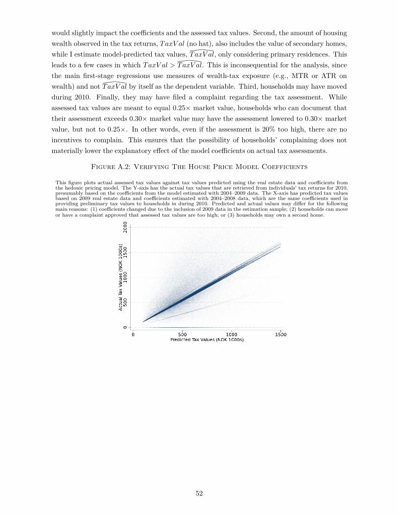
would slightly impact the coefficients and the assessed tax values. Second, the amount of housingwealth observed in the tax returns, TaxV al (no hat), also includes the value of secondary homes,while I estimate model-predicted tax values, TaxV al

∧

, only considering primary residences. Thisleads to a few cases in which TaxV al > TaxV al

∧

. This is inconsequential for the analysis, sincethe main first-stage regressions use measures of wealth-tax exposure (e.g., MTR or ATR onwealth) and not TaxV al∧

by itself as the dependent variable. Third, households may have movedduring 2010. Finally, they may have filed a complaint regarding the tax assessment. Whileassessed tax values are meant to equal 0.25× market value, households who can document thattheir assessment exceeds 0.30× market value may have the assessment lowered to 0.30× marketvalue, but not to 0.25×. In other words, even if the assessment is 20% too high, there are noincentives to complain. This ensures that the possibility of households’ complaining does notmaterially lower the explanatory effect of the model coefficients on actual tax assessments.

Figure A.2: Verifying The House Price Model Coefficients

This figure plots actual assessed tax values against tax values predicted using the real estate data and coefficients fromthe hedonic pricing model. The Y-axis has the actual tax values that are retrieved from individuals’ tax returns for 2010,presumably based on the coefficients from the model estimated with 2004–2009 data. The X-axis has predicted tax valuesbased on 2009 real estate data and coefficients estimated with 2004–2008 data, which are the same coefficients used inproviding preliminary tax values to households in during 2010. Predicted and actual values may differ for the followingmain reasons: (1) coefficients changed due to the inclusion of 2009 data in the estimation sample; (2) households can moveor have a complaint approved that assessed tax values are too high; or (3) households may own a second home.

52

A.4 Descriptive Figures and Tables

Figure A.3: Residential Density Around Borders

This graph shows how residential density varies with border distance. Density is defined at the household level as thelog of the number of households living within 1 km. The figures plot estimated coefficients of living in a given distancebin. The regressions include the baseline housing controls Hi,2009, but these are not allowed to vary at the border-arealevel. Panel A uses distance in kilometers, and Panel B uses scaled distance. All households in the analysis sample (withTaxable Net Wealth ≥ 0 in 2009) are included.

Figure A.4: Geographic Distribution of Households

This figures provides histograms illustrating the distribution of households in the analysis sample according to the differentdistance measures. All households in the analysis sample (with taxable net wealth ≥ 0 in 2009) are included, except thosewith distance measures outside the visible range of the graphs. Panel A uses (signed) distance in kilometers, Panel B usesscaled distance, and Panel C uses relative location, where the green shade indicates membership in the high-assessmentside of the boundary.

53

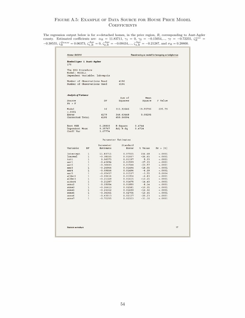
Figure A.5: Example of Data Source for House Price ModelCoefficients

The regression output below is for s=detached homes, in the price region, R, corresponding to Aust-Agdercounty. Estimated coefficients are: αR = 11.83711, γ1 = 0, γ2 = −0.15054,..., γ7 = −0.72255, ζsizeR =−0.38555, ζDenseR = 0.06373, ζAge1,R = 0, ζAge2,R = −0.09434,..., ζAge4,R = −0.21287, and σR = 0.28800.

54

Figure A.6: Example of nonlinearities in a pooled boundaryregion

I employ the following procedure to create this graphical example. First, I create 100 borderareas, indexed by b. Each border area has a length of 200*b, and thus a centroid distancein thousands, e.g., kilometers, (CD) of 100b/1000. Each b has 100 households, equidistantlypopulated in G=[-100b, 100b]. Within each b, house prices move linearly according to theirlocation, g ∈ G: p = ∆

100 . By construction, the mean difference between houses with g < 0(low side) and g > 0 (high side) is constant across bs, and is ∆. I set ∆ to 1. In the first plot,I provide a binscatter of ps against g, separately for b = 10, 25, 50, 75, 100. In the second plot,I perform a pooled binscatter of p, for b ∈ {10, 25, 50, 75, 100}. The red line is a second-orderRD polynomial, estimated separately for each side, allowing for a discontinuity at zero. Pointestimates correspond to the within-bin means for 20 equal-sized bins.

55

Table A.1: Summary Statistics

Summary statistics are provided for households in the sample. Only households who are assigned a signed border distancevariable are included. GFW is Gross Financial Wealth. GFW , censored indicates that GFW is winsorized (censored)at the 95th percentile. TGW is Taxable Gross Wealth. TNW is TGW minus Debt. Labor Earnings (LE) is the sumof wage and salary earnings and max(self employment income, 0). Total Taxable Labor Income (TTLI) is the sum ofLE, UI benefits and other transfers, and labor-related pension income. SMW is the sum of mutual-fund holdings, directholdings of listed domestic stocks and financial securities (excl. deposits) held abroad. TaxV al is the assessed tax value(housing wealth) observed in the tax returns. wtax is the amount of wealth taxes paid. wtax/GFW is set to be themin(wtax/GFW,1). RiskyShare is the ratio of SMW plus non-listed stocks (e.g., private equity) to GFW. Foreign/GFWis the share of GFW that is held abroad. Self -rep/GFW is the share of GFW that belongs to self-reported assetclasses, such as outstanding claims and foreign assets. wtax > 0 is a dummy for whether a household paid wealth taxes.r,Deposits is the realized (symmetric) return on deposits. r,Debt is similarly defined, but excludes households who ineither the current or subsequent period had Debt < 10, 000. Further information on the wealth variables can be found insubsection A.1 in the Appendix.

(A) Main sample (B) Extended sampleUsed in main reduced-form analyses Used for MTR-ATR decomposition

TNW2009 > 0 TNW2009 >-3 MNOK

Obs. weighted by MTC+ATC

N mean sd p25 p50 p75 N mean sd p25 p50 p75GFW, censored 1540156 1000 1109 224 580 1325 2376567 866 953 226 544 11092010–2015, NOK 1000sGFW 1540156 1178 2144 223 580 1324 2376567 964 1721 225 543 1109Debt 1540156 515 1047 0 141 621 2376567 631 1184 0 165 794TGW 1500236 2268 2628 972 1555 2611 2376567 2142 2171 1083 1612 2484TNW 1500236 1743 2409 586 1182 2163 2376567 1512 1979 683 1218 1923T. Taxable L. Income 1543195 694 487 378 581 893 2376567 698 519 355 556 898Labor Earnings 1543195 432 570 0 209 744 2376567 453 601 0 236 753SMW 1540156 153 567 0 0 82 2376567 132 465 0 0 83Domestic Deposits 1540156 722 974 152 407 914 2376567 611 793 145 376 789TaxVal 1506487 833 711 468 664 977 2376567 953 721 554 788 1153wtax 1540258 8 22 0 0 8 2376539 7 17 0 0 7

2004–2009, NOK 1000sTaxVal 1506487 833 711 468 664 977 2376567 953 721 554 788 1153

2010–2015SMW/GFW 1527230 0.108 0.202 0.000 0.000 0.119 2371941 0.119 0.214 0.000 0.000 0.139RiskyShare 1527230 0.164 0.266 0.000 0.006 0.225 2371941 0.169 0.269 0.000 0.009 0.238Deposits/GFW 1527230 0.802 0.292 0.687 0.977 1.000 2371941 0.794 0.296 0.663 0.970 1.000Foreign/GFW 1527230 0.008 0.054 0.000 0.000 0.000 2371941 0.009 0.062 0.000 0.000 0.000Self-rep/GFW 1527230 0.026 0.108 0.000 0.000 0.000 2371941 0.029 0.116 0.000 0.000 0.000wtax/GFW 1521005 0.006 0.033 0.000 0.000 0.007 2371917 0.009 0.048 0.000 0.001 0.008wtax>0 1540258 0.456 0.498 0.000 0.000 1.000 2376539 0.535 0.499 0.000 1.000 1.000

2009r, Deposits (pp.) 1315492 1.94 1.07 1.16 2.03 2.64 2020663 1.94 1.08 1.18 2.01 2.62r, Debt (pp.) 790456 4.04 1.56 3.39 4.07 4.79 1524925 3.94 1.47 3.31 3.96 4.65Age (avg. of adults) 1513409 61.49 13 52 61 70 2291999 61.39 13 52 61 71

56

Table A.2: Summary Statistics When Restricting to Households Near Boundaryand/or Weighting by Propensity to Experience Extensive- Versus

Intensive-Margin Effects

This table provides means for variables during 2010–2015. • Column (1) does not apply any weights or limit the sampleto households near the boundary. Column (2) limits the sample to the 25% of households nearest the boundary in termsof kilometers, by keeping the subsample of households with abs(dkmi ) below the 25th percentile. Column (3) similarlyrestricts the sample to households closest to the boundary in terms of dscaledi . Column (3) weights households by theirMTCi, defined in equation (19), which assigns a higher value to households who would see a greater effect of increasesin TaxV al on their marginal tax rate (MTR) . Column (4) weights households by their ATCi, defined in equation (20).This variable similarly assigns a larger value to households who would see a greater effect on their average tax rate (ATR).Columns (6)-(7) weight by MTC, but consider the 25% subset of households nearest the boundary. Columns (8)-(9) aresimilar to (6)-(7) but instead weight by ATC. • Gross financial wealth (GFW) is the sum of stocks, mutual fund holdings,bonds, and deposits. Taxable net wealth (TNW) equals taxable gross wealth (TGW) minus debt. Stock market wealth(SMW) consists of holdings in listed stocks and mutual funds. TaxVal is assessed housing wealth. T. Taxable L. Incomeis total taxable labor income, which includes labor earnings, as well as pensions and other transfers. Labor earnings is thesum of salary and wage payments and max(self employment income,0). wtax is the amount of wealth taxes accrued in agiven year. Age is measured in 2009. Deposits/GFW is the share of GFW held in deposits (bank savings). Foreign/GFWis the share of GFW held abroad, and not subject to third-party reporting. Self-rep/GFW is the share of GFW that ispotentially self-reported; some subitems may be third-party reported. wtax/GFW is the ratio of wtax to GFW. Int. R.Deposits is the realized average return on deposits. 1[wtax>0] indicates whether a household had to pay any wealth taxes.1[GFW<0,000] indicates whether a household had less than NOK 50,000 in GFW. 1[wtax>0.25*GFW] indicates whethera household accrued wealth taxes in excess of 25% of their GFW.

Weighted – – – MTC ATC MTC MTC ATC ATCNear Boundary – km scaled – – km scaled km scaled

(1) (2) (3) (4) (5) (6) (7) (8) (9)

Panel A: Main Sample 0 < TNW2009 per adult < 6 MNOK

NOK 1000sGFW 1171 1452 1216 757 1352 822 769 1481 1376Debt 510 652 553 467 510 618 516 640 562TGW 2252 2878 2378 1795 2637 2104 1875 3050 2743TNW 1732 2213 1815 1328 2126 1486 1358 2410 2180SMW 150 219 167 93 191 115 99 234 204TaxVal 826 1119 891 842 1026 1059 898 1281 1096Domestic Deposits 719 827 731 528 813 539 526 842 811T. Taxable L. Income 691 784 715 645 703 719 668 778 728Labor Earnings 429 510 451 390 437 462 414 504 460wtax 8 12 9 4 12 5 4 14 12TaxVal2009 532 595 558 537 586 581 562 628 613

Age (avg. of adults) 62 61 61 62 63 62 62 63 63

SMS = SMW/GFW 0.108 0.126 0.113 0.105 0.124 0.117 0.108 0.138 0.129Deposits/GFW 0.803 0.768 0.793 0.823 0.770 0.803 0.817 0.748 0.761Foreign/GFW 0.008 0.012 0.009 0.007 0.011 0.010 0.008 0.014 0.012Self-rep/GFW 0.025 0.035 0.029 0.023 0.034 0.029 0.025 0.041 0.038wtax/GFW 0.006 0.009 0.007 0.007 0.013 0.011 0.008 0.018 0.015TaxVal/TGW 0.478 0.498 0.484 0.535 0.474 0.573 0.545 0.511 0.485Int. R. Deposits (pp.) 1.94 2.05 1.97 1.88 2.13 1.90 1.89 2.15 2.141[wtax>0] 0.453 0.564 0.472 0.456 0.743 0.501 0.462 0.779 0.7481[GFW<50,000] 0.073 0.062 0.073 0.063 0.041 0.068 0.067 0.042 0.0421[wtax>0.25*GFW] 0.002 0.004 0.003 0.004 0.006 0.007 0.005 0.010 0.008

Panel B: Expanded Sample -3 MNOK < TNW2009 per adult < 6 MNOK

NOK 1000sGFW 806 1005 837 726 1287 781 736 1394 1306Debt 1106 1318 1159 627 625 844 694 783 683TGW 1854 2370 1955 1807 2588 2122 1887 2977 2687TNW 733 1034 780 1180 1963 1278 1194 2193 2003SMW 107 156 118 93 184 116 99 223 195TaxVal 827 1098 884 881 1044 1111 940 1297 1112Domestic Deposits 488 565 496 496 770 497 492 787 765T. Taxable L. Income 757 857 780 676 721 763 702 800 747Labor Earnings 564 659 588 439 468 530 467 542 493wtax 5 7 5 3 11 4 4 13 11TaxVal2009 513 563 535 534 582 569 557 619 608

Age (avg. of adults) 55 55 55 61 62 60 60 61 62

SMS = SMW/GFW 0.120 0.137 0.123 0.112 0.128 0.128 0.116 0.143 0.133Deposits/GFW 0.794 0.764 0.788 0.814 0.767 0.789 0.806 0.744 0.758Foreign/GFW 0.007 0.011 0.008 0.008 0.011 0.011 0.009 0.014 0.012Self-rep/GFW 0.027 0.034 0.030 0.025 0.034 0.031 0.027 0.041 0.038wtax/GFW 0.004 0.006 0.004 0.007 0.012 0.010 0.008 0.017 0.014TaxVal/TGW 0.573 0.586 0.577 0.554 0.492 0.594 0.565 0.529 0.503Int. R. Deposits (pp.) 1.72 1.83 1.75 1.84 2.08 1.86 1.85 2.10 2.091[wtax>0] 0.274 0.345 0.285 0.417 0.697 0.446 0.419 0.722 0.6981[GFW<50,000] 0.172 0.145 0.171 0.083 0.055 0.089 0.087 0.057 0.0571[wtax>0.25*GFW] 0.002 0.003 0.002 0.004 0.006 0.006 0.005 0.010 0.007

57

B General Appendix

B.1 Additional figures

Figure B.1: Graphical Presentation of the Reduced-Form Effects onPre-Period Wealth Tax Exposure

These graphs illustrate how geographic discontinuities in tax assessment, TaxV al∧

, affect intensive- and extensive-marginwealth tax exposure during 2004–2009. Panel A considers the effect on the amount of wealth above the threshold andthereby subject to the wealth tax. Panel B considers the extensive-margin effect on whether households are above thethreshold and thereby must face wealth taxation of marginal savings. ◦ The graphs show the reduced-form effect on theseoutcomes of living in a boundary region where households face a 1-log-point tax assessment premium on the high-assessmentside. Circles provide the estimated effect for a given geographic bin. Solid lines provide the linear fit. The discontinuity atzero, jumping from the blue to the green solid line, is the estimated effect of a 1-log point increase in (model-implied) taxassessment, TaxV al∧

. ◦ The first row uses distance in kilometers, where households on the low-assessment side are givena negative distance. The second row uses (similarly signed) distance scaled by the distance between the two municipalcentroids. ◦ Scatter-points stem from estimating a coefficient on ∆i using equation (6) separately for di bins, rather thanestimating coefficients on log(TaxV al

∧

i) and gb(ci)∆i. One negative-distance bin is normalized to be zero. ◦ The sampleincludes households with TNW2009 > 0. The size of each circle corresponds to the relative number of observations in thatbin. Standard errors are clustered at the census-tract level. First-stage effects during 2010–2015 are provided in Table 3 inthe main text.

0-5

0010

0010

0050

0Am

ount

Abo

ve (N

OK

1000

)




-.20

.2.4

1[w

tax

amou

nt>

0]




0-5

0010

0010

0050

0Am

ount

Abo

ve (N

OK

1000

)




-.20

.2.4

1[w

tax

amou

nt>

0]




58

Figure B.2: Household Debt Accumulation Figure, Extensive Version

These graphs consider the effect on household debt accumulation, ∆ log(Debt), during 2004–2009 and 2010–2015 in PanelsA and B, respectively. The first row uses distance in kilometers, where households on the low-assessment side are givena negative distance. The second row uses (similarly signed) distance scaled by the distance between the two municipalcentroids.

-.12

-.08

-.04

0.0

4.0

8.1

2∆l

og(D

ebt)



Panel A: Pre-period

-.12

-.08

-.04

0.0

4.0

8.1

2∆l

og(D

ebt)




-.12

-.08

-.04

0.0

4.0

8.1

2∆l

og(D

ebt)



Panel C: Pre-period

-.12

-.08

-.04

0.0

4.0

8.1

2∆l

og(D

ebt)




Figure B.3: Stock Market Share Figure, Extensive Version

The first row uses distance in kilometers, where households on the low-assessment side are given a negative distance. Thesecond row uses (similarly signed) distance scaled by the distance between the two municipal centroids. ◦ The sampleincludes households with initial TNW > 0.

-.012

-.006

0.0

06.0

12∆S

MS



Panel A: Pre-period

-.012

-.006

0.0

06.0

12∆S

MS




-.012

-.006

0.0

06.0

12∆S

MS



Panel C: Pre-period

-.012

-.006

0.0

06.0

12∆S

MS




59

Figure B.4: Interest Rates on Deposits, Extensive Version

These graphs consider the effect on changes in the realized interest rates on deposits. Panel A considers pre-periodoutcomes (2004–2009) and Panel B considers post-period outcomes (2010–2015). ◦ The graphs below show the reduced-form effect on ∆SMS of living in a boundary region where households face a 1-log-point tax assessment premium onthe high-assessment side. Circles provide the estimated effect for a given geographic bin. Solid lines provide the linearfit. The discontinuity at zero, jumping from the blue to the green solid line, is the estimated effect of a 1-log pointincrease in (model-implied) tax assessment, TaxV al

∧

. ◦ The first row uses distance in kilometers, where households on thelow-assessment side are given a negative distance. The second row uses (similarly signed) distance scaled by the distancebetween the two municipal centroids. ◦ The sample includes households with initial TNW > 0. Scatter-points stem fromestimating a coefficient on ∆i using equation (6) separately for di bins, rather than estimating coefficients on log(TaxV al

∧

i)and gb(ci)∆i. One negative-distance bin is normalized to be zero. The size of each circle corresponds approximately tothe relative number of observations in that bin. Standard errors are clustered at the census-tract level.

-.002

-.001

0.0

01.0

02∆I

nter

est R

ate



Panel A: Pre-period

-.002

-.001

0.0

01.0

02∆I

nter

est R

ate




-.002

-.001

0.0

01.0

02∆I

nter

est R

ate



Panel C: Pre-period-.0

02-.0

010

.001

.002

∆Int

eres

t Rat

e




60

Figure B.5: Pre-Period Version of Labor Earnings Figure

• Figure 6 in the main text provides the estimated effect during the 2010–2015 period.

-.08

-.04

0.0

4.0

8∆l

og(L

abor

Earn

ings

)


Estimated discontinuity: .0093 (SE=.0086)Panel A: Distance in KM

-.08

-.04

0.0

4.0

8∆l

og(L

abor

Earn

ings

)


Estimated discontinuity: .0056 (SE=.0085)Panel B: Scaled Distance Specification

Figure B.6: Extensive-Margin Wealth Tax Exposure for Households with TNWAbove the Wealth Tax Threshold in 2009

This figure illustrates the effect of assessment discontinuities on extensive-margin wealth tax exposure for households initiallyabove the wealth tax threshold (TNW2009 per adult >470,000). This figure otherwise mirrors Panel B.2 of Figure 3.

-.20

.2.4

1[w

tax

amou

nt>

0]



61

Figure B.7: Results on Unadjusted Financial Savings Growth

This figure provides the reduced-form effect on unadjusted financial saving, defined as ∆ log(GFW ). This measure doesnot account for the mechanical wealth-reducing effect of increased wealth tax exposure, and so gives a net-of-wealth-taxsaving measure. The sample and methodology mirrors that of in-text Figure 4, Panel C.

-.1-.0

50

.05

.1∆l

og(G

FW)



Figure B.8: Year-by-Year Boundary Discontinuity Estimates

In this graph, I allow the estimated discontinuities, β, to vary by year. The dashed blue lines provide the main(pooled) estimates. Horizontal lines provide 95% confidence intervals.

-.03

0.0

3.0

6lo

g po

ints

2010 2011 2012 2013 2014 2015

Panel A: Adj. ∆log(GFW)

-.03

0.0

3.0

6lo

g po

ints

2010 2011 2012 2013 2014 2015

Panel B: ∆log(GFW)

-.06

0.0

6.1

2lo

g po

ints

2010 2011 2012 2013 2014 2015

Panel C: ∆log(Debt)

-.01

-.005

0.0

05.0

1fr

actio

n

2010 2011 2012 2013 2014 2015

Panel D: ∆Stock Market Share

-.001

-.000

50

.000

5.0

01in

tere

st ra

te

2010 2011 2012 2013 2014 2015

Panel E: ∆Int. Rate Deposits

-.03

0.0

3.0

6lo

g po

ints

2010 2011 2012 2013 2014 2015

Panel F: ∆log(LaborEarnings)

62

Figure B.9: Simulated Treatment Effects as a Function of the EISwhen incorporating first-stage heterogeneity

This figure shows the how the relationship between simulated treatment effects and the EIS when incorporatingfirst-stage heterogeneity. The sample is split into four quartiles based on TNW2009. First-stage coefficients onMTR and ATRGFW are estimated separately for each group. Table B.12 provides the estimation results andthe subsample-specific summary statistics that underlie this simulation. This contrasts with in-text Figure 7which models the responses of a single shocked agent. High-EIS high-Frisch simulation results are omitted dueto computational (numerical) issues.

-.06

-.03

0.0

3.0

6Δ

log(

GFW

), An

nual

ized

0 .25 .5 .75 1EIS


(A) Financial Savings Growth

-.04

-.02

0.0

2.0

4.0

6.0

8Δ

log(

Labo

rEar

ning

s), A

nnua

lized

0 .25 .5 .75 1EIS


(B) Labor Earnings Growth

63

Table B.1: Subsequent Transaction Outcomes

This table provides the effects of a 1-log-point increase in TaxV al∧

on transaction outcomes during 2010–2016. •Columns (1)-(3) consider log transaction prices, and columns (4)-(6) examine extensive-margin effects, in terms ofa dummy that takes the value 1 if the house the household lived in during 2009 was transacted during 2010–2016.Standard errors are provided in parentheses, and are clustered at the census-tract level. • The geographic slopesin columns (5) and (6) are statistically consistent with the motivating examples discussed in subsection A.2 in theAppendix. These motivating examples would imply coefficients on the scaled border distance variables in column (5)of 1, and a coefficient on the relative location variable in column (6) would of 0.5.

Panel A Panel B

Sale Dummy log(Transaction Price)

(1) (2) (3) (4) (5) (6)

log( TaxV al) 0.0036 0.0021 0.0016 0.2401*** 0.0355 0.0160(0.0029) (0.0028) (0.0023) (0.0835) (0.0853) (0.0721)

1[di < 0] ∗ dKMi ∗∆i 0.0003 0.0504***(0.0004) (0.0152)

1[di > 0] ∗ dKMi ∗∆i -0.0002 0.0414***(0.0004) (0.0152)

1[di < 0] ∗ dscaledi ∗∆i 0.0047 0.9567***(0.0060) (0.1670)

1[di > 0] ∗ dscaledi ∗∆i 0.0044 1.0943***(0.0064) (0.2152)

Relative Locationi * ∆i 0.0031* 0.5922***(0.0018) (0.0596)

N 1540201 1553575 1740546 45422 44667 50203R2 0.1972 0.1931 0.1942 0.5336 0.5380 0.5256

Household controls Yes Yes Yes Yes Yes YesHousing controls (Border spec.) Yes Yes Yes Yes Yes YesGeo-Controls

– Scaled Border Distance Yes – – Yes – –– KM Border Distance – Yes – – Yes –– Relative Location – – Yes – – Yes

B.2 Additional Results Tables

Table B.2: First-Stage Effects on Wealth Tax Outcomes: Using Distance inKM

This table provides the reduced-form estimates that uses border distance in km (as opposed to scaled border distance)as the geographic measure. The sample and methodology is otherwise identical to in-text Table 1 that uses the scaleddistance specification.

Extensive margin Extensive and intensive margin

log(TaxV al) 1[TNW > Threshold] rmarginal AmountAbove raverage

(1) (2) (3) (4) (5)

log( TaxV al) 0.8727*** 0.2406*** 0.2556*** 859122.4803*** 0.2556***(0.0303) (0.0137) (0.0144) (90043.0316) (0.0144)

[1462961] [1426446] [1426446] [1426446] [1426446]F(β = 0) 830 308 316 91 316

Border Distance Controls– KM Yes Yes Yes Yes Yes

64

Table B.3: Main Reduced-form Estimates with Triangular Weights

This table provides regression results when the main IV regression specifications are run with triangular weights. Forthe case of scaled border distance, dscaledi ∈ [−0.6, 0.6], weights are assigned as 1-abs(dscaledi /0.6). For the relativelocation measure, RLi ∈ [−1, 1], weights are assigned as 1-abs(RLi).

adj. ∆ log(GFW ) ∆ log(Debt) ∆SMS ∆Int. R. Deposits ∆ log(L. Earnings)

(1) (2) (3) (4) (5)

Panel A: Scaled Border Distance

log( TaxV al) 0.0182** 0.0025 0.0000 -0.0000 0.0209**(0.0082) (0.0123) (0.0013) (0.0001) (0.0103)

N 1442739 1442756 1437504 1240649 1444211

Panel A: KM Border Distance

log( TaxV al) 0.0143* 0.0080 -0.0005 -0.0001 0.0295***(0.0079) (0.0128) (0.0014) (0.0001) (0.0102)

N 1392561 1392579 1387513 1199969 1393962

Panel A: Relative Location Measure

log( TaxV al) 0.0168** -0.0053 -0.0001 -0.0000 0.0189**(0.0068) (0.0107) (0.0011) (0.0001) (0.0083)

N 1614851 1614871 1608987 1389962 1616524

Table B.4: Robustness: Significance and Standard Errors of MainReduced-form Results using Different Levels of Clustering

Table reports estimated standard errors on log(TaxV al∧

) using different levels of clustering. All regressions are reduced-form, and consider post-period (2010–2015) outcomes. Slightly different point-estimates may occur when clustering at thehousehold or municipality level rather than the census-tract level, as a small number of households are not assigned censustracts.

adj. ∆ log(GFW ) ∆ log(Debt) ∆SMS ∆Int. R. Deposits ∆ log(L. Earnings)

(1) (2) (3) (4) (5)


Household 0.0161** 0.0019 -0.0001 -0.0001 0.0191**(0.0076) (0.0114) (0.0012) (0.0001) (0.0092)

Census tract 0.0163** 0.0025 -0.0001 -0.0001 0.0192**(0.0073) (0.0112) (0.0012) (0.0001) (0.0096)

Municipality 0.0161** 0.0019 -0.0001 -0.0001 0.0191*(0.0072) (0.0101) (0.0013) (0.0001) (0.0107)

Panel A: KM Border Distance

Household 0.0163** 0.0058 -0.0005 -0.0001 0.0331***(0.0075) (0.0115) (0.0012) (0.0001) (0.0091)

Census tract 0.0163** 0.0062 -0.0005 -0.0001 0.0328***(0.0073) (0.0113) (0.0012) (0.0001) (0.0094)

Municipality 0.0163** 0.0058 -0.0005 -0.0001 0.0331***(0.0071) (0.0118) (0.0012) (0.0001) (0.0096)

Panel A: Relative Location Measure

Household 0.0147** -0.0049 -0.0000 -0.0001 0.0209***(0.0063) (0.0094) (0.0010) (0.0001) (0.0076)

Census tract 0.0146** -0.0048 -0.0000 -0.0001 0.0209***(0.0063) (0.0094) (0.0010) (0.0001) (0.0078)

Municipality 0.0147** -0.0049 -0.0000 -0.0001 0.0209***(0.0058) (0.0092) (0.0011) (0.0001) (0.0075)

65

Table B.5: Main results under different geographic bandwidth choices

This table shows the results from the main regressions using different bandwidths (geographic cutoffs). Panel Aconsiders the scaled distance measure. bw=0.9 implies retaining all households with a scaled border distance inside[-0.9,0.9]. The main specification uses bw=0.6. Panel B considers border distance in kilometers (KM). bw=10 impliesretaining all households with a border distance, in km, inside [-10,10]. The main specification uses bw=10. PanelC considers the relative location measure. bw = 0.6 implies retaining all households where their differential distanceto the centroid of the high (versus low) side of the boundary is smaller than 0.6 times the distance between the twocentroids. The main specification uses bw = 1.0.

adj. ∆ log(GFW ) ∆ log(Debt) ∆SMS ∆Int. R. Deposits ∆ log(L. Earnings)Bandwidth (1) (2) (3) (4) (5)


bw = .9 0.0144** -0.0022 0.0001 -0.0001 0.0264***(0.0065) (0.0099) (0.0010) (0.0001) (0.0085)

bw = .8 0.0147** -0.0008 -0.0001 -0.0001 0.0260***(0.0066) (0.0102) (0.0010) (0.0001) (0.0086)

bw = .7 0.0156** -0.0007 0.0001 -0.0001 0.0263***(0.0068) (0.0105) (0.0011) (0.0001) (0.0090)

bw = .6 0.0163** 0.0025 -0.0001 -0.0001 0.0192**(0.0073) (0.0112) (0.0012) (0.0001) (0.0096)

bw = .5 0.0145* 0.0065 0.0005 -0.0001 0.0228**(0.0081) (0.0125) (0.0013) (0.0001) (0.0103)

bw = .4 0.0170* 0.0067 0.0002 -0.0002 0.0154(0.0095) (0.0143) (0.0015) (0.0001) (0.0118)

bw = .3 0.0260** -0.0027 -0.0006 -0.0000 0.0265*(0.0116) (0.0178) (0.0019) (0.0002) (0.0147)

bw = .2 0.0482*** 0.0028 -0.0013 0.0005** 0.0462**(0.0175) (0.0254) (0.0025) (0.0002) (0.0190)

Panel B: KM Border Distance

bw = 14 0.0183*** 0.0048 0.0007 -0.0002* 0.0314***(0.0063) (0.0098) (0.0011) (0.0001) (0.0083)

bw = 12 0.0172** 0.0073 0.0001 -0.0001 0.0340***(0.0067) (0.0105) (0.0011) (0.0001) (0.0089)

bw = 10 0.0163** 0.0062 -0.0005 -0.0001 0.0328***(0.0073) (0.0113) (0.0012) (0.0001) (0.0094)

bw = 8 0.0184** 0.0114 -0.0002 -0.0001 0.0327***(0.0081) (0.0126) (0.0014) (0.0001) (0.0104)

bw = 6 0.0238*** 0.0047 -0.0007 0.0000 0.0225*(0.0092) (0.0150) (0.0016) (0.0001) (0.0122)

bw = 4 0.0333*** 0.0164 -0.0019 0.0001 0.0239(0.0118) (0.0188) (0.0020) (0.0002) (0.0151)

bw = 2 0.0186 -0.0180 -0.0048 0.0004 0.0492**(0.0195) (0.0315) (0.0032) (0.0003) (0.0240)

bw = 1 -0.0138 0.0325 -0.0120* 0.0009 0.0249(0.0391) (0.0626) (0.0070) (0.0006) (0.0478)

Panel C: Relative Location

bw = 1 0.0146** -0.0048 -0.0000 -0.0001 0.0209***(0.0063) (0.0094) (0.0010) (0.0001) (0.0078)

bw = .9 0.0151** -0.0079 -0.0002 -0.0000 0.0188**(0.0066) (0.0102) (0.0011) (0.0001) (0.0083)

bw = .8 0.0148** -0.0030 0.0003 -0.0001 0.0171**(0.0070) (0.0110) (0.0011) (0.0001) (0.0087)

bw = .7 0.0176** -0.0028 0.0002 -0.0000 0.0147(0.0076) (0.0118) (0.0012) (0.0001) (0.0091)

bw = .6 0.0217*** 0.0038 -0.0009 -0.0001 0.0146(0.0080) (0.0128) (0.0013) (0.0001) (0.0100)

bw = .5 0.0227** -0.0067 -0.0006 -0.0000 0.0234**(0.0092) (0.0141) (0.0014) (0.0001) (0.0106)

bw = .4 0.0219** -0.0143 0.0000 -0.0000 0.0173(0.0107) (0.0158) (0.0016) (0.0001) (0.0123)

bw = .3 0.0247** -0.0292 -0.0001 -0.0001 0.0184(0.0124) (0.0197) (0.0019) (0.0002) (0.0144)

66

Table B.6: Boundary Discontinuity Estimates Under Different Specifications

This table shows the effect of changing tax assessment on financial saving during 2010–2015. log(TaxV al) is instru-mented with the model-implied variation in tax assessment. Column (1) does not address geographic heterogeneity,and does not allow slopes on housing characteristics, Hi, to vary at the border-area level. Column (2) allows slopesto vary at the border-area level, but does not address within-border area geographic heterogeneity. Columns (3)-(5)address geographic heterogeneity according to the main specification in equation (6). Column (4) corresponds to thepreferred (scaled) border distance measure. Census-tract-level clustered standard errors are in parentheses. Samplesize is in brackets. F is the Kleinbergen-Paap rk-F statistic of the first-stage regression. One, two, and three starsindicate that estimates are statistically different from zero at the 10, 5, and 1 percent level, respectively.

(1) (2) (3) (4) (5)

No geo. Boundary FEs KM Distance Scaled Distance Rel. Location

∆ log(Gross Financial Wealth), adjusted for wealth-tax payments

log( TaxV al) 0.0183*** 0.0181*** 0.0164** 0.0161** 0.0147**(0.0010) (0.0031) (0.0073) (0.0073) (0.0063)

N 1802589 1802494 1426960 1442739 1614965

∆ log(Debt)

log( TaxV al) 0.0266*** 0.0217*** 0.0057 0.0019 -0.0049(0.0015) (0.0048) (0.0113) (0.0112) (0.0094)

N 1802610 1802515 1426978 1442756 1614985

∆Interest Rate on Deposits

log( TaxV al) -0.000142*** -0.000030 -0.000118 -0.000075 -0.000099(0.000014) (0.000047) (0.000106) (0.000104) (0.000086)

N 1552870 1552772 1230322 1240649 1390060

∆Stock Market Share

log( TaxV al) 0.000291* 0.000238 -0.000521 -0.000119 -0.000040(0.000169) (0.000492) (0.001217) (0.001181) (0.000974)

N 1796010 1795917 1421759 1437504 1609101

∆log(LaborEarnings)

log( TaxV al) 0.0144*** 0.0135*** 0.0329*** 0.0191** 0.0209***(0.0012) (0.0041) (0.0095) (0.0096) (0.0078)

N 1804474 1804378 1428407 1444211 1616639

Controls

Household Characteristics Yes Yes Yes Yes YesHousing Characteristics Yes Yes Yes Yes Yes– Border specific – Yes Yes Yes Yes

Border Distance Controls– KM – – Yes – –– Scaled – – – Yes –Relative Location Controls – – – – Yes

B.3 Effect on municipal finances

Households in high-taxation municipalities may see the negative income effect partially offsetby a higher provision of public goods or a lowering of municipal fees. While this may generallybe a cause for concern, I argue that this effect is likely negligible in my empirical setting forthe following key reasons: First, wealth taxes are disproportionately paid by the very wealthy,who were not disproportionately affected by this reform given that housing wealth accounts

67

for a very small fraction of net worth for the very wealthy (see Fagereng, Guiso, Malacrino,and Pistaferri (2020)). Thus, changes in tax assessments are not likely to lead to meaningfulchanges in the aggregate amount of wealth tax revenues in a given municipality. In addition,wealth taxes account for only 10% of aggregate municipal tax revenues, and drops to only 4% ofwhen considered relative to aggregate municipal total incomes. Finally, due to the government’srevenue equalization scheme, increasing per capita tax revenues by 1 NOK lowers transfers fromthe central government by 0.6 NOK. Therefore, even if wealth tax revenues do change, the effecton local public services would be likely muted, due to a limited effect on municipality finances.Calculations that I present below, suggest that a municipality where assessed tax values ofhousing are 0.5 log points higher will have 0.26% more revenue.53 Thus any reasonable boundson household sensitivity to municipal finances suggest that the effect will be negligible.

B.4 Property Taxation

In 2015, 242 out 428 municipalities levied property taxes on residential homes.54 Startingin 2015, a subset (49) of municipalities began using the tax authorities’ assessments (TaxV al

∧

)to assess property taxes. Prior to 2014, municipalities were not allowed to access or use theseassessments. In order to allow municipalities to reduce costs by limiting the need to performindependent assessments, the tax authorities allowed municipalities to use their assessmentsas of 2014. Initially, municipalities were discouraged from using the measure, by only beingallowed to assess property taxes based on a downward-adjusted (by 33%) version of TaxV al

∧

,which would limit municipal property tax revenues. This disincentive was partially reduced in2015, when TaxV al∧

only needed to be reduced by 20%. A continuing disincentive is that thetax authorities do not allow muncipalities to use their own information to adjust or fine tuneTaxV al∧

. This may be problematic, as municipalities may want to extract higher taxes fromhouses with better locations within an area (e.g., a view of the ocean or larger property size).Neither of these two factors are accounted for in TaxV al

∧

.

The potential use of TaxV al∧

for property-tax purposes implies some scope for the exclusionrestriction to be violated: Border discontinuities in TaxV al

∧

may affect property taxes for asubset of households as of 2015, thereby amplifying (over-stating) the income effects associatedwith a pure wealth tax treatment. To ensure that this is not driving my results, I performtwo robustness exercises. In Panel A of B.7, I exclude 2015 completely. In Panel B, I omitmunicipality-year observations in which TaxV al

∧

is reported to be used for property taxation53I use the distribution of wealth tax payers from SSB (https://www.ssb.no/statbank/table/08231/tableViewLayout1/),

and assume that this distribution holds for all municipalities. In my empirical setting, a 0.5 log point increasein TaxV al increases the amount subject to a wealth tax by 478,000 for households initially above the wealthtax threshold. This increases wealth tax payments by approximately 5,000. Using the distribution of wealthtaxpayers, I increase everyone’s tax payments by 5,000, and find an increase in total tax payments of 25%.Assume that this occurred in one municipality, but not its neighbor. Since the municipal share of the wealthtax is only 64%, the high-side municipality now has 0.64*0.25=16% more wealth tax revenue. The wealth tax’sshare of tax revenue is 10%. Thus the high-side will have 1.6% more tax revenue, but only 1.6% * 40% =0.64% more total revenue, since tax revenues account for 40% of total incomes on average. Only 40% of thisdifference will pass through after applying the government revenue equalization scheme, leaving only 0.26%more revenue for the high-assessment side municipality.

54Source: Statistikkbanken at Statistics Norway, series 12503: Eiendomskatt (K) 2007–2019. 180 is the numberof municipalities that report collecting strictly positive property taxes on a standard house (Enebolig, 120kvm).

68

purposes. Reassuringly, both Panels A and B yield virtually identical results as those estimatedwith the baseline sample criteria, which are provided in Panel C.

An additional argument against property taxation playing a confounding role is that theestimated effects are not driven by the last years of my sample. This is clear from considering theyear-by-year decomposition of saving and labor earnings responses in Figure B.8: I find similareffects for all years, including the early years where there was no opportunity for municipalitiesto base their property taxes on TaxV al

∧

. While its certainly possible that Norwegian householdsrespond to increased property taxation, this response (in terms of e.g., increased saving) is likelyto occur after my sample ends in 2015, when this subset of households realized they would facehigher future property taxes. Property taxation is also more likely to disproportionately affectlower-TNW households than those providing most of the identifying variation in my setting,namely those near or above the wealth tax threshold. Thus, my finding that the positive savingeffect is driven by ATR effects rather than MTR (which is more significantly affected for lower-TNW households) is inconsistent with property taxation playing a confounding role.

Table B.7: Robustness Exercises Related to Property Taxation

This table provides results for the main sample of households with TNW2009 > 0. Panel A omits observations during2015, and adds a control variable for the municipal property tax rate. This panel clusters standard errors on themunicipality level. Panel B keeps observations during 2015 and, unlike the main baseline sample restriction, it keepsobservations where the households live in municipalities that report using TaxVal for property tax purposes. PanelC provides the main results, using the baseline sample restrictions, as a reference. Panels B and C cluster standarderrors on the census-tract level, as per the main specification.

Adj. ∆ log(GFW ) ∆log(Debt) ∆SMS ∆Int. R. Dep. ∆ log(L. Earnings)

(1) (2) (3) (4) (5)

Panel A: Omit 2015; and control for prop. tax rate

log( TaxV al) 0.0180** 0.0008 0.0002 -0.0001 0.0191(0.0077) (0.0122) (0.0013) (0.0001) (0.0119)

Prop. Tax (%) -0.0061* -0.0009 -0.0009 -0.0001 0.0084***(0.0032) (0.0050) (0.0006) (0.0001) (0.0028)

N [1234147] [1234160] [1230315] [1233282] [1235608]

Panel B: Keep 2015; and obs. where muni uses TaxVal for prop. tax

log( TaxV al) 0.0167** 0.0023 0.0000 -0.0001 0.0190**(0.0073) (0.0111) (0.0012) (0.0001) (0.0095)

N [1473681] [1473698] [1468248] [1242017] [1475153]

Panel C: Main specification for reference

log( TaxV al) 0.0163** 0.0025 -0.0001 -0.0001 0.0192**(0.0073) (0.0112) (0.0012) (0.0001) (0.0096)

N [1444279] [1444296] [1439042] [1241961] [1445751]

Geo-Controls

Scaled Border Distance Yes Yes Yes Yes Yes

69

B.5 MTR-ATR decomposition of portfolio allocation effects

Table B.8: Differential Portfolio Responses to Changing Marginaland Average Tax Rates on Wealth

This table reports IV estimates of the effect of changing the marginal (MTR) and average tax rates (ATR) on portfolioallocation as referred to in subsection 6.2.2 in the main text. Columns (1)-(3) consider the stock market share of financialwealth. Columns (4)-(6) consider the realized interest rate on bank savings. Geographic assessment discontinuities,1[di > 0]∆i, interacted with MTCti and ATCti are used as instruments. MTCti and ATCti are based on 2009 observablesand time t tax rules to provide the simulated impact of tax-assessment increases on MTR and ATR. The estimation samplealso includes households with TNWi,2009 < 0; and all coefficients, on instruments and control variables, are allowed tovary by whether TNWi,2009 > 0. ATR+MTR provides thee sum of the coefficients on MTR and ATR. Standard errorson the sum are calculated using the covariance matrix of the estimated coefficients. Stars indicate significance at the10%, 5%, and 1% levels. Standard errors are clustered at the census-tract level.

(1) (2) (3) (4) (5) (6)

Panel A: ∆SMS Panel B: ∆ Int. Rate on Deposits

MTR -0.10 -0.01 -0.05 -0.10*(0.33) (0.50) (0.03) (0.05)

ATR -0.41 -0.27 -0.05 0.18*(0.87) (1.01) (0.08) (0.10)

ATR+MTR -0.28 0.08s.e. (ATR+MTR) 0.71 0.07

First-stage F -statistic 253.41 150.25 81.04 253.95 152.31 86.71N 2469362 2469362 2469362 2124479 2124479 2124479

Instruments1[di > 0]∆i ×MTCti Yes – Yes Yes – Yes1[di > 0]∆i ×ATCti – Yes Yes – Yes Yes

B.6 Communication of policy change

The implementation of a new methodology to assess housing wealth was primarily commu-nicated in a letter sent to all homeowners in August of 2010. The letter was titled “Informationfor the calculation of new tax values for residential properties,”55 and provided registered infor-mation about the house, namely structure type, construction year and size. Home-owners wereasked to verify and possibly correct this information, either by postal service or online. At thesame time, “tax calculators” were made available online on the tax authorities’ website, wherehouseholds could enter the characteristics of their home and see their estimated new tax value.This tax value differed somewhat from the actual assessed values, since the online calculatorsused pricing coefficients based on 2004–2008 transaction data, while the final assessment for 2010used coefficients based on 2004–2009 data. The fact that a new assessment methodology wasintroduced was therefore salient, and the effect on a household’s wealth tax base (TNW) wasalready available in the early fall of 2010. On December 15 2010, preliminary tax information(“tax cards”) was sent out to all tax payers, containing estimated taxes to be paid for thatyear, which included the new housing assessment and TNW. Households should thus have beenaware of the financial impact of the new assessment methodology before Christmas of 2010 at55My own translation.

70

the latest.

The tax authorities’ website states that tax values are assessed as the size of the home multi-plied with a price-per-square meter coefficient, which is based on Statistics Norway’s real estatetransaction statistics:“Boligens boligverdi er lik boligens areal multiplisert med kvadratmeter-pris basert pastatistikk over omsatte boliger.” (March 2019). See the tax authorities’ website,where no details are provided on the exact methodology.

C Tax Behavior: Tax-base Elasticity and Effect on Self-ReportedWealth

(Referred to in Section 6.2.3 of the main text)

Taxable Net Wealth (TNW). I first study the effect on the wealth-tax base, TNW , incolumns (1)-(3) of Table B.9. I define adjusted log(TNW ) the following way.

Adj. log(TNW ) = log(qt + max(TNWi,t − TaxV ali,t + TaxV ali,2009, 0)), (26)

where qt shifts the log-argument away from zero by an inflation-adjusted NOK 100,000,56 and themechanical effects of the assessment discontinuities are removed by replacing concurrent housingassessments with the initial assessment. This definition removes variation from households withtwo periods of negative TNW , which is reasonable given that these households typically don’tsee a large effect on their wealth-tax exposure.

The main result is in column (3) of Table B.9, where I decompose the response into amarginal and average tax rate effect. To my knowledge, the estimated combined effect of 4.58(se=3.47) is the first direct estimate of an uncompensated wealth tax base elasticity.

How do these estimates compare to the existing literature? Brulhart, Gruber, Krapf, andSchmidheiny (2021) provide a summary of existing estimates in their Appendix Table A.1. Theirown findings indicate 5-year semi-elasticities of -43 and -96. For simplicity, I wrongfully assumethat their variation is fully driven by MTR effects. Since my MTR effects are negative, andthe ATR effects positive, this provides the best hope for producing consistent findings. Bymultiplying the MTR coefficient in column (3) by 5, I obtain a 5-year MTR elasticity of -9.15,with a lower bound on the 95% confidence interval of -22.65. Thus, I can I statistically ruleout that my findings are consistent with their point estimates. This, however, is not surprisinggiven the evidence they provide in favor of substantial evasion responses in their setting. UsingTable A.1 in Brulhart, Gruber, Krapf, and Schmidheiny (2021), we also see that the implied8-year elasticity in Jakobsen, Jakobsen, Kleven, and Zucman (2020) is -17 to -25. Rescaled to5-year elasticities, they are -11 to -16. Thus their findings are statistically comparable to mine,but only to the extent that ATR effects in their setting are very small.57

This comparison illustrates the usefulness of the MTR-ATR decomposition when considering56TNW levels are typically considerably larger than GFW levels, hence the higher log-shifter.57Jakobsen, Jakobsen, Kleven, and Zucman (2020) discuss how marginal tax rates were affected, but not how this

corresponded to changes in average tax rates.

71

the effects on the wealth tax base. Any particular tax reform can, to some extent, be summarizedas a convex combination of a reduction in marginal and average tax rates, which maps directlyinto linear-return and virtual-income decomposition (see Section E in the Appendix).

In sum, my findings here suggest that behavioral responses are not a large concern in asetting with limited evasion opportunities. This is in line with the views on wealth taxationelicited in surveys by Fisman, Gladstone, Kuziemko, and Naidu (2020). Using textual analysesof respondents’ justifications of various wealth tax schemes, they find little evidence of anyexpressed concerns about the tax base being elastic.

Table B.9: Differential Tax Adjustments to Changing Marginaland Average Tax Rates on Wealth

This table reports IV estimates of the effect of changing the marginal (MTR) and average tax rates (ATR) on the wealthtax base, TNW, as well as the self-reported component of GFW. The adjusted log(TNW) is defined in (26). Columns(1)-(3) consider TNW , which is adjusted to remove the mechanical correlation caused by higher TaxV al. This is doneby replacing TaxV ali,t with TaxV ali,2009. Columns (4)-(6) consider the self-reported components of GFW. Geographicassessment discontinuities, 1[di > 0]∆i, interacted with MTCti and ATCti are used as instruments. MTCti and ATCtiare based on 2009 observables and time t tax rules to provide the simulated impact of tax-assessment increases on MTRand ATR. The estimation sample also includes households with TNWi,2009 < 0; and all coefficients, on instruments andcontrol variables, are allowed to vary by whether TNWi,2009 > 0. ATR + MTR provides the sum of the coefficientson MTR and ATR. Standard errors on the sum are calculated using the covariance matrix of the estimated coefficients.Stars indicate significance at the 10%, 5%, and 1% levels. Standard errors are clustered at the census-tract level.

(1) (2) (3) (4) (5) (6)

Panel A: ∆ log(Adj. TNW) Panel B: ∆ log(Self-reported GFW)

MTR -0.47 -1.51 3.51* 5.56*(1.86) (2.73) (1.96) (3.07)

ATR 6.46 5.67 8.38 -8.11(4.32) (5.14) (6.02) (6.97)

ATR+MTR 4.16 -2.55s.e. (ATR+MTR) 3.52 5.01

First-stage F -statistic 252.84 149.70 81.23 253.41 150.10 81.29N 2464590 2464590 2464590 2471819 2471819 2471819

Instruments1[di > 0]∆i ×MTCti Yes – Yes Yes – Yes1[di > 0]∆i ×ATCti – Yes Yes – Yes Yes

Self-reported Wealth. While the economic significance of self-reported financial assetsin my setting is limited,58 I follow the existing literature in providing new country-specificevidence on the potential for evasion behavior. To do this, I zoom in on the largely self-reportedcomponents of financial wealth, such as securities and real-estate held abroad, in columns (4)-(6)of Table B.9. Both columns (4) and (5) suggest a perhaps surprisingly positive effect of wealthtaxation on reported wealth. Interestingly, the decomposition in column (6) shows that thisis driven by extensive-margin MTR variation. This is exactly the opposite of what we foundfor the main saving measure. This may be indicative of households being more vigilant aboutreporting their non-third-party-reported holdings once they reach the threshold, while becoming58The summary statistics in Table A.1 show that self-reported financial assets only account for 2.6% of GFW at

the mean, and 0% for more than three-quarters of the sample.

72

more likely to misreport once the impact on the annual wealth tax bill becomes larger.

Since this effect appears to be driven by extensive-margin exposure to taxes, it is useful toexamine the potential extent of evasion around the tax threshold in using a bunching analysis.Interestingly, this analysis reveals no evidence of an excess mass of of households located at thewealth tax threshold (see analyses in in Section D in the Appendix). This seems consistent withthe non-negative effect that we found in column (6) arising from extensive-margin exposure.My finding of no bunching at the threshold is in stark contrast with previous findings fromDenmark, Sweden, Colombia, and Switzerland.59 The findings of Seim (2017) and Londono-Velez and Avila-Mahecha (2020a) suggest that evasion may be greatly restricted if self-reportingis limited. My findings are consistent with this, suggesting that evasion is addressable by limitingthe extent of self-reporting, as Saez and Zucman (2019) argue. However, these findings comewith the important caveat that evasion primarily occurs among the very wealthiest individualswhom are already considerably to the right of the threshold. Their responses evasion behaviorwould not be picked up my either my bunching analysis or my above analysis in Table B.9.

D Bunching

There is clear evidence of Norwegian households evading and avoiding capital taxation (see,e.g., Alstadsæter and Fjærli 2009, Alstadsæter, Kopczuk, and Telle 2019b). However, the exist-ing empirical evidence shows that this occurs primarily among very wealthy households. In myempirical setting, I obtain most of my identifying variation from households near the wealth taxthreshold, considerably below the top 1% of the wealth distribution. These households primarilyhold assets that are third-party reported, which greatly lowers the potential extent for evasion.Yet, it is useful to confirm this graphically. Traditional wealth-tax threshold bunching analysesinform the behavior of agents near the tax and is thus well suited for this purpose.

While households may not underreport the amount of deposits they hold in domestic banks,they may, for example, be induced by wealth taxation to shift savings into harder-to-tax assetclasses, such as art. This would imply that my saving measure, based on changes in largelythird-party reported financial wealth, would understate the true effect on saving. I shed somelight on this question following the approach in Seim (2017).

I show my results in Figure B.10 below. Panel A shows the results for my full analysissample, and Panel B shows results for the full sample of Norwegian taxpayers. We see thatthe wealth tax threshold is located at a fairly dense place in the wealth distribution. In PanelA, each NOK 5,000 bin (≈ USD 833, using the 2010 USD/NOK exchange rate of around 6.)contains about 625 households on average in a given year (2500/4 years).

The visual evidence is quite clear, in that there is no sizable bunching around the wealth taxthreshold in either sample. I perform more formal bunching analyses using the the approachof Chetty, Friedman, Olsen, and Pistaferri (2011). Panel B estimates a statistically significantexcess mass around the threshold, but the visual evidence is not very supportive. In Panel B,59See Jakobsen et al. (2020); Seim (2017); Londono-Velez and Avila-Mahecha (2020a); and Brulhart et al. (2019),

respectively.

73

the excess mass, b, equals 0.097, which means that there is 9.7% extra mass in the NOK 5,000bin to the left of the kink. This number is calculated using the methodology of Chetty et al.(2011), and the assumptions closely resemble those made by Seim (2017). First, a counterfactualdistribution is calculated by fitting a 7th order polynomial to all points bins outside [−40k, 15k].Then the relative number of bunchers, N(%), is calculated as the relative difference between thenumber of agents in the empirical and counterfactual distributions within [−40k, 15k]. Then allof the bunchers are assumed to be bunching one bin to the left of the threshold. MultiplyingN(%) by the number of NOK 5,000 bins in [−40k, 15k] then yields b.

Multiplying b by NOK 5,000 tells us that 5, 000b less TNW is being reported due to the wealthtax threshold. In relative terms, given an average threshold during this period of NOK 830,000,and b = 0.097, this implies that 0.05843% of TNW is being misreported. Since the average wealthtax rate during this sample period (2011–2014) was 1.075%, this yields a net-of-tax rate elasticityof taxable wealth (following the definition in Seim (2017)) of 0.05853%/(0.01075/(1−0.01075)) =0.054. When translated to an elasticity with respect to a net-of-tax rate of return of 2%, theelasticity becomes 0.05853%/(0.01075/(2%)) = 0.0010.

Figure B.10: Distribution of Households around the Wealth Tax Threshold

These figures show the distribution of taxable net wealth around the wealth tax threshold. Households are dividedinto NOK 5,000 bins, and households at zero have [0, 5000) NOK in excess of the threshold. Panel A considers thefull analysis sample, where thresholds are multiplied by two for married couples, and only couples with a non-changedmarital status are included. Panel B considers the full sample of Norwegian taxpayers, where the analysis is done atthe individual level. Plots and estimates are produced using the .ado file provided by Chetty, Friedman, Olsen, andPistaferri (2011). The counterfactual distribution (green line) is constructed by fitting a 7th degree polynomial onall bins outside [-40,000, 15,000]. b is the estimated excess mass inside [-40,000, 15,000], normalized to be in the bindirectly to the left of the threshold. Bootstrapped standard errors are in parenthesis. The analyses use pooled datafor 2011–2014. The sample period is restricted due to limited sample years in which the relevant net wealth variable,nto form, is not bottom-coded at the level of the tax threshold.

These findings point toward limited avoidance or evasion behavior in my sample, which isconsistent with evasion or avoidance responses being unlikely to lead my estimated effects onfinancial saving to greatly understate the effect on over-all saving behavior. This is in largepart because I am estimating treatment effects among (only) moderately wealthy households.Wealthier households likely have access to more low cost evasion or avoidance technologies,which is consistent with the findings of Alstadsæter, Johannesen, and Zucman (2019a). Oneexample is the ease of placing wealth in foreign financial assets. Alstadsæter, Johannesen, andZucman (2018) find that only 0.03% of households in the bottom 99% of the wealth distribution

74

(covering almost my entire sample) reported foreign wealth holdings under the protection of atax amnesty. In the top 0.1% of the wealth distribution, on the other hand, a more substantial6% of households reported foreign wealth holdings. While moderately wealthy households maybenefit, in wealth tax sense, by placing assets into harder-to-tax assets such as art, the netbenefit is not clear. Art is considerably less liquid and likely much riskier than financial assetssuch as deposits.

Finally, it is worth noting that little-to-no bunching by itself does not rule out extensiveevasion or avoidance behavior. Such behavior may materialize in ways that is hard to detectby bunching techniques. For example, it may be the very wealthiest who evade and avoid themost, and they might abstain from doing it to the extent where they end up very close to thewealth tax threshold. However, these findings are consistent with the institutional details in mysetting that likely limit such responses for the households that I study.

E Conceptual framework

The purpose of this section is to present a simple two-period life-cycle model of consumptionto relate saving responses to tax-assessment shocks to responses to changes in the net-of-taxrate of return, and show how these responses relate to structural parameters.60 I then show howcomparing the effects of assessment shocks on the marginal versus average net-of-tax rates-of-return can help us assess whether tax assessment shocks can be used as instruments for (linear)rate-of-return shocks.

Consider the following simple two-period model, in which households choose how much toconsume in each period, Ct and may save S in period 1. I focus on saving responses and assumeperfect foresight to keep the model simple. Households have an initial endowment of Y1, whichcan be thought of as initial wealth plus first-period exogenous income, and face exogenous incomeof Y2 in period 2. At the end of this section, I discuss the impact of introducing endogenous laborsupply. The tax authorities impose a tax τ on taxable net wealth, W = SR+A, in excess of athreshold, W . A is some premium the tax authorities add to a household’s wealth, analogousto the empirical variation in tax assessments for the housing component of net wealth.

Baseline optimization problem.

maxC1,C2,S

U(C1, C2, S) = 11− γC

1−γ1 + β

11− γC

1−γ2 , (27)

s.t. C1 + S = Y1 (28)

and C2 = Y2 +RS − τ1[SR+A− W > 0](SR+A− W ). (29)60In the last section, in which I calibrate a life-cycle model to infer which EIS my results can rule out, I use

a multi-period model with endogenous labor supply. However, the key intuition can be found in this simplertwo-period model.

75

We can rewrite the constraint for period 2 as:

C2 = Y2 + SR(1− τ1[SR+A− W > 0]) + τ1[SR+A− W > 0](W −A),

where the last term is virtual income (in period 2), which compensates for the fact that τ isnot applied to all savings due to the tax threshold.

Wealth taxes offer a slightly complicated optimization problem, with agents potentiallybunching such that SR+A−W = 0. Since bunching is not an empirically important phenomenonin my setting, and a few key insights are obtainable with a few simplifying approximations, Itake the following simpler route. First define R = R(1 − τ1[SR + A − W > 0]) and V =τ1[SR + A − W > 0](W − A). We can then rewrite the budget constraint for period 2 asC2 = Y2 + RS + V . Then I assume that agents take R and V as given when they optimize,which can be thought of as a linearization of the budget constraint around the empirical means.The problem then becomes:

Simplified optimization problem.

maxC1,C2,S

U(C1, C2, S) = 11− γC

1−γ1 + β

11− γC

1−γ2 , (30)

s.t. C1 + S = Y1 (31)

and C2 = Y2 + RS + V . (32)

Assuming that constraints bind, imposing the first-order condition on S and reorganizingthen leads to the following expression for S:

S = [βR]1γ Y1

R+ [βR]1γ

− Y2 + V

R+ [βR]1γ

. (33)

Suppose R and V are differentiable with respect to the tax-assessment variable, A. Now Iassume that agents optimally change their behavior when A affects R and V . Their responsecan be decomposed, using the chain rule, as the sum of a rate-of-return effect and a virtualincome effect:

dS

dA= dS

dR

dR

dA︸︷︷︸Rate-of-return Effect

+ dS

dV

dV

dA︸︷︷︸Virtual Income Effect

. (34)

Rate-of-return effect. By reducing the marginal rate-of-return, R, increases in tax as-sessment, A, cause a “traditional” rate-of-return effect, which I write out below.

76

dS

dR= Y1

(1γ− 1

) [βR]1γ

(R+ [βR]1γ )2

+ (Y2 + V )1 + β

γ [βR]1γ−1

(R+ [βR]1γ )2

. (35)

The first term in equation (35) gives rise to the theoretical ambiguity in household responsesto rate-of-return shocks. Its sign depends on the Elasticity of Intertemporal Substitution, 1

γ .The second term is the “human wealth effect”, whereby an increase in R lowers the net presentvalue of future incomes, Y2 + V , which induces more saving.

We can rewrite the expression for dSdR above, using the formula for S, to see the overall

ambiguity more clearly in the presence of a human wealth effect.

dS

dR= 1γ

[βR]1γ

(R+ [βR]1γ )2

(Y1 + Y2 + V

R

)− S

R+ [βR]1γ

. (36)

We see now that if savings are sufficiently positive, S > 0, and the EIS, 1γ , is sufficiently

small, then this expression is negative.61

Virtual Income Effect. By affecting V , shocks to tax assessment cause an additional(virtual) income effect:

dS

dV= − 1

R+ [βR]1γ

. (37)

The magnitude and sign of this channel depends critically on how A affects V . If we definethe average rate of return as Ravg, such that SRavg = SR + V , then we can rewrite V asV = S(Ravg − R), which is simply savings multiplied by the difference between the average andmarginal rates-of-return. We may therefore write the effect of tax-assessment shocks on virtualincome as the following:62

dV

dA= S

(dRavg

dA− dR

dA

). (38)

While these derivatives are not well defined analytically due to the presence of indicatorfunctions, their empirical counterparts can be estimated empirically by considering differential61As an example, consider the case in which βR = 1. Further assume that R = 1.5, and, without loss of generality

(since it will be divided through), that Y2 +V = 1. S > 0 then implies Y1 > 1. In this case, dS/dR ≤ 0 whenever1γ≤ 2.5− 2.5+1/1.5

Y1. Setting Y1 = 1.5, in other words, that current income and wealth exceeds future (nominal)

income and wealth by R− 1 = 50%, yields 1/γ ≤ 0.38.62This assumes that S is not also affected by A in any way that affects V . This is related to the assumption that

agents take R and V as given when choosing the optimal amount of S.

77

effects of tax-assessment shocks on the marginal versus average net-of-tax rates-of-return. Thiswill be a useful exercise, because the differential effects dictate how my tax-assessment shocksyield a treatment comparable to linear rate-of-return shocks.

Relative importance of income and virtual income effects. To understand the rela-tive importance of these two effects, I rewrite the (decomposed) effect of tax assessment shockson saving from equation (34) when the EIS is zero to isolate income effects. I use the expressionfor dS/dR from equation (36), substitute in for dV /dA, and reorganize to get:

dS

dA= − S

R+ 1

(

dR

dA

)︸︷︷︸Income Effect

−(dR

dA− dRavg

dA

)︸︷︷︸Virtual Income Effect

. (39)

The term denoted “Income Effect” represents the effect of tax assessment on saving throughchanging a linear rate-of-return. The second term indicates the effect through changing virtualincome. This equation suggests that we can evaluate the relative impact of these two channels bycomparing the effects of tax-assessment shocks on the marginal versus average rates-of-return.If I find E[dR/dA] to be twice as large as E[dRavg/dA], which suggests that half the incomeeffects are offset by opposing virtual income effects. If I find Ed[R/dA] to be only half that ofE[dRavg/dA], this suggests that income effects are amplified by a factor of two.

Endogenous labor supply. In Section E.1 in the Appendix, I modify the existing opti-mization problem by introducing endogenous labor supply in period 1. The preferences featurea constant Frisch elasticity and additive separability in the (dis)preferences for consumption andlabor supply. This added complexity has no effect on the qualitative conclusions in the previoussection, but shows that the labor earnings response will be of the same sign as, but smaller inmagnitude than, the savings response. The savings response takes the same form, but is scaledup in magnitude. This added responsiveness will depend on the parameters governing laborsupply.

E.1 Two-period model with endogenous labor supply

Consider the modified household optimization problem. L ≥ 0 is hours worked in period 1,W is the exogenous hourly wage, 1

ν > 0 is the Frisch elasticity, and ψ > 0 is the (dis)utility weighton labor supply. Y1, and Y2 are the exogenous incomes in periods 1 and 2, respectively.

maxC1,C2,S,L

U(C1, C2, S, L) = 11− γC

1−γ1 − ψ L

1+ν

1 + ν+ β

11− γC

1−γ2 (40)

s.t. C1 + S = Y1 + LW

and C2 = Y2 + R+ V

78

The first-order conditions with respect to S, together with the budget constraints, implythat:

S = [βR]1γ (Y1 + LW )

R+ [βR]1γ

− Y2 + V

R+ [βR]1γ

. (41)

The first-order conditions with respect to L, together with the budget constraints, implythat:

dL ·W = γ[Y1 + LW − S]−γ−1W 2

(ψνLν−1 + γ[Y1 + LW − S]−γ−1W 2)dS ≡ fdS. (42)

Since ψνLν−1 > 0, and C1 = Y1 +LW −S > 0, this implies that the labor earnings responseis a fraction, f ∈ (0, 1), of the savings response to rate-of-return shocks.

I now totally differentiate equation 41 with respect to R and substitute dL · W for theexpression in equation (42), and solve for dS/dR to get:

dS

dR=

1− f [βR]1γ

R+ [βR]1γ

−1(Y1 + LW )1− γγ

[βR]1γ

(R+ [βR]1γ )2

+ (Y2 + V )1 + β

γ [βR]1γ−1

(R+ [βR]1γ )2

.(43)

I then totally differentiate 41 with respect to V , and substitute dL ·W with the expressionin equation (42), and solve for dS/dV to get:

dS

dV=

1− f [βR]1γ

R+ [βR]1γ

−1− 1R+ [βR]

1γ

. (44)

The expressions for dS/dR and dS/dV are qualitatively similar to the case without endoge-nous labor supply, but are scaled up (in magnitude), since (1 − f [βR]

1γ /(R + [βR]

1γ ))−1 > 1.

The expression for the rate-of-return sensitivity in equation 43 now also contains labor earningsas period 1 income. There is therefore no change in the qualitative conclusions drawn in thecase with only exogenous (labor) income. The new insight is that the effect on labor earningsshould be of a same sign as, but smaller in magnitude than, the effect on savings.

79

Table B.10: Detailed IV Table: Saving Behavior and Labor EarningsResults when not allowing coefficients on instruments to vary by 1[TNWi,2009 > 0]

This table provides results using a slightly simplified version of the regression specification underlying the main results in Table 3. This specification does not allow the first-stage or reduced-formcoefficients on the instruments to covary with 1[TNWi,2009 > 0], which leaves fewer first-stage and reduced-form coefficients to be estimated.

Panel A: IV EstimatesAdj. ∆ log(GFW) ∆ log(GFW), unadj. ∆ log(LaborEarnings)

MTR -0.46 -4.13 -1.84 -4.77 3.13 0.06(1.98) (2.99) (2.02) (3.06) (2.36) (3.49)

ATR 5.70 13.34** 0.62 10.68* 14.75** 11.79(4.43) (5.52) (4.66) (5.73) (6.37) (7.27)

ATR+MTR 9.20 5.91 11.85s.e. (ATR+MTR) 3.63 3.79 5.24

First-stage F -statistic 503.63 297.77 159.51 503.63 297.67 159.48 503.64 297.67 159.48N 2471793 2471793 2471793 2471819 2471819 2471819 2471820 2471820 2471820

Panel B: Reduced-form RegressionsAdj. ∆ log(GFW) ∆ log(GFW), unadj. ∆ log(LaborEarnings)

1[di > 0]∆i *MTCi -0.42 -2.95 -1.70 -3.37 2.89 -0.03(1.82) (2.12) (1.84) (2.14) (2.17) (2.44)

1[di > 0]∆i *ATCi 3.62 6.92** 0.40 4.71* 9.36** 8.24**(2.88) (2.75) (2.96) (2.80) (4.03) (3.80)

N 2471793 2471793 2471793 2471819 2471819 2471819 2471820 2471820 2471820

Panel C: First-stage RegressionsAdj. ∆ log(GFW) ∆ log(GFW), unadj. ∆ log(LaborEarnings)

MTR ATR MTR ATR MTR ATR MTR ATR MTR ATR MTR ATR

1[di > 0]∆i *MTCi 0.92*** 0.69*** -0.01 0.92*** 0.69*** -0.01 2.89 0.69*** -0.01(0.04) (0.04) (0.02) (0.04) (0.04) (0.02) (2.17) (0.04) (0.02)

1[di > 0]∆i *ATCi 0.63*** 0.57*** 0.70*** 0.63*** 0.57*** 0.70*** 9.36** 0.57*** 0.70***(0.04) (0.08) (0.03) (0.04) (0.08) (0.03) (4.03) (0.08) (0.03)

N 2471793 2471793 2471793 2471793 2471819 2471819 2471819 2471819 2471820 2471820 2471820 2471820

80

E.2 Exploring the role of liquidity constraints

To the extent that households in my sample face binding liquidity constraints, the effectsof increased wealth tax exposure may be muted toward zero. Firstly, if substitution effectsdominate, liquidity constrained households cannot dissave further, thus we would not expect tosee considerable dissaving. Secondly, income effects would be muted by the unmet borrowingdemand. We would only observe a positive saving response if income effects were strong enoughto cancel out the unmet borrowing demand and render the household unconstrained.

However, if there is some amount of preference heterogeneity, it becomes possible that liq-uidity constraints disproportionately mute the dissaving responses of high-EIS households. Forthis to have a material effect, a meaningful portion of the households in my sample would haveto face binding liquidity constraints. My descriptive statistics are inconsistent with this. House-holds generally have high levels of liquid wealth, and wealth taxes almost never account for avery large share of GFW.63 While it is unlikely that the small amount of low-GFW householdsare driving my results, I provide a robustness exercise below.

In Table B.11 below, I provide the main MTR-ATR decomposition results when droppinghouseholds with initial GFW below NOK 100,000 (approx. USD 16,667). This leads to a veryliquid sample. Even the 10th percentile of financial wealth is above NOK 125,000 (> USD20,000) during the sample period, which was not guaranteed given that I only conditioned oninitial GFW. When focusing on the households that provide the identifying variation, i.e., thosewith high MTCs and ATCs (defined in Section 6.1), the unconditional 10th percentile is evenhigher. At the means and medians, we see that GFW is above 0.5 MNOK and 1 MNOKrespectively.

The results found in this subsample are qualitatively very similar to those found in Table 3in the main text, and the differences are statistically modest.

To compare the estimates, I scale the differences by the standard errors in Table 3. I findthat MTR effects increase somewhat in magnitude, by about half of a standard error in column(1), and by about one quarter of a standard error in columns (2)-(3). The ATR effects decreasein magnitude for the two saving measures: By around one-third standard error in column (1)and almost half a standard in column (2). For labor earnings, the ATR effect increases by alittle over one-half standard errors.63See Table A.1. Even at the 25th percentile, GFW exceeds NOK 220,000 (USD 36,667). Table A.2 shows that

wealth taxes account for more than 25% of GFW for less than 1% of the sample, including when we limit theattention to households near the boundary, or when we focus on households positioned to experience greaterMTR or ATR effects.

81

Table B.11: IV Table: Saving Behavior and Labor EarningsResults when omitting households with low-moderate initial financial wealth

This table provides results when altering the sample selection underlying the main findings in Table 3 to only includehouseholds with GFW2009 >100,000. The table also provides unconditional sample statistics for GFW.

(1) (2) (3)

Adj. ∆ log(GFW ) ∆ log(GFW ) ∆ log(L. Earnings)

MTR -5.28* -5.45* -1.11(3.18) (3.25) (4.00)

ATR 11.96** 8.71 16.28**(5.58) (5.85) (8.12)

ATR+MTR 6.67 3.26 15.17s.e. (ATR+MTR) 3.70 3.94 5.84

First-stage F -statistic 65.30 65.30 65.29N 1725306 1725324 1725325

Unconditional GFW statisticsunweightedp10 126,852 126,853 126,852p50 556,410 556,410 556,410mean 1,133,516 1,133,513 1,133,513

MTC-weightedp10 152,908 152,908 152,908p50 547,982 547,982 547,982mean 841,928 841,930 841,929

ATC-weightedp10 203,257 203,257 203,257p50 843,101 843,101 843,101mean 1,426,977 1,426,982 1,426,981

82

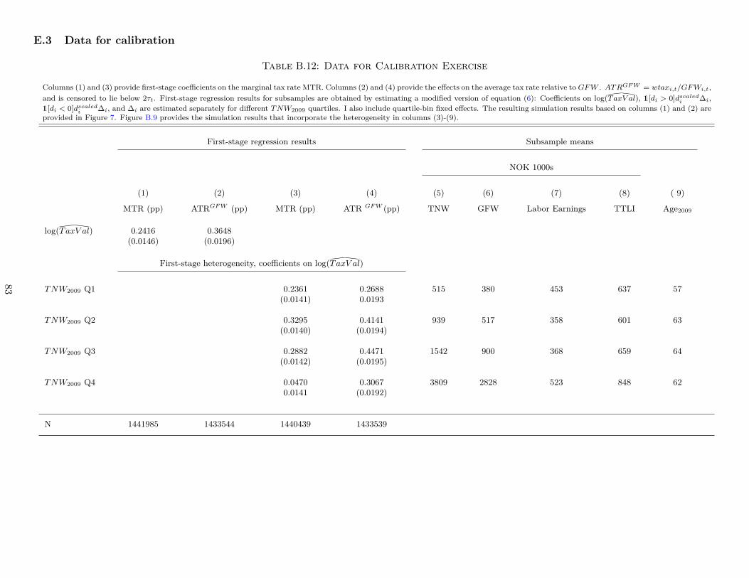
E.3 Data for calibration

Table B.12: Data for Calibration Exercise

Columns (1) and (3) provide first-stage coefficients on the marginal tax rate MTR. Columns (2) and (4) provide the effects on the average tax rate relative toGFW . ATRGFW = wtaxi,t/GFWi,t,and is censored to lie below 2τt. First-stage regression results for subsamples are obtained by estimating a modified version of equation (6): Coefficients on log(TaxV al

∧

), 1[di > 0]dscaledi ∆i,1[di < 0]dscaledi ∆i, and ∆i are estimated separately for different TNW2009 quartiles. I also include quartile-bin fixed effects. The resulting simulation results based on columns (1) and (2) areprovided in Figure 7. Figure B.9 provides the simulation results that incorporate the heterogeneity in columns (3)-(9).

First-stage regression results Subsample means

NOK 1000s

(1) (2) (3) (4) (5) (6) (7) (8) ( 9)

MTR (pp) ATRGFW (pp) MTR (pp) ATR GFW (pp) TNW GFW Labor Earnings TTLI Age2009

log(TaxV al∧

) 0.2416 0.3648(0.0146) (0.0196)

First-stage heterogeneity, coefficients on log(TaxV al∧

)

TNW2009 Q1 0.2361 0.2688 515 380 453 637 57(0.0141) 0.0193

TNW2009 Q2 0.3295 0.4141 939 517 358 601 63(0.0140) (0.0194)

TNW2009 Q3 0.2882 0.4471 1542 900 368 659 64(0.0142) (0.0195)

TNW2009 Q4 0.0470 0.3067 3809 2828 523 848 620.0141 (0.0192)

N 1441985 1433544 1440439 1433539

83

Documents

Wealth Taxation and Household Saving