Weapon System Effectiveness - Unisauir.unisa.ac.za/bitstream/handle/10500/1527/03Chapter3.pdfThe measuring of weapon system effectiveness by using the systems-space reduces to the

-99-

Weapon System Effectiveness 1. APPLICABLE RESEARCH QUESTION In this chapter we address the research question:

If the relationships between a military strategy, its ends, ways and means, are quantified, and if the effectiveness of the force design elements is known, how shall that enable the quantification of the state’s ability to execute its military strategy?

In the first part of this chapter, we shall give an overview of the literature regarding weapon system effectiveness and suggest some improvements to the concept. In the latter part, we shall answer the research question. Finally we shall develop techniques for measuring the underlying components of effectiveness. Recall that we have developed the previous chapter under the assumption that the terminal vertices of M or force design elements are fully combat ready or effective. There is a further implicit assumption that combat readiness and the effectiveness of the force design elements are equivalent concepts. In this chapter, we shall investigate the effects on M when the force design elements are not fully effective. 2. EFFECTIVENESS OF THE FORCE DESIGN ELEMENTS The idea of weapon system effectiveness shall be defined,

• firstly, in general terms;

• secondly, against a state-space background; and

• finally, against a systems-space background. We shall motivate when a systems-space approach is preferable and when a state-space approach might be more applicable. Thereafter, we shall develop a detailed measuring mechanism for weapon system effectiveness based on a systems-space approach to effectiveness.

3

Chapter 3

-100-

2.1. GENERAL NOTIONS REGARDING EFFECTIVENESS The Concise Oxford Dictionary1 defines effectiveness, inter alia,

• as having a definite or desired result;

• to be actually useable;

• to be realisable; and

• fit for work or service. Blanchard and Fabrycky2 define system effectiveness as the probability that a system may successfully meet an overall operational demand within a given time and when operated under specified conditions. In short, system effectiveness is the ability of a system to do a job for which it was intended. Kirkpatrick3 further elucidates this definition when he states that effectiveness depends on the [system’s] success relative to an enemy’s current equipment. For example, Moss4 proposes that, for a fighter aircraft, effectiveness could be the probability that the system would be effective S d i kP P P P= (3.1) where Pd is the probability that the own aircraft will detect the incoming enemy fighter as it comes within attacking range, Pi is the probability that he will intercept the enemy fighter and Pk is the probability that he will kill the enemy aircraft when he fires his weapon. Moreover, Moss holds the position that PS is also a function of own and enemy equipment and personnel effectiveness. However, Blanchard and Fabrycky5 hold that, in themselves, measures such as PS are not sufficient as measures of effectiveness. They hold that system effectiveness is a function of the system’s availability, dependability, performance and other defined measures. We take weapon system performance to be an equivalent concept to weapon system capability or, as in Moss’ example, PS.

1 Concise Oxford Dictionary [The], 9 ed., Oxford, UK: Oxford University Press, 1995, p. 432. 2 Blanchard, B.S. and Fabrycky, W.J., Systems Engineering and Analysis. 2 ed., New Jersey: Prentice Hall, 1990, p. 360. 3 Kirkpatrick, D., Choose Your Weapon: Combined Operational Effectiveness and Investment Appraisal (COEIA) and its role in UK Defence Procurement. London: Royal United Services Institute, 1996, p. 35. 4 Moss, M.A., Applying TQM to Product Design and Development. New York: Marcel Dekker, c1996, pp. 147−148. 5 Blanchard, B.S. and Fabrycky, W.J., op. cit., p. 81.

Weapon System Effectiveness

-101-

2.2. A STATE-SPACE APPROACH TO EFFECTIVENESS The Weapons System Effectiveness Industry Advisory Committee, hereinafter called the WSEIAC, first defined effectiveness during the 1960’s in a state-space environment. By a state-space is meant the state in which a weapon system is, that is, the weapon system is either functioning properly or it is not functioning properly. Thus the WSEIAC nomenclature determines that a system’s state is defined by its condition at a given time. Their work became the established basis for evaluating effectiveness in the US Army6. They define system effectiveness as follows:

Systems Effectiveness7 is a measure of the extent to which a system may be expected to achieve a set of specific mission requirements. It is a function of the system’s availability, dependability and capability.

We now define availability, dependability and capability as follows:

Availability8 is a measure of the system condition at the start of a mission. It is a function of the relationships among hardware, personnel and procedures. Dependability9 is a measure of the system condition at one or more points during the mission, given the system condition at the start of the mission. Capability10 is a measure of the system’s ability to achieve the mission objectives, given the system condition during the mission. Capability specifically accounts for the performance spectrum of the system.

If we consider availability, then, in its simplest form the system, A, may be available or not available. If a system comprises m sub-systems, then the m subsystems may in themselves be available or not available. Note that for m sub-systems, there shall be 2mn = availability combinations. Likewise, for dependability, there shall be n combinations of the state of the system at commencement of a mission, denoted state i, and the state of the system at some later fixed time, denoted state j. Also, there shall exist n capability measures for each case of the n combinations of conditions that the system might be in when called upon to achieve the mission objectives. 6 Engineer Design Handbook - Systems Analysis and Cost-effectiveness, Document AMCP 706-191, Washington: US Army Material Command, 1971, p. 2-18. 7 Ibid. 8 Ibid., p. 2-21. 9 Ibid., p. 2-22. 10Ibid., p. 2-23.

Chapter 3

-102-

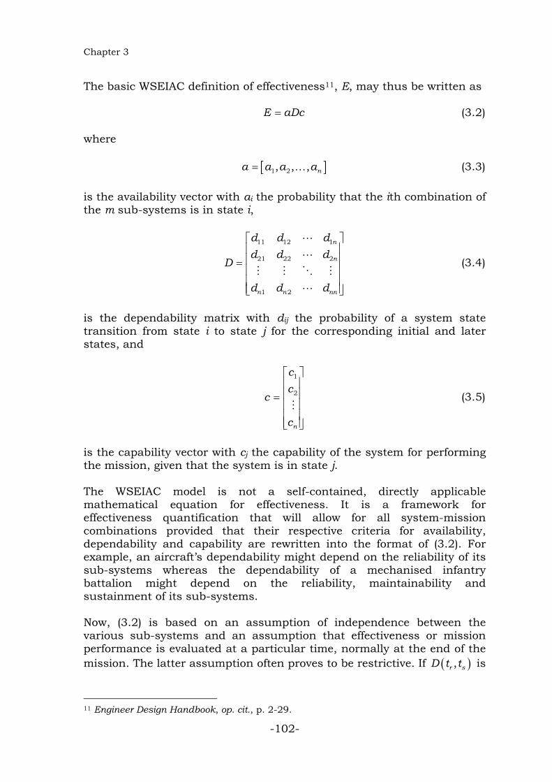
The basic WSEIAC definition of effectiveness11, E, may thus be written as E aDc= (3.2) where [ ]1 2, , , na a a a= … (3.3) is the availability vector with ai the probability that the ith combination of the m sub-systems is in state i,

11 12 1

21 22 2

1 2

n

n

n n nn

d d dd d d

D

d d d

=

(3.4)

is the dependability matrix with dij the probability of a system state transition from state i to state j for the corresponding initial and later states, and

1

2

n

cc

c

c

=

(3.5)

is the capability vector with cj the capability of the system for performing the mission, given that the system is in state j. The WSEIAC model is not a self-contained, directly applicable mathematical equation for effectiveness. It is a framework for effectiveness quantification that will allow for all system-mission combinations provided that their respective criteria for availability, dependability and capability are rewritten into the format of (3.2). For example, an aircraft’s dependability might depend on the reliability of its sub-systems whereas the dependability of a mechanised infantry battalion might depend on the reliability, maintainability and sustainment of its sub-systems. Now, (3.2) is based on an assumption of independence between the various sub-systems and an assumption that effectiveness or mission performance is evaluated at a particular time, normally at the end of the mission. The latter assumption often proves to be restrictive. If ( ),r sD t t is

11 Engineer Design Handbook, op. cit., p. 2-29.


-103-

defined as the dependability matrix over the time interval ( ),r st t and if the Markov assumption holds, that is, ( ) ( ) ( ), , ,r s r i i sD t t D t t D t t= for r i st t t< < , then system effectiveness at time kt is given by ( ) ( ) ( )0,k k kE t aD t c t= . If the mission is one where continuous performance is required over the total mission time, tm, then system effectiveness, assuming well behaved functions, may be quantified as the time-average of ( )kE t 12, that is,

( )0

1 mt

m

E E t dtt

= ∫ .

If the Markov assumption does not hold, then an extension to (3.2) is necessary where c is written as an n × n matrix with an entry for every state transition. 2.3. A SYSTEMS-SPACE APPROACH TO EFFECTIVENESS Now, if we consider the relationship between the m sub-systems and the size, n, of the vectors and matrix in (3.2), we see that 2mn = shall hold. Thus, n shall behave exponentially with m becoming larger. Now suppose a tank regiment comprises of four echelons of thirteen tanks each. To find the effectiveness of the regiment based on the state of the 52 tanks shall necessitate 52 152 4.5 10n = ≈ × entries in the vectors a and c each and n2 entries in D. We conclude by saying that for m large, the analytical application of the WSEIAC framework becomes prohibitive. In order to find a more useable measure for effectiveness we consider the systems-space as opposed to the state-space of the force design element under consideration. To this end, we need to reformulate the definitions of availability, dependability and capability so that they may be applied directly to the weapon system or force design element under consideration. We define Operational Availability, ( )OP A , as the probability that a weapon system is operationally available when called upon to execute a mission. We regard the time of the commencement of the mission to be random event.

12 Engineer Design Handbook, op. cit., p. 2-30.

Chapter 3

-104-

Dependability, ( )OP D A , is the probability that, whilst on a mission, a user system will not suffer a catastrophic failure, that is, the system shall not abort its mission due to some failure. Moreover, we define Capability of a weapon system, ( )OP C D A∩ , to be the probability that a user system is capable of effecting its design for function given it is available and dependable. Recall Blanchard and Fabrycky defined system effectiveness as the probability, ( )P E , that a system may successfully meet an overall operational demand within a given time and when operated under specified conditions. From the above, we have that ( ) ( ) ( ) ( )O O OP E P A P D A P C A D= ∩ . (3.6) By applying Bayes’ rule13 we have that ( ) ( )P E P C= . (3.7) However, we shall observe later that the measuring of the probabilities in the right hand of (3.6) is feasible but the direct measuring of ( )P C poses problems as, on its own, it does not imply the influence of availability and dependability. The measure PS serves as an example. Note that we shall simplify (3.6) to read OE A DC= (3.8) where E, OA , D and C denote ( )P E , ( )OP A , ( )OP D A and ( )OP C D A∩ respectively. We shall use (3.8) in the remainder of the text to define effectiveness. The measuring of weapon system effectiveness by using the systems-space reduces to the product of three scalars as opposed to the billions of entries required by (3.2) for a tank regiment. We shall explain the measuring of AO, D and C in sections 3, 4 and 5. 2.4. A MEASURE OF EFFECTIVENESS An important aspect to take cognisance of in the choice of a measure of effectiveness is the systems level that one is addressing. As we have 13 Steyn, A.G.W., Smit, C.F., Du Toit, S.H.C. and Strasheim, C., Modern Statistics in Practice, Pretoria: J.L. van Schaik, c1994, p. 299.


-105-

indicated, the military strategic means consists of more than one level of abstraction. At the lower end we find the force design elements, often also referred to as user systems. They make up higher order user systems or operating systems. In turn, the operating systems are combined to form systems at the Task Force level or task systems that are charged with the responsibility of achieving the aims related to the military tasks. Furthermore, the example of the tank regiment implies systems at lower levels of abstraction within user systems. The systems directly below user systems in a systems hierarchy are called product systems. The main differentiating characteristics of product systems as opposed to user systems are the following:

• Product systems are purposive systems whereas user systems are purposeful systems. A purposive system is a system that has been designed for some purpose but cannot achieve system objectives or outputs. A purposeful system is a system that can achieve its purpose, objective or output that is was designed for.

• Whereas user systems are systems where main equipment such as ships, tanks and aircraft as well as personnel are integrated by means of doctrine, product systems comprise either main equipment or personnel themselves.

The choice of a suitable measure of effectiveness is between (3.2) and (3.8). We are already aware of the problems associated with (3.2). However, the state-space approach to effectiveness allows for the gradual degradation of effectiveness as more and more sub-systems fail whereas the system-space approach is a single measure at system level and may not readily allow for gradual degradation. If (3.8) can be calibrated to achieve a gradual degradation in the measurement of system effectiveness that is consistent with the effect of the sub-systems starting to fail, then it would be a solution that would allow plausible results that would be sufficiently accurate to allow for fact based decision making. If we consider (3.8) as it relates to user systems, we note that

• OA and D are directly influenced by the maintenance of the product systems that makes up the user systems; and that

• ( )1,..., nC f x x= , where the xi are the capability of the product systems including main equipment and personnel as integrated by applicable doctrine.

Therefore, (3.8) is influenced by logistic and human resource constraints at the product system level in as far as OA and D are concerned and by

Chapter 3

-106-

doctrine at the user system level where C is concerned. Thus, we amend (3.8) to read US

OE A DC= (3.9) where USE denoted the effectiveness of user systems or force design elements. If we follow this argument, then the effectiveness of a higher order user systems or operating system would be ( )1 ,...,OS US US OS

tE f E E I= (3.10) where IOS is the integrator at the operating system level. Likewise, the effectiveness of a task force would be ( )1 ,...,TF OS OS TF

sE f E E I= (3.11) where ITF is the integrator at the task force level. If we analyse (3.10) and (3.11) respectively, we would conclude that the effect of IOS and ITF is a function of command and control doctrine at the operating system and task force levels respectively. Now, we have modelled these entities as force design elements or user systems, so that there exist measures of effectiveness for them of the form (3.9). We may therefore amend (3.10) to read ( )1 ,...,OS US US

tE f E E= (3.12) and (3.11) to read ( )1 ,...,TF OS OS

sE f E E= . (3.13) Consider (3.12). From the previous chapter we have seen that the force design element associated with ijklm contributes ijklmv to the operating

system associated with ijkl ’s enablement. Thus we may write (3.12) comprising of t force design elements as

1

tOS US

mijklmm

E v E=

= ∑ . (3.14)

Also, we may then write (3.13) comprising of s operating systems and where the operating systems contribute ijklv to the enablement of the task force as


-107-

1

sTF OS

lijkll

E v E=

= ∑ . (3.15)

Suppose we prefer (3.10) to (3.12) as the former could be considered more valid than the latter since the integrator OSI affects all force design elements that contributes to the operating system, we may rewrite (3.12) as

1

tOS US OS

mijklmm

E v E I=

= ∑ (3.16)

where the headquarters unit is not included in the summation. It follows that

• finding values for IOS might not be feasible as the capability of the operating system headquarters and its impact on the operating systems might prove to be too complex to determine;

• as (3.14) is a monotone non-decreasing function and it avoids the problem of having to find a value for IOS it will suffice as a measure of effectiveness; and

• we may consider IOS a scaling factor and as we are interested

in relative values only, we may set IOS =1. The argument above also mitigates for (3.15) in favour of (3.11). From the above, we now define measures of effectiveness at the military mission, strategic ends and military strategy levels. Effectiveness of the force design, given r task forces, to execute a military mission is

1

rM TF

kijkk

E v E=

= ∑ , (3.17)

effectiveness of the force design, given q military tasks, to achieve a particular strategic end is

1

qE M

jijj

E v E=

= ∑ , (3.18)

and the effectiveness of the force design, given p military strategic ends, to support a military strategy is

Chapter 3

-108-

1

pR E

iii

E v E=

= ∑ . (3.19)

We note that (3.19) may also be written as

1 1 1 1 1

p q r s tR

ijklm ijklmi j k l m

E v E= = = = =

= ∑∑∑∑∑ (3.20)

where ijklmE relates to the weapon system effectiveness of the force

design element represented at the terminal vertex ijklm of M or as

1

nR

i ii

E w E=

= ∑ (3.21)

where wi is the contribution that the ith force design element makes to the enablement of a military strategy. We shall now consider what the effect shall be of using the actual contribution of a force design element, ijklmρ , to an operating system

instead of the relative contribution, ijklmv , shall be on equation (3.14). Firstly, we may have the situation that

1

1t

USmijklm

mEρ

=

>∑

in which case it is suggested that, in order to comply with the restriction imposed by (2.11) resulting from the relative nature of the vertices where ( ) 5µ ν < , we simply set 1OSEρ = . However, if

1

1t

USmijklm

mEρ

=

≤∑

then we set

1

tOS US

mijklmm

E Eρ ρ=

= ∑ . (3.22)

By setting OS OSE Eρ= then, in turn, it will influence (3.15), (3.17), (3.18) and (3.19) in that they will represent a more accurate representation of the real-world situation.


-109-

2.5. DEPENDENCE BETWEEN FORCE DESIGN ELEMENTS Recall that the relative importance of force design elements regarding their contribution to their applicable operating systems are contained in the relation (2.3). However, in order to find ijklmv we have assumed that the effectiveness of the force design element is equal to one. Furthermore, we have defined the total contribution of a particular force design element to a military strategy by (2.10). Moreover, in this chapter we have indicated that the real contribution that a force design element makes to a military strategy is

1

nR

i ii

E w E=

= ∑ .

Likewise, the real contribution that a force design element makes to an operating system is

1

tOS US

mijklmm

E v E=

= ∑ .

However, it may happen that the effectiveness of a force design element not only depends on its own inherent effectiveness but also on the effectiveness of some other force design element. In this section we develop the following measures for effectiveness:

• The ith Force Design Element is dependent on one or more other Force Design Elements.

• Dependence Trees. • Interdependence.

2.5.1. The ith Force Design Element is dependent on one or more

other Force Design Elements Consider the ith force design element complete with its associated effectiveness iE that was determined by finding availability, dependability and capability for that force design element. Also, suppose there are n force design elements in the force design. It is possible that the ith force design element is dependent on all or some of the other force design elements for it to be able to function properly. It follows that the ith force design element’s effectiveness will be impacted on in proportion to the impact that the effectiveness of the force design

Chapter 3

-110-

elements on which the ith force design element depends shall have on its effectiveness. Thus we have that TDEP

i iE E ep= (3.23) where the effectiveness vector

[ ]1 2 1 1, , , ,1, , ,i i ne E E E E E− += … … ,

the proportion vector

1 2 1 11

, , , , 1 , , ,n

i j i njj i

p p p p p p p− +=≠

= −

∑… …

and where jp is the proportion that the jth force design element’s effectiveness will impact on the effectiveness of the ith force design element. Also note that

0 1jp≤ ≤ and

1

0 1n

jjj i

p=≠

≤ ≤∑ .

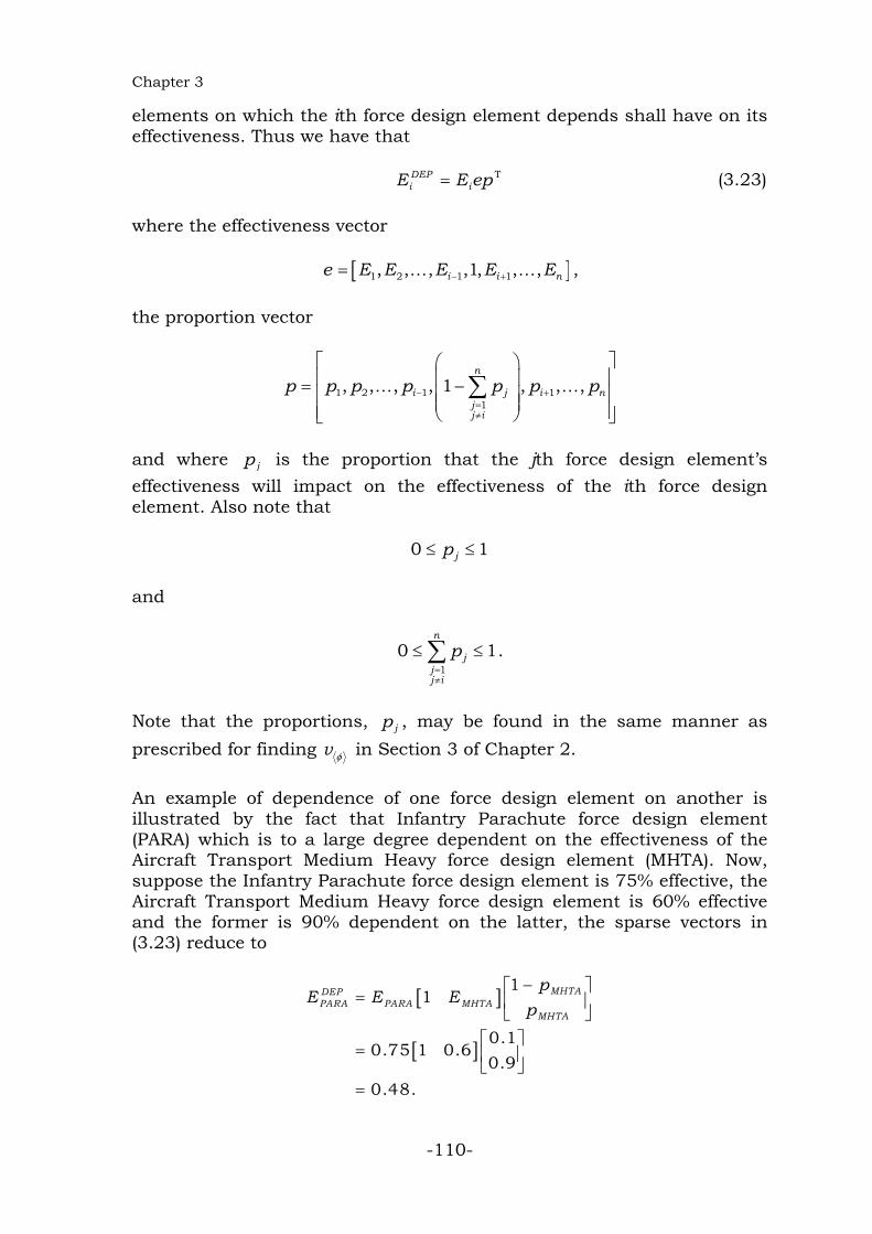
Note that the proportions, jp , may be found in the same manner as prescribed for finding v φ in Section 3 of Chapter 2. An example of dependence of one force design element on another is illustrated by the fact that Infantry Parachute force design element (PARA) which is to a large degree dependent on the effectiveness of the Aircraft Transport Medium Heavy force design element (MHTA). Now, suppose the Infantry Parachute force design element is 75% effective, the Aircraft Transport Medium Heavy force design element is 60% effective and the former is 90% dependent on the latter, the sparse vectors in (3.23) reduce to

[ ]

[ ]

11

0.10.75 1 0.6

0.90.48.

MHTADEPPARA PARA MHTA

MHTA

pE E E

p−

=

=

=


-111-

To prevent self-referencing and its associated problems, on completion we use the adjusted value DEP

iE in lieu of USiE in (3.14) et cetera.

2.5.2. Dependence Trees If the ith force design element’s effectiveness is dependent on jth force design element’s effectiveness, we denote it by i jE E← . Suppose the ith force design element’s effectiveness is dependent on the jth force design element and, in turn, the jth force design element’s effectiveness is dependent on the kth force design element, then we have three force design element’s effectiveness that form a dependence tree. We denote this simple form of a dependence tree as i j kE E E← ← . Likewise, we may find that a dependence tree might, in some places, include force design element’s effectiveness that are dependent on more than one other force design elements’ effectiveness. Now,

j l

mi

k n p

o

E E

EE

E E EE

←

← ← ←

(3.24)

denotes a dependence tree where

• i jE E← and i kE E← ;

• j lE E← ;

• k mE E← , k nE E← and k oE E← ; and

• n pE E← . We solve (3.24) by a recursive algorithm using a depth-first search and employing (3.23) to solve for the various E. The algorithm stops when iE is set to DEP

iE . For example, suppose we have a marine battalion (MAR) that specialises in raids. In turn, the battalion may be transported by sea or air or it may transport itself to the raid area. If it is transported by sea, its effectiveness is dependent on the effectiveness of a landing company (LCY) and if it is transported by air, its effectiveness is dependent on the effectiveness of a transport aircraft (ACT). When travelling overland, it is

Chapter 3

-112-

dependent on its own effectiveness as it transports itself. In turn, the landing company’s effectiveness is dependent on the effectiveness of the personnel landing ship (LSP). We depict this situation in the dependence tree

LCY LSPMAR

ACT

E EE

E←

←

.

2.5.3. Interdependence By interdependence we mean that a set of two or more force design elements’ effectiveness depends on the effectiveness of all the other force design elements in the set. Suppose we have a set of n force design elements that are interdependent. We store their individual effectiveness measurements in the vector [ ]1 2, , , nE E Eε = … and the proportions relating to the interdependence in the n × n matrix

1 12 11

21 2 22

1 2

1

1

1

j nj

j nj

n n njj n

p p p

p p pP

p p p

≠

≠

≠

− − = −

∑

∑

∑

,

where all summations are over n with the restrictions as indicated. To calculate the ith force design elements effectiveness based on its dependency on the others, set e ε= , then set 1ie = and set p equal to the ith row in P, then construct and solve DEP

iE by using (3.23). For example, suppose a frigate (FSG) has a maritime helicopter (MH) and an unmanned aerial vehicle (UAV) onboard. The helicopter and the unmanned aerial vehicle effectiveness is fully dependent on the effectiveness of the frigate whilst the frigate’s effectiveness is 10% dependent on the UAV and 25% dependent on the maritime helicopter. The maritime helicopter and the unmanned aerial vehicle are not dependent on one another. The individual measurements of effectiveness of the three force design elements is as follows:

• FSGE : 0.7. • MHE : 0.8. • UAVE : 0.6.


-113-

We have that [ ]0.7 0.8 0.6ε = and

0.65 0.25 0.1

1 0 01 0 0

P =

.

In the case of the frigate, we construct (3.23) as

[ ]0.65

0.7 1 0.8 0.6 0.250.1

0.637.

DEPFSGE

=

=

For the maritime helicopter, we construct (3.23) as

[ ]1

0.8 0.7 1 0.6 00

0.56.

DEPMHE

=

=

For the unmanned aerial vehicle, we construct and solve (3.23) in the same manner. 2.5.4. Dependence and Interdependence in the South African Force

Design

Force Structure Element Dependent On Degree Dependent On Degree Serial

a b c d e Aircraft Transport Medium Heavy 0.6

1 Infantry Parachute Aircraft Transport

Medium Light 0.2

Helicopter Attack Maritime 0.25

2 Frigate Small Guided Missile Unmanned Aerial

Vehicle Maritime 0.1

3 Helicopter Attack Maritime

Frigate Small Guided Missile 1.0

4 Unmanned Aerial Vehicle Maritime



Special Forces Sea 0.25 Fast Attack Craft Missile 0.75

Aircraft Transport Medium Heavy 0.35

5 Special Forces Land

Aircraft Transport Medium Light 0.1

Table 3.1: Dependencies and Interdependencies

Chapter 3

-114-

An analysis of the operating systems and their associated force design elements in Appendix A revealed dependencies and interdependencies of the effectiveness of force design elements. A short list is contained in Table 3.1 whilst a detailed list is contained in Appendix D. Note that these dependencies and interdependencies, complete with the associated degrees of dependency and interdependency do not constitute the official view of the SANDF, but are based on our subjective judgement and are given as an illustration of the concept. 2.6. REQUISITE CRITERION FOR THE MODEL In order to decide whether (3.8) is a requisite measure of effectiveness, we need to ensure that effectiveness is a function of availability, dependability and capability only14. Recall that Blanchard and Fabrycky hold that system effectiveness is a function of the system’s availability, dependability, performance and other defined measures. They state that satisfactory performance is to be measured by a combination of qualitative and quantitative factors defining the functions that the system or product is to accomplish15. This definition is in essence no different from the definition of capability that defines capability to be a measure of the system’s ability to achieve the mission objectives. As a result, we view performance as an equivalent concept to effectiveness.

Factor Contained in (3.8) Incorporated in Serial

a b c 1 Ability to man Yes Capability 2 Failure rate Yes Availability 3 Maintainability Yes Availability and

Dependability 4 Maintenance down time Yes Availability 5 Mean time between failures Yes Availability

6 Mean time between maintenance

Yes Availability

7 Mean time to repair Yes Availability 8 Operator skills level Yes Capability 9 Personnel efficiency Yes Capability 10 Reliability Yes Dependability

11 Supportability Yes Availability and Dependability

Table 3.2: Factors affecting equation (3.8)

14 Phillips, L.D., Requisite Decision Modelling, Journal of the Operations Research Society, Vol 33, 1982, p. 37. 15Blanchard, B.S. and Fabrycky, W.J., op. cit., p. 347.


-115-

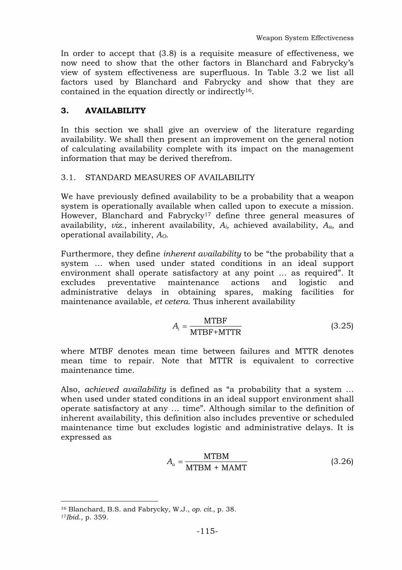
In order to accept that (3.8) is a requisite measure of effectiveness, we now need to show that the other factors in Blanchard and Fabrycky’s view of system effectiveness are superfluous. In Table 3.2 we list all factors used by Blanchard and Fabrycky and show that they are contained in the equation directly or indirectly16. 3. AVAILABILITY In this section we shall give an overview of the literature regarding availability. We shall then present an improvement on the general notion of calculating availability complete with its impact on the management information that may be derived therefrom. 3.1. STANDARD MEASURES OF AVAILABILITY We have previously defined availability to be a probability that a weapon system is operationally available when called upon to execute a mission. However, Blanchard and Fabrycky17 define three general measures of availability, viz., inherent availability, Ai, achieved availability, Aa, and operational availability, AO. Furthermore, they define inherent availability to be “the probability that a system … when used under stated conditions in an ideal support environment shall operate satisfactory at any point … as required”. It excludes preventative maintenance actions and logistic and administrative delays in obtaining spares, making facilities for maintenance available, et cetera. Thus inherent availability

MTBFMTBF+MTTRiA = (3.25)

where MTBF denotes mean time between failures and MTTR denotes mean time to repair. Note that MTTR is equivalent to corrective maintenance time. Also, achieved availability is defined as “a probability that a system … when used under stated conditions in an ideal support environment shall operate satisfactory at any … time”. Although similar to the definition of inherent availability, this definition also includes preventive or scheduled maintenance time but excludes logistic and administrative delays. It is expressed as

MTBMMTBM + MAMTaA = (3.26)

16 Blanchard, B.S. and Fabrycky, W.J., op. cit., p. 38. 17Ibid., p. 359.

Chapter 3

-116-

where MTBM denotes mean time between maintenance and MAMT denotes mean active maintenance time. Both these measures are functions of corrective and preventive maintenance. Lastly, operational availability is “a probability that a system … when used under stated conditions in an actual operational environment shall operate satisfactory when called upon”. It is expressed as

MTBMMTBM + MDTOA = (3.27)

where MDT denotes mean maintenance down time and includes corrective and preventive maintenance as well as logistic and administrative delay time. Note that (3.25), (3.26) and (3.27) are not requisite as they indirectly imply that corrective maintenance time, preventive maintenance time and logistic and administrative delay time are mutually exclusive. For example, 1 iA− would imply corrective maintenance time only whereas

i aA A− would imply preventive maintenance only and as a result no measure exists when both preventive and corrective maintenance could take place simultaneously. We maintain that these concepts are not mutually exclusive, that is, these actions may take place at the same time. Furthermore, as we are interested in force design elements where people are inherent to the system, the non-availability of the system with respect to people should be included in the measures for availability. From a technical perspective, to determine Ai, Aa and AO deterministically may prove difficult, as, for example, complete records for when failures in machinery and human resources occur must be kept. From practical experience, this requirement cannot be met readily. 3.2. MEASURES OF OPERATIONAL AVAILABILITY AND RELATED

COSTS THERETO We have developed the measure so that

• both logistic and human resource events be modelled to find values for the measures of availability;

• the various events be considered not to be mutually exclusive; and

• a stochastic process be used to determine values for the measures of availability.


-117-

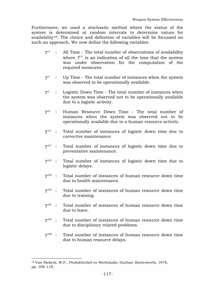
Furthermore, we used a stochastic method where the status of the system is determined at random intervals to determine values for availability18. The choice and definition of variables will be focussed on such an approach. We now define the following variables: AT : All Time - The total number of observations of availability

where AT is an indication of all the time that the system was under observation for the computation of the required measures.

UT : Up Time - The total number of instances when the system was observed to be operationally available.

LT : Logistic Down Time - The total number of instances when the system was observed not to be operationally available due to a logistic activity.

HT : Human Resource Down Time - The total number of instances when the system was observed not to be operationally available due to a human resource activity.

LCT

: Total number of instances of logistic down time due to corrective maintenance.

LPT

: Total number of instances of logistic down time due to preventative maintenance.

LDT

: Total number of instances of logistic down time due to logistic delays.

HCT

: Total number of instances of human resource down time due to health maintenance.

HTT

: Total number of instances of human resource down time due to training.

HLT

: Total number of instances of human resource down time due to leave.

HPT

: Total number of instances of human resource down time due to disciplinary related problems.

HDT

: Total number of instances of human resource down time due to human resource delays.

18 Van Niekerk, W.P., Produktiwiteit en Werkstudie, Durban: Butterworth, 1978, pp. 108−118.

Chapter 3

-118-

We now define operational availability as

U

O A

TAT

= , (3.28)

and the costs of failure as a potential degradation of AO to be

A

TCT

χχ = , (3.29)

where { }, , , , , , , , ,L H LC LP LD HC HT HL HP HDχ ∈ and

LC is the cost of failure relating to the logistic system,

HC is the cost of failure relating to the human resource supply system,

LCC is the cost of failure relating to system design,

LPC is the cost of failure relating to the preventative maintenance

philosophy,

LDC is the cost of failure relating to logistic delays,

HCC is the cost of failure relating to poor health,

HTC is the cost of individual on-the-job training,

HLC is the cost of failure relating to poor implementation of the leave policy,

HPC is the cost of failure relating to poor discipline, and

HDC is the cost of failure relating to human resource support

system delays. These measures of cost for the various aspects, χ, may serve as benchmarks against which managerial performance may be assessed. However, from a Total Quality Management perspective, top management may decide to rather use Taguchi’s loss function19 as a measure of the quality of management practice in the department.

19 Oakland, J.S., Total Quality Management, Oxford: Butterworth-Heinemann, 1995, p. 225.


-119-

Then, as the various cost measures above are derived from Bernoulli experiments, Taguchi’s loss function20 for them may be expressed in the equation

( ) ( )( )21L k C C C

kC

χ χ χχ

χ

= + −

= (3.30)

where k is a scaling factor. Furthermore, we note that for Bernoulli experiments with k = 1, (3.30) proves that L C χ

χ = . Therefore, we may use

C χ directly as an indicator of quality. Equation (3.29) relates to measures of cost in terms of operational availability as they relate to the various aspects, χ, and to the force design elements or user systems as they, in turn, relates to the terminal vertices, ijklm , in M. Thus, we now denote C χ by ijklmC χ . In order to have a corporate measure of the cost in terms of operational availability, Χ, as they relate to the various aspects, χ, we use (3.20) to define

1 1 1 1 1

p q r s t


v C χχ

= = = = =

Χ = ∑∑∑∑∑ (3.31)

or we may use (3.21) to define

1

n

i ii

wC χχ

=

Χ = ∑ (3.32)

as iC χ applies to the ith force design element. 3.3. COMPLEXLY ORGANISED FORCE DESIGN ELEMENTS The force design elements in a military force range from one-person organisations to organisations that comprises several hundred personnel. A fighter aircraft is an example of the former whilst an infantry battalion is an example of the latter. The measures developed in the previous section will provide relatively accurate information for a fighter aircraft but provide coarse measurements for complex organisations such as an infantry battalion. 20 Farnum, N.R., Modern Statistical Quality Control and Improvement, Belmont, Ca: Duxberry, c1994, p. 428.

Chapter 3

-120-

We shall analyse, as an applicable force design element, the effect of a motorised infantry battalion’s size on the measurement of (3.28) and (3.29). The organisation of the fighting elements of a motorised infantry battalion is shown in Figure 3.1.

Motorised InfantryBattalion

ACompany

BCompany

CCompany

SupportCompany

B-1Platoon

B-2Platoon

B-3Platoon

A-1Platoon

A-2Platoon

A-3Platoon

C-1Platoon

C-2Platoon

C-3Platoon

Machine GunPlatoon

MortarPlatoon

Anti-TankPlatoon

Assault PioneerPlatoon

ReconnaissancePlatoon

Figure 3.1: Organisation of the fighting elements of a Motorised Infantry Battalion

Consider a fighter aircraft. Suppose it is the last of 32 aircraft in a fighter squadron. The 32nd trained pilot is ill and no other trained pilots are available. Then, at some randomly determined time, the operational availability measurement is taken. As a result we shall increment the values of AT and HCT respectively by one, but we know that UT shall not be incremented. Suppose the fighter squadron comprises the whole of the force design element relating to fighter aircraft. Also, intuitively we assume that every fighter aircraft is of equal importance to the force design element, then the operational availability for that force structure element is simply the


-121-

average value for all 32 fighter aircraft. Thus for n sub-systems we may simple calculate the operational availability of the force design element by

1

1 nS

O Oii

A An =

= ∑ (3.33)

where S

OA is the operational availability of the sub-system. Now, consider a motorised infantry battalion. If one of its members is not available due to illness, then we may argue that the battalion is not available. In a strict sense, this argument is true and we may adjust the values of AT , HCT and UT in a similar fashion to that used in the fighter aircraft example. However, if one soldier of about 1 000, is not available the above mentioned actions will lead to a less acceptable result. For the situation described here, one would expect that the measure for operational availability would be affected by no more than about 1 1000. Moreover, if we contrast a rifleman from A-company with a machine gunner from the machinegun platoon, the relative contribution to the overall effort may be such that the machine gunner absence has more weight than the absence of the rifleman. The motivation for this might be that the machine gunner’s absence would render a whole machine gun emplacement, complete with additional machine gun crew and a machine gun not available whereas the absence of the rifleman will result in one soldier and his rifle being unavailable. We conclude by observing that in this particular case it is recommended that a weighted average regarding the operational availability for the force design element with n sub-systems,

1

nS

O i Oii

A w A=

= ∑ , (3.34)

be computed. The weights may be readily obtained by use of judgements. This shall allow for the relative importance of the various parts of the battalion. From the research that we have undertaken it was apparent that this methodology was generally acceptable to the force preparing authorities within the SANDF21. From a statistical point of view, the use of a weighted average in determining OA will preclude the future use of the binomial distribution

21 A.G. Söderlund, R Adm (JG), SM, MMM, Director Fleet Force Preparation, Fleet Command, Personal Interview, 25 April 2003, Simon’s Town.

Chapter 3

-122-

to find the probability that, given a certain number of sub-systems, a certain minimum number of those sub-systems would be available22. If we consider the various cost measures defined by (3.29), then it follows that

1

1 niA

i i

TCn T

χχ

=

= ∑ (3.35)

is a measure of cost χ, taking into account that iT χ and A

iT was measured at the n sub-systems of the force design element. Also, when we are required to used a weighted sum and the contribution of the ith sub-system is iw , then we modify (3.35) to read

1

ni

i Ai i

TC wT

χχ

=

= ∑ . (3.36)

4. DEPENDABILITY Before we develop measures of dependability, it is necessary to first contrast operational availability and dependability. If we consider the probability that a user system would not be operationally available, we note that

( ) ( )1

1 .

O O

U

A

P A P A

TT

= −

= −

Now, we have that

( ), ,A L HT f T T T= and in turn,

( ), ,L LC LP LDT f T T T= whilst

( ), , , ,H HC HT HL HP HDT f T T T T T= .

More specifically, we have that 22 Steyn, A.G.W. et. al.., op. cit., pp. 332−336.


-123-

U A L HT T T T= − ∪ ,

L LC LP LDT T T T= ∪ ∪ and

H HC HT HL HP HDT T T T T T= ∪ ∪ ∪ ∪ . From this we see that U A LC LP LD HC HT HL HP HDT T T T T T T T T T= − ∪ ∪ ∪ ∪ ∪ ∪ ∪ . (3.37) Note that these instances are not mutually exclusive. In order to derive measures for OA and C χ

ϕ with sufficiently small confidence levels in

order to infer their values within the organisation AT must be sufficiently large. The minimum sample size23 at the 95% confidence interval that the measured values found by (3.28) and (3.29) is given by

( )2

1.96ˆ ˆ1AT p pξ

= −

where p̂ is the estimator or calculated value of the measure and ξ is the half-size of the confidence interval. Thus, if we wish to know with 95% certainty that the measure is within 2% of the estimator and we assume the worst case p̂ in determining the required size of AT , we have that for this requirement we have that 2401AT > . Thus, we need in excess of 2401 random observations to make any inference with 95% confidence that the values found by (3.28) and (3.29) would be within 2% thereof. From experience we know that for most of their life cycles, force design elements are in a preparation phase where (3.28) and (3.29) may be found with ease. On the other hand, actual mission time is relatively short and to introduce measures such as implicated by (3.28) and (3.29) may be infeasible due to the fact that not enough numbers of random observations may be made during missions. Recall that we have defined dependability as the probability that, whilst on a mission, a user system will not suffer a catastrophic failure, that is, the system will not abort its mission due to some failure. Now if we interpret this definition for unsupported force design elements, that is, force design elements that are sent on a mission without logistic or human resource support, then we have that ( )1, , nD f R R= … (3.38)

23Steyn, A.G.W. et. al.., op. cit, p. 397.

Chapter 3

-124-

where Ri is the reliability for the duration of the mission of the ith sub-system of the force structure element under consideration including main equipment and personnel. Equation (3.38) is referred to by the South African Air Force as the mission reliability of an unsupported force design element such as fighter and other aircraft24. The system is seen as a network that is made up of sub-systems that is in series, in parallel or in a combination thereof. D may be derived by standard reliability theory25. Thus, for n sub-systems in series we have that

1

n

ii

D R=

= ∏ (3.39)

and for n sub-systems in parallel, we have that

( )1

1 1n

ii

D R=

= − −∏ (3.40)

whereas we would use an appropriate combination of finding reliability for sub-systems firstly by finding reliability in parallel by (3.39) and finding reliability for sub-systems in series by (3.40) in an iterative manner when we have a system that is made up of parallel and series networks. However, many user systems such as infantry battalions, tank regiments, ships and submarines, have an organic logistic and human resource support ability. Although this ability is often not as comprehensive or sophisticated as the support functions whilst the system is awaiting a mission, it is nevertheless sufficient to support the system to some degree during the mission. We define such user systems as supported force design elements. For supported force design elements, it might be possible to construct a measure that is similar to (3.28). However, in order to do this, we must assume that the system shall be required for action at a random time during the mission. For example, an air defence force structure element might be deployed to provide air defence but the actual time of the attack is unknown. Therefore, we may assume that the moment of the air attack is a random event. Furthermore, we use the same random observation technique as we have used to find a measure for operational availability.

24 Pelser, Brig Gen J.D., MMM, Director Engineering Support Services, Personal Interview, 17 May 2003, Pretoria. 25Blanchard, B.S. and Fabrycky, W.J., op. cit., pp. 355−358.


-125-

M

UT : Instances of mission up time - The number of instances when it was observed that the force structure element was able to carry out its stated action requirement.

MDT : Instances of mission down time - The number of instances

when it was observed that the force structure element was not able to carry out its stated action requirement.

MAT : Total instances of mission time: M M M

A U DT T T= + . Now, for supported force design elements we measure dependability by

M

UM

A

TDT

= . (3.41)

Recall that this measure will require M

AT to be relative large. Also, the total mission time is defined by the change of operational command of the force design element from the preparing authority to the operational authority until the force design elements operational command is vested in the preparing authority again. In order to obtain sufficient observations of the system during mission time, as far as practicably possible, missions should be simulated and the determination of D then becomes partly an experiment. From a financial perspective, such experiments could often be prohibitive. For example, an experiment to determine the dependability of an armour regiment would entail excessive costs. However, such experiments may be planned to coincide with planned tactical exercises in the field. Mission time would be defined as the time from when operational control changes from the force preparation authority to the tactical training authority, until operational control reverts to the force preparation authority. The development of D to cater for measures of cost for the management of the support functions is not supported. Mission time, as a fraction of the life cycle of main equipment may be considered insignificant. For example, if we assume that

• a certain force design element spends less than 1% of its life cycle on missions;

• its cost measure, 0.5C χ = ; and

• its similar cost measure for dependability, 0.2DC χ = ,

Chapter 3

-126-

then the influence of 0.2DC χ = would be less than 12 %.

However the effect of the complexity of the force design element’s organisation should be taken into account. This implies that, as in the previous section we should take the dependability of the sub-systems,

SD , into account so that

1

1 nSi

iD D

n =

= ∑ (3.42)

for n sub-systems with equal weight and

1

nS

i ii

D w D=

= ∑ (3.43)

for sub-systems with different weights. 5. CAPABILITY Recall that a force design element’s capability is the probability that it is capable of effecting its design for function given it is available and dependable. In its purest form, such a measure is embodied in (3.1) where an aircraft’s effectiveness, SP , was described as

S d i kP P P P= where Pd is the probability that the own aircraft will detect the incoming enemy fighter as it comes within attacking range, Pi is the probability that he shall intercept the enemy fighter and Pk is the probability that he will kill the enemy aircraft when he fires his weapon. We now note that (3.1) is in fact a measure of the aircraft’s capability. The definition of measures of capability is varied and dependent on the type of force design element under consideration. However, in order to develop measures of capability, the following should guide the model builder:

• The sub-systems that make up the force design element. • The roles assigned to the force design element. • The organisation of the force design element.

We shall elucidate this fact by means of four examples. First, we consider the air defence capability of a Fast Attack Craft. When attacked by an aircraft the ship defends it self by firing a 76 mm rapid


-127-

firing gun at the aircraft. The ammunition is fused with proximity fuses that will detonate the round when it gets to within lethal range. One detonation will neutralise a ground attack aircraft. Thus the single shot hit probability of the ship’s air defence gun may be used as a measure of the ship’s air defence capability. By setting up an air defence experiment, the number of rounds triggered by a target against the total number of rounds fired will lead to a capability measure for air defence

TTBAD

NCN

= (3.44)

where TTBN is the number of target triggered bursts and N is the total number of rounds fired. Note that ADC is only one of the sub-systems that contribute to the capability of a Fast Attack Craft. We may define a number of such sub-systems’ capability such as its surface missile sub-system capability, MC , detection sub-system capability, DC , et cetera. The overall capability of the Fast Attack Craft is then given by

FAC i ii

C Cω= ∑ (3.45)

where iω is the weight of the ith sub-system capability iC . Second, the capability of simple organisations such as fighter aircraft may be quantified by finding the capability of effecting their various roles and combining these to find their overall capability. For example, let a fighter aircraft’s air-to-air combat capability A SC P= and its ground attack capability, based on a similar methodology as the one illustrated by the next example, be GC . Then we find the relative contributions of the two roles to the fighter aircraft, Aw and Gw for the air-to-air combat and ground attack roles respectively. Therefore, we have that the fighter aircraft’s capability is F A A G GC w C w C= + . (3.46) Third, consider the fall of shot of a simulated gun on a target in the battlefield as depicted in Figure 3.2. The arrow shows the direction in which the shots were fired and the red circle indicates the lethal distance from the target. The blue crosses constitute the marks for the fall of shot. We note that 33 shots landed within the lethal range whereas 27 shots landed outside the lethal range. That the probability of that a round shall fall within the lethal range or single shot hit probability is therefore ( )Hit 0.57P = .

Chapter 3

-128-

Suppose that under battle conditions the gun would have sufficient time to fire eight rounds at the target before the opposing force would find, fix and return fire. In order to neutralise the target, at least two rounds must fall within the lethal range. We decide to use the probability of killing the target within eight rounds as a measure for the gun emplacement’s capability.

Figure 3.2: Fall of Shot for a Simulated Gun We calculate ( )KillP by26

( ) ( )( ) ( )( )8 8

2

8Kill Hit 1 Hit

x x

xP P P

x−

=

= −

∑ (3.47)

where x is the number of rounds that fall within the lethal area. We conclude by setting

( )Kill0.9867.

GUNC P=

=

Fourth, we consider the capability breakdown of the fighting end of a typical South African tank regiment at Figure 3.3. We note that the capability breakdown suggests a weighted sum of various capability measurements. The measurements are being conducted at the troop level within the regiment. This is the case as the regiment has defined a troop of tanks to be the smallest entity that they shall manoeuvre in battle27. Let us further consider all the terminal vertices of the tree in Figure 3.3.

26Steyn, A.G.W. et. al.., op. cit, p. 333. 27 Gildenhuys, Brig Gen B.C., SM, MMM, General Officer Commanding, SA Army Armour Formation, Personal Interview, 25 April 2003, Pretoria.


-129-

Model Name: TANK REGIMENT CAPABILITIES

Treeview

Goal: TANK REGIMENT CAPABILITIESRegiment HQ (L: .182) A Tank Sqn (L: .273)

A Sqn HQ Tp (L: .268) Tank Troop Advance (L: .179) Tank Troop Attack (L: .709)

Simulated Attack Mission (Assault) (L: .500) Direct Fire (L: .500)

Exposed Time (L: .658) Number of Rounds to Neutralise Target (L: .342)

Tank Troop Retrograde Operations (L: .113) Troop 1 of A Sqn (L: .244) Troop 2 of A Sqn (L: .244) Troop 3 of A Sqn (L: .244)

B Tank Sqn (L: .273) B Sqn HQ Tp (L: .268) Troop 1 of B Sqn (L: .244)

Tank Troop Advance (L: .179) Tank Troop Attack (L: .709)



Tank Troop Retrograde Operations (L: .113) Troop 2 of B Sqn (L: .244) Troop 3 of B Sqn (L: .244)

C Tank Sqn (L: .273) C Sqn HQ Tp (L: .268) Troop 1 of C Sqn (L: .244) Troop 2 of C Sqn (L: .244) Troop 3 of C Sqn (L: .244)

Tank Troop Advance (L: .179) Tank Troop Attack (L: .709)



Tank Troop Retrograde Operations (L: .113)

Figure 3.3: Capability Breakdown for a Tank Regiment The terminal vertices in Figure 3.3 represent the following measures of capability:

• Regiment HQ.

• Tank Troop Advance.

Chapter 3

-130-

• Simulated Attack Mission.

• Exposed Time.

• Number of Rounds to Neutralise a Target.

• Tank Troop Retrograde Operations.

However, finding a measure for capability is not always that readily achieved. Often assumptions must be made that, if one is not careful, one may jeopardise the probabilistic nature of the concept of capability. The capability of the Regiment HQ is, in the main, the ability to command and control the regiment. If command and control is poor, then the likely account that the regiment will give of itself will be poor as well. Thus, the probability that the regiment will be capable is linked, inter alia, to the ability of the regimental HQ to command and control. By subjecting the regimental HQ to command post exercises where they are formally subjected to evaluation, a measure of capability may be derived. Note that the questions on the mark sheet for the command post exercises is not necessarily put as probabilities to be assessed. In the main such a mark sheet will pose questions as shown in Table 3.3. Note that the command post exercise may be conducted as a simulated exercise without troops, part of a Brigade HQ simulated command and control exercise or in the field with manoeuvres. The marks allocated may, in general, be converted into a measure for capability by

1

10

n

ii

f

xC

n==∑

(3.48)

where xi refers to the score for the ith question of the n questions in the mark sheet. From Table 3.3, it could be debated whether and how these questions would aid in quantifying the probability of being capable directly. As the regimental HQ obtain higher scores in these questions, the probability that the regiment will be capable will improve. Furthermore, (3.48) is a monotone non-decreasing function over the interval [0,1] as is the function of a probability. The results of (3.48) will in all probability have an empirical distribution. However, the methodology described here will deliver a workable estimate for the capability of a tank regiment’s HQ in particular and for measures of capability in general. Measures of capability for Tank Troop Advance, Simulated Attack Mission and Tank Troop Retrograde Operations may be found in a similar manner.


-131-

In the case of exposure time, the general view is held by the South African armour formation28 that, if a tank troop is out in the open in the battlefield for more than 20 seconds from when it breaks cover to engage an opponent to when the tank troop is under cover again, then the probability is that the tank troop will be destroyed. From this view, the graph for finding the general capability of a tank troop to measure exposure time is depicted in Figure 3.4.

Serial Question Mark 1 Is the tactical picture complete?

No

(0)

Un

acce

ptab

le

(2)

Ade

quat

e (5

)

Acc

epta

ble

(7)

Yes

(10)

7 Note number of tactical voice

communications mistakes in one half-hour.

Mor

e th

an t

en

(0)

Bet

wee

n

one

and

ten

(5)

Non

e (1

0)

8 Is the own forces tote always up-to-date?

No

(0)

Yes

(10)

9 To what degree does the Officer Commanding show insight into the problem at hand? 1 2 3 4 5 6 7 8 9 10

Table 3.3: Extract from a command post exercise mark-sheet for a Tank Regiment HQ

The capability graph in Figure 3.4 has been constructed by the equation

0

0 maxmax

0 max

1 for

0 for t

t t t t ttC

t t t

− − − ≤= − >

(3.49)

where tC is the capability of a tank troop to manage exposure time, 0t is the time the tank troop broke cover, t is the time the tank troop was under cover again and the maximum exposure time max 20t = . All times are measured in seconds. 28 Gildenhuys, Brig Gen B.C.. op. cit.

Chapter 3

-132-

0

0.1

0.2

0.3

0.4

0.5

0.6

0.7

0.8

0.9

1

0 2 4 6 8 10 12 14 16 18 20 22

Time Exposed in Seconds

Cap

abili

ty

Figure 3.4: Capability Graph associated with Tank Troop Exposure Time A measure of capability for the number of rounds to neutralise a target was deduced from the fact that a tank must hit its target twice within the first four rounds fired. If we fire n rounds in order to hit the target twice then

1 for 20.667 for 30.333 for 4

0 for 4

r

nn

Cnn

= == = >

(3.50)

where rC is the measure of capability for the number of rounds fired to neutralise the target. If we consider all the terminal vertices in Figure 3.3, then their relative importance is given in Figure 3.5. However, in finding TankRegimentC , we must evaluate these terminal vertices where they occur in the tree. That is, we evaluate the terminal vertices in the context of all troops within the regiment.


-133-

Regiment HQ18%

Tank Troop Advance

15%

Simulated Attack Mission

29%

Exposed Time19%

Number of rounds to neutralise a

target10%

Tank Troop Retrograde Operations

9%

Figure 3.5: Relative importance of types of terminal vertices in Figure 3.3

regarding a tank regiment Let

,TTAi jw denote the weight attributed to the jth troop in the ith

squadron’s capability to advance,

,TAi jw denote the weight attributed to the jth troop in the ith

squadron’s capability to attack,

,DFi jw denote the weight attributed to the jth troop in the ith

squadron’s capability to deliver direct fire,

,ETi jw denote the weight attributed to the jth troop in the ith

squadron’s capability to manage exposure time whilst delivering direct fire,

,NRi jw denote the weight attributed to the jth troop in the ith

squadron’s capability to deliver accurate fire whilst delivering direct fire,

,ROi jw denote the weight attributed to the jth troop in the ith

squadron’s capability to conduct retrograde operations,

Chapter 3

-134-

,i jw denote the weight attributed to the jth troop in the ith squadron inclusive of the squadron HQ troop,

iw denote the weight attributed to the ith squadron within

the regiment,

HQw denote the weight attributed to the regiment’s HQ,

,TTAi jC denote the jth troop in the ith squadron’s capability to

advance,

,TAi jC denote the jth troop in the ith squadron’s capability to

attack,

,ETi jC denote the jth troop in the ith squadron’s capability to

manage exposure time whilst delivering direct fire,

,NRi jC denote the jth troop in the ith squadron’s capability to

deliver accurate fire whilst delivering direct fire,

,ROi jC denote the jth troop in the ith squadron’s capability to

conduct retrograde operations,

HQC denote the regiment HQ’s capability to command and control the regiment.

We may now define a tank squadron’s capability, SQNC , to be

( )( )4

, , , , , , , , , , ,1

SQN TTA TTA TA TA DF ET ET NR NR RO ROi j i j i j i j i j i j i j i j i j i j i j

jC w C w C w w C w C w C

=

= + + + +∑ (3.51)

and a tank regiment’s capability, TRC , to be

3

1

SQN HQ HQTR i

iC C w C

=

= +∑ . (3.52)

We have demonstrated by means of the tank regiment example how the capability of organisations with relatively complex structures may be dealt with. 6. MANAGEMENT INFORMATION DERIVED FROM THE MODEL This chapter has built on the findings reported in Chapter 2. As a result, we have extended the available management information accordingly.


-135-

Many of the measures incorporated in this chapter build on the measures devised in the previous chapter. 6.1. MEASURES OF EFFECTIVENESS We shall first consider measures of effectiveness at force design element level and then at higher levels of abstraction. 6.1.1. Effectiveness at Force Design Element Level We have defined measures of effectiveness for all vertices in M. The elements of the sub-set M5 or force design elements’ effectiveness was defined as

USOE A DC= .

This measure allows for the management of effective or combat ready force design elements. Suppose we fix OA D C= = in the interval [0,1], then its graph is depicted in Figure 3.6.

0

0.1

0.2

0.3

0.4

0.5

0.6

0.7

0.8

0.9

1

0 0.1 0.2 0.3 0.4 0.5 0.6 0.7 0.8 0.9 1

Ao=D=C

Eff

ecti

vene

ss

Figure 3.6: OE A DC= when OA D C= = We note that the function of E is polynomial of degree 3. The practical impact of this is that, as a measure of combat readiness the polynomial form of E might be difficult to interpret. For example, for some additional effort the additional potential payoff when E is small is much less than the additional potential payoff for when E is larger. Also, when

0.8OA D C= = ≥ , the consensus in the research team listed in Appendix E is that the force design element is combat ready. Thus for

Chapter 3

-136-

0.5E ≥ , a force design element could be declared combat ready. Likewise, when 0.5OA D C= = ≤ , the consensus in the research team is that the force design element is not combat ready. When 0.125 0.5E< < , the combat readiness of the force design element under consideration is not clear. However, the amount of energy and resources needed to make the force design element combat ready is less than if 0.125E ≤ . Moreover, if E is marginally above 0.125, more energy and resources would be needed to make the force design element combat ready than if E was marginally below 0.5. If we chose another breakpoint halfway between 0.8OA D C= = ≥ and 0.5OA D C= = ≤ , that is a breakpoint at

0.65OA D C= = = or 0.27E ≈ , we divide the unclear area into two parts. The upper part would require less energy and resources than the lower part to make the force design element combat ready. Therefore, it would also allow for a finer defined set of categories for combat readiness. As a result, the criteria in Table 3.4 could be applied when decisions about combat readiness are made. Furthermore, since at the higher levels of abstraction, effectiveness is a weighted sum of effectiveness of the force design, the same criteria may be used at those levels.

Category Description Effectiveness Rating Serial

a b c

1 CR1 Unit, Operating System or Task Force is fully combat ready 0.5E ≥

2 CR2 Unit, Operating System or Task Force needs minor adjustments to become fully combat ready

0.5 0.27E> ≥

3 CR3 Unit, Operating System or Task Force needs major adjustments to become fully combat ready

0.27 0.125E> ≥

4 CR4 Unit, Operating System or Task Force is not combat ready 0.125E <

Table 3.4: Combat Readiness Criteria based on Effectiveness The role of time was not fully included in Table 3.4. Whereas the table would suggest that the time required advancing from CR2 to CR1 could be less than the time required advancing from a lower combat readiness category to CR1, in some cases this might not hold. For example, an aircraft squadron might be in CR4 because of the impact of a certain piece of equipment that has been declared unsafe and as a result, the squadron has been grounded, that is 0OA = whereas another aircraft squadron might be in CR2 because of some deficiency in pilot training.


-137-

The equipment problem might be resolved in a short period of time whereas the deficiency in pilot training might take considerably longer to rectify. Note that it is foreseeable that units might, from time to time, be expected not to be fully combat ready. This might be due to financial or other constraints. However, E and an associated combat readiness category might be used to regulate the force preparation authority’s level of performance. Also, the impact of decisions on reduced combat readiness due to a variety of constraints shall become visible at higher levels of abstraction. For example, a decision to relegate a unit’s combat readiness to category CR4 may be quantified at the corporate level or High Command as to the impact associated with the decision as a reduction in the force design’s effectiveness to support the associated military strategy. 6.1.2. Effectiveness at Higher Levels of Abstraction Measures for effectiveness at higher levels of abstraction were given in (3.14), (3.15), (3.17), (3.18) and (3.19) respectively. For the sake of completeness, all the measures of effectiveness are summarised in Table 3.5.

Applicable sub-set of M Measure of Effectiveness Serial

a b

1 User Systems (M5) USOE A DC=

2 Operating Systems (M4) 1

tOS US

mijklmm

E v E=

= ∑

3 Military Tasks (M3) 1

sTF OS

lijkll

E v E=

= ∑

4 Military Missions (M2) 1

rM TF

kijkk

E v E=

= ∑

5 Military Ends (M1) 1

qE M

jijj

E v E=

= ∑

6 Military Strategy (M0) 1

pR E

iii

E v E=

= ∑

Table 3.5: Measures of Effectiveness at Higher Levels of Abstraction

Chapter 3

-138-

Tufano29 advocates the notion that the concepts of risk and return should be included in the decision-maker’s frame of reference. By risk he means the probability that an event will take place and by return he means the payoff from the event occurring. Wheatcroft30 further elucidates the concept by stating that the two ideas may be combined in a definition that defines risk as an uncertain future outcome that will improve or worsen our position. He states that the following three key points should be considered when using this definition:

• Risk is probabilistic, that is, uncertainty is inextricably bound up with it.

• Risk is symmetrical, that is, the outcome may be pleasant or unpleasant.

• Risk involves change, that is, if there is no change, there shall be no risk.

Ho and Pike31 stresses the importance that for risk analysis to be effective, management should acknowledge that they are making a decision that involves uncertainty, and more importantly, should recognise that uncertainty requires some formal analysis. From risk management studies that they have conducted, they conclude that regarding the problem of collecting probability estimates, further development and refinement of practical methods are generally required32. Furthermore, in general management, the definition of risk is often stated without implying a symmetrical conceptualisation. For example, in a production line, risk is associated with achieving the production objectives. The market normally sets the production objectives, and as a result, management might, for a variety of reasons, not wish to have more produced than what the market requires. Thus, only the risk of producing less than the requirement is considered which, in turn, reduces the risk to an asymmetric concept. Generally, it is held that in preparing and employing military force an asymmetric concept of risk is more applicable than a symmetric one33.

29 Tufano, P., How Financial Engineering can Advance Corporate Strategy, Financial Strategy, edited by Rutterford, J., Chichester: John Wiley, 1998, pp. 187−188. 30 Wheatcroft, R., Risk Assessment and Interest Rate Risk, 3 ed., Chichester: Open University, 2000, pp. 8−9. 31 Ho, S.S.M. and Pike, R.H., The Use of Risk Analysis Techniques in Capital Investment Appraisal, Financial Strategy, edited by Rutterford, J., Chichester: John Wiley, 1998, p. 136. 32 Ibid., p. 142. 33 Gründlingh, J.L., SD, SM, MMM, Chief Financial Officer of the South African Department of Defence, Personal Interview, 2 January 2003, Pretoria.


-139-

Now, from the model point of view we define, risk, R ϕ , as a threat to the achievement of objectives associated with the vertices in M with probability ( )P R ϕ of happening and with a resultant impact I ϕ if the

risk materialises. For Mϕ ∈ we calculate ( )P R ϕ by setting

( ) 1P R Eϕ ϕ= − (3.53)

where E ϕ is an appropriate measure from Table 3.5. Now, the impact of a system that is not effective is the negation of the degree to which the vertex enables its predecessor vertex, v ϕ . We may find values for I ϕ by setting I vϕ ϕ= . (3.54) In this case, (3.54) shall allow for the impact of the risk to be measured in a local sense or on its immediate impact on its predecessor vertex. However, the impact of the risk could also be measured in terms of its impact on any predecessor vertex. For example, we may consider measuring all impact associated with risk against the overall military strategy in which case we amend (3.54) to read I vϕ ϕ= . (3.55) We regard (3.55) to be a more appropriate measure of impact, since v ϕ

refers to all vertices irrespective of their rank. From the definition of v ϕ

we obtain the ordering R i ijklmv v v≥ ≥ ≥… for ( ) 0,1, ,5vµ = … respectively. This reflects the fact that a predecessor vertex contains the relative contributions of all of its successor vertices in a military strategy. Thus the impact relating to the associated risk at vertices with different rank should follow this ordering. The expected loss caused by the risk associated with ϕ is ( ) ( )E R P R Iϕ ϕ ϕ= . (3.56)

In order to manage risk, the military management practice is to use numeric scales for the estimation of the probability and impact of a risk34. Such scales are normally portrayed as either a three, five, seven or nine point scales. A priority is then accorded to the risk based on an 34 Gründlingh, J.L., op. cit.

Chapter 3

-140-

expected loss index calculated by the product of the assessed probability and impact relating to the risk. Now, (3.56) may be rewritten as ( )R IL k P R k Iϕ ϕ= (3.57)

where L is the expected loss index, Rk and Ik are scaling factors for the probability and impact relating to the risk under consideration. We note that (3.57) will allow the military to follow the risk management practice described above. A stanine scale for prioritising risk according to the probability and impact associated with the risk is given at Table 3.6. Note that the red area depicts expected loss index values that may be considered to be of higher priority than the yellow and green areas. Likewise, the yellow area depicts expected loss index values that may be considered to be of higher priority than the green area.

9 81 72 63 54 45 36 27 18 9

8 72 64 56 48 40 32 24 16 8

7 63 56 49 42 35 28 21 14 7

6 54 48 42 36 30 24 18 12 6

5 45 40 35 30 25 20 15 10 5

4 36 32 28 24 20 16 12 8 4

3 27 24 21 18 15 12 9 6 3

2 18 16 14 12 10 8 6 4 2

Prob

abili

ty o

f Ris

k

1 9 8 7 6 5 4 3 2 1 9 8 7 6 5 4 3 2 1 Impact of Risk

Table 3.6: Priority Determination of Risk Note that the shaded areas in Table 3.6 depict all the possible expected loss index values. However, it does not imply the density of the values for the risks under consideration. As the management of the risks associated with a military strategy allows 1E → , the density of the values will shift towards the green low expected loss index area and if it allows 0E → , the density of the values will shift towards the red high expected loss index area.


-141-

In summary, in this sub-section we have described how information obtained from the concepts delineated in the previous chapters may be used in aiding risk management in the military. It allows for the further development and refinement of practical methods regarding the problem of collecting probability estimates and the associated impacts. By monitoring these values obtained from either (3.56) or (3.57) over time, the decision-maker shall be able to make judgements on where to focus his/her attention more closely. 6.2. MEASURES OF QUALITY Consider equation (3.29) regarding the cost of various problem areas expressed as a cost in terms of availability to the unit commander. We have shown that these equations deliver Taguchi’s loss function value directly. Now, we know that a definition of quality should concentrate on a product’s effect35 on the customer and Tacguchi’s definition provides such a notion as it quantifies the loss36 to society in terms of the cost, k, as it pertains to the distance from the mean and the variation within production. Quantifying the cost of non-quality of processes and methods at the corporate level, χΧ , is given by equation (3.31) that reads

1 1 1 1 1

p q r s t


v C χχ

= = = = =

Χ = ∑∑∑∑∑ .

These measures allows the corporate management of the following factors by the setting of goals and objective in terms of such a quality measurement:

• Quality of the logistic supply system to support the force preparation and force employment activities.

• Quality of the human resource supply system to support the force preparation and force employment activities.

• Quality of the design and production of main equipment.

• Quality of the maintenance philosophy.

• Quality of the logistic supply process.

• Quality of the health of individuals within the organisation.

35Bounds, G.M., Dobbins, G.H. and Fowler, O.S., Management - A Total Quality Perspective, Cincinnati: International Thomson, 1995, p. 21. 36 Farnum, N.R., op. cit., p. 428.

Chapter 3

-142-

• Quality of integration training at force design element level.

• Quality of the leave policy and the management thereof.

• Quality of discipline within the organisation.

• Quality of the human resource supply chain inclusive of recruiting, training and timely appointment.

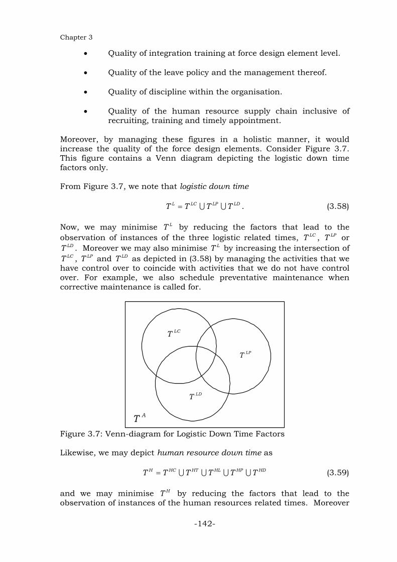
Moreover, by managing these figures in a holistic manner, it would increase the quality of the force design elements. Consider Figure 3.7. This figure contains a Venn diagram depicting the logistic down time factors only. From Figure 3.7, we note that logistic down time L LC LP LDT T T T= ∪ ∪ . (3.58) Now, we may minimise LT by reducing the factors that lead to the observation of instances of the three logistic related times, LCT , LPT or

LDT . Moreover we may also minimise LT by increasing the intersection of LCT , LPT and LDT as depicted in (3.58) by managing the activities that we

have control over to coincide with activities that we do not have control over. For example, we also schedule preventative maintenance when corrective maintenance is called for.

AT

LDT

LPT

LCT

Figure 3.7: Venn-diagram for Logistic Down Time Factors Likewise, we may depict human resource down time as H HC HT HL HP HDT T T T T T= ∪ ∪ ∪ ∪ (3.59) and we may minimise HT by reducing the factors that lead to the observation of instances of the human resources related times. Moreover


-143-

as was the case with the logistic environment we may also minimise HT by increasing the intersection of HCT , HTT , HLT , HPT and HDT as depicted in (3.59) by managing the activities that we have control over to coincide with activities that we do not have control over. Furthermore, we may depict up time by means of a Venn diagram to be U A L HT T T T= − ∪ (3.60) and we may then maximise UT in a similar fashion to that we have described for minimising LT . 7. CONCLUSION In this chapter we have researched the question:

If the relationships between a military strategy, its ends, ways and means, are quantified, and if the effectiveness of the force design elements is known, how shall that enable the quantification of the state’s ability to execute its military strategy?

We have shown that if the extent to which the relationships between a military strategy, its ends, ways and means exist, is quantified, and if the effectiveness of the force design elements is known, then we may deliver the several information sets to the management information system to enable decision-making regarding the following:

• Criteria for deciding on Combat Readiness.

• Quantification of risk management factors.

• Managing for the quality of a wide variety of management and leadership aspects.

Chapter 3

-144-

Documents

Weapon System Effectiveness - Unisauir.unisa.ac.za/bitstream/handle/10500/1527/03Chapter3.pdfThe measuring of weapon system effectiveness by using the systems-space reduces to the