Embed Size (px)
Citation preview

Optimal trim control of a high-speed craft by trim tabs/interceptors
Part I: Pitch and surge coupled dynamic modelling using sea trial data
Melek Ertogana,b,*, Philip A. Wilsonb, Gokhan Tansel Tayyarc, Seniz Ertugruld
a Maritime Faculty-Marine Engineering, Istanbul Technical University, Turkey
b Faculty of Engineering and the Environment, University of Southampton, U.K.
c Naval Architecture and Marine Engineering, Istanbul Technical University, Turkey
d Mechanical Engineering, Istanbul Technical University, Turkey
ABSTRACT
A pitch and surge coupled dynamic model of a high-speed craft is not available for dynamic trim control
applications in the literature. The existing fluid-structure interaction models of a high-speed craft are not adequate
for simulations and control applications, since they require a great deal of computation time, for example more than
20-40 sec. depending on a vessel particulars. Hence, in this work, we aimed to obtain a dynamic model of a high-
speed craft for surge and pitch motions. Then the obtained model will be utilized to design an automatic controller
which adjust the command signal on a high-speed craft to increase fuel efficiency, safety and comfort of passengers
in a vessel. The coupled pitch and surge motion of a high-speed craft with trim tabs/interceptors was modelled by
using full scale sea trial data. The linear parametric modelling using System Identification (SI) Methods and
Artificial Neural Network (ANN) modelling were carried out and the comparisons of both the training and
validation results are given. High correlation coefficients and low average values of absolute errors in surge and
pitch dynamics were obtained by using ANN Method. The ANN model can be improved for further control designs
on a marine vessel’s operations.
Keywords: high speed craft dynamics, trim tabs/interceptors, linear/nonlinear modelling, full-scale experiments,
system identification (SI), artificial neural network (ANN).
* Corresponding author at: Marine Engineering Faculty, Istanbul Technical University, Tuzla, Istanbul, Turkey. Phone: +90-533-3408113, fax: 90-216-3954500.
E-mail addresses: ertogan@ itu.edu.tr , [email protected] (M. Ertogan),[email protected] (P.A. Wilson), [email protected] (G.T. Tayyar),[email protected] (S. Ertugrul)
1
2
3
4
5
6
7
8
9
10
11
12
13
14
15
16
17
18
19
20
21
22
23
24
123456

1. INTRODUCTION
Marine vessels’ motions are generally determined by experimental tests, and direct numerical solutions based on
Navier-Stokes Equations by Computational Fluid Dynamics (CFD) (ITTC, 2011). There are many publications in
the field of dynamic modelling for displacement type of a ship. The dynamics of a high-speed craft are different
from displacement ships. It has displacement, semi-displacement, and planing characteristics according to Froude
numbers (Faltinsen, 2005; Fossen, 2011). In this study, it is aimed to model surge and pitch motions of a high speed
craft to be able to design dynamic trim controller during planing or semi-planing hull motion using existing trim
tabs/interceptors which controlled manually.
Initial studies of a hydrodynamic model for prismatic form of a high speed craft was done with experimental tests
for smooth and rough sea conditions (Savitsky, 1964; Savitsky and Brown, 1976). The linearized and empirical
equations of a high-speed craft in wave conditions were presented in detail (Lewandowski, 2003; Faltinsen, 2005).
A numerical analysis on vertical dynamics of a planing craft in calm sea and in waves was studied (Blake, 2000;
Blake and Wilson, 2001). A numerical simulation algorithm based on the finite volume discretisation was presented
for analysing 3D nonlinear high-speed vessels motion, and the steady-state forward motion of it was investigated
(Panahi, et al., 2009). An interceptor’s effectiveness on the hydrodynamic performance for a high-speed craft was
investigated (Karimi et al., 2013). The other hydrodynamic designs of interceptor/trim tabs were studied (Tasi and
Hwang, 2004; Luca and Pensa, 2012; Mansoori and Fernandes, 2016). Furthermore, an autonomous planning
watercraft test bed was developed to improve the controller technologies for a planning craft (Woelfel, et al., 2004;
Blank and Bishop, 2008).
In this study, even it is possible to achieve a dynamic model via CFD analysis, generating a dynamic model from sea
trials is preferred since it is more suitable for real time controller design. Therefore, the dynamic model in the form
of linear and nonlinear identifications are obtained from full scale sea trials that represent nonlinear, coupled surge
and pitch motion depending on the engine speed, trim tab/interceptor position and heave acceleration.
25
26
27
28
29
30
31
32
33
34
35
36
37
38
39
40
41
42
43
44
45
46
47
48
49

Modelling studies by SI in multidisciplinary area have shown a good level of accuracy according to empirical and
theoretical methods (Ljung, 1999). The studies on modelling by (SI) methods of marine vessels for controller design
purposes are limited. Early studies on identification of a ship’s steering dynamics were presented in detail (Aström
and Kallström, 1976). Manoeuvring motions of container ships were determined by SI methods afterward. Grey-
box modelling (Blanke and Knudsen, 2006), genetic algorithm (Sutulo and Soares, 2014), support vector regression
(Wang et al., 2015) and ANN (Simsir and Ertugrul, 2009) methods were used for identification of manoeuvring
motions. Identification for a heading autopilot of an autonomous in-scale fast ferry was studied (Velasco, et al.,
2013). An adaptive autopilot was designed to govern steering of a high speed unmanned personal watercraft by
using a grey-box identification model (Svendsen et al., 2012).
The parametric modelling of heave and pitch motions of fast ferries in the frequency domain was done by using a
simulator (Pintelon and Schoukens, 2004). The partial differential equation’s parameters of the coupled heave-pitch
motion of an icebreaker ship were identified by ANN (Haddara and Xu, 1999). Heave and pitch motions of a
planing craft with a transom flap in calm sea was modelled as steady-state method by using experimental data and
Savitsky’s method, and a controller was designed for reduction of porpoising instability in simulation studies
(Handa and Jing, 2006). A parametric model of heave, pitch and roll dynamics of a high-speed craft were defined in
the frequency domain according to wave excitations with different incidence angles between 90° and 180° by
using a simulator (Munoz-Mansilla et al., 2009). Then, the parametric model was utilized for stabilization control to
reduce motion sickness associated with heave, pitch and roll accelerations (Munoz-Mansilla et al., 2010).
The purpose of controller design may be to convert a manual trim system to an automatic controller, or to improve
an existing controller. The model should represent the dynamic behaviour of a high speed craft and be useful for
these control applications. This paper focuses on dynamic modelling of pitch and surge motion of a high-speed craft
so that an optimal trim controller could be designed based on the obtained model. The purposes of dynamic trim
control are fuel efficiency, safety, comfort of passenger in a vessel. Dynamic modelling of a high speed craft was
studied by SI, and ANN methods with sea trial data of Volcano71, in length 10.86m. The particulars of Volcano71
and experimental system setup are presented in Appendix A.
2. MOTIVATION
50
51
52
53
54
55
56
57
58
59
60
61
62
63
64
65
66
67
68
69
70
71
72
73
74
75

In a previous project, an advanced controller design of active fins for ship roll motion reduction was studied. Sea
trials in the coastal sea in Tuzla-Istanbul were done to collect data for experimental parameter identification to
establish a realistic roll motion equation for Marti, 16.5m in length. The advanced controller design was tested on
the Marti, as a full-scale application, after the real-time computer control was carried out for position control of the
hydraulic system. High performances were obtained from the real time tests. Considerable amount of experience
has been gained during these projects regarding data acquisition, signal processing, instrumentation, modelling and
real time control (Ertogan et al., 2015, 2016; Zihnioglu et al., 2015).
The optimal trim control of a high speed craft in nearly calm water is being studied in the current project. The
purpose of the automatic trim control is to improve fuel efficiency, safety and comfort of passengers in a marine
vessel. Devices such as trim tabs, interceptors, and sterndrive engines can be used to control the trim of a high speed
craft. These devices may be fixed or the system may be manually controlled and position of trim tabs/interceptor can
be changed by the captain based on experience. But it is difficult to control both longitudinal and lateral motions of
the high speed craft and manipulate the position of trim tabs/interceptors at the same time manually. Therefore, an
advanced algorithm is needed to automatically adjust the position of trim tabs/interceptor to maximize the speed for
a given throttle position. To be able to develop such advanced, reliable control algorithm, a model representing
coupled surge and pitch motions of the craft is required for simulation purposes. The aim of this study is to
investigate linear and nonlinear modelling techniques to find an adequate model to study the optimal trim controller
design which will increase the fuel efficiency.
Modelling methods are defined as three types; white-box modelling, grey-box modelling, and black-box modelling.
White-box modelling solves a series of combined differential equations. Grey-box modelling represents a known
plant system, but with limits to the possible excitation. Different parameterizations give significantly different model
quality for grey-box modelling, because some parameters may not be identifiable. Black-box modelling estimates
required variables based on the collected input-output data (Blanke and Knudsen, 2006; Wang et al., 2015).
In the literature, an article directly subjected on optimal trim control of a high speed craft could not be found. As
nearly related to our project topic, there are few articles which are generally about simulation studies on heave
motions’ reduction control, and manoeuvring control of a planing craft (Velasco et al., 2003; Handa and Jing, 2006;
76
77
78
79
80
81
82
83
84
85
86
87
88
89
90
91
92
93
94
95
96
97
98
99
100
101

Svendsen et al., 2012). Generally, a high speed craft was modelled as parametric identification from collecting
scaled-model test data for control purposes (Munoz-Mansilla et al., 2010).
In this project, the full-scale studies were preferred, because model test results suffer from scale effects (Woelfel et
al., 2004; Blanke and Knudsen, 2006). Intelligent, nonlinear methods for modelling were investigated for simulation
purposes, since designing and tuning of a controller algorithm via simulations requires less time, cost and effort
compared to real time sea trials.
3. EXPERIMENTAL MODELLING
The discrete-time non-linear model from sea trial data was desired. The Multi-Input-Multi-Output (MIMO) model
includes the three input signals as engine speed, interceptors/trim tabs’ position, and heave acceleration for each sea-
state condition, and the output signals as ship speed, and pitch motions, shown in Fig. 1.
Fig. 1. The input and output signals for a dynamic model of surge and pitch motions of a high-speed craft.
If an acceptable linear model could be obtained for the ship’s speed ranges standing for a high-speed craft, it would
be very useful for simulation purposes in controller design. Therefore, an attempt has been made to obtain linear
parametric models such as State-Space (SS) and ARX using well-established SI theory. However, it is known that
ship dynamics involve nonlinearities. Therefore, a non-linear modelling technic such as Neural Network needs to be
utilized. A decision should be made about the type of model depending on the results of both linear and non-linear
models.
In this paper, the full scale modelling of surge and pitch motions were studied by using the linear parametric models
of State-Space and ARX. In order to model the surge and pitch motions of a high-speed craft with the
interceptors/trim tabs by these methods, input signals should be persistently exciting. Collecting the sea trial data,
the linear parametric modelling and the nonlinear modelling methods are described in the following subtitles.
102
103
104
105
106
107
108
109
110
111
112
113
114
115
116
117
118
119
120
121
122
123

3.1 PERSISTENTLY EXCITING INPUT SIGNAL, AND SEA TRIAL DATA
Determining of proper input/ output signals for a physical system is significant, in order to use SI methods. The
input signals must be persistently exciting, so as to collect data that are sufficiently informative (Ljung, 1999).
One of the input signals for the dynamic model is a driver’s signal of a trim adjustment actuator. The interceptor and
the trim tab systems are operated with the PWM drivers. The PWM drivers were excited within the range of 10%-
100% duty cycle for the identification of the dynamic model. The trim adjustment actuators should be driven
periodically at approximately mid-PWM speeds for the identification, according to the experiences on the full-scale
experiments.
Other input signal for the experiments is the engine speed of the craft. The sea trials were done in increasing and
decreasing engine speeds at approximately in the range of 800-4000 rpm, according to setting the engine drivers’
commands, on condition that Volcano71 was on a straight course.
One of the trim adjustment actuators, the interceptors or the trim tabs, were operated periodically as mentioned
above in the sea trials. The sea states were recorded from the local meteorology. The sea states are determined
according to the World Meteorological Organisation (WMO) sea state code.
The order of excitation given with covariance matrix was calculated and it was verified that input signals were
persistently exciting to find models up to 50th order. The output signals are the ship’s speed, and the surge and pitch
motions, measured by the GPS and the IMU. In addition to the engine speed and the interceptors/trim tabs’ position
were chosen as inputs, the heave acceleration had to be added as the input signal to achieve a more reliable model.
The ship speed, pitch motion, acceleration of heave motion, manual command signal of the interceptors and the
engine speed, in sea state 1, 0 to 0.1m wave height, wave characteristics as ripples, are shown in Fig. 2. It can be
observed that the ship’s speed increases because of the interceptors in these conditions at the constant throttle
condition, engine speed at approx. 2600 rpm as shown in Fig. 3. It should be noted that variables are scaled to be
shown on the same figure.
124
125
126
127
128
129
130
131
132
133
134
135
136
137
138
139
140
141
142
143
144
145
146
Fig. 2. The ship speed, pitch angle, acceleration of heave motion, the interceptors’ position, the engine speed, in sea
state 1.
Fig. 3. The ship speed, pitch angle, heave acceleration, the interceptors’ position, in sea state 1, at the engine speed
approx. 2600 rpm.
The input and output signals from another sea trial, in sea state 2, 0.1 to 0.5m wave height, wave characteristics as
wavelets, and character of the sea swell as short, are illustrated in Fig. 4.
147
148
149
150
151
152
153
154

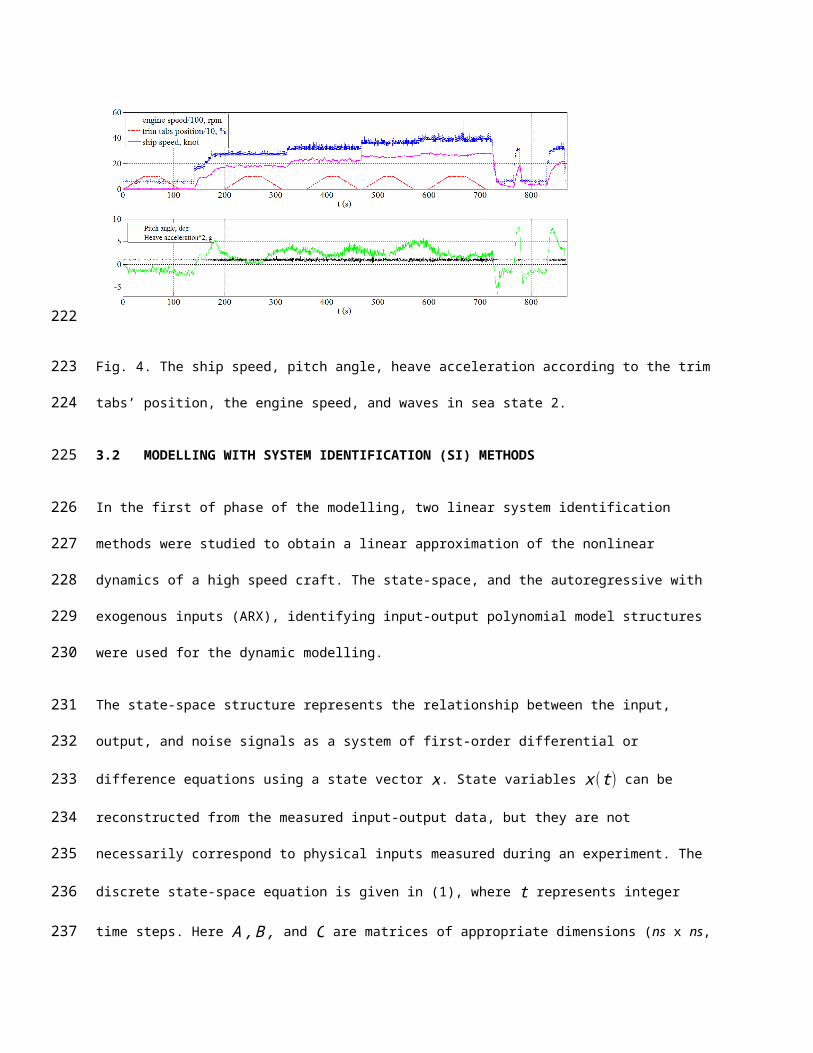
Fig. 4. The ship speed, pitch angle, heave acceleration according to the trim tabs’ position, the engine speed, and
waves in sea state 2.
3.2 MODELLING WITH SYSTEM IDENTIFICATION (SI) METHODS
In the first of phase of the modelling, two linear system identification methods were studied to obtain a linear
approximation of the nonlinear dynamics of a high speed craft. The state-space, and the autoregressive with
exogenous inputs (ARX), identifying input-output polynomial model structures were used for the dynamic
modelling.
The state-space structure represents the relationship between the input, output, and noise signals as a system of first-
order differential or difference equations using a state vector x. State variables x (t) can be reconstructed from the
measured input-output data, but they are not necessarily correspond to physical inputs measured during an
experiment. The discrete state-space equation is given in (1), where t represents integer time steps. Here A , B , and
C are matrices of appropriate dimensions (ns x ns, ns x mu, and my x ns, respectively, for an ns-dimensional state,
an mu-dimensional input, and an my-dimensional output). Θ is a vector of parameters that typically correspond to
unknown values of physical coefficients, and the like. The modelling is usually carried out in terms of state variables
x (t) that have physical significance, and then the measured outputs, y (t ) will be known combinations of the
states. Moreover, u(t ), we (t), and ve(t ) are the measured input data, the measurement noise, and the process
noise respectively. x0 represents the initial conditions (Ljung, 1999).
155
156
157
158
159
160
161
162
163
164
165
166
167
168
169
170
171
172

x (t +1 )=A (Θ ) x ( t )+B (Θ ) u ( t )+we (t )
y (k )=C (Θ ) x (k )+ve(k )
x (0 )=x0 (1)
The state-space model structure requires to be specified the model order, ns, the model structure configuration, and
the estimation options (Ljung, 2013). Some types of the model structure configuration are free parameterization, and
canonical parameterization. The free parameterization method estimates all constants of the system matrices. The
canonical parameterization method constructs a state-space system in a reduced parameter form where many entries
of the system matrices are fixed to zeros and ones. The free parameters are located in only a few the rows and
columns in the system matrices for the canonical parameterization method. The free parameters can be identified by
the companion form, the modal decomposition form, and the observability canonical form. The characteristic of
polynomial structure represents in the rightmost column of the A matrix for the companion form. The modal form
has a symmetry in the block diagonal elements of the state matrix A. The free parameters are located in the selected
rows of the system matrices for the observability canonical form.
The other types of the model structure configuration are structured parameterization, and completely arbitrary
mapping methods. Which entries of the system matrices to be estimated and which entries to be specified as fixed
can be chosen in the structured parameterization method. The structured estimation method is also referred to as
grey-box modelling. However, the relationships among state-space coefficients cannot be indicated for the
structured estimation approach. The grey-box modelling method permits to calculate dependencies among the
parameters of the system matrices.
In this study, the free parameterization, and the canonical parametrization methods were simulated as the modal
structures. In addition to these, the non-iterative, subspace method (Van Overschee and De Moor, 1996), and the
iterative, prediction error minimization estimation (Ljung, 1999) methods were chosen for the black-box modelling.
In addition to this, the polynomial ARX model was studied as another linear system identification method. The
discrete-time designation of the ARX model given in (2) is composed of a linear differential equation and error term.
In addition to these, it has model parameters to be determined. ARX model parameters were estimated from the
173
174
175
176
177
178
179
180
181
182
183
184
185
186
187
188
189
190
191
192
193
194
195
196
197

experimental data using the Least Squares Estimation (LSE) (Soderstrom and Stoica, 1989). In the ARX model, the
output of the system at a specific time is assumed to be linear combinations of the previous outputs and inputs, and
the current input. The multivariable ARX model with mu inputs and my outputs is given in (2) (Ljung, 1999, 2013).
Q ( z−1 ) y (t )=R ( z−1 ) u (t )+e(t ) (2)
where y is the output, u is the input, e (t) is the modelling error, t represents integer time steps, Q(z−1) and
R(z−1) are model parameters to be estimated using the experimental data. Q(z−1) is an my x my matrix whose
entries are polynomials in the delay operator z−1. It can be represented as given in (3). The matrix form of Q(z−1)
is given in (4).
Q ( z−1 )=I my+Q1 ( z−1 )+…+Qna(z−na) (3)
Q ( z−1 )=[ q11 (z−1) ⋯ q1 my (z−1)⋮ ⋱ ⋮
qmy 1(z−1) ⋯ qmymy (z−1)] (4)
The entries qkj are polynomials in the delay operator z−1 represented as
qkj ( z−1 )=δkj+qkj1 ( z−1 )+…+qkj
nakj (z−nakj) (5)
The polynomial given in (5) describes how old values of output number j affect output number k. Where δ kj is the
kronecker-delta which equals 1 when k=j, otherwise, it is 0. Similarly, R(z−1) is an my x mu matrix given in (6), or
(7) with (8).
R ( z−1 )=R0+R1 ( z−1 )+…+Rnb(z−nb) (6)
R ( z−1 )=[ r11(z−1) ⋯ r1 mu( z−1)⋮ ⋱ ⋮
qmy 1(z−1) ⋯ qmymu(z−1)] (7)
198
199
200
201
202
203
204
205
206
207
208
209
210
211
212
213
214

rki ( z−1 )=rki1 ( z−nk ki)+…+rki
nbki( z−nk ki−nbki+1) (8)
The delay from input number i to output number k is nk ki. na , nb∧nk are the orders of the output, input and input-
output delay, respectively. na is a matrix whose kj-element nakj, while the ki-elements of nb an nk are nbki and
nk ki, respectively.
The results of the state-space, and the ARX models’ simulations are described in detail in Section 5.
3.3 NEURAL NETWORK MODELLING
Artificial Neural Networks (ANN), with ability to learn complicated relations from Multi-Input and Multi-Output
(MIMO) imprecise data, can be used to model non-linear system dynamics. ANN can be preferred to apply because
of its advantages: to learn, and generalize from training data then, it estimates from the given data, and makes
associations between the validation data and the training data (Hagan et al., 2014; Demuth et al., 2013).
ANN consists of simple processors called neurons. A simple neuron has three sections; synapses, collector, and
activation functions. It receives its input signal through other neurons. Each input signal, ‘x’ is weighted by a weight
‘w’, and the weight is updated with synaptic learning. The weighted total is calculated by using the weights, and the
input signals, given in (9), where, x is input signal, w is weight, θ=x0w0 is bias value, and net is weighted sum.
net=∑ x i wi=¿θ+x1w1+…+xm wm ¿ (9)
The two most used activation functions are logistic function, and hyperbolic tangent function, and both are
sigmoidal functions. The sigmoidal function limits the domain of output to (-1, 1) or (0, 1). The output of the
activation function is given (10), where f ( . ) is the activation function, y is the output signal (Du and Swamy,
2006).
y=f (net) (10)
A multi-layer feed-forward ANN structure is illustrated in Fig. 5. The layers are placed as an input layer, hidden
layers, an output layer. The hidden layers represent the non-linear structure of the ANN. In each layer, there may be
215
216
217
218
219
220
221
222
223
224
225
226
227
228
229
230
231
232
233
234
235
236
237
more than one neuron. The neurons pass the inputs of the neurons from each previous layer, but they do not have
connections within the neurons in the same layer. Assume that there are M layers, each layer having
Lm ,m=1,2 ,…, M , neurons. The weights from the (m-1)th layer to mth layer are defined by Wm-1. In addition to
these, the bias, output, and activation function of the ith neuron in the mth layer are denoted θim , o i
m, and f im(.)
respectively. The relations from Fig. 5 are given (11), and (12) (Du and Swamy, 2006).
net dm=[W m−1 ]T od
m−1+θm (11)
odm=f m (net d
m) (12)
for m=2,3 ,…, M , where the subscript d corresponds to the dth example, net dm=(net d , 1
m ,…,net d , Lm
m )T , Wm-1 is a
Lm−1−by−Lm matrix, odm−1=(od ,1
m−1 , …, od ,Lm−1
m−1 )T , θm=(θ1m ,…,θLm
m )T is the bias vector. f m(.) applies f im(.)
to the ith component of the vector.
Fig. 5. Multilayer ANN structure
The Backpropagation (BP) algorithm is a learning method, known as the Least Mean Square (LMS) algorithm,
which needs both the inputs and the targets to compute optimum weights and biases. An error is calculated by the
comparisons between the outputs and the targets in the training process. This error signal is propagated backward
the network while the BP algorithm utilizes a gradient descent technique to minimize an objective function. The
objective function is the Mean Square Error (MSE) between the network outputs, yd and the targets, yd for all the
training data pairs( xd , yd )∈S, given in (13) where N is the size of the sample data.
238
239
240
241
242
243
244
245
246
247
248
249
250
251
252
253
254
255
256
257

E= 12 N ∑
d ∈S‖ yd− yd‖
2=¿ 12 N ∑
d ∈Sε2¿ (13)
The error function E is minimized by the gradient descent method, given in (14). Hence, the weights, and the biases
can be updated.
∆ W =−ζ ∂ E∂ W (14)
Where the matrix W includes all the weights, W m−1 and the biases, θm. The degree of influence of the gradient on
the weights and biases at each iteration is determined by learning rate, ζ . In practice, ζ is usually chosen to be
0<ζ <1, so the weight updates do not overshoot the minimum of the error surface.
There are generally two training styles for the ANN structure as the incremental (online), and the batch (offline)
methods. The network weights and biases are updated after each presented sample data, in the incremental training.
However, the weights and biases are updated after all the training data is presented for the batch training. In this
study, the batch training method was preferred to model the couple of surge and pitch dynamics of a high speed
craft, so a comprehensive model could be obtained by taking into consideration all the training data for each sea
state.
The BP can be performed using different types of optimization techniques. In this paper, the gradient descent with
momentum and adaptive learning rate backpropagation, and Levenberg-Marquardt, which is proposed to solve non-
linear least-square problem, methods were applied to model a nonlinear dynamics of a high speed craft.
The standard steepest descent algorithm is the simplest but the slowest in convergence to train the ANN model, so
two modifications called adaptive learning rate and momentum are also applied to improve the performance of
steepest descent method. If the learning rate, ζ is too small, the algorithm takes a long time to converge, while a too
large learning rate makes the algorithm unstable. An adaptive learning rate is used for a solution to this problem. In
the adaptive learning method, the learning rate is not a constant, it updates according to a new error in each iteration.
In addition to this, a momentum term is added to improve the BP algorithm, given in (15).
258
259
260
261
262
263
264
265
266
267
268
269
270
271
272
273
274
275
276
277
278
279
280
281
282
ΔW (t )=−ζ ∂ E∂ W
+ϱ ∆ W (t−1) (15)
where ϱ is the momentum factor, is usually 0<ϱ≤ 1. The momentum term provides to reduce the sensitivity of the
network to fast changes of the error surface. It effectively smoothes oscillations and accelerates convergence.
The BP algorithm is slow to converge when the error surface is flat along a weight dimension. Second-order
optimization techniques have a strong theoretical basis and provide faster convergence. Second-order methods make
use of the Hessian matrix H, given in (16).
H ( t )=∂2 E∂ w2 ¿t (16)
Where H is the second-order derivative of the error E with respect to the Dw – dimensional weight vector w . The
weight vector is obtained by concatenating all the weights and biases of a network. The Hessian matrix, Dw x Dw
contains information as to how the gradient changes in different directions of the weight space. It can be applied to
the BP algorithm.
The Levenberg-Marquardt (LM) method provides to eliminate the possible singularity of H by adding a small
identity matrix to it. The method is derived by minimizing the quadratic approximation to E (w ) subject to the
constraint that the search step length ‖d( t )‖ is within a trust region at step t. The second-order Taylor
approximation of E (w ) is given in (17). The gradient vector is given by g (t )=∇E (w (t )) (Du and Swamy, 2006).
E (w (t )+d ( t ) )=E (w (t ) )+g (t )T d (t )+12
dT (t ) H (t )d (t ) (17)
Therefore, the LM method is represented by (18).
∆ w(t)=−( H (t )+ξ (t ) I )−1 J T ( t ) ε (t) (18)
where ξ (t) is a small positive value. It controls the size of the trust region. The Jacobian matrix is defined as
J (w )=∂ ε ¿¿.
283
284
285
286
287
288
289
290
291
292
293
294
295
296
297
298
299
300
301
302
303
304

The implementations of the linear system identification methods as the State-Space (SS) and ARX, and Neural
Network modelling are described in detail, and the results of the modelling process are given in Section 4.
4. PERFORMANCE EVALUATION OF MODELS
The sea trial data collected with 0.1 s sampling period in calm sea condition as sea state 1, and in small irregular
wave sea condition as sea state 2 were used for the modelling studies. The input variables; the trim tabs/interceptor
position, the engine speed and heave motion acceleration, the output variables; ship speed and surge motion were
recorded during the sea trials with Volcano71. The heave motion acceleration as an input signal was added to
increase the pitch motion prediction performance after initial attempts. The experimental data was revised taking
into account the delay time of the GPS receiver. The delay time of the GPS was determined as 2 s empirically. The
dynamic models of a high speed craft were obtained by using the SS and ARX as linear parametric models, and
ANN nonlinear model. After the models had been identified by the training data sets, these models were validated
using another set of data. There are total of 3150 samples of data collected during the same sea trail for the sea state
1. Then 2050 data were used for training and 1100 were used for validation. Also, there are total of 13580 samples
of data collected during the same sea trail for the sea state 2. Then 8600 data were used for training and 4980 were
used for validation.
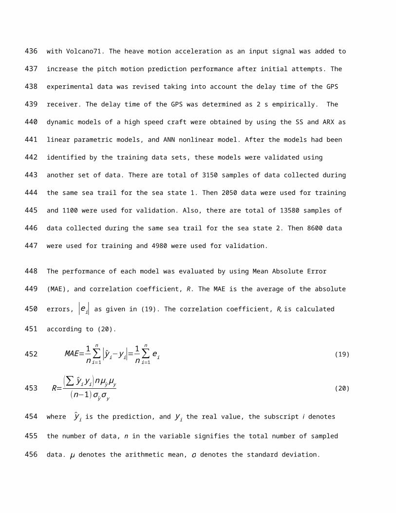
The performance of each model was evaluated by using Mean Absolute Error (MAE), and correlation coefficient, R.
The MAE is the average of the absolute errors, |e i| as given in (19). The correlation coefficient, R, is calculated
according to (20).
MAE=1n∑i=1
n
|y i− y i|=1n∑i=1
n
ei (19)
R=(∑ y i y i )n μ y μy
(n−1)σ y σ y
(20)
where y i is the prediction, and y i the real value, the subscript i denotes the number of data, n in the variable
signifies the total number of sampled data. μ denotes the arithmetic mean, σ denotes the standard deviation.
305
306
307
308
309
310
311
312
313
314
315
316
317
318
319
320
321
322
323
324
325
326
327

In the SS modelling study, the free parameterization, and the canonical parametrization methods were simulated as
the model structures. In addition to these, the non-iterative, subspace method, and the iterative, prediction error
minimization estimation methods were practised for the linear parametric modelling. Moderately good results from
the SS model was obtained by using the free parametrization model structure, and the subspace method for the both
of the sea conditions, but the ns orders of the SS models for the sea state 1, and the sea state 2 were determined as 4
and 5, respectively.
Different model orders were tried for the sea state 1 and 2 conditions in the ARX modelling studies. The model for
the sea state 1 condition with orders nakj=3 for all the outputs, and nbki=2 for all the inputs was obtained, and it
reasonably well fitted to the real data. Another model for the sea state 2 condition with order nakj=5 for all the
outputs, and nbki=3 for all the inputs produced successful results in predicting the dynamics of the high speed
craft. The delay time nk ki=1 for both of the sea conditions was determined, because the experimental data was
revised taking into account the delay time of the GPS receiver. The structures of the dynamic models will be called
ARX321 for the sea state 1, and ARX531 for the sea state 2 conditions.
However, the best performances were attained by ANN models. The accuracy of the prospective model is essential,
because small trim angles of high speed craft will be important for the implementations of optimal trim control
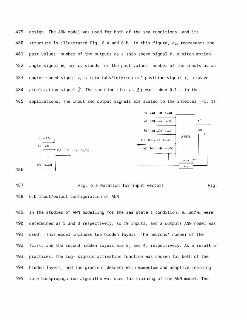
design. The ANN model was used for both of the sea conditions, and its structure is illustrated Fig. 6.a and 6.b. In
this figure, nout represents the past values’ number of the outputs as a ship speed signal V, a pitch motion angle signal
φ, and nin stands for the past values’ number of the inputs as an engine speed signal v, a trim tabs/interceptor’
position signal τ , a heave acceleration signal Z. The sampling time as ∆ t was taken 0.1 s in the applications. The
input and output signals are scaled to the interval [-1, 1].
328
329
330
331
332
333
334
335
336
337
338
339
340
341
342
343
344
345
346
347

Fig. 6.a Notation for input vectors Fig. 6.b Input/output configuration of ANN
In the studies of ANN modelling for the sea state 1 condition, nout and nin were determined as 5 and 3 respectively, so
19 inputs, and 2 outputs ANN model was used. This model includes two hidden layers. The neurons’ number of the
first, and the second hidden layers are 5, and 4, respectively. As a result of practices, the log- sigmoid activation
function was chosen for both of the hidden layers, and the gradient descent with momentum and adaptive learning
rate backpropagation algorithm was used for training of the ANN model. The ship’s speed, and the pitch motion
angle comparisons of the linear parametric models as the SS and the ARX, and the ANN as non-linear model are
illustrated for both of the training and the validation data sets in Fig. 7, and 8, respectively. In addition to this, the
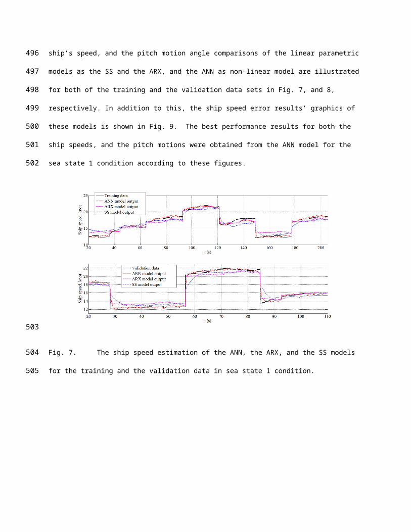
ship speed error results’ graphics of these models is shown in Fig. 9. The best performance results for both the ship
speeds, and the pitch motions were obtained from the ANN model for the sea state 1 condition according to these
figures.
348
349
350
351
352
353
354
355
356
357
358
359
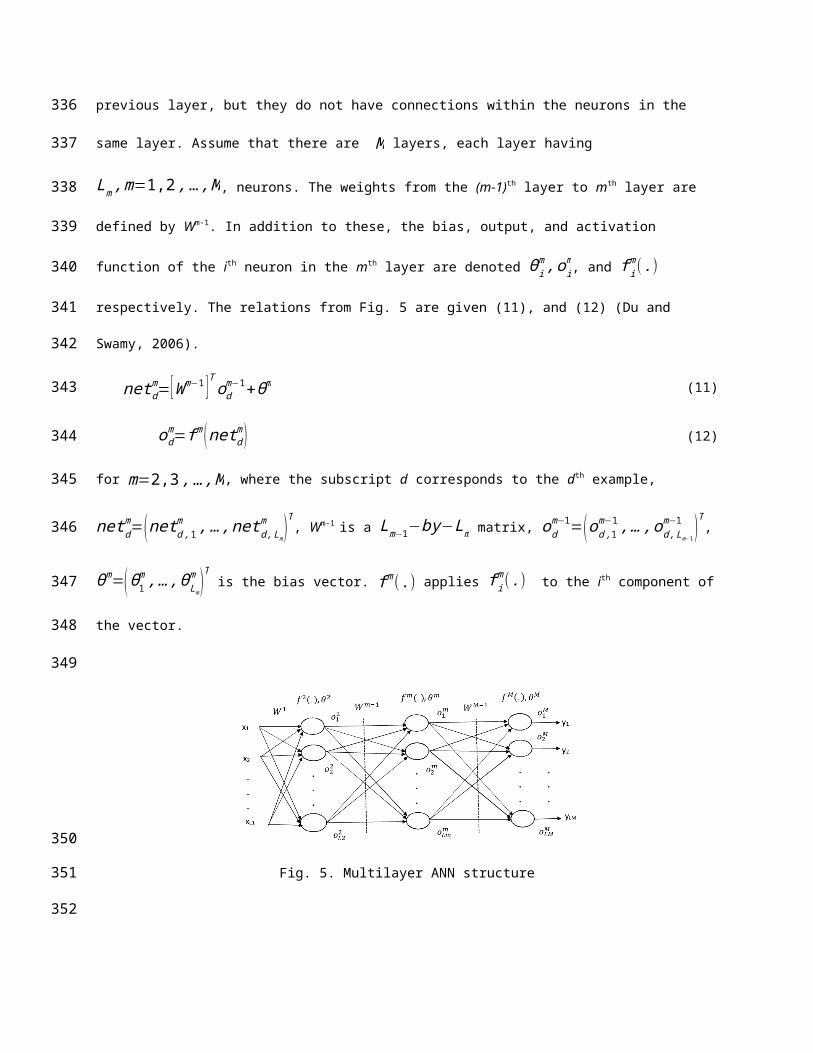
Fig. 7. The ship speed estimation of the ANN, the ARX, and the SS models for the training and the validation data
in sea state 1 condition.
Fig. 8. The pitch angle estimation of the ANN, the ARX, and the SS models for the training and the validation data
in sea state 1 condition.
360
361
362
363
364
365

Fig. 9. The ship speed estimation error of the ANN, the ARX, and the SS models for the training in sea state 1
condition.
In the ANN modelling applications for the sea state 2 condition, the same as the sea state 1 condition, the ANN
model consists of two hidden layers. The neurons’ number of the first, and the second hidden layers are 5, and 4,
respectively. This ANN model was trained by the Levenberg-Marquardt algorithm. nout =7, nin =5 were selected, so
29 inputs, and 2 outputs ANN model was used. The log- sigmoid activation function was used for both of the hidden
layers. The ship’s speed, and the pitch motion angle results of the linear parametric models as the SS and the ARX,
and the ANN non-linear model are shown for both of the training and the validation data sets in Fig. 10, and 11,
respectively for the sea state condition 2. The outputs as the ship speed, and the pitch motion angle from the ARX
model resulted with better fitting values than the SS model. The best performance results for both the ship speeds,
and the pitch motions were obtained from the ANN model according to these figures.
366
367
368
369
370
371
372
373
374
375
376
377
Fig. 10. The ship speed estimation of the ANN, the ARX, and the SS models for the training and the validation data
in sea state 2 condition.
Fig. 11. The pitch motion angle estimation of the ANN, the ARX, and the SS models for the training and the
validation data in sea state 2 condition.
The performance values for both of the sea state conditions were also analysed by the correlation coefficient R, and
the average absolute value MAE, these values are given in Table 1 and 2, respectively. In the ANN model studies,
378
379
380
381
382
383
384
385

the average values of absolute errors MAE for the ship speed were calculated approximately 0.3 knot for both of the
testing and validation data in the calm sea condition as sea state 1. In the irregular sea condition as the sea state 2,
the MAE values of the ship speed outputs of the ANN model were obtained as approximately 0.5 knot. In addition
these, the MAE values of the pitch motion outputs of the ANN model in the both of the sea conditions are
approximately0.50. These MAE values, and the correlation coefficients R of the ANN model are acceptable to
develop an optimal trim controller via simulations.
Table 1: The correlation coefficients (R) of the ship speed and pitch motion angle for the SS, the ARX, and the
ANN models in sea state 1 and sea state 2 conditions.
Sea state 1 Sea state 2
Ship speed, knot Pitch Angle, deg. Ship speed, knot Pitch angle, deg.
Training data
Validation data
Training data
Validation data
Training data
Validation data
Training data
Validation data
SS 0.93 0.94 0.68 0.57 0.89 0.85 0.73 0.48
ARX 0.95 0.97 0.75 0.68 0.92 0.93 0.88 0.66
ANN 0.99 0.99 0.83 0.80 0.99 0.96 0.96 0.87
Table 2: The average of absolute errors (MAE) of the ship speed and pitch motion angle outputs of the SS, the ARX,
and the ANN models in sea state 1 and sea state 2 conditions.
Sea state 1 Sea state 2Ship speed, knot Pitch angle, deg. Ship speed, knot Pitch angle, deg.
Training data
Validation data
Training data
Validation data
Training data
Validation data
Training data
Validation data
SS 0.94 0.70 0.88 0.78 1.4 1.1 1.2 0.85ARX 0.85 0.51 0.75 0.67 0.96 0.88 0.83 0.66ANN
0.30 0.32 0.58 0.56 0.52 0.56 0.47 0.45
5. CONCLUSIONS AND FUTURE STUDIES
386
387
388
389
390
391
392
393
394
395
396
397
398

In this research, three different dynamic models were obtained representing surge and pitch motions of a high-speed
craft for simulation and control design purposes. Experimental data were collected from an instrumented high speed
craft. Inputs and outputs of the model were carefully selected, orders and delays were determined to obtain a reliable
model using the System Identification Theory. The trim tap/interceptor position and ship speed have been manually
changed so that the system dynamics were excited. By utilizing experimental data ARX and SS models were
identified and compared with ANN models. When figures are examined closely, all models well represent the
system’s dynamic behaviour. As can be seen from the Figures and Tables, ANN achieved smaller errors than ARX
and SS in all cases. Therefore, the ANN model can be used for the simulation and the controller design purposes
such as optimal trim control which will the next step and explained in a follow up paper, as Part II.
These modelling approach can be extended to include other motions such as manoeuvring or heave motion reduction
control purposes.
ACKNOWLADGEMENTS
Authors would like to thank I.T.U. Scientific Research Funds for partial support (project number: 37491) and The
Republic of Turkey Ministry of Industry and Trade, 1507 - SME RDI (Research, Development & Innovation) Grant
Programme for the support provided for the project numbered 7141282.
The author is also grateful to the University of Southampton for facilitating the research.
7. REFERENCES
Aström, K.J., Kallström, C.G., 1976. Identification of ship steering dynamics. Automatica, Vol. 12, pp. 9-22.
Blake, J.I.R., 2000. Investigation into the vertical motions of high speed planing craft in calm water and in waves.
PhD thesis, Faculty of Applied Science and Engineering School of Engineering Sciences, University of
Southampton.
Blake, J.I.R., Wilson, P.A., 2001. An analysis of planning craft vertical dynamics in calm water and waves. Royal
Institution of Naval Architects, UK, Vol. 1, pp. 77-90.
399
400
401
402
403
404
405
406
407
408
409
410
411
412
413
414
415416
417
418
419
420
421
422
Blank, J., Bishop, B.E., 2008. In-Situ modeling of a high-speed autonomous surface vessel. 40th Southeastern
Symposium on System Theory, 2008.
Blanke, M., Knudsen, M., 2006. Efficient parameterization for grey-box model identification of complex physical
systems. 14th IFAC Symposium on Identification and System Parameter Estimation, Newcastle, Australia,
Vol. 39, pp. 338-343.
Demuth, H.B., Beale, M.H., Hagan, M.T., 2013. Neural Network ToolboxTM, Version 8.0.1, The MathWorks, Inc.
Du, K.-L., Swamy, 2006. Neural networks in a softcomputing framework, Springer-Verlag London Ltd.
Ertogan, M., Tayyar, G.T., Karakas, S., Ertugrul, S., 2015. Review of measurement and real-time control systems
for marine applications. The 4th International Conference on Advanced Model Measurement Technologies for
the Maritime Industry, Istanbul, Turkey, pp. 72-p.1-p.20.
Ertogan, M., Ertugrul, S., Taylan, M., 2016. Application of particle swarm optimized PDD2 control for ship roll
motion with active fins. IEEE-ASME Transactions on Mechatronics, Vol. 21, pp. 1004-1014.
Faltinsen, O.M., 2005. Hydrodynamics of high-speed marine vehicles, Cambridge University Press, Cambridge,
UK.
Fossen, T.I., 2011. Handbook of marine craft hydrodynamics and motion control, First Edition. John Wiley & Sons
Ltd.
Haddara, M.R., Xu, J., 1999. On the identification of ship coupled heave-pitch motions using neural networks.
Ocean Engineering, Vol. 26, pp. 381-400.
Hagan, M.T., Demuth, H.B., Beale, M.H., De Jesus, O., 2014. Neural Network Design, Martin Hagan, 2nd edition,
ebook.
Handa X., Jing S., 2006. Feedback stabilization of high-speed planing vessels by a controllable transom flap. IEEE
Journal of Oceanic Engineering, Vol. 31, No:2, pp. 421-431.
International Towing Tank Conference (ITTC), 2011. The seakeeping committee on final report and
recommendations to the 26th ITTC. In: Proceedings of the 26th ITTC, vol. 1, pp. 183–245
423
424
425
426
427
428
429
430
431
432
433
434
435
436
437
438
439
440
441
442
443
444
445
446
International Towing Tank Conference (ITTC), 2011a. The specialist committee on computational fluid dynamics—
final report and recommendations to the 26th ITTC. In: Proceedings of the 26th ITTC, vol. 2, pp. 337–377.
Karimi, M.H., Seif, M.S., Abbaspoor, M., 2013. An experimental study of interceptor’s effectiveness on
hydrodynamic performance of high-speed planning craft. Polish Maritime Research, Vol. 20, pp. 21-29.
Lewandowski, E.M., 2003. The dynamics of marine craft: maneuvering and seakeeping, Advanced Series on Ocean
Engineering, Vol.22.
Ljung, L., 1999. System identification: theory for the user. Prentice Hall, Second Edition.
Ljung, L., 2013. System identifiction toolboxTM for use with MATLAB. User’s Guide Version 8.3, The MathWorks,
Inc.
Luca, D., and Pensa, F., 2012. Experimental Investigation on Conventional and Unconventional Interceptors. The
Transactions of the Royal Institution of Naval Architects. Part B, International Journal of Small Craft
Technology, Vol. 154, pp. 65-72.
Mansoori, M., and Fernandes, A. C., 2016. The Interceptor Hydrodynamic Analysis for Controlling the Porpoising
Instability in High Speed Crafts. Journal of Applied ocean research, Vol. 57:40-51.
Munoz-Mansilla, R., Aranda, J., Manuel Diaz, J., De La Cruz, J., 2009. Parametric model identification of high-
speed craft dynamics. Ocean Engineering, Vol. 36, pp. 1025-1038.
Munoz-Mansilla, R., Aranda, J., Diaz, D.C., 2010. Robust control for high-speed using QFT and eigenstructure
assignment. IET Control Theory & Applications, Vol. 4, pp. 1265-1276.
Panahi, R., Jahanbakhsh, E., Seif, M.S., 2009. Towards simulation of 3D nonlinear high-speed vessels motion.
Ocean Engineering, Vol. 36, pp. 256-265.
Pintelon, R., Schoukens, J., 2004. Discussion on: “identification of multivariable models of fast ferries”. European
Journal of Control, Vol. 10, pp. 199-202.
Savitsky, D., 1964. Hydrodynamic design of planing hulls. Marine Technology, Vol. 1, pp. 71-95.
Savitsky, D., Brown, P. W., 1976. Procedures for hydrodynamic evaluation of planning hulls in smooth and rough
Water. Marine Technology, Vol. 13, No.4, pp. 381-400.
447
448
449
450
451
452
453
454
455
456
457
458
459
460
461
462
463
464
465
466
467
468
469
470
471
Simsir, U., Ertugrul, S., 2009. Prediction of manually controlled vessels’ position and course navigating in narrow
waterways using artificial neural networks. Applied Soft Computing, Vol. 9, No. 1217-1224.
Soderstrom, T., Stoica, P., 1989. System identification. Prentice-Hall, Hertfordshire, UK.
Sutulo, S., Soares, C.G., 2014. An algorithm for offline identification of ship manoeuvring mathematical models
from free-running tests. Ocean Engineering, Vol. 79, pp. 10-25.
Svendsen, C.H., Holck, N.O., Galeazzi, R., Blanke, M., 2012. L1 adaptive manoeuvring control of unmanned high-
speed water craft. Proceedings of the 9th IFAC Conference on Manoeuvring and Control of Marine Crafts, pp.
144-151.
Tasi, F. J., and Hwang, J. L., 2004. Study on the Compound Effects of Interceptor with Stern Flap for Two Fast
Monohulls. IEEE Xplore Conference: Oceans '04. MTTS/IEEE Techno-Ocean '04, Taiwan, Vol. 2, pp. 1023 -
1028.
Van Overschee, P., B. De Moor, 1996. Subspace identification of linear systems: theory, implementation,
applications. Springer Publishing.
Velasco, F.J., Lopez, E., Rueda, T.M., Moyano, E., 2003. Classical controllers to reduce the vertical acceleration of
a high-speed craft. European Control Conference, Cambridge, UK, pp. 1923-1927.
Wang X., Zou Z., Hou X., Xu F., 2015. System identification modeling of ship manoeuvring motion based on –
support vector regression. Journal of Hydrodynamics, 27(4), 502-512.
Woelfel, G.A., Ehrhardt, B.J., Bishop, B.E., 2004. Development of an autonomous planning watercraft test bed.
Proceedings of the Thirty-Sixth Southeastern Sysmposium, pp. 285-289.
Zihnioglu, A., Ertogan, M., Tayyar, G.T., Karakas, C.S., Ertugrul, S., 2015. Modelling, simulation and controller
design for hydraulically actuated ship fin stabilizer system. The 3rd International Conference on Control,
Mechatronics and Automation, Bercelona, Spain, ICCMA, Vol. 42, pp. 01003-p.1-p.6.
APPENDIX A. EXPERIMENTAL SYSTEM SETUP
Volcano71 is a high speed craft with a deep V form. Its profile view is given in Fig. A.1. The interceptor, and the
trim tab systems were installed for the real-time applications, as shown in Fig. A.2. The trim of the sterndrive
472
473
474
475
476
477
478
479
480
481
482
483
484
485
486
487
488
489
490
491
492
493
494
495
496
systems of the gasoline engines can be manually controlled by a hydraulic assisted system. These manual systems
can be controlled by an algorithm when the trim system becomes automatic.
The other particulars of Volcano71 are as follows: length overall LOA=10.86m, length on the waterline LWL=9.4m,
beam B=3.3 m, depth D=1.15 m, deadrise angle β=16°. Hydrostatic characteristics of it are displacement ∆=5.35
tons, draft T=0.45 m, metacentric height GM=0.64 m, natural period w0=3 s. Volcano71 has a 2x385 BHP
sterndrive twin engine reaching a speed up to 40 knots with the installed propellers.
Fig. A.1. Profile view of Volcano71.
The blade size and stroke of the interceptor’s are 430mm, and 50mm, respectively. The size of the trim tab’s plate of
the each engine is 450mm x 250mm. The Pulse Width Modulation (PWM) drivers were provided for the interceptor,
trim tab systems, and sterndrive systems.
a) b)
Fig. A.2. a) The technical drawing of the interceptor, and the trim tab systems, b) they were mounted on Volcano71
having the sterndrive engines.
497
498
499
500
501
502
503
504
505
506
507
508
509
510

A computer having a quad-core, 3.2 GHz processor, and 8 GB RAM has been used for laboratory and sea trial
works. An industrial embedded microprocessor unit with I/O electronic cards has been used for measurement and
control. An inertial measurement unit (IMU), including triaxial accelerometer, gyroscope, magnetometer, was
chosen to measure the ship’s 3-axis rotational and linear motions. The measurement range of the IMU’s outputs are
±4 g with 12-bit reading per axis, and ± 250°/ s with 16-bit reading per axis. . Also, a GPS was used, and its data
output rate is 1 Hz to 10 Hz. The GPS and the IMU have been used for data acquisition for modelling, and designing
the controller.
The GPS was utilized and considered as sole sensor for final prototype. A pair of electronic sensors for measuring
fuel flow and, a flow meter were also installed on the ship during experimental stage. The communication interface
of these sensors is with NMEA 2000 protocol.
Volcano71 was launched, after the experimental equipment setup was completed. The data was collected from sea
trials in Tuzla-Istanbul in order to obtain a coupled pitch and surge dynamic model. The next subsection describes
the data acquisition stage.
511
512
513
514
515
516
517
518
519
520
521
522
523
524