Comparative Evaluation of Deferred and Forward Shading Techniques in Terms of

Real Time Applications in Computer Games

Mark James SimpsonBSc(Hons) Computer Games Technology

2006/2007

0305318

Table of Contents

TABLE OF CONTENTS I

ABSTRACT III

ACKNOWLEDGEMENTS IV

CHAPTER 1 : PREVIOUS WORK 1

1.1 FORWARD SHADING 11.2 DEFERRED SHADING 21.3 RESEARCH QUESTION 4

CHAPTER 2 : ORGANISATION 5

CHAPTER 3 : PREVIOUS WORK 1

3.1 DEFERRED SHADING 13.2 FORWARD SHADING 2

3.2.1 Single Pass, Multiple Light (SPML) 23.2.2 Multiple Pass, Multiple Light (SPML) 2

3.3 DEFERRED SHADING 43.4 CHOOSING A SHADING MODEL 5

CHAPTER 4 : METHODS 7

4.1 CHAPTER STRUCTURE 74.2 COMMON FUNCTIONALITY 8

4.2.1 Set Representation 84.2.2 View Frustum Culling & Intersection Tests 84.2.3 Primitive Sorting 84.2.4 Building Shadow Casting Sets 94.2.5 Shadow Map Generation 11

4.3 DEFERRED SHADING 114.3.1 G-Buffer Format 114.3.2 G-Buffer Pass 124.3.3 Tangent Space Normal Mapping 134.3.4 Accessing the G-Buffer 144.3.5 Ambient lighting & Emissive Term 154.3.6 Shadow mapping 154.3.7 Directional lights 164.3.8 Localised Lighting 174.3.9 Omni-directional Lights 224.3.10 Spotlights 224.3.11 Skybox 224.3.12 Post Processing & Effects (Extensibility) 23

4.4 FORWARD SHADING 244.4.1 Light and Illumination Sets 244.4.2 Depth, Ambient & Emissive 244.4.3 Further lighting 254.4.4 Shadow mapping 264.4.5 Directional Lights 264.4.6 Localised Lighting 264.4.7 Omni-directional Lights 274.4.8 Spotlights 274.4.9 Post Processing & Effects 27

4.5 MEASURING PERFORMANCE 274.6 SCENES 28

4.6.1 Exterior Scene 284.6.2 Interior Scene 29

Page I

CHAPTER 5 : RESULTS 30

5.1 PERFORMANCE 305.1.1 Exterior Scene 305.1.2 Interior Scene (Shadows Enabled) 315.1.3 Interior Scene (Shadows Disabled) 31

5.2 NUMBER OF LIGHTS & SCREEN COVERAGE 325.2.1 One spot light 325.2.2 Two spotlights, overlapping (camera pointing at overlap) 32

5.3 DEFERRED SHADING STENCIL LIGHTING OPTIMISATION: 325.4 FORWARD SHADING ILLUMINATION SETS: 335.5 IMAGE FIDELITY 34

CHAPTER 6 : ANALYSIS 35

6.1 BATCHING 356.2 RENDERING PERFORMANCE 36

6.2.1 Performance & Screen Space Coverage 376.2.2 Vertex Transformation Costs 376.2.3 Optimisations 38

6.3 IMAGE FIDELITY 386.4 EXTENSIBILITY 38

CHAPTER 7 : CONCLUSION 39

7.1 SUMMARY 397.2 CONCLUSIONS 397.3 RECOMMENDATIONS FOR FUTURE WORK 40

APPENDIX A : PROJECT PROPOSAL 42

APPENDIX B : SELECTING A G-BUFFER FORMAT 49

APPENDIX C : CREATING LIGHT VOLUMES 50

APPENDIX D : THE PHONG LIGHTING MODEL 53

APPENDIX E : NVIDIA NVPERFHUD 57

APPENDIX F : PC SPECIFICATION 57

APPENDIX G : THE SHADING DEMO 58

GLOSSARY 59

REFERENCES 61

Bibliography 64

Page II

Abstract

This project characterises the various strengths and weaknesses of the deferred and multi-pass forward shading rendering techniques. Deferred shading is a technique that allows lighting to be calculated as a 2D post-process; it effectively decouples the transformation and lighting of an object. Lighting schemes are becoming ever more complex in computer games and forward shading possesses numerous shortcomings. Deferred shading offers an alternative.

An application was created featuring both forward and deferred shading renders, each with similar functionality. Normal, specular and shadow mapping were also implemented. Two distinct scene types were built to serve as an approximation to two common environments found in common computer.

Deferred shading was found to be simple to implement; it was easy to use and extend, too. In terms of scene management, deferred shading simplified batch management and reduced the number of draw calls significantly.

Performance was variable. Deferred shading performed superiorly when numerous non-overlapping local lights were used and was also very predictable; frame rate varied with the screen-space coverage of lights rather than the number. However, when fewer lights were on-screen, forward shading proved to be far superior. Without anti-aliasing, image quality was almost indistinguishable between renders. Deferred shading’s lack of AA support could prove to be a significant handicap when dealing with particular scene types, though.

Page III

Acknowledgements

This project was the result of many months of hard work; thankfully, I enjoyed nearly every minute of it. However, when things went awry or problems cropped up, I always had the option of sharing the problem and getting a second opinion. In particular, I’d like to extend my thanks to Dr. Louis Natanson for participating in the meetings that helped refine many of the project’s goals.

I would also like to thank my family for putting up with my sponging ways for over four years and, in particular, my hermit-like existence during the last few months of the course. In all seriousness, I couldn’t ask for a more supportive family.

To my friends: My time at university would not have been worthwhile without you.

Finally, I’d like to thank the artists who contributed assets to the project, including:

The Fortress Forever (http://fortress-forever.com) artists. Particularly Sindre "decs" Grønvoll, Tommy "Blunkka" Blomqvist and Paul “MrBeefy” Painter.

Angel “R_Yell” Oliver (a.oliver@lycos.es) for the canyon model & textures.

Simon “Nooba” Burford (simon@burford.id.au) for the generator model & texture.

Hazel H. (http://www.hazelwhorley.com/textures.html) for the skybox textures.

Page IV

Chapter 1 : Previous Work

Although the graphical advancements of recent years appear to show no sign of halting, as shaders become more sophisticated, lighting models more complex and geometry more detailed, there are numerous challenges to be faced if game developers are to maintain the charge towards photo-realism. Shading dominates the cost of rendering a scene. The figures relating to graphics cards reinforce this point; 50% of a modern graphics card’s die area is devoted to texturing/shading. Mark and Moreton (2004, p. 31) estimate that this figure may increase to something in the region of 90% in the future.

In the real world, the colour the human brain perceives at any given point is dependant on numerous factors. When light interacts with a surface, a complicated light-matter dynamic takes place; this process depends on the qualities of both the light and the surface. Light striking a surface is typically absorbed or reflected, though it can also be transmitted. In general, when an observer looks at an illuminated surface, what is viewed is reflected light (Wynn, 2000, p. 2). In real-time computer graphics, shading is defined as an approximation of the colour and intensity of light reflected toward the viewer for each pixel representing a surface (Lengyel, 2004, p. 161).

1.1 Forward ShadingAt the present time, forward shading is the prevalent choice amongst video game developers. Forward shading schemes can be considered immediate; the shading contributions for any given object in a scene – typically a mesh made up of one or more primitives such as triangle lists in addition to texture maps and so forth - is calculated in step with the geometric transformations and rasterisation of that object. While forward shading has proved itself to be a solid performer, developers are constrained by various problems inherent to the technique. Objects influenced by multiple lights must either receive all of the lighting contributions simultaneously (i.e. summing up all lighting contributions in a single shader) or iteratively calculate each light’s contribution in separate rendering passes.

Page 1

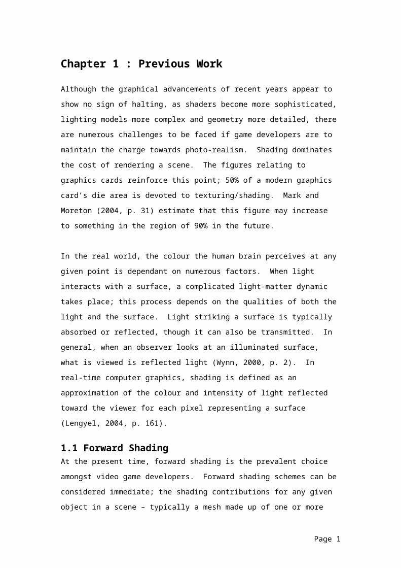
Figure 1 The ceiling mesh has been rendered with an ambient lighting contribution (MPML)

Figure 2 The ceiling mesh is re-rendered using an omni-directional light shader in conjunction with additive blending (MPML)

Each approach has notable disadvantages. The former approach results in a combinatorial explosion of shaders to accommodate all possible light configurations and does not integrate well with contemporary shadowing techniques. The latter approach results in the same initial setup transformations being repeated for every light influencing the object. For example, transformed vertex and normal values, normal map decompression, anisotropic texture filtering etc. may be required for each and every shading pass.

In addition these problems, the multiple-pass forward shading scheme also suffers from reduced batching efficiency. A batch is simply a draw call such as Direct3D’s DrawIndexedPrimitive (Wloka, 2003, p. 2). Since objects are being drawn multiple times, this increases the amount of required draw calls and state changes. Even with optimisations such as texture atlases and using a large vertex buffer for multiple objects, the increase in state changes and draw calls is largely unavoidable.

1.3 Deferred ShadingDeferred shading is simply the decoupling of the transformation of an object and the calculation of its shading contribution to the scene, hence

Page 2

the name deferred shading. Instead of transforming the object and immediately calculating the shading contribution to the scene, the object’s per-pixel attributes (such as position, diffuse, normal, gloss etc.) are written to an intermediate “fat” buffer (or G-Buffer) and stored for further use. The G-Buffer is typically comprised of a series of renderable textures. The application is then free to refer to the G-Buffer’s contents to calculate the contribution of each light to the scene during a separate lighting pass (Heargreaves & Harris, 2004, p. 12). Each light is additively blended into an accumulation buffer. Once all lights have been evaluated, the accumulation buffer can either be displayed to the user, or used as an input into further post processing shaders.

Page 3

Figure 3 Diffuse render target Figure 4 View space normal render target

Figure 5 View space position render target

Figure 6 Visualisation of omni-directional light source being additively blended into the light accumulation render target

The aim of the project is to comparatively evaluate deferred and forward shading with a view to characterising the strengths and deficiencies associated with each in the context of real-time computer games. This will be achieved by implementing each technique in sample applications which, in turn, tackle common problems found in real-time games. The performance and visual fidelity of each technique can then be compared for each particular situation. Just as importantly, by creating these applications it will provide an insight into the more conceptual and less

Page 4

readily graspable areas of batch management (the grouping of draw calls sharing common states), ease of use, compatibility with common effects (primarily shadow rendering) and so forth.

Put simply, the aim is to better understand the technical and conceptual strengths and weaknesses of deferred shading when contrasted with prevalent methods of forward shading.

1.4 Research QuestionWhen implementing deferred shading as a replacement for forward shading in real time computer games, what is a characterisation of the issues involved?

In answering the question, the research will focus on these areas:

Scene management, including how batching is organised. Rendering performance in a variety of common situations. Image fidelity. Ease of use Ease with which modern effects such as tangent space normal

mapping, shadow mapping, fog, HDR etc. were able to be added to the application (i.e. compatibility and extensibility).

The rationale for the selection of these issues for investigation is that they all have a significant impact on the development process or the quality of the finished game. If a technique is relatively simple to implement and extend, it aids developer efficiency. Likewise, the player of the game will expect good image quality and interactive frame-rates.

Chapter 2 : Organisation

In chapter 3, a review is conducted into the two primary forward shading rendering techniques. A review of previous work pertaining to deferred shading is also conducted. The various high level issues, advantages, disadvantages and so forth are discussed in addition to potential

Page 5

additional applications of deferred shading such as volumetric effects. Finally, the gaps in the existing literature are identified.

Chapter 4 contains the rationale for implementing various techniques related to both deferred and forward shading. It also includes the implementation details and a brief exposition of how the quantitative results will be collected and evaluated.

Chapter 5 presents the measurable results.

Chapter 6 evaluates the results and also critically analyses the less readily measurable aspects (such as ease of use and implementation, extensibility etc.)

Chapter 7 summarises the work, provides conclusions and suggestions for future work.

The appendices contain some additional details that were not felt to fit into the main report body, but the interested reader may find them to be of use.

Page 6

Chapter 3 : Previous Work

3.1 Deferred ShadingAlthough the use of deferred shading in real-time computer games is largely uncommon, the concept itself is almost two decades old. Deferred shading was first suggested by Deering et al. (Siggraph 1988) for use in offline rendering. In years gone by, deferred shading has been prohibitively expensive to implement on most platforms due to lacking performance and features, but it will become increasingly attractive as hardware progresses (Hargreaves, 2004).

Indeed, with the advent of Pixel Shader 2.0 class graphics cards, deferred shading has become a realistic proposition for use with PC games. Pixel Shader 2.0 compliant cards are able to render to multiple render targets simultaneously. The significance of this feature relates to the fact that the G-Buffer creation phase can be completed more efficiently (Thibieroz, 2003). Prior to Pixel Shader 2.0, each set of attributes stored in the G-Buffer would require a separate rendering pass; this made the technique largely unfeasible. At the present time, only a handful of games such as Red Storm’s “Ghost Recon Advanced Warfighter” have utilised deferred shading. Many commentators have struggled to reach a consensus regarding deferred shading’s worth or future; as Nvidia’s “6800 leagues” presentation states, “More research is needed!” (Hargreaves & Harris, 2004, p. 36).

Figure 7 Red Storm’s GRAW. Deferred shading in action.

Page 1

3.3 Forward ShadingHargreaves & Harris (2004) outline the primary considerations developers face when choosing a shading model. There are two primary methods utilised when shading scenes in currently available real-time games: Single pass, multiple light (SPML) and multiple pass, multiple light (MPML).

3.3.1 Single Pass, Multiple Light (SPML)SPML applies all lighting to the scene in a single shader which avoids the duplication of transforms associated with multiple passes. While this may seem attractive, the SPML shaders must be able to handle every single combination of lighting inputs. This typically results in a combinatory explosion of shader permutations, especially when multiple shading models are to be supported. SPML is also largely incompatible with modern shadowing techniques. Shadow volumes require a per-light stencil pass which is not possible if all lights are summed up in a single shader, whereas shadow mapping would require that all shadow maps be present in video memory prior to the lighting being evaluated. Finally SPML has a tendency to overflow shader length limitations (Heargreaves, 2004, p. 3).

3.3.2 Multiple Pass, Multiple Light (SPML)The alternative of MPML often requires several rendering passes to cumulatively shade an object. Each mesh influenced by N lights requires N rendering passes, and each pass is additively blended into an accumulation buffer

Page 2

Figure 8 id Software’s DoomIII. MPML forward shading in action.

When using traditional MPML forward shading schemes, the results of transforming vertices and calculating normals, parallax and other data cannot be stored for future reference. When an object is illuminated by multiple lights, this intermediate data is common to each pass, but must be recalculated and discarded each and every pass. When triangle meshes are comprised of several thousand vertices and refer to multiple texture maps (many of which require decompression and additional computation each time they are referenced), this extra computation soon becomes noticeable. In a scene with L lights and N objects, the worst case complexity is N * L rendering passes (Hargreaves, 2004, p. 4). While it is possible to perform visibility checks to cull unseen lights and geometry, such checks are always conservative. Such visibility schemes typically operate using coarse approximations such as bounding primitives (spheres, boxes, cones) which results in many pixels being needlessly evaluated.

In addition to these technical drawbacks, a modern MPML forward shading renderer also requires significant behind the scenes management. To minimise the shading costs, each light must be able to determine whether each visible object is in its area of influence. The process of sorting and submitting draw calls and state changes is not a trivial problem to solve, nor is it free in terms of CPU time. When a mesh must be re-rendered for each light influencing it, a growth in the number of required state changes and draw calls is inevitable. Games have multiple subsystems all competing for processor time so it is important that the renderer does not

Page 3

consume a large proportion of the game’s frame time, else the game may be CPU limited as a result (Wloka, 2003). Shishkovtsov (2005, p. 144) states that many games are CPU bound and techniques like deferred shading can potentially ease the load.

Even worse, overdraw (the action of drawing the same pixel more than once) is almost guaranteed to occur when forward shading is utilised. As shaders become ever more complex, pixels that are repeatedly filled represent a costly waste of resources. In scenes featuring significant overdraw, the fill rate of the graphics card is often a bottleneck (Latta, 2004, p.119).

In the past, these problems haven’t been hugely crippling as, regardless of the ingenuity of developers, fully dynamic lighting and shadowing simply wasn’t feasible using the hardware of that era. Games typically employed static, pre-computed lighting solutions such as light maps (Abrash, n.d.) and simplistic shadowing techniques such as planar shadows. However, ever since Doom III debuted with its fully dynamic, unified lighting model, developers have been working on ever-more sophisticated lighting schemes. As the number of dynamic lights increases, forward shading begins to look a little unwieldy, both in terms of batching and technical constraints.

3.4 Deferred ShadingAs previously mentioned, deferred shading is a large departure from the traditional forward shading schemes. The scene attributes (such as position, normals, diffuse etc.) are written to a “G-Buffer” that is typically comprised of an array of three or more render targets. Using hardware featuring pixel shader 2.0 or better, a G-Buffer comprised of four or fewer render targets can be populated in a single scene pass.

Page 4

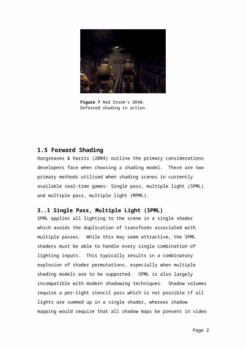
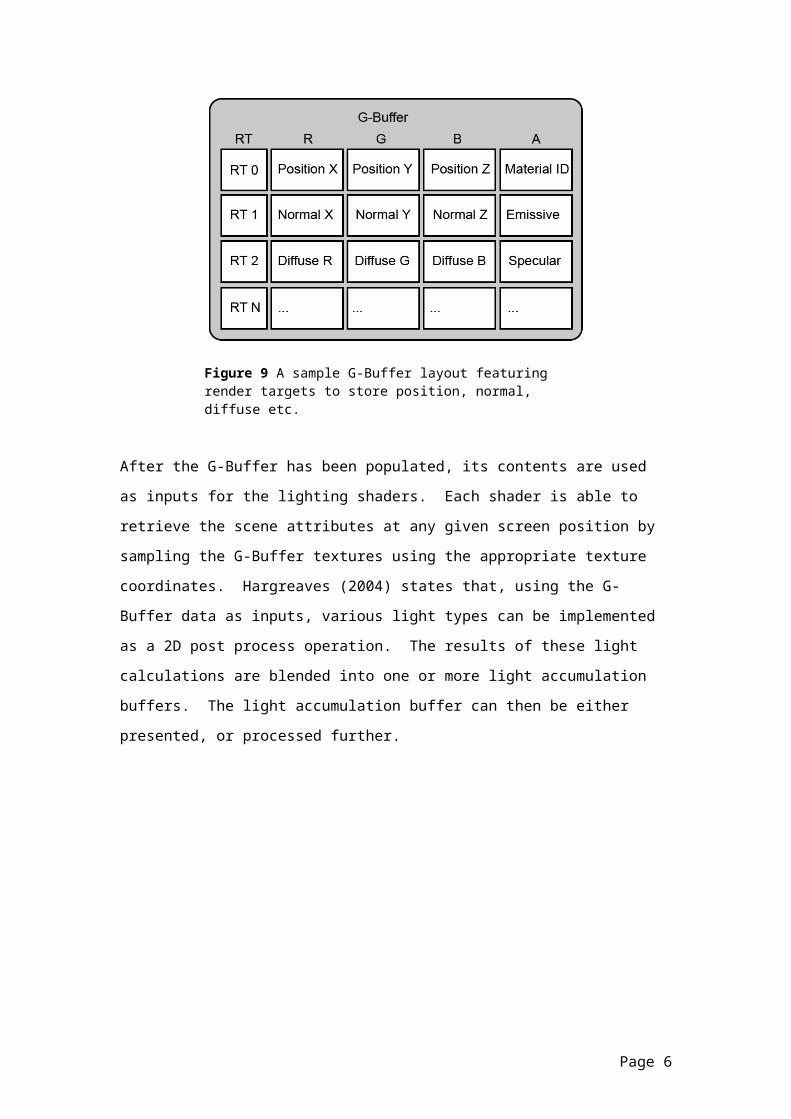
Figure 9 A sample G-Buffer layout featuring render targets to store position, normal, diffuse etc.

After the G-Buffer has been populated, its contents are used as inputs for the lighting shaders. Each shader is able to retrieve the scene attributes at any given screen position by sampling the G-Buffer textures using the appropriate texture coordinates. Hargreaves (2004) states that, using the G-Buffer data as inputs, various light types can be implemented as a 2D post process operation. The results of these light calculations are blended into one or more light accumulation buffers. The light accumulation buffer can then be either presented, or processed further.

Page 5

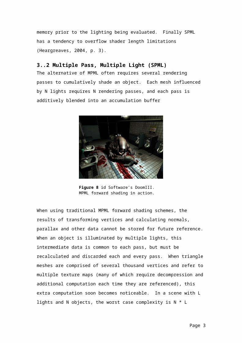
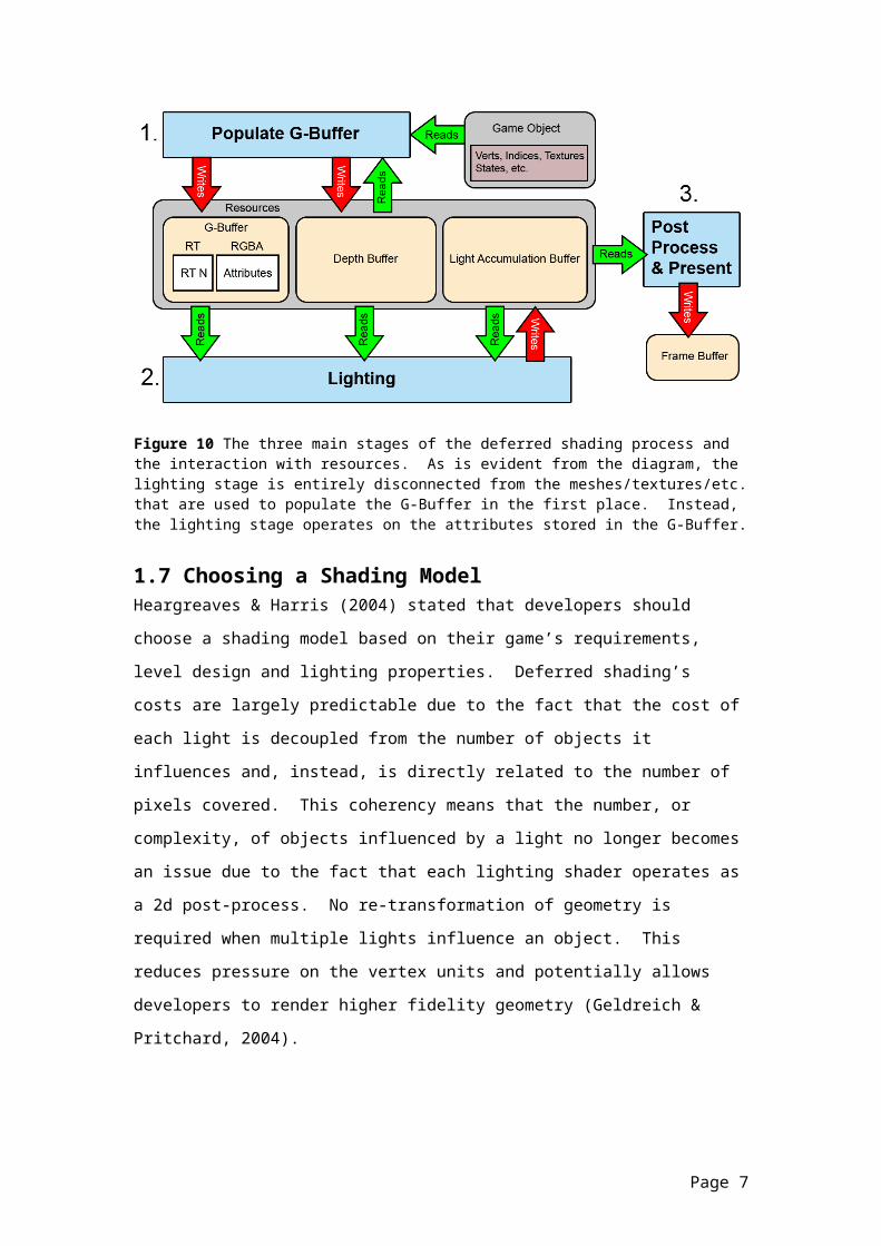
Figure 10 The three main stages of the deferred shading process and the interaction with resources. As is evident from the diagram, the lighting stage is entirely disconnected from the meshes/textures/etc. that are used to populate the G-Buffer in the first place. Instead, the lighting stage operates on the attributes stored in the G-Buffer.

3.5 Choosing a Shading ModelHeargreaves & Harris (2004) stated that developers should choose a shading model based on their game’s requirements, level design and lighting properties. Deferred shading’s costs are largely predictable due to the fact that the cost of each light is decoupled from the number of objects it influences and, instead, is directly related to the number of pixels covered. This coherency means that the number, or complexity, of objects influenced by a light no longer becomes an issue due to the fact that each lighting shader operates as a 2d post-process. No re-transformation of geometry is required when multiple lights influence an object. This reduces pressure on the vertex units and potentially allows developers to render higher fidelity geometry (Geldreich & Pritchard, 2004).

Furthermore, optimisations such as using projected light volumes can also be used. Hargreaves (2004, p.21) suggests implementing a masking algorithm similar to that of shadow stencil volumes. The resultant stencil mask contains only the pixels where the light volume intersects scene geometry meaning the number of pixels being evaluated for lighting is kept to a bare minimum.

Page 6

Rather than minimising the number and complexity of objects, the main consideration in maintaining performance is minimising the number of pixels being lit. In short, it operates in a fashion that is markedly different to forward shading and, depending on a game’s design, may free the developer from various design constraints. There are caveats, though. If multiple overlapping lights occupy much of screen, the shading complexity will inevitably be high. Combined with the cost of the G-Buffer setup, it may offset any gains and prove to be slower than forward shading (Hargreaves & Harris, 2004, p. 33). Due to the use of MRTs, deferred shading is inherently unable to take advantage of certain types of anti-aliasing, too.

Finally, the attributes in the G-Buffer can also be used as inputs to various special effects. This approach has been adopted in cutting edge game engines such as Epic’s Unreal Engine 3 and Crytek’s CryEngine. While the lighting and/or shading is not necessarily deferred, a G-Buffer pass (sometimes storing depth is all that is required) can be utilised to enhance special effects such as realistic fog, smoke and clouds, bodies of water, shadows, soft particles and so on (Wenzel, 2006).

While much has been written about the high level issues, gaps exist in the existing literature. Specifically, the existing recommendations are very general and a more expansive characterisation would be beneficial to developers when deciding whether a particular game type would be better served by a forward or deferred shading architecture.

Page 7

Chapter 4 : Methods

4.1 Chapter StructureThis chapter is divided into four main parts. The first details the common functionality inherent to both the deferred and forward shading renderers. The second describes the implementation of the deferred shading renderer. The third describes the implementation of the forward shading renderer. The fourth deals with the scene types and criteria used when performing the comparative tests.

Each subsection is further divided into an exposition of the method, the relevance to the work being carried out, considerations that were made and any specific implementation details that should be known.

To provide a meaningful comparison of forward and deferred shading schemes, it was necessary to implement both techniques. As stated in the literature review, single pass multiple light forward shading does not integrate well with modern shadowing techniques. As a result, multiple pass multiple light shading was the most fitting option when implementing a forward shading model. This choice made it simpler to directly compare and evaluate the forward and deferred shading schemes, as both renders were able to support the same features.

The artefact was written using C++, the Direct3D API and the High Level Shader Language (HLSL). Direct3D and HLSL were chosen due to their support for Effect files. Effect files encapsulate shaders and states, making it simpler to design, create and manage a project of this kind. The Phong lighting model (Phong, 1975, p. 311-317) is used for all lighting calculations. The program is intended for NVIDIA Geforce 6 series graphics cards or above. Due to the use of NVIDIA depth stencil surfaces, a non-NVIDIA GPU may fail to run the application. Certain results (such as DrawPrimitive counts and the time spent per stage of the rendering pipeline) were obtained using NVIDIA’s NVPerfHUD analysis tool. Additional tests were also performed to evaluate the performance of optimisation techniques.

Page 8

Since large parts of both the deferred and forward shading renderers required common functionality (e.g. frustum culling of meshes & lights, shadow set generation and shadow map rendering, visualisation of bounding meshes etc.), the renderers inherit from a single base class, ID3DRenderer.

It should be noted that in certain images captured from the artefact using NVPerfHUD, an orange wireframe denotes the last rendered primitive.

4.2 Common Functionality

4.3.1 Set RepresentationRather than building explicit lists to represent set membership, sets are represented using an indirect method: flags. A flag is simply a way of marking an entity as being a member or a non-member of a particular set. These flags are stored as member variables (typically bools or unsigned integers) and can be tested to determine set membership.

4.3.2 View Frustum Culling & Intersection TestsTo reduce the number of redundant state changes and draw calls, a handful of standard visibility tests are used. These checks include frustum culling of bounding spheres and axially aligned bounding boxes (NVIDIA, 2003) & (Glassner, 1990 p. 335). Prior to rendering the scene, the objects and lights contained in the scene file are tested against the view frustum. Visible objects or lights (a visible object is one whose bounding volume passes the view frustum intersection test) are placed in the visible set, V. Rather than building an explicit list, the set is represented using a simple Boolean flag stored as a member variable of each scene object.

Additionally, various standard intersection tests were implemented. Although certain tests are used solely by the forward shading renderer, it was felt to be more natural to implement these features in a wholly separate class (bounding.h/.cpp) given that they are utility functions and unrelated to the renderer itself.

4.3.3 Primitive SortingTo evaluate the way in which deferred and forward shading affects batching schemes, it is necessary to form a rendering queue that is

Page 9

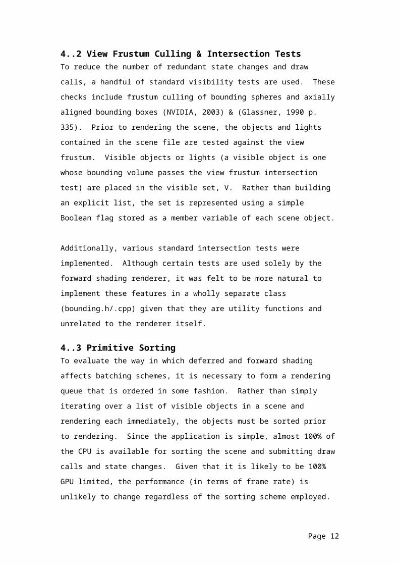
ordered in some fashion. Rather than simply iterating over a list of visible objects in a scene and rendering each immediately, the objects must be sorted prior to rendering. Since the application is simple, almost 100% of the CPU is available for sorting the scene and submitting draw calls and state changes. Given that it is likely to be 100% GPU limited, the performance (in terms of frame rate) is unlikely to change regardless of the sorting scheme employed. As a result, the number of state changes and draw calls is the metric by which the success of the method will be evaluated. In a full game, AI, collision detection, physics etc. all compete for resources, so it is important that the state changes are minimised.

The application uses a scheme whereby the primitives are sorted by diffuse texture. Although this is a coarse approximation of minimising state changes – as much more sophisticated schemes exist and it is difficult to determine the absolute ‘best’ criteria by which to sort (Zerbst, 2004, p.286) – it introduces a basic ordering of draw calls. This is necessary when attempting to determine whether each renderer introduces additional state changes and draw primitive calls.

To sort by texture, the rendering queue is grouped by textures in state ‘buckets’. A bucket is simply a list of one or more triangle lists sharing a common render state. In this case, the diffuse texture is used as the key.

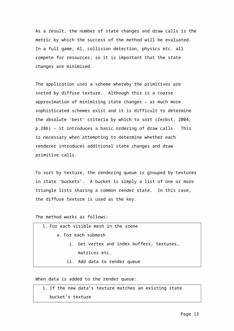
The method works as follows:1. For each visible mesh in the scene

a. For each submeshi. Get vertex and index buffers, textures, matrices etc.ii. Add data to render queue

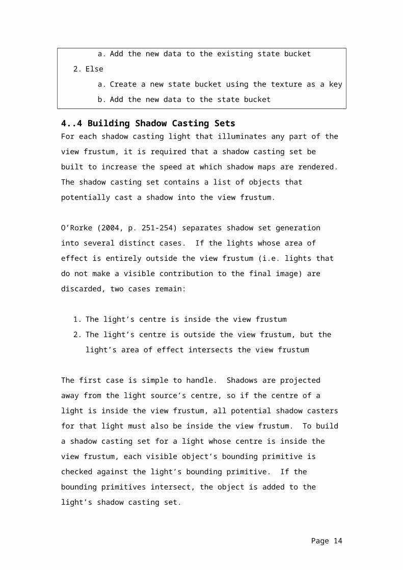
When data is added to the render queue:1. If the new data’s texture matches an existing state bucket’s texture

a. Add the new data to the existing state bucket2. Else

a. Create a new state bucket using the texture as a keyb. Add the new data to the state bucket

Page 10

4.3.4 Building Shadow Casting SetsFor each shadow casting light that illuminates any part of the view frustum, it is required that a shadow casting set be built to increase the speed at which shadow maps are rendered. The shadow casting set contains a list of objects that potentially cast a shadow into the view frustum.

O’Rorke (2004, p. 251-254) separates shadow set generation into several distinct cases. If the lights whose area of effect is entirely outside the view frustum (i.e. lights that do not make a visible contribution to the final image) are discarded, two cases remain:

1. The light’s centre is inside the view frustum2. The light’s centre is outside the view frustum, but the light’s area of

effect intersects the view frustum

The first case is simple to handle. Shadows are projected away from the light source’s centre, so if the centre of a light is inside the view frustum, all potential shadow casters for that light must also be inside the view frustum. To build a shadow casting set for a light whose centre is inside the view frustum, each visible object’s bounding primitive is checked against the light’s bounding primitive. If the bounding primitives intersect, the object is added to the light’s shadow casting set.

The second case is much more difficult to solve. As per O’Rorke’s method, an attempt was made to construct a convex bounding hull that represents the smallest hull surrounding the view frustum and light. Due to time constraints this work was not fully completed. To generate a shadow casting set for this case, a brute force method was implemented. All meshes are added to the shadow casting set. Due to the fact that the application’s scenes do not contain hundreds of meshes and the shadow set rendering is common to both renderers, this does not represent a large problem.

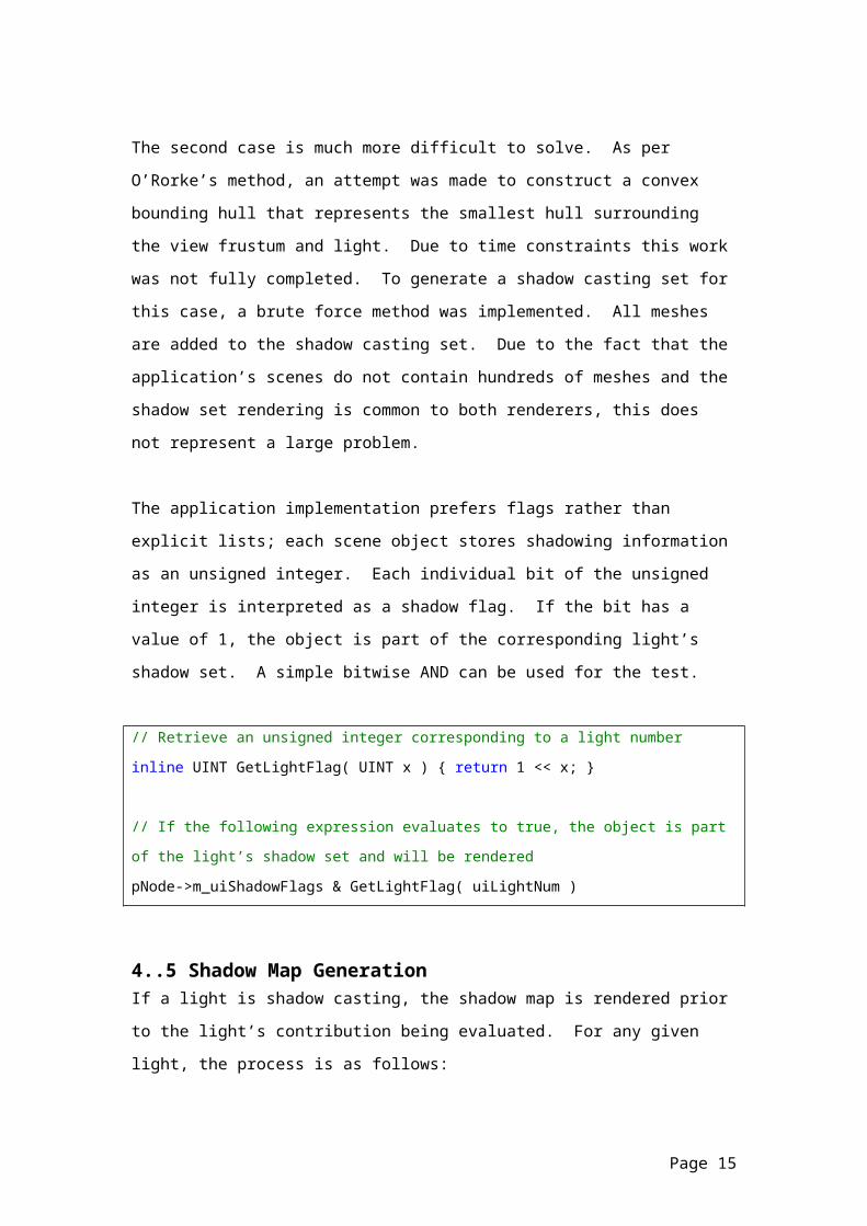
The application implementation prefers flags rather than explicit lists; each scene object stores shadowing information as an unsigned integer.

Page 11

Each individual bit of the unsigned integer is interpreted as a shadow flag. If the bit has a value of 1, the object is part of the corresponding light’s shadow set. A simple bitwise AND can be used for the test.

// Retrieve an unsigned integer corresponding to a light number

inline UINT GetLightFlag( UINT x ) { return 1 << x; }

// If the following expression evaluates to true, the object is part

of the light’s shadow set and will be rendered

pNode->m_uiShadowFlags & GetLightFlag( uiLightNum )

4.3.5 Shadow Map GenerationIf a light is shadow casting, the shadow map is rendered prior to the light’s contribution being evaluated. For any given light, the process is as follows:

1. Store the old render target2. Bind shadow map depth stencil surface as render target3. For each object in the light’s shadow casting set

a. Calculate a matrix to take the mesh from object to light projection space

b. Transform the mesh by the matrix4. Unbind the shadow map as the render target5. Rebind the old RT

4.3 Deferred Shading

4.3.6 G-Buffer FormatHargreaves & Harris (2004) and Shishkovtsov (2005) both recommend the use of 64-bit floating point A16R16G16B16F textures on modern GPUs.

The G-Buffer layout that was decided upon is as follows:

Page 12

Figure 11 Application G-Buffer format.

The position and normal vectors are stored in view space (a.k.a. camera or eye space). This is a convenient choice, as no unpacking or data manipulation is required; the positions and normals can be used in the majority of common lighting calculations without any modification. Again, this decision was made on the recommendation of the aforementioned authors.

According to Hargreaves & Harris (2004, p. 38), the G-Buffer render targets must be allocated first to ensure they are placed in the fastest graphics card RAM and, when using a NVIDIA Geforce 6 series card, due to a performance cliff when writing to more than three render targets, it is advisable to restrict the number of render targets to three or fewer. This obviously limits the number of attributes that can be written to the G-Buffer which, in turn, limits the amount of inputs available for the lighting calculations.

4.3.7 G-Buffer PassOne of the most important, if not the most important, stages of deferred shading is the process of populating the G-Buffer with the per-pixel scene attributes. In addition to filling the G-Buffer, by enabling depth reads & writes, the depth buffer can also be filled simultaneously. The process of filling the G-Buffer is as follows:

1. For (each mesh)a. Set states (vertex buffer, index buffer, textures)b. Render mesh, outputting attributes to G-Buffer

Page 13

The G-Buffer effect’s vertex shader performs a series of transformations to calculate the required attributes. A quirk of the deferred shading algorithm is that two positions must be calculated for each vertex. The first position is the standard clip space co-ordinate (the transformed vertex v’ = v * World * View * Projection). Although this position is neither stored nor referenced, it is used to fill the depth buffer. The second position is the view space co-ordinate (vs’ = v * World * View). Additionally, the view space normal vector (n’ = n * World * View) and texture co-ordinates are also calculated.

In the corresponding pixel shader, the interpolated view space position and normal vectors are written directly to the position and normal render targets respectively. Since the application uses a 64 bit floating point format, the attributes can be written without manipulation or range compression. An emissive term is stored in the normal render target’s alpha channel. Finally, the diffuse texture colour is written to the diffuse render target. To indicate the reflectivity of each pixel, a specular (gloss) term is stored in the diffuse render target’s alpha channel.

4.3.8 Tangent Space Normal MappingWhile the above solution is perfectly acceptable for many uses, it is missing support for the ubiquitous rendering technique of modern times: Tangent space normal mapping. The traditional method of performing tangent space normal mapping requires performing lighting calculations in tangent space. As the tangent space transformation matrix is formed using the tangent, bitangent and normal vectors of each triangle’s vertices, it is clearly not possible to perform the lighting calculations in tangent space as the per-triangle data is no longer available. Instead, the opposite approach must be taken: when filling the G-Buffer, the tangent space normals are transformed to match the format of the G-Buffer normals; since the G-Buffer’s normals are stored in view space, this means transforming to view space.

It should be noted that while this requires a per-pixel matrix multiplication (as opposed to per vertex with forward shading), the normals do not require decompression & recalculation in future shading passes.

Page 14

The familiar tangent space calculation is as follows:

float3x3 TBN = float3x3( Input.Tangent, Input.Binormal, Input.Normal)

float tangentSpacePosition = mul( TBN, Input.Position)

Multiplying a transposed object space row vector v by the TBN matrix (giving TBN * vT) produces a transformed vector v’ in tangent space. As the opposite is required, the tangent space normal vectors must be first transformed to object space. Since the TBN matrix can be treated as being orthogonal, the fact that the inverse of an orthogonal matrix is its transpose can be exploited. Multiplying a tangent space row vector t by the TBN matrix produces a transformed vector t’ in object space.

Taking it a step further, it is possible to concatenate an additional matrix multiplication in the vertex shader to obtain a matrix that will transform a tangent space normal to view space. This matrix is then split into its constituent row vectors and passed to the pixel shader as a series of 3D texture co-ordinates.

// Vertex ShadermatTBN = float3x3( Input.Tangent, Input.Binormal, Input.Normal );matTangentToViewSpace = mul( matTBN, matWorldView );

Out.TangentToView0 = matTangentToViewSpace[0];Out.TangentToView1 = matTangentToViewSpace[1];Out.TangentToView2 = matTangentToViewSpace[2];

Finally, the corresponding pixel shader re-assembles the tangent to view space matrix and uses it to transform the tangent space normal into view space.

// Pixel Shaderhalf4 normalMapIn = tex2D( normalMap, Input.TexCoords );half3 tangentSpaceNormal = normalMapIn.xyz * 2 - 1;

float3x3 matTangentToViewSpace = float3x3( Input.TangentToView0, Input.TangentToView1, Input.TangentToView2 );

half3 viewNormal = mul( tangentSpaceNormal, matTangentToViewSpace );

Page 15

4.3.9 Accessing the G-BufferOnce the G-Buffer has been populated, its contents can be used as inputs for lighting calculations. Reading the G-Buffer’s contents is a simple operation, but there is a pitfall to be aware of; Direct3D9’s texel sampling rules aren’t quite what one may expect. Using a raw texture co-ordinate will yield poor results as Direct3D does not directly map texels to pixels.

The Microsoft Direct3D documentation (Microsoft, n.d.) states:

“…Pixels and texels are actually points, not solid blocks. Screen space originates at the top-left pixel, but texture coordinates originate at the top-left corner of the texture's grid….”

It is relatively simple to correct the texture co-ordinates to account for this discrepancy by adding a constant to the existing texture co-ordinates.// account for DirectX's texel center standard:float u_adjust = 0.5f / width;float v_adjust = 0.5f / height;

Figure 12 No texture co-ordinate adjustment. Strong aliasing is evident.

Figure 13 Adjusted texture co-ordinates. No discernable image degradation.

4.3.10 Ambient lighting & Emissive TermAmbient lighting is uniformly applied to all objects in a scene and is written directly to the light accumulation buffer, serving as a base colour. The easiest way to implement such an effect with deferred shading is to

Page 16

render a full-screen quad, outputting the diffuse colour multiplied by the ambient term. If an emissive term is present, the corresponding pixel’s diffuse colour is modulated by this value. This ensures that light will always appear to be emanating from physical light sources (bulbs, tubes, fittings etc) or other objects that require such an effect.

Figure 14 Diffuse Figure 15 Emissive term Figure 16 Ambient & emissive

4.3.11 Shadow mappingTraditionally, shadow mapping works by performing a per-vertex transformation taking a mesh’s vertices from object to light projection space. The interpolated light projection space position is then sent to the pixel shader. The depths can then be compared and the shadowing term calculated. However, much like tangent space normal mapping, the algorithm requires a change as the vertices are no longer available when using the G-Buffer contents. Instead, the position of each lit pixel in the G-Buffer must be transformed into light projection space. Since the pixel positions are stored in view space, this involves:

1. Going first from view to world space using the inverse view matrix2. Then from world to light projection space.

Once in light projection space, the g-buffer pixel’s depth can be compared with the shadow map depth, yielding the shadowing term. Aside from this alteration, shadow mapping integrates very well with deferred shading.

Page 17

Shadow mapping was implemented for spot and directional lights. The rendering process for a shadow casting light is as follows:

1. Set the shadow map render target as a texture for the lighting shader

2. Calculate a matrix to transform a view space co-ordinate into the light’s view projection space. (v’ = v * inverse view * light view * light projection)

3. In the lighting pixel shader, read the pixel’s view space position from the G-Buffer

4. Transform the view space position into light view projection space.5. Use the depth of the pixel’s transformed position to calculate the

shadowing term 6. Modulate the colour by the shadowing term

4.3.12 Directional lightsLike ambient lighting, directional lights are rendered using a full-screen quad. The Phong lighting equation is calculated at each pixel. Since each light is adding further lighting contribution to an existing buffer, additive blending is used. The normal, diffuse and specular terms are retrieved from the G-Buffer and plugged into the standard Phong lighting equation.

Page 18

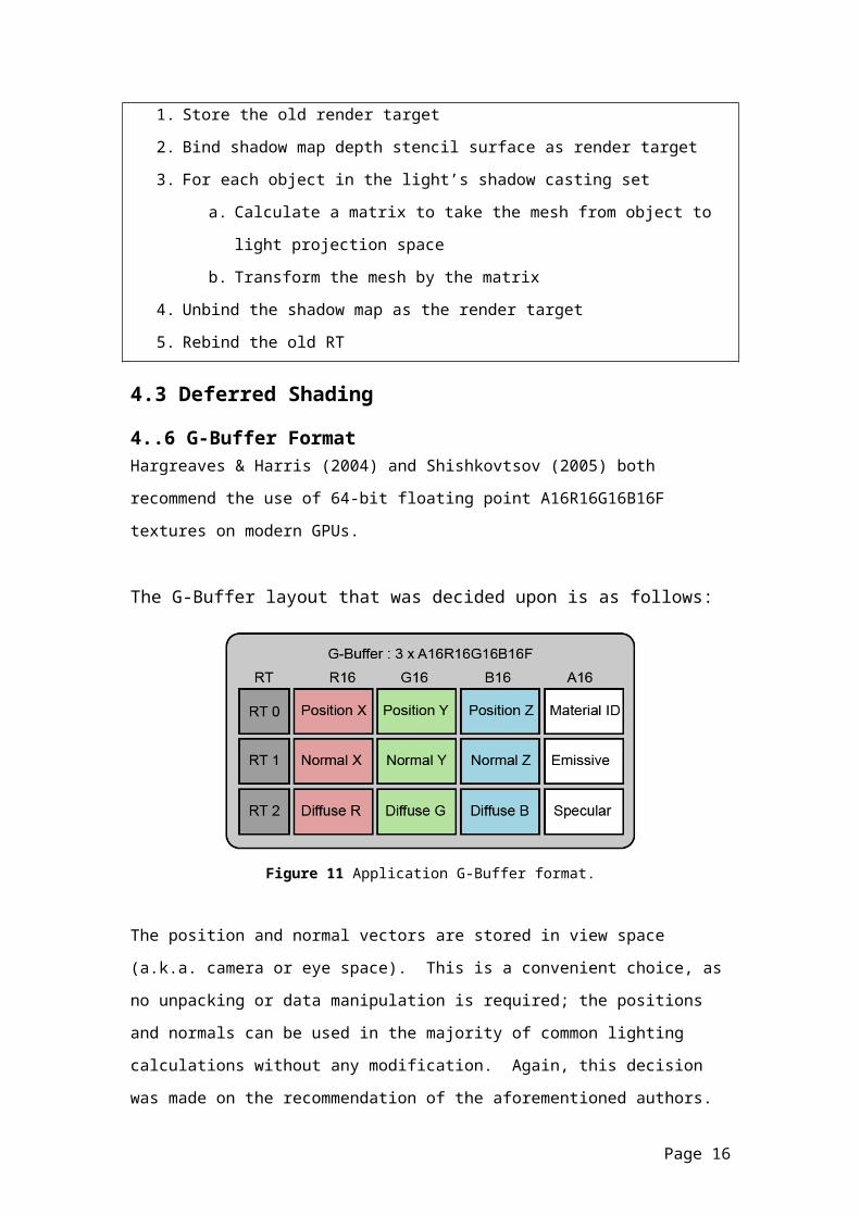
Figure 17 Canyon scene. Contents of the light accumulation buffer prior to directional lighting.

Figure 18 Canyon scene. Contents of the light accumulation buffer after a directional light contribution.

4.3.13 Localised LightingLocalised lighting, such as omni-directional and spot lights, can be implemented using a number of different methods. A naïve approach would be to render a full-screen quad for each and every light source. This would produce the correct lighting results, but would be hugely wasteful in terms of performance, as every pixel in the scene would be evaluated. For an application featuring a resolution of R pixels and a scene with N lights, the shading complexity would be O(N * R) (Hargreaves & Harris, 2004, p. 34).

There are numerous optimisation schemes available such as scissor rectangles (Policarpo & Fonseca, 2005, p.18), but while these offer a performance increase, they do not eliminate all wasted shading. Instead, the GPU is utilised to project into screen space a light hull representing any given light’s area of influence. For example, for an omni-directional light source of maximum range R and position P, a sphere can be created whose centre is located at P and whose radius is equal to R. Once transformed and rasterised in the usual fashion, it exactly bounds the light’s area of influence.

This method on its own only better approximates a light’s screen space region. It cannot differentiate between pixels intersecting a light hull (illuminated) and pixels that are occluded or ‘floating’ (not illuminated).

Page 19

To make this distinction, a further enhancement must be made. Hargreaves (2004, p.21) suggests employing the stencil buffer in a fashion similar to that of the way it is used to render shadow volumes.

The stencil buffer can be employed to create a sophisticated mask. In this case, this mask indicates which pixels require the lighting calculations. This technique is expanded upon (Hargreaves & Harris, 2004, p. 16) and the details are as follows:

1. Render light volumes without colour writesa. Set depth func = less; b. Stencil func = alwaysc. Stencil Z-Fail = replace with Xd. All other stencil ops = keep

2. Render with light shadera. Depth func = alwaysb. Stencil func = equalc. All ops = keepd. Stencil ref = X

The intended result of the above method is that only pixels where lights intersect scene geometry will pass the stencil test during the second pass. However, a problem was identified with the explanation given. To understand the problem it is necessary to consider the three possible outcomes when rendering a light hull:

1. The light hull is fully in front of the scene geometry2. The light hull is enclosing scene geometry3. The light hull is fully behind scene geometry

The algorithm works correctly when the pixel is in front (passes depth test, stencil bit not set) and inside the light hull (back faces of lighting hull will fail depth test, stencil bit set to reference value), but when an object exists between the viewer and the light volume, the depth test will fail and the stencil bit will be set to the reference value. This means the pixel will pass the stencil test for the lighting pass. This is not the desired

Page 20

behaviour! Visually, the image will be correct (as the pixels evaluated have a position that will result in a lighting contribution of 0), but it will not be optimal in terms of performance.

Solving the problem is straightforward. As Hargreaves stated, the problem is akin to one faced when rendering shadow volumes. To give a very brief exposition of the technique, shadow volume rendering works by rendering a 3D representation of a shadow’s area of influence (Lengyel, 2002). This is done separately for both front and back faces. If the front or back faces of the shadow hull pass/fail the depth test, the stencil value is either incremented or decremented (the details depend on whether a depth pass or depth fail algorithm is being used). This is essentially a graphical way to count the number of times the ray from the camera to a point crosses a shadow boundary (as to know whether a point is in shadow, it must be know whether a ray from the camera to the point enters and then fails to exit a shadow hull).

Much the same thing can be done to count the number of times a ray from the camera crosses a light boundary. This was achieved as follows (“Hellraizer”, 2007):

1. Clear stencil value to 1.2. Render front faces of light volume to stencil buffer

a. Depth func = lessb. Stencil Z fail = increase

3. Render back faces of light volume to stencil buffera. Depth func = lessb. Stencil Z fail = decrease

4. Render back faces of light hull using light shadera. Stencil reference value = 0

Page 21

The algorithm is best explained with the aid of a diagram:

Figure 19 Creating a stencil buffer mask. The camera is represented by C, the figures represent scene geometry and the yellow circle is the hull of an omni-directional light source. Pixels with a stencil value of 0 are inside the light hull.

The three lines represent rays emanating from the camera position C, each corresponding to a pixel on the camera near plane. Each ray represents one of the three cases previously mentioned (the light volume is either in front of, intersecting or behind the scene geometry). For rays that enter but do not exit a light volume, the stencil value will equal 0 at that particular pixel. All other cases will result in a non-zero value.

Finally, the two stencil passes (steps 2 and 3) can be combined into a single stencil pass if a graphics card with double-sided stencil support is available. The final technique requires a total of two passes.

Page 22

Figure 20 (Hargreaves, 2004). Light volume stencil optimisation. The spotlight cone mesh is the black wireframe. The bright pixels inside the spotlight cone represent areas where the spot lighting shader will be executed. Notice the ‘floating’ and ‘buried’ regions do not pass the stencil test, reducing wasted shading.

Now that the area that requires lighting calculations has been accurately determined, for each pixel passing the stencil test, the scene attributes from the G-Buffer must be retrieved. Unlike when rendering a full screen quad (whose texture co-ordinates already range from 0 to 1 and cover the entire screen) the texture co-ordinates have to be manually calculated. The standard method of calculating the texture co-ordinates involves, for each vertex of the light hull, calculating homogeneous clip space co-ordinate and then scaling and biasing to yield a result in the range 0 to 1.

A simpler solution exists for graphics cards with Shader Model 3.0 or better. The position register (vPos) contains the screen x and y co-ordinates of the pixel currently being processed (Thiberioz, 2003, p. 257). Dividing by the viewport width and height obtains co-ordinates ranging from 0 to 1 and, finally, the co-ordinates are corrected to account for Direct3D’s texel to pixel mapping. Using these texture co-ordinate values in conjunction with texture lookups, the G-Buffer attributes for any given pixel can be retrieved.

// Calculating and correcting the G-Buffer texture co-ordinates

Page 23

float2 coords = Input.vPos.xy / g_fScreenSize.xy;coords += g_fUVAdjust;

4.3.14 Omni-directional LightsNow that a robust means of rendering light volumes has been created, omni-directional lighting is trivial to implement. On initialising the application, a sphere mesh with radius 1 is created. When a light volume is to be rendered, a world matrix is created representing the light’s scale (where the scale is the light’s maximum range) and translation in the world. The standard Phong equation is then evaluated for each lit pixel and the value is additively blended with the contents of the light accumulation buffer.

4.3.15 SpotlightsCreating a physical representation of a spotlight isn’t as simple. The spotlight hull must be constructed on a per light basis and in a form where it can easily be transformed by a rotation matrix (see appendix).

Once the cone has been created, it can be rotated and translated to match the spotlight’s position and orientation in the world. The cone is rendered and, finally, the standard Phong spotlight lighting equation is applied for each lit pixel.

4.3.16 SkyboxWriting to the G-Buffer involves calculating various attributes, but in the skybox’s case, these attributes are redundant. When rendering a skybox, the skybox’s position, normals and specular term aren’t required because it is unlit and assumed to be positioned infinitely far away from the camera. Instead, the skybox diffuse colour is written to the light accumulation buffer once all lighting calculations have been performed, but before post-processing occurs. This bypasses the G-Buffer entirely, saves bandwidth, fill-rate and processing costs (Hargreaves & Harris, 2004, p. 38).

The most common method of rendering a skybox is, upon starting the rendering of the frame, to simply disable depth writes and render the skybox. This method cannot be employed as the skybox must be

Page 24

rendered last. To accurately render the skybox last, an elegant vertex shader trick is employed (Thibieroz, 2006, p. 17).

In the skybox vertex shader:1. The clip space co-ordinate is calculated as per usual2. The z component of the transformed vertex is copied into the w

component3. Once the post-projective divide occurs, the final depth of each

skybox pixel will equate to ~1.0f (as if w = z, then z/z = ~1.0f)

Since the depth buffer contains a depth value of 1.0f on being cleared, it is obvious that, after rendering the scene geometry, any pixel with an untouched depth value (equal to 1.0f) is not occluded, so the skybox must be visible. Due to rounding errors, the depth test must be set to less or equal to avoid “z-fighting” artefacts.

Figure 21 Light accumulation buffer after the lighting has been fully calculated

Figure 22 Light accumulation buffer after the skybox has been rendered. Only pixels with a depth value of ~1.0f are filled.

4.3.17 Post Processing & Effects (Extensibility)To determine whether deferred shading’s markedly different method of rendering comes at the cost of extensibility, some additional effects were implemented.

Page 25

HDR was implemented as per the standard single path method found in the NVIDIA SDK HDR FP16x2 sample application (NVIDIA, 2003). The HDR algorithm works by using the light accumulation buffer as an input. It uses vertex texture fetch, anisotropic decimation and sRGB gamma correction. Since the light accumulation buffer was already a floating point format, extending the application to incorporate HDR was trivial. It should be noted that there is a bug in the application’s HDR calculations that results in the exposure being too high, but this is present for both the forward and deferred shading renderers. It is a shader bug rather than a problem with either renderer.

Finally, to determine whether the g-buffer’s position render target could effectively be used as input into image space post-processing effects, fog was implemented. The fog is added with no knowledge of the underlying geometry; it operates by reading the G-Buffer’s per-pixel depth (the z component of each position vector) and plugging it into a modified linear fog equation. Due to time constraints the fog effect is rather basic.

4.4 Forward Shading

4.3.18 Light and Illumination SetsOne of the major challenges of creating a forward shading renderer lies in being able to minimise the number of lighting passes. As previously mentioned, the worst case scenario for a scene containing N objects and L lights is N * L rendering passes. In the majority of cases, the number of passes can be significantly reduced by building an illumination set. An illumination set is defined as the intersection of the visible (V) and light sets (L) (O’Rorke, 2004). V is already known. For each light, L is the set containing all scene objects inside the light’s area of influence. Unless an object is both visible and lit by the light being considered, it is omitted from that light’s illumination set.

The final method is as follows:1. For each light that passes the frustum culling test

a. For each object that passes the frustum culling test (V)i. If object and light bounding volumes intersect (L)

1. Flag object as being lit by the light (V n L)

Page 26

While this requires additional computation and increases the complexity of the rendering process, if the application already possesses features to create shadow casting sets, much of the functionality is shared.

4.3.19 Depth, Ambient & EmissiveThe forward shading renderer’s first act is to fill the depth buffer and calculate the ambient & emissive term. Although it may be beneficial to do a dedicated depth pass with colour writes disabled, none of the shaders used in the application are particularly complicated. As such, all three values are calculated in a single pass.

If an emissive texture is present, the diffuse texture colour is multiplied by the emissive term. If no emissive texture is present, the diffuse texture colour is multiplied by the ambient colour.

4.3.20 Further lightingOnce the scene depth is stored and the light accumulation buffer has the ambient & emissive values present, additional lighting information can be added. To add further lighting contributions, the visible lights are iterated over and, using the appropriate light shader, all objects visible to that light are rendered. The depth test is set to equal, meaning only visible pixels receive further shading during this stage.

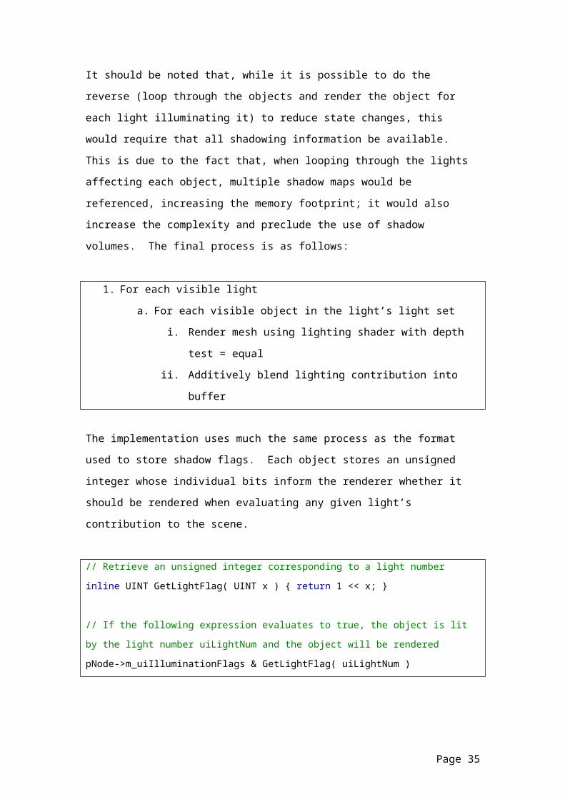
It should be noted that, while it is possible to do the reverse (loop through the objects and render the object for each light illuminating it) to reduce state changes, this would require that all shadowing information be available. This is due to the fact that, when looping through the lights affecting each object, multiple shadow maps would be referenced, increasing the memory footprint; it would also increase the complexity and preclude the use of shadow volumes. The final process is as follows:

1. For each visible light a. For each visible object in the light’s light set

i. Render mesh using lighting shader with depth test = equal

ii. Additively blend lighting contribution into buffer

Page 27

The implementation uses much the same process as the format used to store shadow flags. Each object stores an unsigned integer whose individual bits inform the renderer whether it should be rendered when evaluating any given light’s contribution to the scene.

// Retrieve an unsigned integer corresponding to a light number

inline UINT GetLightFlag( UINT x ) { return 1 << x; }

// If the following expression evaluates to true, the object is lit

by the light number uiLightNum and the object will be rendered

pNode->m_uiIlluminationFlags & GetLightFlag( uiLightNum )

Excluding the ambient lighting shader, each light shader includes the standard implementation of tangent space normal mapping.

4.3.21 Shadow mappingThe shadow mapping algorithm is straightforward. When rendering objects for use with a shadow casting light source, in addition to calculating the standard clip space position of each model vertex, the light projection space position is also calculated. The light projection space position is used to look up the shadow map. NVIDIA hardware shadow mapping automatically performs the depth comparison and returns the shadowing term. Finally, light value is modulated by the shadowing term.

The process is as follows:1. Set the shadow map render target as a texture for the lighting

shader2. Calculate a matrix to transform an object space co-ordinates into

the light’s view projection space. (v’ = v * world * light view * light projection)

3. When rendering geometry, in the vertex shader:a. Calculating the usual clip space co-ordinates & texture co-

ordinatesb. Also calculate the position in light projection space (as per

step 2)4. In the pixel shader:

Page 28

a. Use the linearly interpolated light projection space co-ordinate to look up the shadow map and retrieve the shadowing term.

b. Modulate the colour by the shadowing term

4.3.22 Directional LightsDirectional lights are treated as being global – all visible meshes in the scene are illuminated by a directional light and so illumination sets are not required. To calculate the contribution of directional light sources, each visible object in the scene is rendered using the Phong directional light shader and the result is additively blended into the light accumulation buffer.

4.3.23 Localised LightingThe remaining lights aren’t global in their nature. As such, to minimise the number of required rendering passes, the illumination sets are utilised.

4.3.24 Omni-directional LightsThe standard process is followed. For each light, each object in that light’s illumination set is rendered using the omni-directional light shader and the result is additively blended into the light accumulation buffer.

4.3.25 SpotlightsAgain, the standard process is followed. For each light, each illuminated object is rendered using the spotlight shader and the results are blended into the light accumulation buffer.

4.3.26 Post Processing & EffectsTo enable post-processing effects such as HDR, the light accumulation must be performed using an auxiliary buffer rather than the frame buffer. This auxiliary buffer is then used as an input into the post-processing effects.

4.5 Measuring PerformanceThere are various conceptual issues involved which cannot be readily measured in the form of figures (such as ease of use). Since there are no quantitative results in these areas, these areas are explored in the discussion/analysis section.

Page 29

Things that can be measured, such as the time spent rendering each frame (and the time spent during the various stages of the rendering pipeline) are collected using NVPerfHUD. The application was run several times at different resolutions to determine how resolution affects the performance at various stages of the pipeline, too.

The performance related to the number and screen space coverage of lights was tested by measuring the time spent rendering each frame with a handful of light configurations. Previous studies suggest that deferred shading is almost entirely fillrate bound, so the screen space coverage and overlapping of lights should dictate the performance.

A further test was performed to count the number of draw calls in the interior scene when shadows were disabled. This gives the absolute number of draw calls that directly relate to shading as opposed to shading and creating shadow maps.

Additionally, the image fidelity of each renderer is directly compared by taking screenshots in identical positions.

4.6 ScenesThe scenes are loaded by parsing .txt files. By default, the application loads the interior scene. Two primary scenes were constructed to approximate the conditions found in common games.

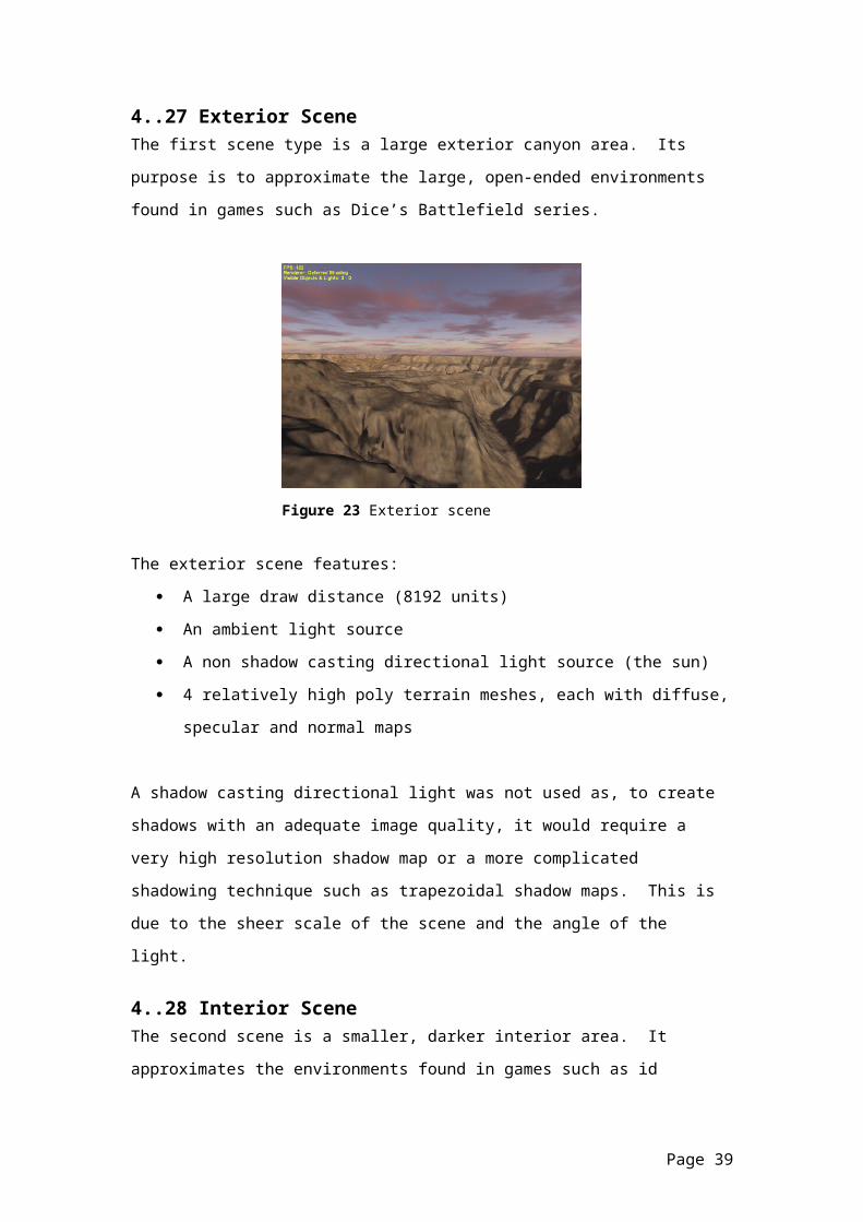
4.3.27 Exterior SceneThe first scene type is a large exterior canyon area. Its purpose is to approximate the large, open-ended environments found in games such as Dice’s Battlefield series.

Page 30

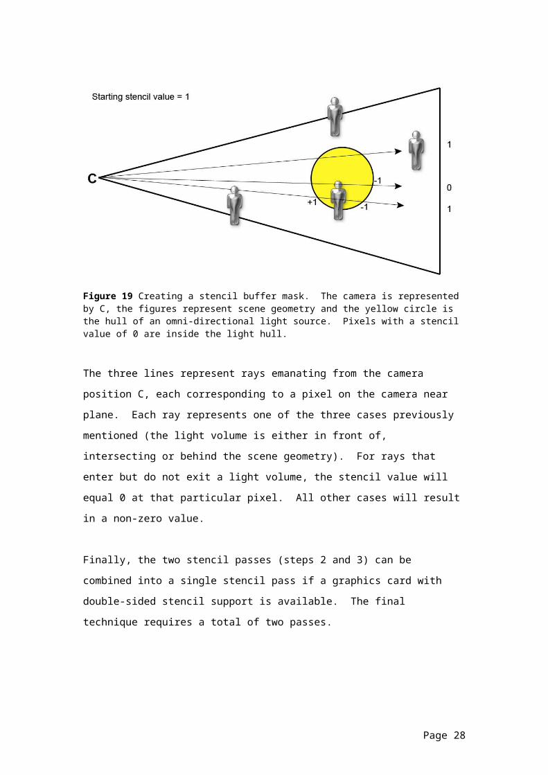
Figure 23 Exterior scene

The exterior scene features: A large draw distance (8192 units) An ambient light source A non shadow casting directional light source (the sun) 4 relatively high poly terrain meshes, each with diffuse, specular

and normal maps

A shadow casting directional light was not used as, to create shadows with an adequate image quality, it would require a very high resolution shadow map or a more complicated shadowing technique such as trapezoidal shadow maps. This is due to the sheer scale of the scene and the angle of the light.

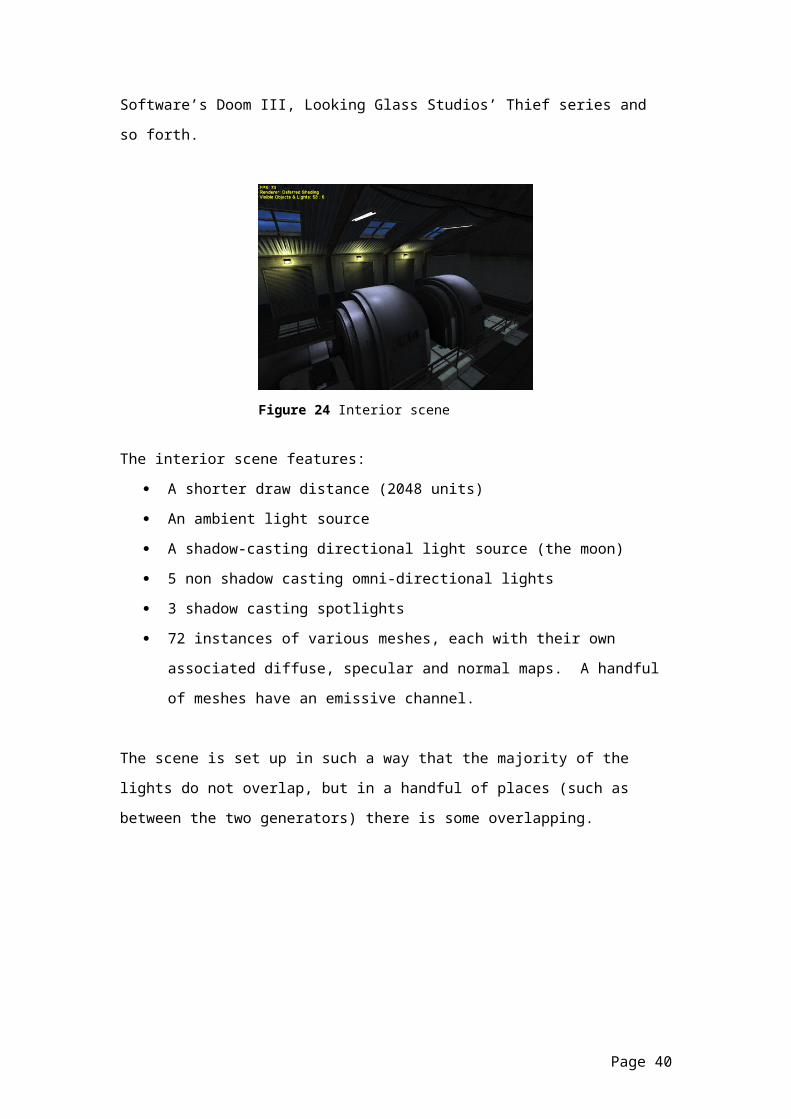
4.3.28 Interior SceneThe second scene is a smaller, darker interior area. It approximates the environments found in games such as id Software’s Doom III, Looking Glass Studios’ Thief series and so forth.

Page 31

Figure 24 Interior scene

The interior scene features: A shorter draw distance (2048 units) An ambient light source A shadow-casting directional light source (the moon) 5 non shadow casting omni-directional lights 3 shadow casting spotlights 72 instances of various meshes, each with their own associated

diffuse, specular and normal maps. A handful of meshes have an emissive channel.

The scene is set up in such a way that the majority of the lights do not overlap, but in a handful of places (such as between the two generators) there is some overlapping.

Page 32

Chapter 5 : Results

5.1 PerformanceThe following results were collected using NVPerfHUD.

5.3.1 Exterior SceneBatching Deferred Shading Forward ShadingDraw Primitive calls

17 16

Resolution Deferred Shading perf. Forward Shading perf.800 x 600 176 fps / 5.7 ms 226 fps / 4.4 ms1024 x 768 103 fps / 9.7 ms 213 fps / 4.7 ms1280 x 960 78 fps / 12.8 ms 176 fps / 5.7 ms1600 x 1200 46 fps / 21.7 ms 128 fps / 7.8 ms

Performance breakdown of deferred shadingResolution Vertex

ShaderPixel Shader Texture Unit Raster Ops

800 x 600 2.3 ms 2.9 ms 1.3 ms 1.2 ms1024 x 768 2.3 ms 4.5 ms 2 ms 1.8 ms1280 x 960 2.3 ms 7.1 ms 3.2 ms 2.7 ms1600 x 1200 2.3 ms 11 ms 5 ms 4.1 ms

Performance breakdown of forward shadingResolution Vertex

ShaderPixel Shader Texture Unit Raster Ops

800 x 600 3 ms 0.9 ms 0.4 ms 0.5 ms1024 x 768 3 ms 1.3 ms 0.7 ms 0.7 ms1280 x 960 3 ms 2 ms 1 ms 1.1 ms1600 x 1200 3 ms 3 ms 1.5 ms 1.7 ms

Page 33

5.3.2 Interior Scene (Shadows Enabled)Batching Deferred Shading Forward ShadingDraw Primitive calls

346 531

Item / Measure Deferred Shading perf. Forward Shading perf.800 x 600 132 fps / 7.6 ms 100 fps / 10 ms1024 x 768 82 fps / 12.2 ms 51 fps / 19.6 ms1280 x 960 53 fps / 18.8 ms 47 fps / 21.3 ms1600 x 1200 31 fps / 32.3 ms 28 fps / 35.7 ms

Performance breakdown of deferred shadingResolution Vertex

ShaderPixel Shader Texture Unit Raster Ops

800 x 600 0.6 ms 6.1 ms 1.7 ms 2 ms1024 x 768 0.6 ms 9.7 ms 2.7 ms 3 ms1280 x 960 0.6 ms 14.7 ms 4.2 ms 4.4 ms1600 x 1200 0.6 ms 21.5 ms 6.5 ms 6.4 ms

Performance breakdown of forward shadingResolution Vertex

ShaderPixel Shader Texture Unit Raster Ops

800 x 600 1.6 ms 7 ms 1.7 ms 2.1 ms1024 x 768 1.6 ms 10.8 ms 2.6 ms 3.2 ms1280 x 960 1.6 ms 16 ms 4 ms 4.8 ms1600 x 1200 1.6 ms 24.3 ms 6 ms 7.1 ms

5.3.3 Interior Scene (Shadows Disabled)

Batching Deferred Shading Forward ShadingDraw Primitive calls

110 302

Page 34

5.4 Number of Lights & Screen Coverage

5.4.1 One spot light The spotlight is framed in the camera so that it is occupying roughly half of the screen. The camera is then moved forward so that it is completely enclosed in the spotlight (requiring the pixel shader to be executed for all pixels).

Configuration Deferred Shading perf.

Forward Shading perf.

Small screen space coverage

123 fps / 8.1 ms 68 fps / 14.7 ms

Large screen space coverage

102 fps / 9.2 ms 156 fps / 6.4 ms

5.4.2 Two spotlights, overlapping (camera pointing at overlap)The two spotlights are viewed from above, looking down. The overlap is centred in the view and initially occupies a small portion of the screen. On zooming in, the overlap increases in size, occupying the entire screen.

Configuration Deferred Shading perf.

Forward Shading perf.

Small screen space coverage

68 fps / 14.7 ms 47 fps / 21.3 ms

Large screen space coverage

60 fps / 16.7 ms 80 fps / 12.5 ms

5.5 Deferred Shading Stencil Lighting Optimisation:To test the stencil optimisation, the camera was placed such that a ‘floating’ spotlight covered the majority of the screen (i.e. the spotlight, while visible, did not actually light any visible pixels).

Page 35

Figure 25 Stencil Light volume (highlighted in orange). Note the light volume is ‘floating’ and thus no pixels will be considered for lighting.

Using a resolution of 1024 x 768, both passes of the stencil optimised light hull were completed in a total time of 0.16 ms, requiring two draw primitive calls in total. Using a non-stencil optimised implementation incurs a performance penalty of roughly 2 ms, but only requires a single draw call.

5.6 Forward Shading Illumination Sets:Using a resolution of 1024 x 768, rendering a single frame of the interior scene without utilising the illumination sets (i.e. using brute force) took a period of 27 ms, falling to 19.6 ms when enabled.

Page 36

5.7 Image FidelityThe following images are cropped screenshots grabbed from the application. The original resolution was 1024 x 768.

The left and right panes of each image show the same scene captured using the deferred and forward shading renderers respectively.

Figure 26 Omni-directional lighting. The images are almost identical.

Figure 27 Spot lighting. The door mesh is sparsely tessellated and, as a result, it is poorly lit by the forward shading renderer.

Figure 28 Directional lighting. The specular lighting is slightly different, but the difference is barely noticeable.

Page 37

Chapter 6 : Analysis

6.1 BatchingFirstly, there is something of a surprise in that the exterior scene requires one fewer draw primitive call (16 versus 17) when using forward shading despite the forward shading renderer requiring two passes per piece of geometry (one for the ambient term and one for the directional light). On examining why this happens, the result becomes clearer. This result occurs due to the single directional light source and relatively small number of meshes – there are only four. Adding further lights to the scene would immediately tip the balance in favour of deferred shading in terms of batching efficiency, even if the lights only affected a couple of meshes.

On examining the results of the interior scene containing various local light sources, the pattern is much more familiar and closely mirrors the assertions of previous studies. With shadowing enabled, the forward shading renderer requires 531 drawprimitive calls compared to the 346 of deferred shading. This represents a significant increase – 53%.

However, this does not tell the full story as many of the draw calls are related to shadow map generation and are thus a common cost. By eliminating the shadow-map generation draw calls, it is plainly evident that the gap is wider still. The forward shading renderer requires 302 draw primitive calls compared to the deferred shading renderer’s 110 – an increase of 274%. If the shadow set generation in the sample application was more robust, the result would probably be somewhere between the two figures. This is due to the fact that the current implementation does not create an accurate shadow set unless the light’s centre is inside the view frustum, thus more objects are added to the shadow list than is necessary.

As stated in the previous section, the sample application is 100% GPU limited meaning the batching efficiency has absolutely no bearing on the framerate in this instance. However, in a real game where various sub-systems of a game engine compete for resources, a large number of batches may result in the game becoming CPU limited (Wloka, 2003). In

Page 38

an example of breaking down the costs of batching, Wloka states that a 2 Ghz CPU utilising 20% of its processing time batching can provide 333 batches per frame at 30 frames per second. While the sample application is not rigorously optimised, the implications are obvious – deferred shading inherently makes far fewer draw calls. As previously asserted by Shishkovtsov (2005), deferred shading does reduce the CPU usage related to submitting batches.

In addition to the measurable performance aspects, the batching was found to be much more straightforward to manage in conjunction with deferred shading. With deferred shading, there is one single pass to fill the g-buffer meaning objects can be sorted by various criteria and the ordering is rarely broken.

Contrast this with forward shading. To form an ordered list, the objects must be broken down into their constituent parts (vertex and index buffers, matrices, textures etc). Separating an object like this loses the original structure (i.e. to which object does this vertex buffer belong?) and so, although the list may be sorted by a specific key (such as diffuse texture), it is difficult to re-use such a sorted list for further rendering. Instead, during further lighting passes, it is probably more convenient just to break the objects apart once more. This requires re-sorting the objects – redundant work.

Furthermore, when rendering further lighting contributions, since the type of object being considered for lighting is often changing, it is more difficult to group primitives by state since each light may be affecting numerous objects whose resources are entirely different to one another. Deferred shading does not have such a problem as the lighting is entirely disconnected from the G-Buffer pass. The only changing resources relate to shadow mapping.

6.3 Rendering PerformanceThe performance results correspond with the predictions made. There is little room for debate pertaining to rendering exterior scenes with few light sources – deferred shading’s performance is weak compared to forward shading.

Page 39

At lower resolutions the performance gap – 5.7ms versus 4.4ms per frame – is rather low due to the cheap G-Buffer pass and the fact that the vertex transformation costs accounts for a sizeable slice of the frame time. However, as the resolution increases, the pixel processing capability of the graphics card soon becomes the overriding performance factor. At 1600 x 1200, the forward shading renderer renders at almost three times to the speed of the deferred shading renderer.

Looking at the performance statistics, it becomes clear that the deferred shading performance decreases almost linearly as the number of pixels in the frame buffer increases. The time spent on texture unit and rasterisation increases in much the same fashion. That is to say, deferred shading is heavily limited by the rate at which graphics cards can perform various operations on pixels. Although the deferred shading renderer does eek out a small advantage in vertex transformation costs, it is dwarfed by the losses elsewhere.

The situation is reversed, though not as dramatically, when numerous non-overlapping lights are present in the interior scene. Deferred shading is significantly faster at lower to medium resolutions but, as the resolution increases beyond 1280 x 960, the results begin to converge.

6.3.1 Performance & Screen Space CoverageIt is very interesting to note just how predictable the performance becomes in terms of the area covered by each light. Whereas, in a dynamic game, forward shading is always at the mercy of too many lights affecting too many objects, deferred shading’s costs are far more predictable. As was hypothesised, framing several lights onscreen yields incurs little in the way of performance penalties. A single light occupying the entire screen results in much the same cost as several smaller lights of similar combined area. Since the positioning of many of a game’s lights is often performed in level design software (i.e. statically placed), deferred shading offers an intuitive way to control the game’s performance.

Page 40

6.3.2 Vertex Transformation CostsThe results suggest that the vertex units are extremely underutilised when rendering the sample scenes. However, it is also clear that while the vertex transformation costs are relatively low, the forward shading renderer incurs a performance penalty due to the greater number of required rendering passes. Extrapolating, it is possible that the deferred renderer can increase the geometric complexity without becoming transform bound.

6.3.3 OptimisationsThe optimisations for both the deferred and forward shading renderers proved to be successes. In particular, the stencil masking algorithm significantly reduced the shading costs when a light hull does not intersect scene geometry. 0.16ms versus 2 ms per non intersecting light hull is an enormous increase (and the saving will only grow as the screen space coverage rises).

6.4 Image FidelityFor the most part, when on a level playing field (no AA), the image fidelity was near indistinguishable between renderers. There were some isolated cases where a sparsely tessellated mesh was badly lit by the forward shading renderer, but overall it was felt that the image quality was very similar. The interior scene in particular looked very good.

However, the exterior scene presented some aliasing problems where the canyon mesh met the horizon (possibly due to the strong contrast). It is trivial to enable AA while using forward shading, but it is definitely not possible in conjunction with deferred shading. As such, the scene type may well dictate whether the loss of AA is an acceptable sacrifice. Darker games such as DoomIII tend to be less prone to suffering noticeable aliasing problems, whereas games with high frequency details and fast gameplay may not be so lucky.

6.5 ExtensibilityThe extensibility of forward shading is already well-known. HDR, fogging etc. are all proven performers. Deferred shading proved to be relatively

Page 41

simple to extend. In addition to implementing a standard HDR technique, the G-Buffer was also successfully used as in input into a post processing fog algorithm. Although the effect in question was rather crude, there is no doubt that, using scene depth as an input, sophisticated effects could be created. The only remaining question mark in terms of extensibility is whether the G-Buffer offers enough parameters to satisfy a wide variety of material types and effects. Although more render targets can be added to the G-Buffer, the extra flexibility comes at the cost of rendering performance.

Page 42

Chapter 7 : Conclusion

7.1 SummaryThe goal of this study was to investigate and characterise the main issues associated with the implementation of deferred shading when compared to forward shading. In performing this work, two renderers were created, one supporting deferred shading and the other supporting multiple pass, multiple light forward shading.

Two different scenes were constructed to approximate the conditions found in real-time computer games.

All of the key areas were investigated. These areas included: Scene management, including how batching is organised. Rendering performance in a variety of common situations. Image fidelity. Ease of use Ease with which modern effects were able to be supported.

7.2 ConclusionsScene management was found to be elegant when using deferred shading, but was less so when using forward shading due to the increasing difficulty in grouping primitives to reduce batching. The result was a significantly higher batch count when forward shading required multiple lighting passes. For CPU-bound games, deferred shading definitely offers an advantage.

Modern effects were easily integrated with deferred shading, though it often required an alteration of the algorithm involved. In many cases the alteration involved performing a calculation per-pixel rather than per vertex.

In terms of rendering performance, deferred shading is definitely not a universal solution. As the resolution increases, the graphics card becomes increasingly limited by its fill rate. In handling outdoor scenes and scenes with relatively few light sources, forward shading is still a far superior

Page 43

performer. The cost of filling the G-Buffer is a large burden so deferred shading should not be considered in these circumstances.

However, when numerous small, non-overlapping lights are required, deferred shading looks a much more attractive prospect; it outperforms forward shading in many circumstances, though at higher resolutions the performance difference begins to disappear. The screen space coverage of the lights also introduces a predictability in terms of shading complexity, meaning developers may be able to minimise the rendering costs through clever light placement and level design, whereas with a forward shading renderer it is often more difficult to constrain the number of objects coming into contact with any given light.

The image quality is almost indistinguishable between the two renderers in most situations, though deferred shading’s incompatibility with AA is definitely a concern. The type of scene, art style and various other factors should be considered before committing to deferred shading as the loss of AA may make the image quality drop significantly. Also, while the geometry used in the sample application was not particularly complex, the reduced work performed by the vertex units when using the deferred renderer would appear to validate the claims that when multi-pass lighting is required, deferred shading can provide a more visually complex scene without a significant performance hit.

7.3 Recommendations for Future WorkWith many of the basic issues (such as performance and extensibility) now better understood, suggestions for future work includes:

Optimising the directional light shader. Shishkovtsov (2005) suggests creating a stencil mask to reduce the number of wasted pixels shaded by directional lights. As previously mentioned, full screen lights are very expensive to calculate and so this could be a very profitable optimisation.

Implementing multiple shading models using Shader Model 3.0’s dynamic branching capability. Although some cursory testing was carried out where a materialID was stored in the G-Buffer and the correct material shader identified, this was not included in the report as not enough work

Page 44

was done to make any judgements. If branching is reasonably coherent, this should be possible to implement and will increase flexibility in representing a larger number of material types.

Atmospheric & volumetric effect rendering. Wenzel (2006) details numerous interesting effects which can be implemented using scene depth stored in a render target.

Page 45

Appendix A : Project Proposal

IntroductionThe graphical advancements of recent years appear to show no sign of halting. However, as shaders become more sophisticated, lighting models more complex and geometry more detailed, the impressive processing power offered by today’s graphics cards may not be enough to maintain the charge towards photo-realism. Shading dominates the cost of rendering a scene. The figures relating to graphics cards reinforce this point; 50% of a modern graphics card’s die area is devoted to texturing/shading. Mark and Moreton (2004, p. 31) estimate that this figure may increase to something in the region of 90% in the future.

In the real world, the colour the human brain perceives at any given point is dependant on numerous factors. When light interacts with a surface, a complicated light-matter dynamic takes place; this process depends on the qualities of both the light and the surface. Light striking a surface is typically absorbed or reflected, though it can also be transmitted. In general, when an observer looks at an illuminated surface, what is viewed is reflected light (Wynn, 2000, p. 2). In real-time computer graphics, shading is defined as an approximation of the colour and intensity of light reflected toward the viewer for each pixel representing a surface (Lengyel, 2004, p. 161).

Forward shading schemes can be considered immediate; the shading produced by each pass is calculated as it is encountered, the intermediate calculations discarded and the results blended with the existing framebuffer contents. That is to say, the shading contribution of an object is calculated in step with the geometric transformations and rendering of that object.

Deferred shading is simply the decoupling of the transformation of an object and the calculation of its shading contribution to the scene, hence the name deferred shading. Instead of transforming the object and immediately calculating the shading contribution to the scene, the object’s

Page 46

per-pixel attributes (such as position, diffuse, normal, gloss etc.) are written to an intermediate “fat” buffer (or g-buffer) and stored for further use. The g-buffer is typically comprised of a series of renderable textures. The application is then free to refer to the g-buffer’s contents to calculate the contribution of each light to the scene during a separate lighting pass (Heargreaves & Harris, 2004, p. 12).

The aim of the project is to comparatively evaluate deferred and forward shading with a view to characterising the issues associated with each in the context of real-time computer games. This will be achieved by implementing each technique in sample applications which, in turn, tackle common problems found in real-time games. The performance and visual fidelity of each technique can then be compared for each particular situation. Just as importantly, by creating these applications it will provide an insight into the more conceptual and less readily graspable areas of batch management, ease of use, compatibility with common effects (primarily shadow rendering) and so forth.

Put simply, the aim is to better understand the technical and conceptual strengths and weaknesses of deferred shading when contrasted with prevalent methods of forward shading.

MotivationDeferred shading isn’t a new technique; it was first suggested by Deering et al. (Siggraph 1988) for use in offline rendering. In years gone by, deferred shading has been prohibitively expensive to implement on the PC platform due to graphics cards lacking the required feature set and processing power. With the advent of Geforce 6 class graphics cards, deferred shading has become a realistic proposition for use with PC games. At the present time, only a handful of games such as Red Storm’s “Ghost Recon Advanced Warfighter” have used deferred shading. Many commentators have struggled to reach a consensus regarding deferred shading’s worth or future; as Nvidia’s “6800 leagues” presentation states, “More research is needed!” (Hargreaves & Harris, 2004, p. 36).

Page 47

Indeed, just as deferred shading is becoming feasible, forward shading is beginning to display various shortcomings. To understand why examining deferred shading is of interest to developers, it is necessary to examine the current problems associated with forward shading.

There are two primary methods utilised when shading scenes in currently available real-time games: Single pass, multiple light (SPML) and multiple pass, multiple light (MPML). SPML applies all lighting to the scene in a single shader which avoids the duplication of transforms associated with multiple passes. While this may seem attractive, the SPML shader must be able to handle every single combination of lighting inputs. This typically results in the generation of thousands of shaders to handle all possible combinations. This method is also largely incompatible with modern shadowing techniques and has a tendency to overflow shader length limitations (Heargreaves, 2004, p. 3). The alternative of MPML often requires several rendering passes to cumulatively shade an object; when using traditional MPML forward shading schemes, the results of transforming vertices and calculating normals, parallax and other data cannot be stored for future reference. When an object is illuminated by multiple lights, this intermediate data is common to each pass, but must be recalculated and discarded each and every pass. When triangle meshes are comprised of several thousand vertices and refer to multiple texture maps (many of which require decompression and additional computation each time they are referenced), this extra computation soon becomes noticeable. In a scene with L lights and N objects, the worst case complexity is N * L rendering passes (Hargreaves, 2004, p. 4).

Even worse, overdraw (the action of drawing the same pixel more than once) is almost guaranteed to occur when forward shading is utilised. As shaders become ever more complex, pixels that are repeatedly filled represent a costly waste of resources. In scenes featuring significant overdraw, the fill rate is often a bottleneck (Latta, 2004, p.119),

Page 48

In addition to these technical drawbacks, a modern MPML forward shading renderer also requires significant behind the scenes management. For example, the scene is usually batched per object or by light. One may be better than the other in any given situation, but the choices are mutually exclusive. The process of calculating batches is not a trivial problem to solve, nor is it free in terms of CPU time; each object must be checked against each light to determine whether it is illuminated. When dynamic lights and/or objects are involved this batch creation must be calculated at runtime. Shishkovtsov (2005, p. 144) states that many games are CPU bound and techniques like deferred shading can potentially ease the load.

In the past, this hasn’t been a notable problem as fully dynamic lighting wasn’t feasible. However, ever since Doom III debuted with its fully dynamic, unified lighting model, developers have been working on ever-more sophisticated lighting schemes. As the number of dynamic lights increases, forward shading begins to look a little unwieldy, both in terms of batching and technical constraints.

If game developers wish to maintain good performance with visuals to match, techniques that can potentially ease or eliminate these problems must be considered.

Research QuestionWhen implementing deferred shading as a replacement for forward shading in real time computer games, what is a characterisation of the issues involved?

In answering the question, the research will focus on these issues:

Scene management, including how batching is organised. Rendering performance in a variety of common situations. Image fidelity. Ease of use, and ease with which modern effects such as shadow

mapping were able to be added to the application (i.e. extensibility).

Page 49

The rationale for the selection of these issues for investigation is that they all have a significant impact on the development process or the quality of the finished game. If a technique is relatively simple to implement and extend, it aids developer efficiency. Likewise, the player of the game will expect good image quality and interactive frame-rates.

Project ExecutionTo address the question, it is necessary to evaluate several important issues common to scene rendering in real-time games. This will be achieved through the creation of test applications which emulate common scenarios developers must tackle in their games. These applications will form the basic deliverables. For example, some situations to use for the basis of evaluating each technique include:

Large, bright, open areas lit only by static environment lighting such as the sun in addition to relatively few localised lights. This would approximate the situations found in sprawling, open-ended games such as Farcry and the Battlefield series.

Interior scenes lit by numerous dynamic, localised lights. This would approximate the conditions found in games such as Doom III and the Thief series of games.

Proposed further deliverables include extensions to the application including:

Altering the number and type (spot, directional and omni) of lights as well as controlling whether the lights overlap one another, giving a more varied set of situations.

Introducing an early z-culling algorithm. This is reported to increase the shading efficiency of forward shading renderers when fill-rate bound due to shading requirements (Sander et al, 2005, p. 1) and is thus important if attempting to compare the two shading methods.

Page 50

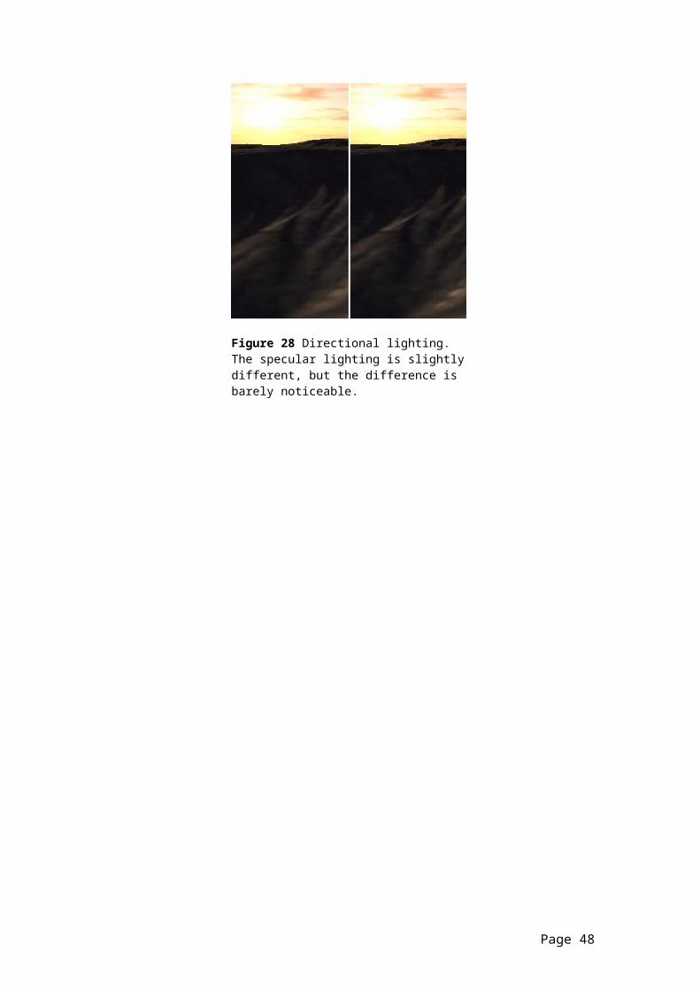
Adding a multiple material branching system for the deferred shading renderer to allow varied material types.

The addition of further common effects such as High Dynamic Range (HDR) lighting with blooming, fogging and particle systems.

The extended deliverables are intended to further test the extensibility and performance of each shading method.

In addition to providing test results, the process of creating these applications will provide useful insights into issues such as ease of use, scene management and other topics that cannot be fully evaluated without firsthand experience.

Evaluation will be performed in several stages. The first is simply to do with performance. By performing tests encompassing a number of common situations and comparing the results to forward shading, it should be possible to better characterise deferred shading’s strengths and weaknesses and make recommendations as to its suitability for various scenarios found in real-time computer games. I.e. it will be possible to determine whether deferred or forward shading is better suited to any given situation.

The assessment of visual aspects is slightly more subjective; images created by each technique will be scrutinised for known artefacts such as aliasing, loss of detail and noticeable inaccuracies.

In addition to the visual aspect, there is the equally important issue of ease of use and the way in which each shading model can be integrated with the application. The main consideration is whether deferred shading complicates or simplifies a number of commonly utilised techniques such as scene management, shadow rendering, effect rendering and so forth. This question will be answered through doing the work and noting the issues as the work progresses.

Issues

Page 51

There are few potential issues that may be encountered during the project’s execution.

Firstly, the scene management system associated with the forward shading renderer is likely to be time-consuming to implement. Significant research must be undertaken to fully understand the batching methods in addition to how to implement them; this research is underway, but the full scale of the task will not be apparent until practical work is started. The study of scene management could be a full project in itself, so achieving the minimum required functionality is the main target (being able to batch fairly efficiently and reducing the amount of objects being considered for shading by each light). Thus far, finding good resources to aid in the implementation of the scene management has proved difficult.

Failure to implement full scene management wouldn’t be a catastrophe in terms of the extensibility or ease of use studies (it would implicitly demonstrate the complexity of implementing such a system), but it would make the comparative performance evaluation somewhat more difficult to conduct. In the event of encountering difficulties in creating the scene management portion, alternatives could be explored such as limiting the number of lights and objects or manually choosing which light influences the shading of each object. If properly done, this would give a reasonable result in terms of the number of rendering passes required. Though this would not approximate the CPU load found in scene management, it would allow the forward and deferred shading costs to be measured in terms of GPU time.

Another possible concern is determining how best to quantify and profile the conceptual aspects, such as ease of use. Whether or not this will prove to be an actual problem will only be apparent once the practical aspects of the project are underway.

Finally, the implementation of shadow maps, HDR and particle systems could be difficult. However, with the exception of deferred particle systems, most of these techniques are very well-documented. It is simply a matter of good planning and time management. With the exception of

Page 52

shadow maps, failure to implement these effects will not cripple the project as they represent additional, rather than basic deliverables.

Resource RequirementsNo specialist resources are required. A personal computer with a Geforce 6 card (or better) will adequately handle any test applications featuring dynamic branching and multiple render targets.

Page 53

Appendix B : Selecting a G-Buffer Format

Choosing the format and number of render targets was one of the major decisions that had to be made when implementing the deferred shading renderer as it pervades the rest of the implementation. This is due to the fact that data must be read from the G-Buffer every time the scene attributes are required.

It is possible to store the data in a variety of configurations and co-ordinate spaces; each has its own advantages and disadvantages. Using render targets with a larger bit depth can improve the quality of the results, but may introduce bandwidth penalties or suffer from manipulation problems due to current hardware limitations (e.g. blending 128 bit render targets is currently unsupported). Likewise, it is possible to trade storage for some extra computation via packing. A thorough examination of G-Buffer formats could fill a chapter in itself, but it is not the focus of this project. Hargreaves & Harris (2004) and Shishkovtsov (2005) both recommend the use of 64-bit floating point A16R16G16B16F textures on modern GPUs.

It is obviously overkill to store diffuse textures (which themselves are often compressed to one of the DXT formats, using 4 to 8 bits per pixel) and normals at 64 bits per pixel, but at the present time, there are certain limitations to be taken into account when choosing the format of multiple render targets (MRTs). While it is possible to choose a separate format for each render target, the bit depths of all MRTs must be the same. Thus, if using a series of 32 bit render targets, it is perfectly legitimate to store the diffuse colour using a A8R8G8B8 format alongside a R32F texture for depth, as the respective channels of each format sum up to 32 bits per pixel. Though the size and number of the channels differ, the combined bit depth is the same.

For the artefact, as the position render target is 64 bits per pixel, this restricts the format of the other render targets that make up the G-Buffer.

Page 54

Since there is no currently available format of a similar bit depth that’d be more suitable, all G-Buffer render targets use the same format.

Page 55

Appendix C : Creating Light Volumes

Light volumes are 3D representations of any given light’s area of influence. They are required for use in the process of optimising lighting shaders for the deferred renderer.

Omni-directional Lights : SpheresTo represent a sphere, a mesh is created using the D3DXCreateSphere() function. Since all spheres are alike, it is simple to scale & translate the sphere to represent an omni-directional light of arbitrary position and radius.

// On application start, create sphere mesh with radius of 1.0f

D3DXCreateSphere( m_pDevice, 1.0f, 16, 8, &m_pSphereMesh, NULL );

// When the sphere is to be rendered:

// Scale up the mesh very slightly to avoid borders due to insufficient tesselation

float fScale = pLight->m_fMaxRange * 1.1f;

// scale light volume mesh to match light's max rangeD3DXMATRIX scale, translate, sphereMatWVP;

D3DXMatrixTranslation( &translate, lightWorldPos.x, lightWorldPos.y, lightWorldPos.z );D3DXMatrixScaling( &scale, fScale, fScale, fScale );sphereMatWVP = scale * translate * matView * matProjPersp;

V( pDeferred->SetMatrix( hWVP, &sphereMatWVP ));

Spotlights : ConesA spotlight hull can be defined using two parameters, the spotlight’s maximum range and its outer angle. If a spotlight has a maximum range of D and its tip is located at the origin with the cone extending in the positive Z direction, then its remaining vertices can be shown to lie in the XY plane at a distance of +D from the origin. Since the maximum range and the angle of the cone is already known, the radius R of the base can be determined by using basic trigonometry. The vertices making up an approximation of a circle are then traced out in the XY plane using the parametric equation of a circle. The indices are calculated for both the cone and the cap and encapsulated in an ID3DXMesh object.

Page 56

// On application start, create the cone mesh on a per light basis

ID3DXMesh* CScene::CreateConeMesh(float fOuterAngle, float fMaxRange){

HRESULT hr = S_OK;

// check that the data is validif( fMaxRange < 0.1f || fOuterAngle < 0.01 ){

return NULL; }

// Form the cone out of a triangle fan, specifying the tip of the cone first, then winding our way around the circle

float fRadius = tan( fOuterAngle * 0.5f ) * fMaxRange;

vector< D3DXVECTOR3 > coneVerts;coneVerts.clear();

// the circle will be traced out on the XY plane at a distance of fMaxRange from the origin so each point will be ( X, Y, fMaxRange )

float fTwoPi = D3DX_PI * 2.0f;float fIncrement = fTwoPi / kiConeFaces;float fParameter = 0.0f;

// the tip is always (0,0,0) so fill it out manuallyconeVerts.push_back( D3DXVECTOR3( 0.0f, 0.0f, 0.0f ));

// then fill out the 2nd to the last verticesfor( UINT i = 1; i < kiConeVertices; i++ ){

D3DXVECTOR3 newPoint;

newPoint.x = fRadius * cos( fParameter );newPoint.y = fRadius * sin( fParameter );newPoint.z = fMaxRange;

coneVerts.push_back( newPoint );

// clockwise winding orderfParameter -= fIncrement;

}

ID3DXMesh* pMesh = NULL;

// We've now got the vertices to place in the mesh.// Create the MeshV( D3DXCreateMesh( kiConeTotalFaces, kiConeFaces * 3, D3DXMESH_WRITEONLY , vePos, m_pDevice, &pMesh ));

posVertex* vert;V( pMesh->LockVertexBuffer( 0, (void**)&vert ));

// copy all unique vertices to the vertex bufferfor( UINT i = 0; i < kiConeVertices; i++ ){

// first vert in trivert[i] = coneVerts[ i ];

}

V( pMesh->UnlockVertexBuffer( ) );

Page 57

vector< UINT > coneIndices;coneIndices.clear();

// fill out the indices per facefor( UINT i = 0; i < kiConeFaces - 1; i++ ){

coneIndices.push_back( 0 );coneIndices.push_back( i + 1 );coneIndices.push_back( i + 2 );

}

// fill out the last face manuallyconeIndices.push_back( 0 );coneIndices.push_back( kiConeFaces );coneIndices.push_back( 1 );

// now fill out the indices for the cap facesfor( UINT i = 0; i < kiConeCapFaces; i++ ){

// The cone cap is aligned with our view vector (+z), so reverse the order of the vertices to generate the correct winding

coneIndices.push_back( i + 3 );coneIndices.push_back( i + 2 );coneIndices.push_back( 1 );

}

WORD* indices = 0; V( pMesh->LockIndexBuffer( 0, (void**)&indices ));

for( UINT i = 0; i < coneIndices.size(); i++ ){

indices[i] = coneIndices[i];}

V( pMesh->UnlockIndexBuffer( ));

return pMesh;}

// When rendering a spot light, rotate & position the cone mesh in the world

// to correspond to the light’s position & orientation, then render it

D3DXMATRIX rotate, translate, matWVP;

D3DXMatrixRotationYawPitchRoll( &rotate, pLight->m_fYaw, pLight->m_fPitch, 0.0f );D3DXMatrixTranslation( &translate, lightWorldPos.x, lightWorldPos.y, lightWorldPos.z );

matWVP = rotate * translate * matView * matProjPersp;V( pDeferred->SetMatrix( hWVP, &matWVP ));

Page 58

Appendix D : The Phong Lighting ModelPhong lighting is an empirical local illumination model which is used extensively in computer graphics and, in particular interactive computer games.

The basic Phong lighting equation gives the intensity of light reflected by any given point on a surface as the sum of the ambient, diffuse and specular terms.

Figure 29 (Nuydens, n.d) : The phong shading model.

The Phong lighting model requires four inputs to calculate the lighting value for a surface:

N = Surface normal vectorL = Negated light vectorV = Negated view vectorR = Light reflection vector

The intensity, I, is calculated using the basic equation:

Page 59

I = A + D + S.

Ambient, AThe ambient term is used to approximate the effect of indirect light reflections. It is represented using a constant colour value that is applied to the entire scene.

A = Ambient light * Ambient material.

Diffuse, DThe diffuse term approximates the reflectance of light equally in all directions (i.e. the value is independent of the view direction). The diffuse value is based on the angle between the surface normal and the negated light direction. Performing a dot product between these two vectors gives a term by which the diffuse light colour and diffuse material is modulated.

D = Diffuse light * Diffuse material * max(N.L, 0)

Specular, SThe specular term is used to represent the ‘shininess’ of a surface. Although this method is empirical in its nature, the effect is satisfactory. Put simply, the specular term approximates how much light reflects off the surface and reaches the viewer’s eye – it is view dependent. As the reflection and view vectors converge, the surface’s specular term grows and, as a result, the surface appears glossy. Finally, the power function is used to create a distinct falloff curve. This is named the specular exponent. Larger values of n create smaller, sharper highlights.

S = Specular light * Specular material * max((R.V), 0)n

Specular / Gloss MappingWhile certain surfaces appear to possess a uniform glossiness (for example, a polished floor or an immaculate cue ball on a snooker table), many surfaces do not. A metallic wall featuring rusted areas will have varying degrees of glossiness depending on the smoothness of the metal, the state of the paintwork and degree of rust etc. A method to represent

Page 60

the glossiness of a surface on a per-pixel basis is specular mapping (a.k.a. gloss mapping). A specular map is simply a texture map whose per-pixel contents allow the modulation of the specular term. If g = the gloss value (ranging from 0 to 1), then the modulated specular term is g*S. A pixel with a gloss value of 0 has no specular lighting, whereas a pixel with gloss value 1 has full specular lighting.

This gives:I = A + (D + g*S)

AttenuationUnlike global light sources (such as ambient and directional lighting), local lighting requires distance attenuation. There are various approximations used in computer graphics. For a surface located a distance of d units from the light source, some common attenuation functions include:

1. 1 / (a2d + bd + c), 2. 1 / d2

3. max( 0, 1 – (d / maxRange))

Where a, b and c are the quadratic, linear and constant user-specific lighting coefficients and maxRange is the maximum distance the light’s rays can travel.

The attenuation calculation will yield a term in the range 0 to 1. The diffuse and specular terms are modulated by the attenuation, giving:

I = A + attenuation * (D + S)

SpotlightsIn addition to the previously mentioned parts of the equation, spotlights require an additional spotlight attenuation term. Spotlights emit light in a cone shaped area. When evaluating a point on a surface, the closer the point to the centre of the spotlight, the greater the intensity.

Page 61

Figure 30 (Nuydens, n.d) : The spotlight cone. A is the unit direction vector, c represents the cone angle.

As the point tends towards the cutoff point c, which is equal to the spotlight’s outer cone angle, the intensity tends towards 0. A spotlight falloff factor, f, is also used to determine the way in which the light attenuates towards the edge of the cone (much in the same way as the regular attenuation function determines the way the intensity changes as a function of distance). If the position is outside the outer cone cut-off point, the intensity is 0. If a point is somewhere between the inner and outer cone angles, the power function is used to calculate the intensity.

The result gives:

1. If( -L.A ) > cos (c)a. spot = (-L.A)f

2. elsea. spot = 0

A smoothing function such as HLSL’s smoothstep intrinsic or a gradient texture can also be used to retrieve the intensity for any given value.

The final spotlight lighting equation is:I = A + attenuation * spot * (D + g*S)

Page 62

Appendix E : NVIDIA NVPerfHUDNVPerfHUD is a performance & analysis tool provided by the NVIDIA graphics card manufacturer. It is compatible with Geforce5+ series cards, though to access the full feature set, a Geforce6+ card with an NVPerfHUD enabled driver is required

The application is free and can be downloaded from the following location: http://developer.nvidia.com/object/nvperfhud_home.html

Basic performance graphs can be accessed by viewing the default screen or by pressing F5. These performance graphs display the number of draw primitive calls per frame and a batching histogram is also available.

In addition to providing basic performance statistic, in conjunction with a Geforce6 series card and a special driver, NVPerfHUD offers various ways to analyse the cost of a frame. By accessing the frame profiler (F8) it is possible to view the total time per frame and the time spent at every stage of the pipeline right down to time spent per primitive.

By using the frame profiler, it is relatively easy to determine the bottleneck that is slowing down the frame. It is also simple to determine how well an optimisation (such as stencil masks for light hulls) is performing.

Appendix F : PC Specification

Specification of the development PC used to collect the results:

Description Development PC SpecificationProcessor AMD Opteron 165 (dual core) @ 2.55

GhzMotherboard MSI Neo2 Platinum (Socket 939)Graphics card NVIDIA 6800 Ultra (Forceware version

93.50)RAM 2 x 1 GB PC 3200Operating System

Windows XP (Service Pack 2)

Page 63

Appendix G : The Shading DemoRun the application by double clicking on the “Win32.exe” file. Also, if NVPerfHUD is available, the application may be started with the NVPerfHUD driver by dragging the win32.exe icon over the NVPerfHUD icon. It should be noted that switching renderers results in the deferred renderer’s performance suffering. This is due to the way in which the resources are created. If benchmarking is required, it is recommended that the user quit the application and restart it to properly re-initialise the deferred renderer.

Controls (can be accessed using the help-controls menu):

Action Key / ButtonMove camera position W A S D‘Run’ Hold left shift while moving

cameraRotate camera Move mouse & hold mouse 2Change renderer RToggle directional lights IToggle omni-directional lights OToggle spot lights PToggle bounding sphere visualisation BToggle light hull visualisation LToggle debug shadow map display ReturnDisplay render targets (Deferred Shading only)

Numpad 0, 1, 2 to display MRTs 0, 1 and 2 respectively.

Display final image (Deferred Shading only)

Numpad 3

The following command line arguments are available, with the options following in brackets:

Set the default renderer:-renderer [deferred | forward | dummy]

e.g. To load the Deferred Renderer: -renderer deferred

Load scene file from scenes folder (do not include path):-scene [filename]

e.g. To load the scenes/canyon.txt scene: -scene canyon.txt

Page 64

Glossary

Term DescriptionAdditive Blending Adding a colour (typically the result of a pixel shader) to

an existing value to combine the two results. Bounding Volume / Primitive

An approximation of an object’s physical form used to perform relatively simple intersection tests. E.g. spheres, boxes and cones.

Flag A variable that indicates membership of a particular group, function or set. Flags are usually Boolean values or unsigned integers, with the individual bit states corresponding to a particular set (a Boolean represents membership of one set, an unsigned integer can represent membership for a maximum of 32 sets [one set per bit]).

G-Buffer A series of render targets storing per-pixel scene attributes such as positions, normals, diffuse colour, gloss, emissive etc.

Light Accumulation Buffer

A render target used to store the results of various lighting calculations. Once finalised, it can be displayed to the user without modification or used as an input into post-processing effects such as fog, HDR etc.

Light Hull / Volume A 3D mesh representation of a light’s area of influence. Light Projection Space

If a light has a view matrix V and a projection matrix P, then a position vector in world space is transformed into light projection space when multiplied by the concatenated VP matrix. If the light is imagined to be a camera, the effect is analogous to vert * world * camera view * camera projection (the standard transformation for clip space).

Light Set The set of objects that are affected by a lightMesh The physical (visible) part of an object. A mesh can be

composed of multiple sub-meshes, each of which is a primitive such as a triangle list.

Normal Mapping Replacing a mesh’s normal vectors with per-pixel normal vectors stored in a texture map.

Object A collection of related items such as meshes, textures, position and orientation in the world etc. used to represent entities (such as avatars, architecture, vehicles

Page 65

etc.) in the scene.Packing Exploiting the structure of a data type/format to store

multiple values rather than a single value. E.g. storing a 3D vector as two floats plus a signed bit which can be used to reconstruct the original 3D vector. This often sacrifices accuracy for size or computation for storage.

Phong Lighting An empirical lighting model extensively used in computer graphics, including real-time computer games.

Pixel Picture element. A pixel is a single element of an image or buffer (usually a colour value, though often interpreted as something different). It should be noted that pixels, texels and fragments are not the same thing, but in this document they are largely used interchangeably as making the distinction was not felt to aid clarity (save for the mapping texels to pixels note).

Rasterise The process of turning triangles into fragments (pre-pixels)

Render The complete process of sending a primitive and other associated inputs (textures etc.) through the entire graphics pipeline.

Scene A collection of objects, lights and various other attributes required to define a scene in the application.

Shadow Map A texture or depth stencil surface containing scene depth values as viewed from a light’s perspective (stored in light projection space).

Shadow Mapping The process of transforming a position vector into light projection space to determine whether it is visible to the light, or occluded.

Shadow Set The set of shadow casting objects for any given light. Stencil Buffer The stencil buffer is the same size as the frame buffer.

The stencil buffer pixel values can be manipulated to form masks, allowing the application to selectively fill and skip pixels.

Tangent Space A co-ordinate space formed by a 3x3 matrix whose basis vectors are the tangent, bitangent and normal of a vertex.

Texel Texture element. A single element of a texture.View Frustum A convex hull formed by the six planes of the camera.

Typically has the shape of a truncated rectangular

Page 66

pyramid.Visible Set The set of visible objects. Visible simply means it passes

the view frustum intersection test and will be visible to the camera.

Page 67

References

Abrash, M (1996) Quake’s lighting model : Surface caching : Bluesnews [online]. Available from: http://www.bluesnews.com/abrash/chap68.shtml [Accessed 28th January 2007]

Arvo, J (1990) A simple method for box-sphere intersection testing, in A. Glassner (eds), Graphics Gems. Boston, Academic Press. p. 335-339

Deering, M et al (1988) The Triangle Processor and Normal Vector Shader: A VLSI System for High Performance Graphics. Proceedings of the 15th annual conference on computer graphics and interactive techniques (SIGGRAPH 88). Vol. 22, Issue 4. New York. The ACM Press. p. 21-30.

Geldreich & Pritchard (2004) Deferred Lighting and Shading : GDC [online]. Available from: http://www.gdconf.com/conference/archives/2004/pritchard_matt.ppt [Accessed 3rd January 2007]

Hargreaves, S (2004) Deferred Shading : GDC [online]. Available from: http://www.talula.demon.co.uk/DeferredShading.pdf [Accessed 3rd October 2006]

Hargreaves, S & Harris, M (2004) 6800 leagues under the sea / Deferred Shading : Nvidia [online]. Available from: http://download.nvidia.com/developer/presentations/2004/6800_Leagues/6800_Leagues_Deferred_Shading.pdf [Accessed 27th September 2006]

“Hellraizer” (2007). RE: Deferred Shading light volumes & optimisations. From: gamedev.net [discussion forums], 13 February 2007. Available from: http://www.gamedev.net/community/forums/viewreply.asp?ID=2890691

Lengyel, E. (2003) Mathematics for 3D Game Programming and Computer Graphics, 2nd edition. Hingham, Charles River Media

Lutz, L (2004) Massively parallel particle systems on the GPU: W. Engel et al (eds): ShaderX3 : Advanced Rendering with DirectX and OpenGL. Hingham, Charles River Media. p. 119-133

Page 68

Mark, W & Moreton, H. (2004) Real-Time 3D Graphics Architecture : [online]. Available from: www.csl.csres.utexas.edu/users/billmark/talks/Graphics_Arch_Tutorial_Micro2004_BillMarkParts.pdf [Accessed 1st December 2006].

Microsoft (n.d.) Directly Mapping Texels to Pixels (Direct3D 9) : Microsoft [online]. Available from: http://msdn2.microsoft.com/en-us/library/bb219690.aspx [Accessed 11th January 2007]

Nuydens, T (n.d) Phong for Dummies : delphi3d [online]. Available from: http://www.delphi3d.net/articles/viewarticle.php?article=phong.htm [Accessed 21st February 2007]

O’Rorke, J (2004) Managing visibility for per-pixel lighting. R. Fernando (editor), GPU Gems Boston, Addison-Wesley. p. 251-255

Phong, B (1975) Illumination for computer generated pictures. Communications of the ACM, 18(6), p. 311-317

Policarpo, F & Fonseca, F (2005) Deferred Shading Tutorial : Fabio Policarpo’s Web Space [online]. Available from http://fabio.policarpo.nom.br/docs/Deferred_Shading_Tutorial_SBGAMES2005.pdf[Accessed 6th October 2006]

Sander et al (2005) Computation Culling with Explicit Early-z and Dynamic Flow Control : ATI Research [online]. Available from http://ati.amd.com/developer/SIGGRAPH05/ATINotes.pdf [Accessed 23rd November 2006]

Shishkovtsov, O. (2005) ‘Deferred Shading in S.T.A.L.K.E.R.’ in: M. Pharr & R. Fernando (eds) GPU Gems 2. London, Addison-Wesley Professional. p. 143-167

Thibieroz, N (2003) Deferred shading with multiple render targets: W. Engel et al (eds): ShaderX2 : Shader Programming Tips & Tricks with DirectX9. Texas, Wordware publishing. p. 251-269.

Thibieroz, N (2007) Clever Shader Tricks : ATI Research [online]. Available from:http://ati.amd.com/developer/brighton/04%20Clever%20Shader%20Tricks.pdf [Accessed 11th February 2007]

Page 69

Wenzel, C (2006) Real-time atmospheric effects in games : AMD [online]. Available from : http://developer.amd.com/assets/D3DTutorial_Crytek.pdf [Accessed 2nd April 2007]

Wloka, M (2003) “Batch, Batch, Batch:” What does it really mean? : NVIDIA [online]. Available from:

http://developer.nvidia.com/docs/IO/8230/BatchBatchBatch.ppt [Accessed 9th December 2006]

Wynn, C. (2000) An Introduction to BRDF-Based Lighting : Nvidia [online]. Available from: http://developer.nvidia.com/attach/6568 [Accessed 27th November 2006]

Zerbst, S. (2004) 3D Game engine programming. Boston, Course Technology Crisp. p. 286.

Page 70

Bibliography

Botsch, M et al (2005) High quality surface splatting on today’s GPUs : Computer Graphics Group [online]. Available from: http://graphics.ucsd.edu/~matthias/Papers/HighQualitySplattingOnGPUs.pdf [Accessed 16th October 2006]

Calver, D (2003) Photo-realistic deferred lighting : Delphi3d [online]. Available from http://www.delphi3d.net/articles/viewarticle.php?article=deferred.htm [Accessed 16th October 2006]

Calver, D (2004) Deferred Lighting on PS 3.0 with High Dynamic Range in: W. Engel et al (eds): ShaderX3 : Advanced Rendering with DirectX and OpenGL. Hingham, Charles River Media. p. 97-105

Francis, N (2006) Deferred Particle Shading : The ignorant game designer [online]. Available from http://unity3d.com/blogs/nf/files/page0_blog_entry73_1.pdf [Accessed 1st December 2006]

Hart, J (2002) Analysis of shading pipelines : [online]. Available from: http://reality.sgiweb.org/olano/s2002c36/ch11.pdf [Accessed 10th November 2006]

Heidreich, W (1999) High-quality shading and lighting for hardware accelerated rendering : Universitat Erlangen-Nurnberg [online]. Available from http://www.cs.ubc.ca/~heidrich/Papers/phd.pdf [Accessed 18th October 2006]

Lengyel, E (2002) The Mechanics of Robust Stencil Shadows : Gamasutra [online]. Available from: http://www.gamasutra.com/features/20021011/lengyel_01.htm [Accessed 13th March 2007]

Sawitus, M (2005) Deferred Shading Demo : M. Sawitus’s website [online]. Available from: http://msawitus.awardspace.com/homepage/deferred_shading_demo.php [Accessed 15th December 2006]

Page 71