Embed Size (px)
Citation preview

On the wave turbulence theory for stratified flows in the ocean
Irene M. Gamba∗ Leslie M. Smith† Minh-Binh Tran‡
January 18, 2019
Abstract
After the pioneering work of Garrett and Munk, the statistics of oceanic internalgravity waves has become a central subject of research in oceanography. The timeevolution of the spectral energy of internal waves in the ocean can be described by anear-resonance wave turbulence equation, of quantum Boltzmann type. In this work,we provide the first rigorous mathematical study for the equation by showing the globalexistence and uniqueness of strong solutions.
Keywords: wave (weak) turbulence theory, quantum Boltzmann equation, wave-waveinteractions, stratified fluids, oceanography, near-resonance
MSC: 35B05, 35B60, 82C40
1 Introduction
The study of wave turbulence has obtained spectacular success in the understanding ofspectral energy transfer processes in plasmas, oceans, and planetary atmospheres. Wave-wave interactions in continuously stratified fluids have been a fascinating subject of intensiveresearch in the last few decades. In particular, the observation of a nearly universal internal-wave energy spectrum in the ocean, first described by Garrett and Munk (cf. [22, 23, 11]),plays a very important role in understanding such wave-wave interactions. The existence ofa universal spectrum is generally perceived to be the result of nonlinear interactions of waveswith different wavenumbers. As the nonlinearity of the underlying primitive equations isquadratic, waves interact in triads (cf. [63]). Furthermore, since the linear internal wavedispersion relation can satisfy a three-wave resonance condition, resonant triads are expectedto dominate the dynamics for weak nonlinearity (cf. [44]).
1Department of Mathematics and Institute for Computational Engineering and Sciences, The Universityof Texas at Austin, TX 78712, USA.Email: [email protected]
2Department of Mathematics and Department of Engineering Physics, University of Wisconsin-Madison,Madison, WI 53706, USA.Email: [email protected]
3Department of Mathematics, Southern Methodist University, Dallas, Texas, TX 75275, USA.Email: [email protected]
1

Resonant wave interactions can be characterized by Zakharov kinetic equations (cf.[71, 46, 42, 10, 69, 68]). The equations describe, under the assumption of weak nonlinearity,the spectral energy transfer on the resonant manifold, which is a set of wave vectors k, k1,k2 satisfying
k = k1 + k2, ωk = ωk1 + ωk2 , (1.1)
where the frequency ω is given by the dispersion relation between the wave frequency ωand the wavenumber k. However, it is known that exact resonances defined by ωk =ωk1 + ωk2 do not capture some important physical effects, such as energy transfer to non-propagating wave modes with zero frequency, corresponding to generation of anisotropiccoherent structures [4, 5, 7, 15, 16, 25, 33, 34, 35, 41, 51, 64, 65], see also [18, 45] foranalytical arguments on reduced isotropic models. Some authors have included more physicsby allowing near-resonant interactions (cf. [13, 32, 40, 36, 37, 38, 39, 47, 57, 53, 54]), definedas
k = k1 + k2, |ωk − ωk1 − ωk2 | < θ(f, k), (1.2)
where θ accounts for broadening of the resonant surfaces and depends on the wave densityf and the wave number k. When near resonances are included in the dynamics, numericalstudies have demonstrated the formation of the anisotropic, non-propagating wave modesin dispersive wave systems relevant to geophysical flows (cf. [12, 27, 32, 55, 56, 57, 58, 59]).
We consider in this paper the following near-resonance turbulence kinetic equation forinternal wave interactions in the open ocean (cf. [13, 36, 37, 38, 40]),
∂tf(t, k) + µkf(t, k) = Q[f ](t, k), f(0, k) = f0(k), (1.3)
in which f(t, k) is the nonnegative wave density at wavenumber k ∈ Rd, d ≥ 2. As proposedby Zakharov in [69] water wave models must include the term µkf = 2ν|k|2f for viscousdamping effects, with ν the viscosity coefficient.
This model equation consist in a kinetic three-wave interaction modelled by an interac-tion (or collision) operator given by the non-local form
Q[f ](k) =
∫∫R2d
[Rk,k1,k2 [f ]−Rk1,k,k2 [f ]−Rk2,k,k1 [f ]
]dk1dk2 (1.4)
with
Rk,k1,k2 [f ] := |Vk,k1,k2 |2δ(k − k1 − k2)Lf (ωk − ωk1 − ωk2)(f1f2 − ff1 − ff2), (1.5)
with the short-hand notation f = f(t, k) and fj = f(t, kj). The singular measure given bythe Dirac delta function δ(·) ensures that interactions are between triads with
k = k1 + k2. (1.6)
The transition probability factor or collision kernel Vk,k1,k2 under consideration is of theform (cf. [38, 13, 37, 40, 36])
Vk,k1,k2 = C (|k||k1||k2|)12 , (1.7)
2

with C is some physical constant.Next, we consider the dispersion law
ωk =
√F 2 +
g2
ρ20N
2
|k|2m2
, (1.8)
where F is the Coriolis parameter, N is the (Brunt-Vaisala) buoyancy frequency, In addition,the parameter m is the reference vertical wave number determined from observations, g isthe gravitational constant, ρ0 is the reference value for density, or equivalently
ωk =√λ1 + λ2|k|2, for λ1 = F 2 , and λ2 =
1
m2
(g
ρ0N
)2
=1
k2z
. (1.9)
where kz cartesian vertical wave number and m = kzg(ρ0N)−1. In the absence of theCoriolis force, i.e. F = 0, the dispersion relation becomes
ωk =|k|m≈ |k|kz
. (1.10)
The operator Lf is defined as
Lf (ζ) =Γk,k1,k2
ζ2 + Γ2k,k1,k2
, (1.11)
with the condition thatlim
Γk,k1,k2→0Lf (ζ) = πδ(ζ).
Thus when Γk,k1,k2 tends to 0, (1.4) becomes the following exact resonance collision operator(cf. [69, 68, 26])
Qe[f ](k) =
∫∫R2d
[Rk,k1,k2 [f ]− Rk1,k,k2 [f ]− Rk2,k,k1 [f ]
]dk1dk2 (1.12)
with
Rk,k1,k2 [f ] := |Vk,k1,k2 |2δ(k − k1 − k2)δ(ωk − ωk1 − ωk2)(f1f2 − ff1 − ff2).
Moreover, the resonance broadening frequency Γk,k1,k2 may be written
Γk,k1,k2 = γk + γk1 + γk2 , (1.13)
where γk is computed in [36] using a one-loop diagram approximation:
γk v c|k|2∫R+
|k|2|f(t, |k|)|d|k|,
3

and c is a physical constant, which can be normalized to be 1. Approximating the integral∫R+
|k|2|f(t, |k|)|d|k| ≈∫R3
f(t, k)dk,
we obtain a formula for γk that will be used throughout the paper
γk = |k|2∫R3
f(t, k)dk. (1.14)
The above formulation of γk indicate the broadening resonance width θ defined in (1.2).Note that the formulation of Γk,k1,k2 is given
Γk,k1,k2 = (|k|2 + |k1|2 + |k2|2)
∫R3
f(t, k)dk, (1.15)
Observe that
√nΓk,k1,k2 ≤ |ωk − ωk1 − ωk2 | ≤
√n+ 1Γk,k1,k2 , n ∈ N,
then1
(n+ 2)Γk,k1,k2≤ Lf (ωk − ωk1 − ωk2) ≤ 1
(n+ 1)Γk,k1,k2,
in other words, function Lf (ωk − ωk1 − ωk2) is mostly concentrated in the interval where
|ωk − ωk1 − ωk2 | ≤ Γk,k1,k2 . (1.16)
In other words, the resonance width θ is proportional to Γk,k1,k2 , which depends on f andk.
This fact will be used in the proof of Propositions 2.3, 2.1 and 3.1.In the field of wave turbulence, the most commonly used asymptotical analysis to derive
the kinetic equation (1.3)- (1.6) is statistical closure of the infinite hierarchy of cumulants,in the weakly nonlinear and long-time limits (see, for example, the review by Newell andRumpf [48]). Evolution of higher-order cumulants can be interpreted as a modification ofthe wave frequency, with real part corresponding to a frequency shift and with imaginarypart corresponding to resonance broadening.A Feynman-Dyson diagrammatic approach may also be used, adapted for turbulence influids by Wyld [66], for more general classical systems by Martin, Siggia and Rose [43], andfor Hamiltonian nonlinear wave fields by Zakharov and Lvov [70]. In the context of acousticturbulence, Lvov, Lvov, Newell and Zakharov [36] considered a one-loop approximation tothe resonance broadening, the form of which is the one to be adopted in our study.
It is noted that wave turbulence equation (1.3) shares a similar structure with thequantum Boltzmann equation describing the evolution of the excitations in thermal cloudBose-Einstein condensate systems (cf. [21, 29, 30, 31, 67, 72]). Our recent progress on theclassical Boltzmann equation (cf. [8, 19, 20, 62]) and the quantum Boltzmann equation (cf.
4

[2, 14, 17, 24, 28, 50, 49, 61, 52, 60]) has shed some light on the open question of buildinga rigorous mathematical study for (1.3). Different from the quantum Boltzmann cases (cf.[61, 2, 14]), which could be considered as the exact resonance case (1.12) with
ωk = ωk1 + ωk2 ,
the energy of solutions for the near-resonance kinetic equation (1.3) is not conserved. Theunderlying shallow-water equations conserve a cubic energy, and the flow restricted to exactresonances conserves the quadratic part of the total energy [65]. However, conservationof the quadratic energy no longer holds when near resonant three-wave interactions areincluded in the dynamics.
We also split Q as the sum of their positive and negative parts, referred to as a gainand a loss operators, respectively:
Q[f ] = Qgain[f ] − Qloss[f ], (1.17)
as is done with the classical Boltzmann operator for binary elastic interactions. Here, thegain operator is also defined by the positive contributions in the total rate of change in timeof the collisional form Q(f)(t, k)
Qgain[f ] =
∫∫Rd×Rd
|Vk,k1,k2 |2δ(k − k1 − k2)Lf (ωk − ωk1 − ωk2)f1f2dk1dk2
+ 2
∫∫Rd×Rd
|Vk1,k,k2 |2δ(k1 − k − k2)Lf (ωk1 − ωk − ωk2)(ff1 + f1f2)dk1dk2.
(1.18)and the loss operator models the negative contributions in the total rate of change in timeof the same collisional form Q(f)(t, k)
Qloss[f ] = fϑ[f ], (1.19)
with ϑ[f ] being the collision frequency or attenuation coefficient, defined by
ϑ[f ](k) = 2
∫∫Rd×Rd
|Vk,k1,k2 |2δ(k − k1 − k2)Lf (ωk − ωk1 − ωk2)f1dk1dk2
+ 2
∫∫Rd×Rd
|Vk1,k,k2 |2δ(k1 − k − k2)Lf (ωk1 − ωk − ωk2)f2dk1dk2.
(1.20)
Inspired by recent work by Alonso and two of the authors of the current manuscript[2] on the quantum Boltzmann equation for cold bosonic gases, whose equation can also bederived by diagrammatic techniques, we present here the existence and uniqueness solutionto a Cauchy problem associated to the model (1.3)-(1.11)
The strategy consists in finding a suitable convex, positive cone, time invariant subspaceST of the Banach space L1
N (Rd), for which the weak turbulence equation has a unique strong
5

solution, where this Banach space has norms defined by the N th moment as the expectationof the N th-power of the dispersion relation, that is for any given density g,
L1N (Rd) := {g ∈ L1(Rd), s.t. ‖g‖L1
N:= MN [g] =
∫RdωNk g(k)dk <∞}, (1.21)
in which we recall the dispersion relation ωk =√λ1 + λ2|k|2 as defined in (1.9). Notice that
when g is positive, both Mn[g] and ‖g‖L1n
are equivalent. Hence, the construction of suchinvariant subspace ST depend on the control of higher order moments defined as follows.
Our solution are global and unique in L1N (Rd) to (1.3), that is the satisfy
∂tf(t, k) = Qgain[f ](t, k) − f(t, k)ϑ[f ](t, k) − 2ν|k|2f, f(0, k) = f0(k) ∈ ST . (1.22)
A fundamental tool to accomplish our goal is to prove that there exists a differentialequation of the following type, for the moments of the solution f of (1.22)
d
dtMN [f ] ≤ C1MN+1[f ]− C2MN+2[f ],
for some positive constants C1, C2, which leads to
d
dtMN [f ] ≤ C3MN [f ],
with C3 being a positive constant. The above inequality then yields an exponential boundon the N -th moment of f
MN [f ] ≤ CeC′T .
In order to do that, estimates on Qgain and Qloss are provided in Propositions 2.3 and 2.1.The proofs of these estimates are based on careful bounds of Lf and Γk,k,k1 , that reduces
to bounding the 0-th moment of f , M0[f ](t), from below by e−(2νR20+4R0)t‖f0χR0‖L1 , where
χR0 is the characteristic function of the ball B(O,R0) centered at the origin with radius R0
so that the quantity ‖f0χR0‖L1 > 0.Finally, on any arbitrary fixed time interval [0, T ], we construct the solution of (1.22)
within a time-dependent invariant set ST , based on the exponential in time upper bound ofMN [f ] and the lower bound of M0[f ].
More specifically, we define first the following two constants, C∗ and C∗, for any givenany R0 by
C∗ :=C0(λ1, λ2)
(1 + e(4νR2
0+8R0)T)
‖f0(k)χR0‖L1
, and C∗ := 4νR20 + 8R0. (1.23)
The specific value of R0 will be determined later to secure the conditions to obtain a timeinvariant region.
6

Hence, for any number R∗ > 0, R∗ > 1, moment order N , and time t > 0, we define theconvex positive cone ST as a subset on L1
N given by
ST :={f ∈ L1
N+3
(Rd)
: S1) f ≥ 0; S2) ‖f‖L1N+3≤ c0(t) := (2R∗ + 1)eC∗t; (1.24)
S3)− ‖f‖L1 ≥ c1(t) :=R∗e−C
∗t
2.}
where the c0(t) is an increasing function and c1(t) is a decreasing function, so St ⊂ St′ for0 ≤ t ≤ t′ ≤ T
Our main result is as follows.
Theorem 1.1 Let N > 0, and let f0(k) ∈ S0∩B∗(O,R∗)\B∗(O,R∗) for some R∗ > R∗ > 0,where B∗(O,R
∗), B∗(O,R∗) is the ball centered at O with radius R∗, R∗ of L1N+3(Rd).
Then the weak turbulence equation (1.3) has a unique strong solution f(t, k) so that
0 ≤ f(t, k) ∈ C(
[0, T );L1N (Rd)
)∩ C1
((0, T );L1
N (Rd)). (1.25)
Moreover, f(t, k) ∈ ST for all t ∈ [0, T ).Since T can be chosen arbitrarily large, the weak turbulence equation (1.3) has a unique
global solution for all time t > 0.
The proof of Theorem 1.1 relies on the following abstract Ordinary Differential Equa-tions theorem in Banach spaces, which provides a framework to developed the existence anduniqueness theory to space homogeneous Boltzmann type equations ranging from the classi-cal Boltzmann equation for binary interaction, to nonlocal kinetic model for rods alignment,to quantum kinetic theory of bosonic cold gases [9, 1, 2, 3].
Applied to the initial value problem (1.3)-(1.16), the framework is given by the followingabstract existence and uniqueness theorem in Banach spaces along the lines proposed by A.Bressan in the unpublished notes [9], whose application to the classical Boltzmann theoryfor hard potential and integrable angular cross section has been recently completed in [3],as follows.
Let E := (E, ‖ · ‖) be a Banach space of real functions on Rd, (F, ‖ · ‖∗) be a Banachsubspace of E satisfying ‖u‖ ≤ ‖u‖∗ ∀u ∈ F . Denote by B(O, r), B∗(O, r) the balls centeredat O with radius r > 0 with respect to the norm ‖ · ‖ and ‖ · ‖∗. Suppose that there existsa function | · |∗ from F to R such that
|u|∗ ≤ ‖u‖∗, ∀u ∈ F, |u+ v|∗ ≤ |u|∗ + |v|∗, ∀u, v ∈ F,
λ|u|∗ = |λu|∗, ∀u ∈ F, λ ∈ R+.
where C is some positive constant.
7

Theorem 1.2 Let [0, T ] be a time interval, and St, (t ∈ [0, T ]), be a class of boundedand closed subset of F satisfying St ⊂ St′ for 0 ≤ t ≤ t′ and containing only non-negativefunctions and
|u|∗ = ‖u‖∗, ∀u ∈ ST .Moreover, for any sequence {un} in ST ,
If un ≥ 0, ‖un‖∗ ≤ C, limn→∞
‖un − u‖ = 0, then limn→∞
‖un − u‖∗ = 0, (1.26)
Set R∗ > R∗ > 0 and suppose Q : ST → E is an operator satisfying the following properties:There exist R0, C∗, C
∗ > 0 such that:
(A) Holder continuity condition∥∥Q[u]−Q[v]∥∥ ≤ C‖u− v‖β, β ∈ (0, 1), ∀u, v ∈ ST .
(B) Sub-tangent condition
For an element u in ST , there exists ξu > 0 such that for 0 < ξ < ξu, there exists zin B(u+ ξQ[u], δ) ∩ ST \{u+ ξQ[u]} for δ small enough. Moreover,
|z − u|∗ ≤C∗ξ
2‖u‖∗,
χR0
z − uξ
≥ −C∗χR0
2u,
(1.27)
where χR0 is the characteristic function of the ball BRd(0, R0) of Rd.
(C) one-side Lipschitz condition[Q[u]−Q[v], u− v
]≤ C‖u− v‖, ∀u, v ∈ ST ,
where [ϕ, φ
]:= lim
h→0−h−1
(‖φ+ hϕ‖ − ‖φ‖
).
Moreover, ST ∩B(
0, R∗e−C
∗T
2
)= ∅ and ST ⊂ B(0, (2R∗ + 1)eC∗T ).
Then the equation
∂tu = Q[u] on [0, T )× E, u(0) = u0 ∈ S0 ∩B∗(O,R∗)\B∗(O,R∗), (1.28)
has a unique solutionu ∈ C1((0, T ), E) ∩ C ([0, T ),ST ) .
We end this introduction by giving the structure of the paper. In Section 2, we providean a priori estimate on the L1
N norm of the solution. The Holder continuity of the collisionoperator will be established in Section 3. The proof of Theorem 1.1 is given in Section 4.The proof of Theorem 1.2 is given in Section 5.
Throughout the paper, we normally denote by C, C ′ universal constants that may varyfrom line to line.
8
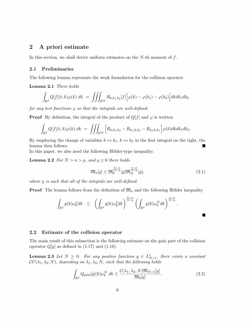
2 A priori estimate
In this section, we shall derive uniform estimates on the N -th moment of f .
2.1 Preliminaries
The following lemma represents the weak formulation for the collision operator
Lemma 2.1 There holds∫RdQ[f ](t, k)ϕ(k) dk =
∫∫∫R3d
Rk,k1,k2 [f ][ϕ(k)− ϕ(k1)− ϕ(k2)
]dkdk1dk2
for any test functions ϕ so that the integrals are well-defined.
Proof By definition, the integral of the product of Q[f ] and ϕ is written∫RdQ[f ](t, k)ϕ(k) dk =
∫∫∫R3d
[Rk,k1,k2 −Rk1,k,k2 −Rk2,k,k1
]ϕ(k)dkdk1dk2.
By employing the change of variables k ↔ k1, k ↔ k2 in the first integral on the right, thelemma then follows.In this paper, we also need the following Holder-type inequality.
Lemma 2.2 For N > n > p, and g ≥ 0 there holds
Mn[g] ≤MN−nN−pp [g]M
n−pN−pN [g], (2.1)
where g is such that all of the integrals are well-defined.
Proof The lemma follows from the definition of Mn and the following Holder inequality∫Rdg(k)ωnkdk ≤
(∫Rdg(k)ωpkdk
)N−nN−p
(∫Rdg(k)ωNk dk
) n−pN−p
.
2.2 Estimate of the collision operator
The main result of this subsection is the following estimate on the gain part of the collisionoperator Q[g] as defined in (1.17) and (1.18).
Lemma 2.3 Let N ≥ 0. For any positive function g ∈ L1N+1, there exists a constant
CC(λ1, λ2, N), depending on λ1, λ2, N , such that the following holds∫RdQgain[g](k)ωNk dk ≤ C(λ1, λ2, N)MN+1[g]
M0[g]. (2.2)
9
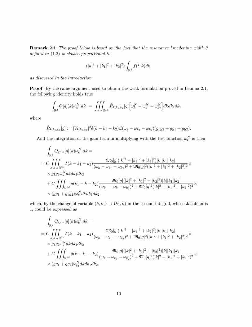
Remark 2.1 The proof below is based on the fact that the resonance broadening width θdefined in (1.2) is chosen proportional to
(|k|2 + |k1|2 + |k2|2)
∫R3
f(t, k)dk,
as discussed in the introduction.
Proof By the same argument used to obtain the weak formulation proved in Lemma 2.1,the following identity holds true∫
RdQ[g](k)ωNk dk =
∫∫∫R3d
Rk,k1,k2 [g][ωNk − ωNk1 − ω
Nk2
]dkdk1dk2,
where
Rk,k1,k2 [g] := |Vk,k1,k2 |2δ(k − k1 − k2)L(ωk − ωk1 − ωk2)(g1g2 + gg1 + gg2).
And the integration of the gain term in multiplying with the test function ωNk is then∫RdQgain[g](k)ωNk dk =
= C
∫∫∫R3d
δ(k − k1 − k2)M0[g](|k|2 + |k1|2 + |k2|2)|k||k1||k2|
(ωk − ωk1 − ωk2)2 + M0[g]2(|k|2 + |k1|2 + |k2|2)2×
× g1g2ωNk dkdk1dk2
+ C
∫∫∫R3d
δ(k1 − k − k2)M0[g](|k|2 + |k1|2 + |k2|2)|k||k1||k2|
(ωk1 − ωk − ωk2)2 + M0[g]2(|k|2 + |k1|2 + |k2|2)2×
× (gg1 + g1g2)ωNk dkdk1dk2,
which, by the change of variable (k, k1)→ (k1, k) in the second integral, whose Jacobian is1, could be expressed as∫
RdQgain[g](k)ωNk dk =
= C
∫∫∫R3d
δ(k − k1 − k2)M0[g](|k|2 + |k1|2 + |k2|2)|k||k1||k2|
(ωk − ωk1 − ωk2)2 + M0[g]2(|k|2 + |k1|2 + |k2|2)2×
× g1g2ωNk dkdk1dk2
+ C
∫∫∫R3d
δ(k − k1 − k2)M0[g](|k|2 + |k1|2 + |k2|2)|k||k1||k2|
(ωk − ωk1 − ωk2)2 + M0[g]2(|k|2 + |k1|2 + |k2|2)2×
× (gg1 + gg2)ωNk1dkdk1dk2.
10

By the symmetry of k1 and k2 in the second integral,∫RdQgain[g](k)ωNk dk =
= C
∫∫∫R3d
δ(k − k1 − k2)M0[g](|k|2 + |k1|2 + |k2|2)|k||k1||k2|
(ωk − ωk1 − ωk2)2 + M0[g]2(|k|2 + |k1|2 + |k2|2)2×
× g1g2ωNk dkdk1dk2
+ C
∫∫∫R3d
δ(k − k1 − k2)M0[g](|k|2 + |k1|2 + |k2|2)|k||k1||k2|
(ωk − ωk1 − ωk2)2 + M0[g]2(|k|2 + |k1|2 + |k2|2)2×
× gg1
[ωNk1 + ωNk2
]dkdk1dk2.
Let us now look at the fractional term in the above integral
K :=M0[g](|k|2 + |k1|2 + |k2|2)|k||k1||k2|
(ωk − ωk1 − ωk2)2 + M0[g]2(|k|2 + |k1|2 + |k2|2)2.
Since the denominator (ωk−ωk1−ωk2)2+M20(|k|2+|k1|2+|k2|2)2 is greater than M0[g]2(|k|2+
|k1|2 + |k2|2)2, the whole fraction can be bounded as
K ≤ |k||k1||k2|M0[g](|k|2 + |k1|2 + |k2|2)
,
which leads to the following∫RdQgain[g](k)ωNk dk
≤ C
∫∫∫R3d
δ(k − k1 − k2)|k||k1||k2|
M0[g](|k|2 + |k1|2 + |k2|2)g1g2ω
Nk dkdk1dk2
+ C
∫∫∫R3d
δ(k − k1 − k2)|k||k1||k2|
M0[g](|k|2 + |k1|2 + |k2|2)gg1
[ωNk1 + ωNk2
]dkdk1dk2,
which can be rewritten in the following equivalent form, with the right hand side being thesum of I1 and I2 ∫
RdQgain[g](k)ωNk dk ≤ I1 + I2, (2.3)
where
I1 := C
∫∫∫R3d
δ(k − k1 − k2)|k||k1||k2|
M0[g](|k|2 + |k1|2 + |k2|2)g1g2ω
Nk dkdk1dk2
I2 := C
∫∫∫R3d
δ(k − k1 − k2)|k||k1||k2|
M0[g](|k|2 + |k1|2 + |k2|2)gg1
[ωNk1 + ωNk2
]dkdk1dk2.
(2.4)
Let us first estimate I1. By the resonant condition k = k1 + k2, we have
ωk =√λ1 + λ2|k|2 ≤
√λ1 + λ2(|k1|+ |k2|)2 < 2
√λ1 + λ2|k1|2+2
√λ1 + λ2|k2|2 = 2ωk1+2ωk2 ,
11

which, thanks to the Cauchy-Schwarz inequality, leads to
ωNk ≤ C(λ1, λ2, N)(ωNk1 + ωNk2),
where C(λ1, λ2, N) is some constant depending on λ1, λ2, N .Thus, we obtain
I1 ≤ C(λ1, λ2, N)
∫∫∫R3d
δ(k − k1 − k2)|k||k1||k2|
M0[g](|k|2 + |k1|2 + |k2|2)g1g2
[ωNk1 + ωNk2
]dkdk1dk2.
Taking into account the definition of the Dirac function δ(k − k1 − k2) the above integralon R3d can be reduced to an integral on R2d only
I1 ≤ C(λ1, λ2, N)
∫∫R2d
|k1 + k2||k1||k2|M0[g](|k|2 + |k1|2 + |k2|2)
g1g2
[ωNk1 + ωNk2
]dk1dk2.
Due to the inequality |k1 + k2|2 + |k1|2 + |k2|2 ≥ 2|k1||k2|, the kernel of the above integralcan be bounded as
|k1 + k2||k1||k2||k1 + k2|2 + |k1|2 + |k2|2
≤ |k1 + k2|2
≤ |k1|+ |k2|2
,
yielding
I1 ≤C(λ1, λ2, N)
M0[g]
∫∫R2d
(|k1|+ |k2|)g1g2
[ωNk1 + ωNk2
]dk1dk2.
Observing that
|k1| ≤ωk1√λ2, |k2| ≤
ωk2√λ2,
we can bound
(|k1|+ |k2|)[ωNk1 + ωNk2
]≤ C(ωk1 + ωk2)
[ωNk1 + ωNk2
]≤ C
[ωN+1k1
+ ωN+1k2
],
which yields the following estimate on I1 in terms of the functional defined in (1.21)
I1 ≤C(λ1, λ2, N)
M0[g]
∫∫R2d
g1g2
[ωN+1k1
+ ωN+1k2
]dk1dk2
≤ C
M0[g]MN+1[g].
(2.5)
Let us now estimate I2. Using the resonant condition k2 = k − k1, we obtain the followingrelation between ωk2 and ωk, ωk1
ωk2 =√λ1 + λ2|k2|2 <
√λ1 + λ2(|k1|+ |k|)2 ≤ 2
√λ1 + λ2|k|2+2
√λ1 + λ2|k1|2 = 2ωk+2ωk1 ,
which, by the Cauchy-Schwarz inequality, leads to
ωNk2 ≤ C(λ1, λ2, N)(ωNk + ωNk1),
12
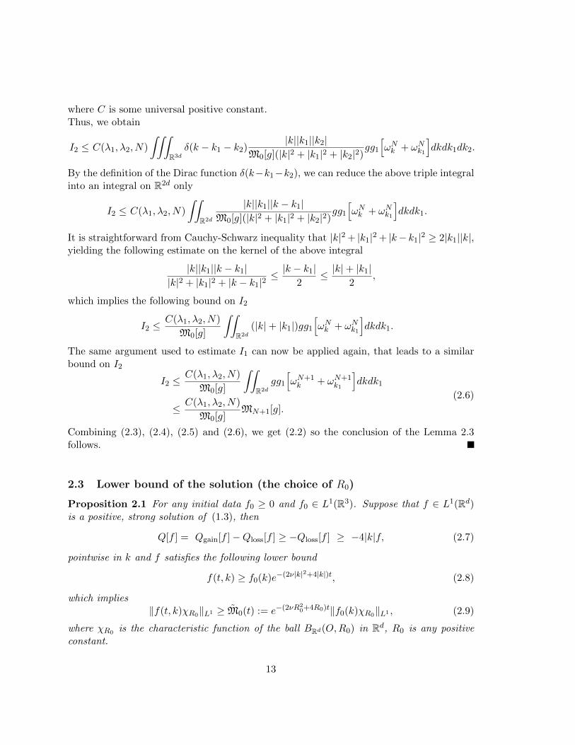
where C is some universal positive constant.Thus, we obtain
I2 ≤ C(λ1, λ2, N)
∫∫∫R3d
δ(k − k1 − k2)|k||k1||k2|
M0[g](|k|2 + |k1|2 + |k2|2)gg1
[ωNk + ωNk1
]dkdk1dk2.
By the definition of the Dirac function δ(k−k1−k2), we can reduce the above triple integralinto an integral on R2d only
I2 ≤ C(λ1, λ2, N)
∫∫R2d
|k||k1||k − k1|M0[g](|k|2 + |k1|2 + |k2|2)
gg1
[ωNk + ωNk1
]dkdk1.
It is straightforward from Cauchy-Schwarz inequality that |k|2 + |k1|2 + |k− k1|2 ≥ 2|k1||k|,yielding the following estimate on the kernel of the above integral
|k||k1||k − k1||k|2 + |k1|2 + |k − k1|2
≤ |k − k1|2
≤ |k|+ |k1|2
,
which implies the following bound on I2
I2 ≤C(λ1, λ2, N)
M0[g]
∫∫R2d
(|k|+ |k1|)gg1
[ωNk + ωNk1
]dkdk1.
The same argument used to estimate I1 can now be applied again, that leads to a similarbound on I2
I2 ≤C(λ1, λ2, N)
M0[g]
∫∫R2d
gg1
[ωN+1k + ωN+1
k1
]dkdk1
≤ C(λ1, λ2, N)
M0[g]MN+1[g].
(2.6)
Combining (2.3), (2.4), (2.5) and (2.6), we get (2.2) so the conclusion of the Lemma 2.3follows.
2.3 Lower bound of the solution (the choice of R0)
Proposition 2.1 For any initial data f0 ≥ 0 and f0 ∈ L1(R3). Suppose that f ∈ L1(Rd)is a positive, strong solution of (1.3), then
Q[f ] = Qgain[f ]−Qloss[f ] ≥ −Qloss[f ] ≥ −4|k|f, (2.7)
pointwise in k and f satisfies the following lower bound
f(t, k) ≥ f0(k)e−(2ν|k|2+4|k|)t, (2.8)
which implies‖f(t, k)χR0‖L1 ≥ M0(t) := e−(2νR2
0+4R0)t‖f0(k)χR0‖L1 , (2.9)
where χR0 is the characteristic function of the ball BRd(O,R0) in Rd, R0 is any positiveconstant.
13

Proof Let us first recall the formulation of Q[f ]
Q[f ] =
∫∫Rd×Rd
|Vk,k1,k2 |2δ(k − k1 − k2)Lf (ωk − ωk1 − ωk2)(f1f2 − 2ff1)dk1dk2
+ 2
∫∫Rd×Rd
|Vk1,k,k2 |2δ(k1 − k − k2)Lf (ωk1 − ωk − ωk2)(−ff2 + ff1 + f1f2)dk1dk2.
and in order to get (2.8), we will work with
Q[f ] = Qgain[f ] − Qloss[f ],
where the formulation of Qloss[f ]
−Qloss[f ] = − 2f
∫Rd×Rd
|Vk,k1,k2 |2δ(k − k1 − k2)Lf (ωk − ωk1 − ωk2)f1dk1dk2
− 2f
∫Rd×Rd
|Vk1,k,k2 |2δ(k1 − k − k2)Lf (ωk1 − ωk − ωk2)f2dk1dk2
=: − I1 − I2.
(2.10)
In order to get the lower bound (2.7), we discard the gain operator defined in (1.18) andestimate from below the loss part.
Let us estimate the double integral I1, which can be reduced to an integral on Rd bytaking into account the definition of δ(k − k1 − k2) as follows
I1 := 2f
∫Rd|Vk,k1,k−k1 |2Lf (ωk − ωk1 − ωk−k1)f1dk1.
By the definition of Vk,k1,k−k1 , Lf (ωk − ωk1 − ωk−k1), Γk,k1,k2 , and the inequality
(ωk − ωk1 − ωk−k1)2 + Γ2k,k1,k−k1 ≥ Γ2
k,k1,k−k1 ,
we obtain the following inequality on the kernel of I1
|Vk,k1,k−k1 |2Lf (ωk − ωk1 − ωk−k1) =|k||k1||k − k1|Γk,k1,k−k1
(ωk − ωk1 − ωk−k1)2 + Γ2k,k1,k−k1
≤ |k||k1||k − k1|Γk,k1,k−k1
≤ |k||k1||k − k1|M0[f ](|k|2 + |k1|2 + |k − k1|2)
.
By the positivity of |k|2 and the Cauchy-Schwarz inequality, the following holds true
|k|2 + |k1|2 + |k − k1|2 ≥ |k1|2 + |k − k1|2 ≥ 2|k1||k − k1|,
which implies
|Vk,k1,k−k1 |2Lf (ωk − ωk1 − ωk−k1) ≤ 2|k|M0[f ]
.
14

As a result, we have the following estimate on I1
I1 ≤2|k|f
∫Rd f1dk1
M0[f ]≤ 2|k|f. (2.11)
I2 can be estimated in a similar way. We can reduce I2 to an integral on Rd by taking intoaccount the definition of δ(k1 − k − k2) as follows
I2 := f
∫Rd|Vk+k2,k,k2 |2Lf (ωk+k2 − ωk − ωk2)f2dk2.
Taking into account the definite of Vk+k2,k,k2 , Lf (ωk+k2 − ωk − ωk2), Γk+k2,k,k2 , and theinequality
(ωk+k2 − ωk − ωk2)2 + Γ2k+k2,k,k2 ≥ Γ2
k+k2,k,k2 ,
the following estimate on the kernel of I2 can be obtained
|Vk+k2,k,k2 |2Lf (ωk+k2 − ωk − ωk2) =|k + k2||k||k2|Γk+k2,k,k2
(ωk+k2 − ωk − ωk2)2 + Γ2k+k2,k,k2
≤ |k + k2||k||k2|M0[f ](|k + k2|2 + |k|2 + |k2|2)
.
Using the positivity of |k|2 and the Cauchy-Schwarz inequality, we find
|k + k2|2 + |k|2 + |k2|2 ≥ |k + k2|2 + |k2|2 ≥ 2|k + k2||k2|,
which implies
|Vk+k2,k,k2 |2Lf (ωk+k2 − ωk − ωk2) ≤ 2|k|M0[f ]
.
We then obtain the following estimate on I2
I2 ≤2|k|f
∫Rd f2dk2
M0[f ]= 2|k|f. (2.12)
Combining (2.10), (2.11) and (2.12) yields
Q[f ] ≥ − 4|k|f. (2.13)
By plugging the above inequality into (1.3), we obtain a differential inequality on f
∂tf −Q[f ]− 2ν|k|2f ≥ ∂tf + (2ν|k|2 + 4|k|)f ≥ 0.
A Gronwall inequality argument applied to the above differential inequality leads to
f(t, k) ≥ f0(k)e−(2ν|k|2+4|k|)t,
and so (2.8) holds.
15

Multiplying both sides of the above inequality with χR0 is the characteristic function ofthe ball BRd(O,R0) in Rd, and taking the integral with respect to k on Rd, yield
‖fχR0‖1 ≥∫RdχR0f(t, k)dk ≥
∫RdχR0f0(k)e−(2ν|k|2+4|k|)tdk
≥ e−(2νR20+4R0)t
∫RdχR0f0(k)dk ≥ ‖f0χR0‖1,
and so (2.9) holds true. The proof of Proposition 2.1 is completed.
2.4 Weighted L1N (N ≥ 0) estimates
For a given function g, let us recall the N -th moment of g
MN [g] =
∫RdωNk g(k)dk.
Proposition 2.2 Let N ≥ 0. Suppose that f0(k) is a nonnegative initial data satisfying∫Rdf0(k)ωNk dk <∞,
and that nonnegative solutions f(t, k) of (1.3) satisfies
M0[f ](t) ≥ M0(t) = e−(2νR20+4R0)t‖f0(k)χR0‖L1 > 0,
where M0(t) is the quantity considered in Proposition 2.1.Then, there exists a positive constant C0(λ1, λ2) is a constant depending on λ1, λ2 and
independent of N such that
MN+1[Q[f ]](t)− 2νMN [|k|2f ](t) =
=
∫RdQ[f ](t, k)ωN+1
k dk − 2ν
∫Rd|k|2f(t, k)ωNk dk
≤ C0(λ1, λ2)
(1 +
e(4νR20+8R0)t
‖f0(k)χR0‖2L1
)∫Rdf(t, k)ωNk dk,
(2.14)
which implies that nonnegative solutions f(t, k) of (1.3), with f(0, k) = f0(k), satisfy
MN [f ](t) =
∫Rdf(t, k)ωNk dk ≤ e
C(λ1,λ2)
(t+ e
(4νR20+8R0)t
(4νR20+8R0)‖f0(k)χR0
‖2L1
) ∫Rdf0(k)ωNk dk,
(2.15)where C(λ1, λ2) is a constant depending on λ1, λ2.
16
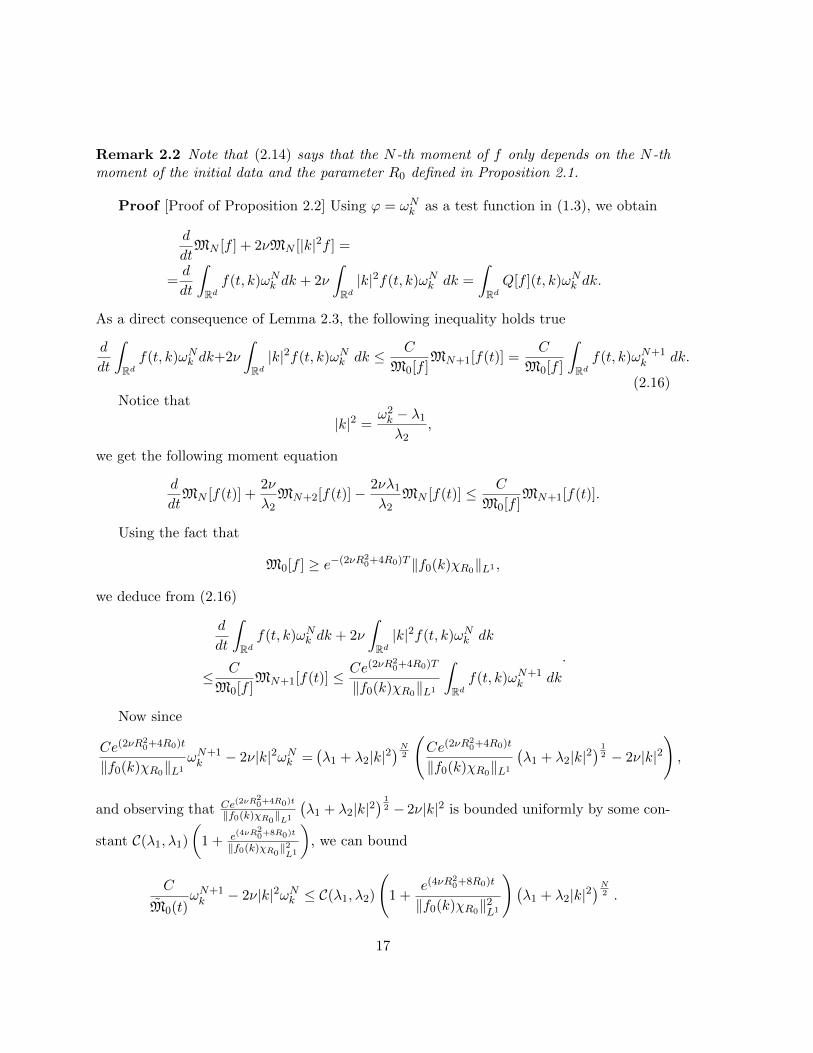
Remark 2.2 Note that (2.14) says that the N -th moment of f only depends on the N -thmoment of the initial data and the parameter R0 defined in Proposition 2.1.
Proof [Proof of Proposition 2.2] Using ϕ = ωNk as a test function in (1.3), we obtain
d
dtMN [f ] + 2νMN [|k|2f ] =
=d
dt
∫Rdf(t, k)ωNk dk + 2ν
∫Rd|k|2f(t, k)ωNk dk =
∫RdQ[f ](t, k)ωNk dk.
As a direct consequence of Lemma 2.3, the following inequality holds true
d
dt
∫Rdf(t, k)ωNk dk+2ν
∫Rd|k|2f(t, k)ωNk dk ≤ C
M0[f ]MN+1[f(t)] =
C
M0[f ]
∫Rdf(t, k)ωN+1
k dk.
(2.16)Notice that
|k|2 =ω2k − λ1
λ2,
we get the following moment equation
d
dtMN [f(t)] +
2ν
λ2MN+2[f(t)]− 2νλ1
λ2MN [f(t)] ≤ C
M0[f ]MN+1[f(t)].
Using the fact that
M0[f ] ≥ e−(2νR20+4R0)T ‖f0(k)χR0‖L1 ,
we deduce from (2.16)
d
dt
∫Rdf(t, k)ωNk dk + 2ν
∫Rd|k|2f(t, k)ωNk dk
≤ C
M0[f ]MN+1[f(t)] ≤ Ce(2νR2
0+4R0)T
‖f0(k)χR0‖L1
∫Rdf(t, k)ωN+1
k dk
.
Now since
Ce(2νR20+4R0)t
‖f0(k)χR0‖L1
ωN+1k − 2ν|k|2ωNk =
(λ1 + λ2|k|2
)N2
(Ce(2νR2
0+4R0)t
‖f0(k)χR0‖L1
(λ1 + λ2|k|2
) 12 − 2ν|k|2
),
and observing that Ce(2νR20+4R0)t
‖f0(k)χR0‖L1
(λ1 + λ2|k|2
) 12 − 2ν|k|2 is bounded uniformly by some con-
stant C(λ1, λ1)
(1 + e(4νR
20+8R0)t
‖f0(k)χR0‖2L1
), we can bound
C
M0(t)ωN+1k − 2ν|k|2ωNk ≤ C(λ1, λ2)
(1 +
e(4νR20+8R0)t
‖f0(k)χR0‖2L1
)(λ1 + λ2|k|2
)N2 .
17
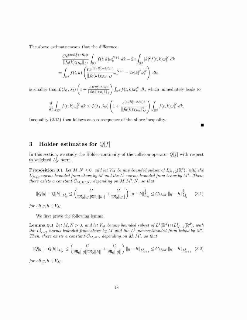
The above estimate means that the difference
Ce(2νR20+4R0)t
‖f0(k)χR0‖L1
∫Rdf(t, k)ωN+1
k dk − 2ν
∫Rd|k|2f(t, k)ωNk dk
=
∫Rdf(t, k)
(Ce(2νR2
0+4R0)t
‖f0(k)χR0‖L1
ωN+1k − 2ν|k|2ωNk
)dk,
is smaller than C(λ1, λ2)
(1 + e(4νR
20+8R0)t
‖f0(k)χR0‖2L1
)∫Rd f(t, k)ωNk dk, which immediately leads to
d
dt
∫Rdf(t, k)ωNk dk ≤ C(λ1, λ2)
(1 +
e(4νR20+8R0)t
‖f0(k)χR0‖2L1
)∫Rdf(t, k)ωNk dk.
Inequality (2.15) then follows as a consequence of the above inequality.
3 Holder estimates for Q[f ]
In this section, we study the Holder continuity of the collision operator Q[f ] with respectto weighted L1
N norm.
Proposition 3.1 Let M,N ≥ 0, and let VM be any bounded subset of L1N+2(Rd), with the
L1N+2 norms bounded from above by M and the L1 norms bounded from below by M ′. Then,
there exists a constant CM,M ′,N , depending on M,M ′, N , so that
‖Q[g]−Q[h]‖L1N≤(
C
M0[|g|]M0[|h|]+
C
M0[|g|]
)‖g − h‖
12
L1N≤ CM,M ′‖g − h‖
12
L1N
(3.1)
for all g, h ∈ VM .
We first prove the following lemma.
Lemma 3.1 Let M,N > 0, and let VM be any bounded subset of L1(Rd)∩L1N+1(Rd), with
the L1N+2 norms bounded from above by M and the L1 norms bounded from below by M ′.
Then, there exists a constant CM,M ′, depending on M,M ′, so that
‖Q[g]−Q[h]‖L1N≤(
C
M0[|g|]M0[|h|]+
C
M0[|g|]
)‖g − h‖L1
N+1≤ CM,M ′‖g − h‖L1
N+1(3.2)
for all g, h ∈ VM .
18

Proof We first compute the difference between Q[g] and Q[h]
Q[g]−Q[h] =
∫∫R2d
[Rk,k1,k2 [g]−Rk,k1,k2 [h]− 2(Rk1,k,k2 [g]−Rk1,k,k2 [h])
]dk1dk2,
whose L1N -norm is
‖Q[g]−Q[h]‖L1N
=
∫RdωNk |Q[g](k)−Q[h](k)|dk
≤∫∫∫
R3d
ωNk |Rk,k1,k2 [g]−Rk,k1,k2 [h]| dkdk1dk2
+ 2
∫∫∫R3d
ωNk |Rk1,k,k2 [g]−Rk1,k,k2 [h]|dkdk1dk2
=
∫∫∫R3d
|Rk,k1,k2 [g]−Rk,k1,k2 [h]|(ωNk + ωNk1 + ωNk2
)dkdk1dk2.
Recalling that
Rk,k1,k2 [g] = C|Vk,k1,k2 |2δ(k − k1 − k2)Lg(ωk − ωk1 − ωk2)(g1g2 − gg1 − gg2),
we find the following estimate on ‖Q[g]−Q[h]‖L1N
‖Q[g]−Q[h]‖L1N≤ J1 + J2, (3.3)
where
J1 :=
∫∫∫R3d
|Vk,k1,k2 |2δ(k − k1 − k2)∣∣∣Lg(ωk − ωk1 − ωk2)g1g2
− Lh(ωk − ωk1 − ωk2)h1h2
∣∣∣(ωNk + ωNk1 + ωNk2
)dkdk1dk2,
J2 :=2
∫∫∫R3d
|Vk1,k,k2 |2δ(k1 − k − k2)∣∣∣Lg(ωk1 − ωk − ωk2)gg2
− Lh(ωk1 − ωk − ωk2)hh2
∣∣∣(ωNk + ωNk1 + ωNk2
)dkdk1dk2.
(3.4)
Let us now split the proof into two steps.Step 1: Estimating J1. Define the quantity inside the triple integral of J1 after dropping(ωNk + ωNk1 + ωNk2
)to be J1
J1 := |Vk,k1,k2 |2δ(k − k1 − k2)∣∣∣Lg(ωk − ωk1 − ωk2)g1g2 − Lh(ωk − ωk1 − ωk2)h1h2
∣∣∣,which, by the triangle inequality, can be bounded as
J1 ≤ |Vk,k1,k2 |2δ(k − k1 − k2)Lg(ωk − ωk1 − ωk2)|g1g2 − h1h2|
+ |Vk,k1,k2 |2δ(k − k1 − k2)∣∣∣Lg(ωk − ωk1 − ωk2)− Lh(ωk − ωk1 − ωk2)
∣∣∣|h1h2|.
19

Define the two terms on the right hand side of the above inequality to be J11 and J12,respectively.Let us now study J11 in details. Using the definition of Lg and the triangle inequality
|g1g2 − h1h2| ≤ |g1||g2 − h2|+ |h2||g1 − h1|,
yields the following estimate on J11
J11 ≤ C|k||k1||k2|δ(k − k1 − k2)Γg,k,k1,k2
(ωk − ωk1 − ωk2)2 + Γ2g,k,k1,k2
|g1||g2 − h2|
+ C|k||k1||k2|δ(k − k1 − k2)Γg,k,k1,k2
(ωk − ωk1 − ωk2)2 + Γ2g,k,k1,k2
|h2||g1 − h1|.
By the inequality(ωk − ωk1 − ωk2)2 + Γ2
g,k,k1,k2 ≥ Γ2g,k,k1,k2 ,
we can bound J11 as
J11 ≤ C|k||k1||k2|δ(k − k1 − k2)1
Γg,k,k1,k2|g1||g2 − h2|
+ C|k||k1||k2|δ(k − k1 − k2)1
Γg,k,k1,k2|h2||g1 − h1|.
The right hand side of the above inequality can be estimated by employing the followingCauchy-Schwarz inequality
Γg,k,k1,k2 = M0[|g|](|k|2 + |k1|2 + |k2|2
)≥M0[|g|]
(|k1|2 + |k2|2
)≥ 2M0[|g|]|k1||k2|,
where we have just used the lower bound of M0[|g|], yielding
J11 ≤C
M0[|g|]|k|δ(k − k1 − k2)|g1||g2 − h2|+
C
M0[|g|]|k|δ(k − k1 − k2)|h2||g1 − h1|.
Multiplying the above inequality with(ωNk + ωNk1 + ωNk2
)and integrating in k, k1 and k2
lead to∫∫∫R3d
J11
(ωNk + ωNk1 + ωNk2
)dkdk1dk2
≤∫∫∫
R3d
C
M0[|g|]||k|δ(k − k1 − k2) [|g1||g2 − h2|+ |h2||g1 − h1|]
(ωNk + ωNk1 + ωNk2
)dkdk1dk2.
Using the resonant condition k = k1 + k2, we reduce the triple integral on the right handside to a double integral∫∫∫
R3
J11
(ωNk + ωNk1 + ωNk2
)dkdk1dk2
≤ C
M0[|g|]
∫∫R2d
|k1 + k2| [|g1||g2 − h2|+ |h2||g1 − h1|](ωNk1 + ωNk2
)dk1dk2,
20

where, we have just used the inequality
ωNk1+k2 ≤ CωNk1 + CωNk2 ,
proved in Proposition 2.3, to bound the sum ωNk + ωNk1 + ωNk2 by C(ωNk1 + ωNk2
).
Observing that
|k1 + k2|(ωNk1 + ωNk2
)≤ (|k1|+ |k2|)
(ωNk1 + ωNk2
)≤ C
(ωN+1k1
+ ωN+1k2
),
we find ∫∫∫R3d
J11
(ωNk + ωNk1 + ωNk2
)dkdk1dk2
≤ C
M0[|g|]
∫∫R2d
[|g1||g2 − h2|+ |h2||g1 − h1|](ωN+1k1
+ ωN+1k2
)dk1dk2,
which immediately leads to∫∫∫R3d
J11
(ωNk + ωNk1 + ωNk2
)dkdk1dk2
≤ C
M0[|g|]‖g − h‖L1
N+1
(‖g‖L1 + ‖g‖L1
N+1+ ‖h‖L1 + ‖h‖L1
N+1
)≤ C
M0[|g|]‖g − h‖L1
N+1
(‖g‖L1
N+1+ ‖h‖L1
N+1
).
(3.5)
Now, let us look at J12, which can be written as
J12 = C|k||k1||k2|δ(k − k1 − k2)|h1h2|×
×
∣∣∣∣∣Γg,k,k1,k2 [(ωk − ωk1 − ωk2)2 + Γ2h,k,k1,k2
]− Γh,k,k1,k2 [(ωk − ωk1 − ωk2)2 + Γ2g,k,k1,k2
]
[(ωk − ωk1 − ωk2)2 + Γ2g,k,k1,k2
][(ωk − ωk1 − ωk2)2 + Γ2h,k,k1,k2
]
∣∣∣∣∣= C|k||k1||k2|δ(k − k1 − k2)|h1h2|×
×|(ωk − ωk1 − ωk2)2 − Γg,k,k1,k2Γh,k,k1,k2 ||Γg,k,k1,k2 − Γh,k,k1,k2 |[(ωk − ωk1 − ωk2)2 + Γ2
g,k,k1,k2][(ωk − ωk1 − ωk2)2 + Γ2
h,k,k1,k2]
It follows from the Cauchy-Schwarz inequality that
[(ωk − ωk1 − ωk2)2 + Γ2g,k,k1,k2 ][(ωk − ωk1 − ωk2)2 + Γ2
h,k,k1,k2 ]
≥ |(ωk − ωk1 − ωk2)2 − Γg,k,k1,k2Γh,k,k1,k2 ||(ωk − ωk1 − ωk2)2 + Γg,k,k1,k2Γh,k,k1,k2 |≥ |(ωk − ωk1 − ωk2)2 − Γg,k,k1,k2Γh,k,k1,k2 |Γg,k,k1,k2Γh,k,k1,k2 ,
from which, we obtain the following estimate on J12
J12 ≤ C|k||k1||k2||h1h2|δ(k − k1 − k2)|Γg,k,k1,k2 − Γh,k,k1,k2 |
Γg,k,k1,k2Γh,k,k1,k2.
21

The numerator of the fraction on the right hand side has the following interesting property
|Γg,k,k1,k2 − Γh,k,k1,k2 | = C∣∣(k2 + k2
1 + k22)M0[|g| − |h|]
∣∣ ,which can be bounded as follows
|Γg,k,k1,k2 − Γh,k,k1,k2 | ≤ C(k2 + k21 + k2
2)‖g − h‖L1 ,
yielding an upper bound on J12
J12 ≤ C|k||k1||k2||h1h2|δ(k − k1 − k2)‖g − h‖L1 ,
(k2 + k21 + k2
2)M0[|g|]M0[|h|].
By the Cauchy-Schwarz inequality
k2 + k21 + k2
2 ≥ k21 + k2
2 ≥ 2|k1||k2|,
and the lower bound on M0[|g|] and M0[|h|], the following estimate on J12 then follows
J12 ≤C
M0[|g|]M0[|h|]||k||h1h2|δ(k − k1 − k2)‖g − h‖L1 .
Multiplying the above inequality with(ωNk + ωNk1 + ωNk2
)and integrate in k, k1 and k2, the
same argument used to deduce (3.5) leads to∫∫∫R3d
J12
(ωNk + ωNk1 + ωNk2
)dkdk1dk2 ≤
C
M0[|g|]M0[|h|]‖g − h‖L1
N+1. (3.6)
Note that C is a constant depending on(‖g‖L1
N+1+ ‖h‖L1
N+1
). Combining (3.5) and (3.6)
yields
J1 ≤(
C
M0[|g|]M0[|h|]+
C
M0[|g|]
)‖g − h‖L1
N+1, (3.7)
where C is a constant depending on(‖g‖L1
N+1+ ‖h‖L1
N+1
).
Step 2: Estimating J2. The proof of estimating J2 follows exactly the same argumentused in Step 1. As a consequence, we omit some details and give only the main estimatesin the sequel. First, define the quantity inside the triple integral of J2 after dropping(ωNk + ωNk1 + ωNk2
)to be J2
J2 := |Vk1,k,k2 |2δ(k1 − k − k2)∣∣∣Lg(ωk1 − ωk − ωk2)gg2 − Lh(ωk1 − ωk − ωk2)hh2
∣∣∣,which, by the triangle inequality, can be bounded as
J2 ≤ |Vk1,k,k2 |2δ(k1 − k − k2)Lg(ωk1 − ωk − ωk2)|gg2 − hh2|
+ |Vk1,k,k2 |2δ(k1 − k − k2)∣∣∣Lg(ωk1 − ωk − ωk2)− Lh(ωk1 − ωk − ωk2)
∣∣∣|hh2|.
22
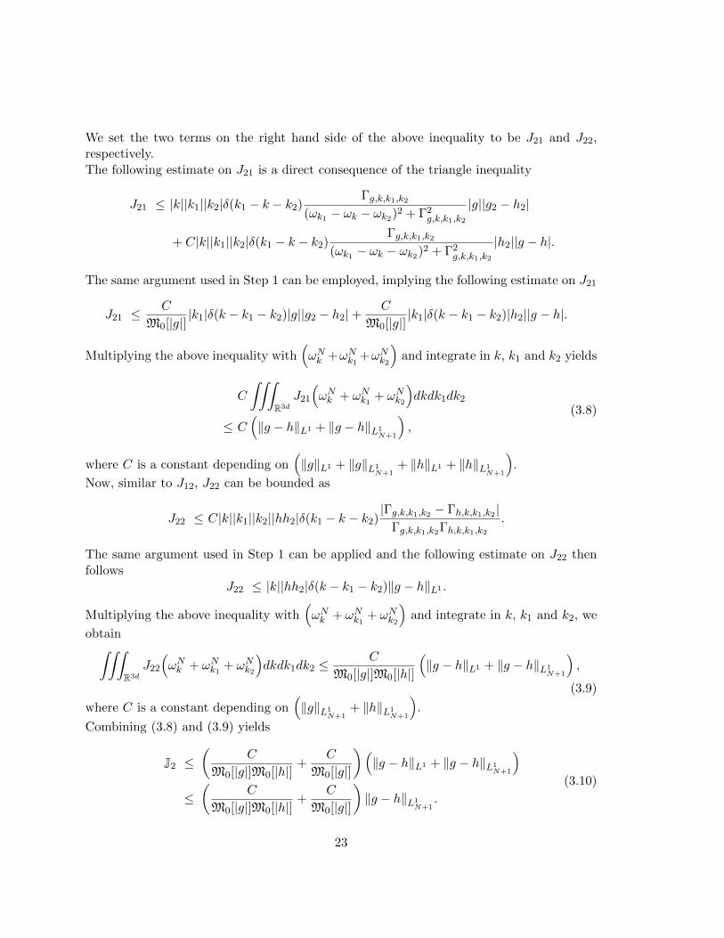
We set the two terms on the right hand side of the above inequality to be J21 and J22,respectively.The following estimate on J21 is a direct consequence of the triangle inequality
J21 ≤ |k||k1||k2|δ(k1 − k − k2)Γg,k,k1,k2
(ωk1 − ωk − ωk2)2 + Γ2g,k,k1,k2
|g||g2 − h2|
+ C|k||k1||k2|δ(k1 − k − k2)Γg,k,k1,k2
(ωk1 − ωk − ωk2)2 + Γ2g,k,k1,k2
|h2||g − h|.
The same argument used in Step 1 can be employed, implying the following estimate on J21
J21 ≤C
M0[|g|]|k1|δ(k − k1 − k2)|g||g2 − h2|+
C
M0[|g|]|k1|δ(k − k1 − k2)|h2||g − h|.
Multiplying the above inequality with(ωNk +ωNk1 +ωNk2
)and integrate in k, k1 and k2 yields
C
∫∫∫R3d
J21
(ωNk + ωNk1 + ωNk2
)dkdk1dk2
≤ C(‖g − h‖L1 + ‖g − h‖L1
N+1
),
(3.8)
where C is a constant depending on(‖g‖L1 + ‖g‖L1
N+1+ ‖h‖L1 + ‖h‖L1
N+1
).
Now, similar to J12, J22 can be bounded as
J22 ≤ C|k||k1||k2||hh2|δ(k1 − k − k2)|Γg,k,k1,k2 − Γh,k,k1,k2 |
Γg,k,k1,k2Γh,k,k1,k2.
The same argument used in Step 1 can be applied and the following estimate on J22 thenfollows
J22 ≤ |k||hh2|δ(k − k1 − k2)‖g − h‖L1 .
Multiplying the above inequality with(ωNk + ωNk1 + ωNk2
)and integrate in k, k1 and k2, we
obtain∫∫∫R3d
J22
(ωNk + ωNk1 + ωNk2
)dkdk1dk2 ≤
C
M0[|g|]M0[|h|]
(‖g − h‖L1 + ‖g − h‖L1
N+1
),
(3.9)
where C is a constant depending on(‖g‖L1
N+1+ ‖h‖L1
N+1
).
Combining (3.8) and (3.9) yields
J2 ≤(
C
M0[|g|]M0[|h|]+
C
M0[|g|]
)(‖g − h‖L1 + ‖g − h‖L1
N+1
)≤(
C
M0[|g|]M0[|h|]+
C
M0[|g|]
)‖g − h‖L1
N+1.
(3.10)
23

Putting the two estimates (3.7) and (3.10) together with (3.3) and (3.4), the conclusion ofthe Lemma then follows.Proof [Proof of Proposition 3.1] The proposition now follows straightforwardly from theprevious lemma. Indeed, we recall the interpolation inequality (see Lemma 2.2):
‖g‖L1n≤ ‖g‖
q−nq−pL1p‖g‖
n−pq−pL1q
for q > n > p. Together with the boundedness of g, h in L11 ∩ L1
N+2, we obtain
‖g − h‖L1N+1≤ ‖g − h‖
12
L1N‖g − h‖
12
L1N+2≤ CM‖g − h‖
12
L1N
Lemma 3.1 yields
‖Q[g]−Q[h]‖L1N≤ CM,M ′,N‖g − h‖
12
L1N
which holds for all N ≥ 0. The proposition follows.
4 Proof of Theorem 1.1
We shall apply Theorem 1.2 for (1.3), which reads
∂tf = Q[f ], Q[f ] := Q[f ]− 2ν|k|2f.
Fix an N > 1. We choose the Banach spaces E = L1N
(Rd), F = L1
N+3
(Rd), endowed
with the norms‖f‖E := ‖f‖L1
N, ‖f‖∗ := ‖f‖L1
N+3.
We also define|f |∗ := MN+3[f ],
then|f |∗ ≤ ‖f‖∗, ∀f ∈ F, |f + g|∗ ≤ |f |∗ + |g|∗, ∀f, g ∈ F,
λ|f |∗ = |λf |∗, ∀f ∈ F, λ ∈ R+,
and|f |∗ = ‖f‖L1
N+3, ∀f ∈ ST .
Moreover, condition (1.26) is automatically satisfied due to the Lebesgue dominated con-vergence theorem and Theorem 1.2.7 [6].
Clearly, ST is a bounded and closed set with respect to the norm ‖ · ‖∗.By Proposition2.2, for f0 ∈ S0 ⊂ ST , solutions to (1.3) will remain in ST . Thus, it suffices to verifythe three conditions (A), (B), (C) of Theorem 1.2, then Theorem 1.1 is a consequence ofTheorem 1.2. Notice that continuity condition (A) follows directly from Proposition 3.1,we therefore only need to verify (B) and (C).
24

4.1 Condition (B): Subtangent condition.
Let f be an arbitrary element of the set ST . It suffices to prove the following claim: for allε > 0, there exists h∗ depending on f and ε such that
B(f + hQ[f ], hε) ∩ ST 6= ∅, 0 < h < h∗. (4.1)
For R > 0, let χR(k) be the characteristic function of the ball B(0, R), and set
wR := f + hQ[fR], fR(k) = χR(k)f(k), (4.2)
recalling Q[g] = Q[g] − 2ν|k|2g. We shall prove that for all R > 0, there exists an hR sothat wR belongs to ST , for all 0 < h ≤ hR. It is clear that wR ∈ L1(Rd) ∩ L1
N+3(Rd).We now check the conditions S1, S2 and S3 in (1.24).
Condition (S1): Positivity of the set ST . Note that one can write Q[f ] = Qgain[f ] −Qloss[f ], with Qgain[f ] ≥ 0 and Qloss[f ] = fQ−[f ]. Since fR is compactly supported, it isclear that χRQ−[fR] is bounded by a universal positive constant 4R, computed in Proposi-tion 2.1. Hence,
wR = f + h(Q[fR]− 2ν|k|2fR
)≥ f − hfR
(4R+ 2νR2
)which is nonnegative, for sufficiently small h; precisely, h < hR
2 := 12(4R+2νR2)
.
Suppose that R > R0 are chosen large enough such that
‖χRu0‖∗ > ‖χR0u0‖∗ > R∗.
Let us check (1.27) for R0 < R. By Proposition 2.1
χR0
wR − fh
= χR0Q[fR] ≥ −(4R0 + νR20)fR0 . (4.3)
Moreover|wR − f |∗ = h|Q[fR]− 2ν|k|2fR|∗ ≤ C0‖fR‖∗,
where the last inequality follows from Proposition 2.2. That leads to
|wR − f |∗ ≤C(λ1, λ2)e(2νR2
0+4R0)T
‖f0(k)χR0‖L1
‖f‖∗. (4.4)
with C0(λ1,λ2)e(2νR20+4R0)T
‖f0(k)χR0‖L1
computed in Proposition 2.2.
Condition (S2): Upper bound of the set ST . Since
‖f‖∗ < (2R∗ + 1)eC∗T ,
25
andlimh→0‖f − wR‖∗ = 0,
we can choose h∗ small enough such that for 0 < h < h∗
‖wR‖∗ < (2R∗ + 1)eC∗T .
Condition (S3): Lower bound of the set ST . Since
‖f‖∗ > R∗e−C∗T /2,
andlimh→0‖f − wR‖∗ = 0,
we can choose h∗ small enough such that
‖wR‖∗ > R∗e−C∗T /2.
This proves the claim (4.1), and hence condition (A) is verified.
4.2 Condition (C): One side Lipschitz condition.
By the Lebesgue’s dominated convergence theorem, we have that[ϕ, φ
]= lim
h→0−h−1
(‖φ+ hϕ‖E − ‖φ‖E
)= lim
h→0−h−1
∫Rd
(|φ+ hϕ| − |φ|)(ωk + ωNk ) dk
≤∫Rdϕ(k)sign(φ(k))(ωk + ωNk )dk.
Hence, recalling Q[f ] = Q[f ]− 2ν|k|2f , we estimate[Q[f ]− Q[g], f − g
]≤∫Rd
[Q[f ](k)− Q[g](k)]sign((f − g)(k))ωNk dk
≤ ‖Q[f ]−Q[g]‖E − 2ν‖|k|2(f − g)‖E .
Using Lemma 3.1 and recalling ‖ · ‖E = ‖ · ‖L1N
, we have
‖Q[f ]−Q[g]‖E ≤ CN‖f − g‖L1N.
Since C|k|N − 2ν|k|N+2 is always bounded by C ′|k|N for C ′ > 0, we obtain[Q[f ]− Q[g], f − g
]≤ CN‖f − g‖E .
The condition (C) follows. The proof of Theorem 1.1 is complete.
26

5 Proof of Theorem 1.2
The proof is divided into four parts.
Part 1: According to our assumption, ST is bounded by a constant CS in the norm ‖ · ‖,due to the Holder continuity property of Q[u],
‖Q[u]‖ ≤ CQ, ∀u ∈ ST .
By our assumption, for an element u in S0 ⊂ ST , there exists ξu > 0 such that for 0 < ξ < ξu,
B(u+ ξQ[u], δ) ∩ ST \{u+ ξQ[u]} 6= Ø,
for δ small enough.For a fixed u and ε > 0, there exists ξ > 0 such that ‖u−v‖ ≤ (CQ+1)ξ then ‖Q(u)−Q(v)‖ ≤ε2 . Let z be in B
(u+ ξQ[u], εξ2
)∩ ST \{u+ ξQ[u]} satisfying∣∣∣∣z − uξ
∣∣∣∣∗≤ C∗
2‖u‖∗, χR0
z − uξ≥ −χR0
C∗
2u,
and define
t 7→ Θ(t) = u+t(z − u)
ξ, t ∈ [0, ξ].
Now, we also have the following lower bound on Θ
χR0Θ(t) = χR0
(u+
t(z − u)
ξ
)≥ χR0
(1− tC∗
2
)u
≥ χR0e−tC∗Θ(0),
(5.1)
for ξ and 0 ≤ t ≤ ξ ≤ log 2C∗ .
Hence
‖χR0Θ(t)‖∗ >R∗e−C
∗t
2. (5.2)
We also have that
‖Θ(t)‖∗ = |Θ(t)|∗ =
∣∣∣∣u+t(z − u)
ξ
∣∣∣∣∗≤ |u|∗ +
∣∣∣∣ t(z − u)
ξ
∣∣∣∣∗≤ |u|∗ + |u|∗
tC∗2
= ‖Θ(0)‖∗(
1 +tC∗2
).
We then obtain‖Θ(t)‖∗ ≤ (‖Θ(0)‖∗ + 1)eC∗t − 1 < (2R∗ + 1)eC∗t. (5.3)
27

Therefore, Θ maps [0, ξ] into ST . It is straightforward that
‖Θ(t)− u‖ ≤∥∥∥∥ t(z − u)
ξ
∥∥∥∥ ≤ ξ‖Q[u]‖+εξ
2< (CQ + 1)ξ,
which implies
‖Q[Θ(t)]−Q[u]‖ ≤ ε
2, ∀t ∈ [0, ξ].
Combining the above inequality and the fact that
‖Θ(t)−Q[u]‖ =
∥∥∥∥z − uξ −Q[u]
∥∥∥∥ ≤ ε
2,
we obtain‖Θ(t)−Q[Θ(t)]‖ ≤ ε, ∀t ∈ [0, ξ]. (5.4)
Part 2: Let Θ be a solution to (5.4) on [0, ξ] constructed in Part 1. Using the procedureof Part 1, we assume that Θ can be extended to the interval [τ, τ + τ ′].The same arguments that lead to (5.3) imply
‖Θ(τ + t)‖∗ ≤((‖Θ(τ)‖∗ + 1)eC∗t − 1
), t ∈ [0, τ ′].
Combining the above inequality with (5.3) yields
‖Θ(τ + t)‖∗ ≤((‖Θ(0)‖∗ + 1) eC∗τ − 1 + 1
)eC∗t − 1
≤ (‖Θ(0)‖∗ + 1) eC∗(τ+t) − 1
< (2R∗ + 1)eC∗(τ+t),
(5.5)
where the last inequality follows from the fact that R∗ ≥ 1.Similar, we also have
χR0Θ(τ + t) ≥ χR0e−(τ+t)C∗Θ(0), (5.6)
which implies
‖χR0Θ(τ + t)‖∗ >R∗e−C
∗(τ+t)
2. (5.7)
Part 3: From Part 1, there exists a solution Θ to the equation (5.4) on an interval [0, ξ].Now, we have the following procedure.
• Step 1: Suppose that we can construct the solution Θ of (5.4) on [0, τ ] (τ < T ), where
Θ(0) ∈ S0 ∩ B∗(O,R∗
)\B∗
(O,R∗
). Since due to Part 2 Θ(τ) ∈ Sτ , by the same
process as in Part 1 and by (5.3), (5.1) (5.2), (5.5), (5.6) and (5.7) the solution Θcould be extended to [τ, τ + hτ ] where τ + hτ ≤ T .
28

• Step 2: Suppose that we can construct the solution Θ of (5.4) on a series of intervals[0, τ1], [τ1, τ2], · · · , [τn, τn+1], · · · . Since the increasing sequence {τn} is bounded byT , it has a limit, noted by τ. Moreover
‖Θ(t)‖∗ ≤ (‖Θ(0)‖∗ + 1)eC∗t − 1 < (2R∗ + 1)eC∗t, ∀t ∈ [0, τ),
χR0Θ(t) ≥ χR0e−tC∗Θ(0), ∀t ∈ [0, τ),
(5.8)
and
‖χR0Θ(t)‖∗ >R∗e−C
∗t
2, ∀t ∈ [0, τ). (5.9)
Recall that ‖Q(Θ)‖ is bounded by CQ on [τn, τn+1] for all n ∈ N, then ‖Θ‖ is boundedby ε + CQ on [0, τ). As a consequence, Θ(τ) can be defined to be the limit of Θ(τn)with respect to the norm ‖ · ‖. That, together with (1.26) and the fact that Sτ isclosed with respect to ‖ · ‖∗, implies that Θ is a solution of (5.4) on [0, τ ]. In addition(5.8) and (5.9) also hold true on [0, τ ].
As a consequence, if the solution Θ can be defined on [0, T0), T0 < T , it could be extendedto [0, T0]. Now, we suppose that [0, T0] is the maximal closed interval that Θ could bedefined, by Step 1 and Step 2. Θ could be extended to a larger interval [T0, T0 + Th], whichmeans that T = T0 and Θ is defined on the whole interval [0, T ].
Part 4: Finally, let us consider a sequence of solution {uε} to (5.4) on [0, T ]. We willprove that this is a Cauchy sequence. Let {uε} and {vε} be two sequences of solutionsto (5.4) on [0, T ]. We note that uε and vε are affine functions on [0, T ]. Moreover by theone-side Lipschitz condition
d
dt‖uε(t)− vε(t)‖ =
[uε(t)− vε(t), uε(t)− vε(t)
]≤
[uε(t)− vε(t),Q[uε(t)]−Q[vε(t)]
]+ 2ε
≤ C‖uε(t)− vε(t)‖+ 2ε,
for a.e. t ∈ [0, T ], which leads to
‖uε(t)− vε(t)‖ ≤ 2εeLT
L.
By letting ε tend to 0, uε → u uniformly on [0, T ]. It is straightforward that u is a solutionto (1.28).
Acknowledgements: This work has been partially supported by NSF grants DMS 143064and RNMS (Ki-Net) DMS-1107444, DMS (Ki-Net) 1107291. M.-B Tran is partially sup-ported by NSF Grants DMS-1814149 and DMS-1854453.
29

References
[1] Bagland V. Alonso, R., Y. Cheng, and B. Lods. One dimensional dissipative boltzmannequation: measure solutions, cooling rate and self-similar profile. SIAM J. Math. Anal.,50(1):1278–1321, 2018.
[2] R. Alonso, I. M. Gamba, and M.-B. Tran. The cauchy problem and bec stability for thequantum boltzmann-condensation system for bosons at very low temperature. arXivpreprint arXiv:1609.07467, 2016.
[3] R.J. Alonso and I.M. Gamba. Solving the homogeneous boltzmann equation for hardpotentials without initial bounded entropy. preprint, 2018.
[4] A. Babin, A. Mahalov, and B. Nicolaenko. Global splitting, integrability and regularityof 3D Euler and Navier Stokes equations for uniformly rotating fluids. Eur. J. Mech.B/Fluids, 15:291–300, 1996.
[5] A. Babin, A. Mahalov, and B. Nicolaenko. Fast singular oscillating limits and globalregularity for the 3d primitive equations of geophysics. Math. Modelling and Num.Analysis, 34:201–222, 2000.
[6] M. Badiale and E. Serra. Semilinear elliptic equations for beginners. Universitext.Springer, London, 2011. Existence results via the variational approach.
[7] P Bartello. Geostrophic adjustment and inverse cascades in rotating stratified turbu-lence. J. Atmos. Sci., 52:4410–4428, 1995.
[8] A. V. Bobylev and I. M. Gamba. Boltzmann equations for mixtures of Maxwell gases:exact solutions and power like tails. J. Stat. Phys., 124(2-4):497–516, 2006.
[9] A. Bressan. Notes on the Boltzmann equation. Lecture notes for a summer course,S.I.S.S.A. Trieste, 2005.
[10] D. Cai, A. J. Majda, D. W. McLaughlin, and E. G. Tabak. Spectral bifurcationsin dispersive wave turbulence. Proceedings of the National Academy of Sciences,96(25):14216–14221, 1999.
[11] J. L. Cairns and G. O. Williams. Internal wave observations from a midwater float, 2.Journal of Geophysical Research, 81(12):1943–1950, 1976.
[12] A. Chekhlov, S. A. Orszag, S. Sukoriansky, B. Galperin, and I. Staroselsky. The effectof small-scale forcing on large-scale structures in two-dimensional flows. Physica D,98:321–334, 1996.
[13] C. Connaughton, S. Nazarenko, and A. Pushkarev. Discreteness and quasiresonancesin weak turbulence of capillary waves. Physical Review E, 63(4):046306, 2001.
30

[14] G. Craciun and M.-B. Tran. A reaction network approach to the convergence to equilib-rium of quantum boltzmann equations for bose gases. arXiv preprint arXiv:1608.05438,2016.
[15] P. Embid and A. J. Majda. Averaging over fast gravity waves for geophysical flowswith arbitrary potential vorticity. Comm. Partial Differential Equations, 21:619–658,1996.
[16] P. Embid and A. J. Majda. Low froude number limiting dynamics for stably stratifiedflow with small or finite rossby numbers. Geophys. Astrophys. Fluid Dyn., 87:1–50,1998.
[17] M. Escobedo and M.-B. Tran. Convergence to equilibrium of a linearized quantumBoltzmann equation for bosons at very low temperature. Kinetic and Related Models,8(3):493–531, 2015.
[18] M. Escobedo and J. J. L. Velazquez. On the theory of weak turbulence for the nonlinearSchrodinger equation. Mem. Amer. Math. Soc., 238(1124):v+107, 2015.
[19] I. M. Gamba, V. Panferov, and C. Villani. On the Boltzmann equation for diffusivelyexcited granular media. Comm. Math. Phys., 246(3):503–541, 2004.
[20] I. M. Gamba, V. Panferov, and C. Villani. Upper Maxwellian bounds for the spatiallyhomogeneous Boltzmann equation. Arch. Ration. Mech. Anal., 194(1):253–282, 2009.
[21] C. Gardiner, P. Zoller, R. J. Ballagh, and M. J. Davis. Kinetics of Bose-Einsteincondensation in a trap. Phys. Rev. Lett., 79:1793, 1997.
[22] C. Garrett and W. Munk. Space-time scales of internal waves: A progress report.Journal of Geophysical Research, 80(3):291–297, 1975.
[23] C. Garrett and W. Munk. Internal waves in the ocean. Annual Review of FluidMechanics, 11(1):339–369, 1979.
[24] P. Germain, A. D. Ionescu, and M.-B. Tran. Optimal local well-posedness theory forthe kinetic wave equation. arXiv preprint arXiv:1711.05587, 2017.
[25] H. Greenspan. On the nonlinear interaction of inertial modes. J. Fluid. Mech., 36:257–264, 1969.
[26] K. Hasselmann. On the non-linear energy transfer in a gravity-wave spectrum. I.General theory. J. Fluid Mech., 12:481–500, 1962.
[27] H.-P. Huang, B. Galperin, and S. Sukoriansky. Anisotropic spectra in two-dimensionalturbulence on the surface of a sphere. Phys. Fluids, 13:225–240, 2000.
[28] S. Jin and M.-B. Tran. Quantum hydrodynamic approximations to the finite temper-ature trapped bose gases. Physica D: Nonlinear Phenomena, 380:45–57, 2018.
31

[29] C. Josserand and Y. Pomeau. Nonlinear aspects of the theory of Bose-Einstein con-densates. Nonlinearity, 14(5):R25, 2001.
[30] T. R. Kirkpatrick and J. R. Dorfman. Transport theory for a weakly interactingcondensed Bose gas. Phys. Rev. A (3), 28(4):2576–2579, 1983.
[31] R. Lacaze, P. Lallemand, Y. Pomeau, and S. Rica. Dynamical formation of a Bose-Einstein condensate. Phys. D, 152/153:779–786, 2001. Advances in nonlinear mathe-matics and science.
[32] Y. Lee and L. M. Smith. On the formation of geophysical and planetary zonal flowsby near-resonant wave interactions. J. Fluid Mech., 576:405–424, 2007.
[33] P. Lelong and J. Riley. Internal wave-vortical mode interactions in strongly stratifiedflows. J. Fluid Mech., 232:1–19, 1991.
[34] H. Longuet-Higgins and A. Gill. Resonant interactions between planetary waves. Proc.Roy. Soc. Lond. A, 299:120–140, 1967.
[35] J. Lukkarinen and H. Spohn. Weakly nonlinear Schrodinger equation with randominitial data. Invent. Math., 183(1):79–188, 2011.
[36] V. S. Lvov, Y. Lvov, A. C. Newell, and V. Zakharov. Statistical description of acousticturbulence. Physical Review E, 56(1):390–405, 1997.
[37] Y. Lvov and E. G. Tabak. A Hamiltonian formulation for long internal waves. PhysicaD: Nonlinear Phenomena, 195(1):106–122, 2004.
[38] Y. V. Lvov and S. Nazarenko. Noisy spectra, long correlations, and intermittency inwave turbulence. Physical Review E, 69(6):066608, 2004.
[39] Y. V. Lvov, K. L. Polzin, E. G. Tabak, and N. Yokoyama. Oceanic internal-wave field:theory of scale-invariant spectra. Journal of Physical Oceanography, 40(12):2605–2623,2010.
[40] Y. V. Lvov, K. L. Polzin, and N. Yokoyama. Resonant and near-resonant internal waveinteractions. Journal of Physical Oceanography, 42(5):669–691, 2012.
[41] A. J. Majda and P. Embid. Averaging over fast gravity waves for geophysical flowswith unbalanced initial data. Theoret. Comput. Fluid Dyn., 11:155–169, 1998.
[42] A. J. Majda, D. W. McLaughlin, and E. G. Tabak. A one-dimensional model fordispersive wave turbulence. Journal of Nonlinear Science, 7(1):9–44, 1997.
[43] Siggia E. D. Martin, P. C. and H. A. Rose. Statistical dynamics of classical systems.Physical Review A, 8:423–436, 1973.
32
[44] C. H. McComas and F. P. Bretherton. Resonant interaction of oceanic internal waves.Journal of Geophysical Research, 82(9):1397–1412, 1977.
[45] S. Merino-Aceituno. Contributions in fractional diffusive limit and wave turbulence inkinetic theory, university of cambridge. PhD Thesis under the supervision of CementMouhot, 2015.
[46] S. Nazarenko. Wave turbulence, volume 825 of Lecture Notes in Physics. Springer,Heidelberg, 2011.
[47] A. Newell. Rossby wave packet interactions. J. Fluid Mech., 35:255–271, 1969.
[48] A. C. Newell and B. Rumpf. Wave turbulence. Annual review of fluid mechanics,43:59–78, 2011.
[49] T. T. Nguyen and M.-B. Tran. On the kinetic equation in Zakharov’s wave turbulencetheory for capillary waves. SIAM Journal on Mathematical Analysis, 50(2):2020–2047,2018.
[50] T. T. Nguyen and M.-B. Tran. Uniform in time lower bound for solutions to a quantumboltzmann equation of bosons. Archive for Rational Mechanics and Analysis, 231:63–89, 2019.
[51] O. Phillips. The interaction trapping of internal gravity waves. J. Fluid Mech., 34:407–416, 1968.
[52] L. E. Reichl and M.-B. Tran. A kinetic model for very low temperature dilute bosegases. arXiv preprint arXiv:1709.09982, Journal of Physics A: Mathematical and The-oretical, Accepted, 2019.
[53] M. Remmel and L. M. Smith. New intermediate models for rotating shallow water andan investigation of the preference for anticyclones. J. Fluid Mech., 635:321–359, 2009.
[54] M. Remmel, J. Sukhatme, and L. M. Smith. Nonlinear inertia-gravity wave-mode inter-actions in three dimensional rotating stratified flows. Communications in MathematicalSciences, 8(2):357–376, 2010.
[55] M. Remmel, J. Sukhatme, and L. M. Smith. Nonlinear gravity-wave interactions instratified turbulence. Theoretical and Computational Fluid Dynamics, 28(2):131, 2014.
[56] L. M. Smith. Numerical study of two-dimensional stratified turbulence. ContemporaryMathematics: Advances in Wave Interaction and Turbulence, pages 91–106, 2001.
[57] L. M. Smith and Y. Lee. On near resonances and symmetry breaking in forced rotatingflows at moderate rossby number. J. Fluid Mech., 535:111–142, 2005.
[58] L. M. Smith and F. Waleffe. Transfer of energy to two-dimensional large scales in forced,rotating three-dimensional turbulence. Physics of Fluids, 11(6):1608–1622, 1999.
33

[59] L. M. Smith and F. Waleffe. Generation of slow large scales in forced rotating stratifiedturbulence. J. Fluid Mech., 451:145–168, 2002.
[60] A. Soffer and M.-B. Tran. On coupling kinetic and schrodinger equations. Journal ofDifferential Equations, 265(5):2243–2279, 2018.
[61] A. Soffer and M.-B. Tran. On the dynamics of finite temperature trapped bose gases.Advances in Mathematics, 325:533–607, 2018.
[62] M. Taskovic, R. Alonso, I. M. Gamba, and N. Pavlovic. On Mittag-Leffler moments forthe Boltzmann equation for hard potentials without cutoff. To appear in SIAM Math.Analysis, 2018.
[63] F. Waleffe. The nature of triad interactions in homogeneous turbulence. Physics ofFluids A: Fluid Dynamics, 4(2):350–363, 1992.
[64] F. Waleffe. Inertial transfers in the helical decomposition. Physics of Fluids A: FluidDynamics, 5:677–685, 1993.
[65] T. Warn. Statistical mechanical equilibria of the shallow water equations. Tellus,38A:1–11, 1986.
[66] H. W. Jr. Wyld. Formulation of the theory of turbulence in an incompressible fluid.Annals of Physics, 14:143–165, 1961.
[67] S. M’etens Y. Pomeau, M.A. Brachet and S. Rica. Theorie cinetique d’un gaz de Bosedilue avec condensat. C. R. Acad. Sci. Paris S’er. IIb M’ec. Phys. Astr., 327:791–798,1999.
[68] V. E. Zakharov. Stability of periodic waves of finite amplitude on the surface of a deepfluid. Journal of Applied Mechanics and Technical Physics, 9(2):190–194, 1968.
[69] V. E. Zakharov and N. N. Filonenko. Weak turbulence of capillary waves. Journal ofapplied mechanics and technical physics, 8(5):37–40, 1967.
[70] V. E. Zakharov and V. S Lvov. Statistical description of nonlinear wave fields. Radio-physics and Quantum Electronics, 18.
[71] V. E. Zakharov, V. S. L’vov, and G. Falkovich. Kolmogorov spectra of turbulence I:Wave turbulence. Springer Science & Business Media, 2012.
[72] V. E. Zakharov and S. V. Nazarenko. Dynamics of the Bose-Einstein condensation.Phys. D, 201(3-4):203–211, 2005.
34