Week 10: Regression discontinuity designs

Week 10: Regression discontinuity designs

Marcelo Coca Perraillon

University of ColoradoAnschutz Medical Campus

Health Services Research Methods IHSMP 7607

2020

These slides are part of a forthcoming book to be published by CambridgeUniversity Press. For more information, go to perraillon.com/PLH. c©Thismaterial is copyrighted. Please see the entire copyright notice on the book’swebsite.

1

perraillon.com/PLH

Outline

Review of RD design and assumptions

Parametric estimation

RDD and complete lack of overlap

Examples

Nonparametric estimation: -lpoly- and -rdrobust-

Detour on instrumental variables (IV)

Fuzzy RDD as IVs

2

Features

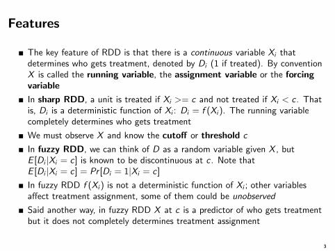
The key feature of RDD is that there is a continuous variable Xi thatdetermines who gets treatment, denoted by Di (1 if treated). By conventionX is called the running variable, the assignment variable or the forcingvariable

In sharp RDD, a unit is treated if Xi >= c and not treated if Xi < c . Thatis, Di is a deterministic function of Xi : Di = f (Xi ). The running variablecompletely determines who gets treatment

We must observe X and know the cutoff or threshold c

In fuzzy RDD, we can think of D as a random variable given X , butE [Di |Xi = c] is known to be discontinuous at c . Note thatE [Di |Xi = c] = Pr [Di = 1|Xi = c]

In fuzzy RDD f (Xi ) is not a deterministic function of Xi ; other variablesaffect treatment assignment, some of them could be unobserved

Said another way, in fuzzy RDD X at c is a predictor of who gets treatmentbut it does not completely determines treatment assignment

3

Identification

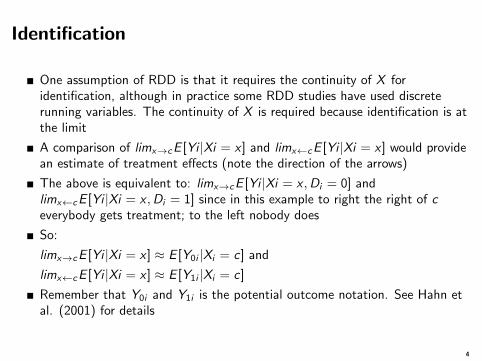
One assumption of RDD is that it requires the continuity of X foridentification, although in practice some RDD studies have used discreterunning variables. The continuity of X is required because identification is atthe limit

A comparison of limx→cE [Yi |Xi = x ] and limx←cE [Yi |Xi = x ] would providean estimate of treatment effects (note the direction of the arrows)

The above is equivalent to: limx→cE [Yi |Xi = x ,Di = 0] andlimx←cE [Yi |Xi = x ,Di = 1] since in this example to right the right of ceverybody gets treatment; to the left nobody does

So:

limx→cE [Yi |Xi = x ] ≈ E [Y0i |Xi = c] and

limx←cE [Yi |Xi = x ] ≈ E [Y1i |Xi = c]

Remember that Y0i and Y1i is the potential outcome notation. See Hahn etal. (2001) for details

4

Assumptions

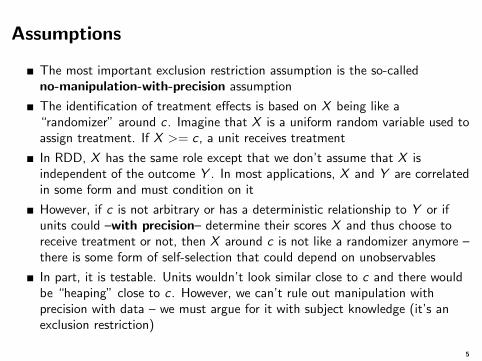
The most important exclusion restriction assumption is the so-calledno-manipulation-with-precision assumption

The identification of treatment effects is based on X being like a“randomizer” around c . Imagine that X is a uniform random variable used toassign treatment. If X >= c , a unit receives treatment

In RDD, X has the same role except that we don’t assume that X isindependent of the outcome Y . In most applications, X and Y are correlatedin some form and must condition on it

However, if c is not arbitrary or has a deterministic relationship to Y or ifunits could –with precision– determine their scores X and thus choose toreceive treatment or not, then X around c is not like a randomizer anymore –there is some form of self-selection that could depend on unobservables

In part, it is testable. Units wouldn’t look similar close to c and there wouldbe “heaping” close to c . However, we can’t rule out manipulation withprecision with data – we must argue for it with subject knowledge (it’s anexclusion restriction)

5

Estimation

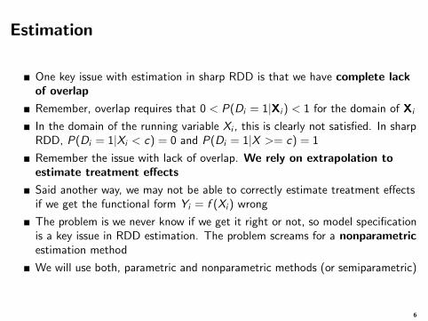
One key issue with estimation in sharp RDD is that we have complete lackof overlap

Remember, overlap requires that 0 < P(Di = 1|Xi ) < 1 for the domain of Xi

In the domain of the running variable Xi , this is clearly not satisfied. In sharpRDD, P(Di = 1|Xi < c) = 0 and P(Di = 1|X >= c) = 1

Remember the issue with lack of overlap. We rely on extrapolation toestimate treatment effects

Said another way, we may not be able to correctly estimate treatment effectsif we get the functional form Yi = f (Xi ) wrong

The problem is we never know if we get it right or not, so model specificationis a key issue in RDD estimation. The problem screams for a nonparametricestimation method

We will use both, parametric and nonparametric methods (or semiparametric)

6

Estimation

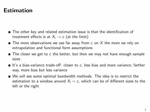
The other key and related estimation issue is that the identification oftreatment effects is at Xi → c (at the limit)

The more observations we use far away from c on X the more we rely onextrapolation and functional form assumptions

The closer we get to c the better, but then we may not have enough samplesizes

It’s a bias-variance trade-off: closer to c , less bias and more variance; fartherway, more bias but less variance

We will see some optimal bandwidth methods. The idea is to restrict theestimation to a window around Xi = c , which can be of different sizes to theleft or the right

7

Interpretation

In RDD, treatment effects are local average treatment effects or LATE

We don’t estimate the effect of getting the treatment, but rather the effectof getting the treatment for units that were close to c , not everybody in thesample (that’s the “local” part)

In a sense, this is the price we pay for being able to estimate treatmenteffects. However, in some applications, we might actually be interested inthis particular group and not others

In fuzzy RDD, we need to talk about the “complier” or the “marginalpatient” or “marginal unit”

8

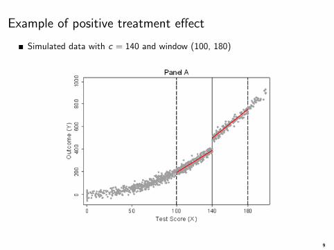
Example of positive treatment effect

Simulated data with c = 140 and window (100, 180)

9

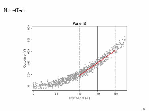
No effect

10

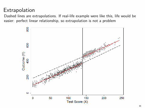
ExtrapolationDashed lines are extrapolations. If real-life example were like this, life would beeasier: perfect linear relationship, so extrapolation is not a problem

11

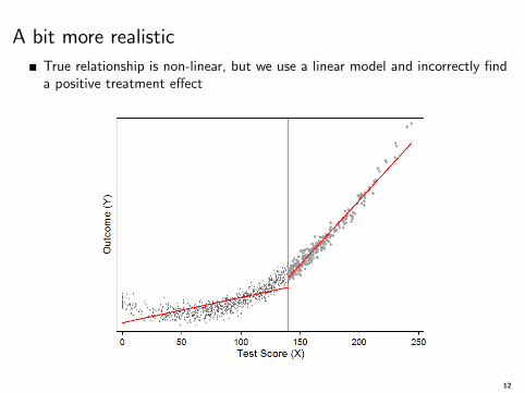
A bit more realistic

True relationship is non-linear, but we use a linear model and incorrectly finda positive treatment effect

12


Linear relationship between Y and X : Yi = β0 + β1Di + β3Xi + εi

Di = 1 if subject i received treatment and Di = 0 otherwise. We can alsowrite this as Di = 1(Xi ≥ c) or Di = 1[Xi≥c]

We can center center the running variable at c :

Yi = β0 + β1Di + β3(Xi − c) + εi

We have:

E [Yi |Di = 1,Xi = c] = β0 + β1 and E [Yi |Di = 0,Xi = c] = β0, so:

E [Yi |Di = 1,X = c]− E [Yi |Di = 0,Xi = c] = β1

Note that in Yi = β0 + β1Di + β3Xi + εi there is no interaction between Xand D so the effect of D does not depend to the value of X . In the abovemodels, β1 is the same

13


If we add an interaction, we have:

Yi = α0 + α1Di + α2(Xi − c) + α3(Xi − c)× Di + ηi

Now α1 is the treatment effect at Xi = c since at Xi = c , Xi − c = 0. Ifα3 6= 0, then the treatment effect at some other point could be different, butwe care about the treatment effect at the discontinuity

As we saw with some examples, the assumption of a linear relationshipbetween Y and X is strong and limiting. We could relax it

To keep the notation simpler, let X ≡ (X − c). The model then becomes:Yi = α0 + α1Di + α2Xi + α3Xi × Di + ηi

We could add a quadratic term to relax the linear assumption:Yi = α0 + α1Di + α2Xi + α3X

2i + α4Xi × Di + α5X

2i × Di + ηi

We could add polynomials of higher order. That used to be the usualrecommendation

14


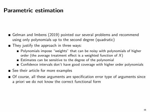
Gelman and Imbens (2019) pointed our several problems and recommendusing only polynomials up to the second degree (quadratic)

They justify the approach in three ways:

Polynomials impose “weights” that can be noisy with polynomials of higherorder (the average treatment effect is a weighted function of X )Estimates can be sensitive to the degree of the polynomialConfidence intervals don’t have good coverage with higher order polynomials

See their article for more examples

Of course, all these arguments are specification error type of arguments sincea priori we do not know the correct functional form

15

Covariates

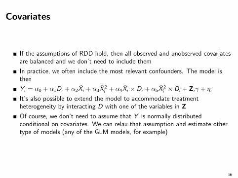
If the assumptions of RDD hold, then all observed and unobserved covariatesare balanced and we don’t need to include them

In practice, we often include the most relevant confounders. The model isthen

Yi = α0 + α1Di + α2Xi + α3X2i + α4Xi × Di + α5X

2i × Di + Ziγ + ηi

It’s also possible to extend the model to accommodate treatmentheterogeneity by interacting D with one of the variables in Z

Of course, we don’t need to assume that Y is normally distributedconditional on covariates. We can relax that assumption and estimate othertype of models (any of the GLM models, for example)

16

Testing assumptions

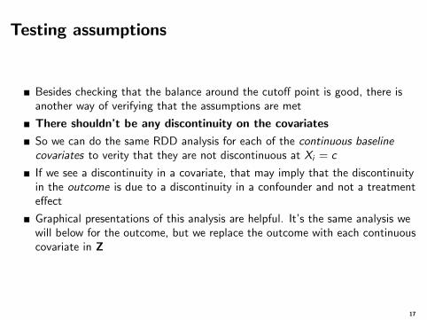
Besides checking that the balance around the cutoff point is good, there isanother way of verifying that the assumptions are met

There shouldn’t be any discontinuity on the covariates

So we can do the same RDD analysis for each of the continuous baselinecovariates to verity that they are not discontinuous at Xi = c

If we see a discontinuity in a covariate, that may imply that the discontinuityin the outcome is due to a discontinuity in a confounder and not a treatmenteffect

Graphical presentations of this analysis are helpful. It’s the same analysis wewill below for the outcome, but we replace the outcome with each continuouscovariate in Z

17

Data

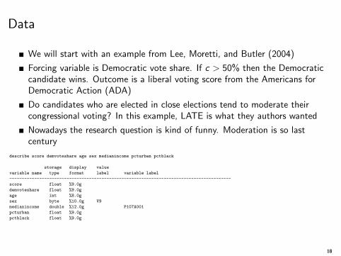
We will start with an example from Lee, Moretti, and Butler (2004)

Forcing variable is Democratic vote share. If c > 50% then the Democraticcandidate wins. Outcome is a liberal voting score from the Americans forDemocratic Action (ADA)

Do candidates who are elected in close elections tend to moderate theircongressional voting? In this example, LATE is what they authors wanted

Nowadays the research question is kind of funny. Moderation is so lastcentury

describe score demvoteshare age sex medianincome pcturban pctblack

storage display value

variable name type format label variable label

-----------------------------------------------------------------------------------------

score float %9.0g

demvoteshare float %9.0g

age int %8.0g

sex byte %10.0g V9

medianincome double %12.0g P107A001

pcturban float %9.0g

pctblack float %9.0g

18

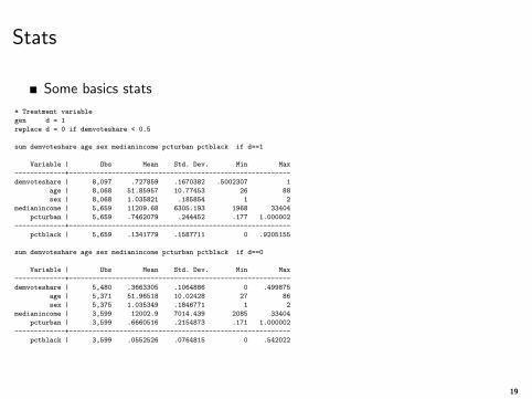
Stats

Some basics stats

* Treatment variable

gen d = 1

replace d = 0 if demvoteshare < 0.5

sum demvoteshare age sex medianincome pcturban pctblack if d==1

Variable | Obs Mean Std. Dev. Min Max

-------------+---------------------------------------------------------

demvoteshare | 8,097 .727859 .1670382 .5002307 1

age | 8,068 51.85957 10.77453 26 88

sex | 8,068 1.035821 .185854 1 2

medianincome | 5,659 11209.68 6305.193 1968 33404

pcturban | 5,659 .7462079 .244452 .177 1.000002

-------------+---------------------------------------------------------

pctblack | 5,659 .1341779 .1587711 0 .9205155

sum demvoteshare age sex medianincome pcturban pctblack if d==0


-------------+---------------------------------------------------------

demvoteshare | 5,480 .3663305 .1064886 0 .499875

age | 5,371 51.96518 10.02428 27 86

sex | 5,375 1.035349 .1846771 1 2

medianincome | 3,599 12002.9 7014.439 2085 33404

pcturban | 3,599 .6660516 .2154873 .171 1.000002

-------------+---------------------------------------------------------

pctblack | 3,599 .0552526 .0764815 0 .542022

19

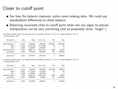
Closer to cutoff point

See how the balance improves; notice some missing data. We could usestandardized differences to check balance

Balancing covariates close to cutoff point when one can argue no precisemanipulation can be very convincing (not as propensity score “magic”)

sum demvoteshare age sex medianincome pcturban pctblack if d==1 & (demvoteshare>.40 & d

> emvoteshare<.60)


-------------+---------------------------------------------------------

demvoteshare | 2,204 .5484703 .0288765 .5002307 .5997699

age | 2,188 48.64762 10.40249 26 87

sex | 2,188 1.031993 .1760208 1 2

medianincome | 1,460 10691.14 5931.001 2608 30726

pcturban | 1,460 .7109719 .2302929 .193 1.000002

-------------+---------------------------------------------------------

pctblack | 1,460 .0751407 .0914119 0 .889344

sum demvoteshare age sex medianincome pcturban pctblack if d==0 & (demvoteshare>.40 & d

> emvoteshare<.60)


-------------+---------------------------------------------------------

demvoteshare | 2,428 .4502578 .0283787 .4000038 .499875

age | 2,354 51.34749 10.4509 27 83

sex | 2,358 1.025869 .1587792 1 2

medianincome | 1,303 10335.45 5845.274 2085 29850

pcturban | 1,303 .6469805 .212883 .171 1.000002

-------------+---------------------------------------------------------

pctblack | 1,303 .0633695 .0849373 0 .542022

20

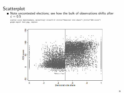
ScatterplotNote uncontested elections; see how the bulk of observations shifts afterc = 0.5scatter score demvoteshare, msize(tiny) xline(0.5) xtitle("Democrat vote share") ytitle("ADA score")

graph export lee1.png, replace

21

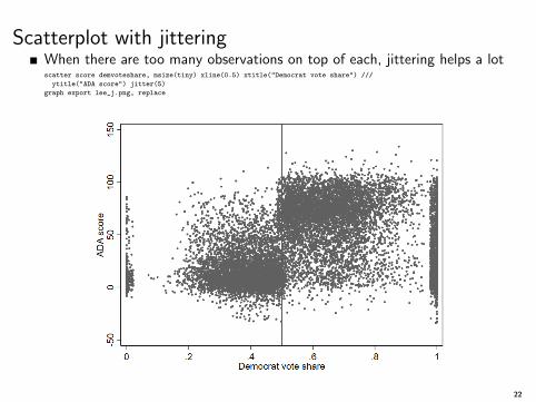
Scatterplot with jitteringWhen there are too many observations on top of each, jittering helps a lotscatter score demvoteshare, msize(tiny) xline(0.5) xtitle("Democrat vote share") ///

ytitle("ADA score") jitter(5)

graph export lee_j.png, replace

22

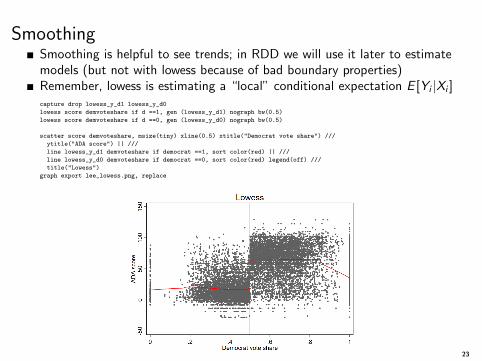
SmoothingSmoothing is helpful to see trends; in RDD we will use it later to estimatemodels (but not with lowess because of bad boundary properties)Remember, lowess is estimating a “local” conditional expectation E [Yi |Xi ]capture drop lowess_y_d1 lowess_y_d0

lowess score demvoteshare if d ==1, gen (lowess_y_d1) nograph bw(0.5)

lowess score demvoteshare if d ==0, gen (lowess_y_d0) nograph bw(0.5)

scatter score demvoteshare, msize(tiny) xline(0.5) xtitle("Democrat vote share") ///

ytitle("ADA score") || ///

line lowess_y_d1 demvoteshare if democrat ==1, sort color(red) || ///

line lowess_y_d0 demvoteshare if democrat ==0, sort color(red) legend(off) ///

title("Lowess")

graph export lee_lowess.png, replace

23

Things to note

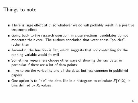
There is large effect at c , so whatever we do will probably result in a positivetreatment effect

Going back to the research question, in close elections, candidates do notmoderate their vote. The authors concluded that voter chose “policies”rather than

Around c , the function is flat, which suggests that not controlling for therunning variable would fit well

Sometimes researchers choose other ways of showing the raw data, inparticular if there are a lot of data points

I like to see the variability and all the data, but less common in publishedpapers

One option is to “bin” the data like in a histogram to calculate E [Yi |Xi ] inbins defined by Xi values

24

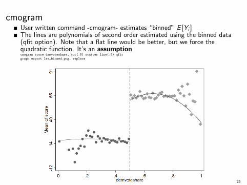
cmogramUser written command -cmogram- estimates “binned” E [Yi ]The lines are polynomials of second order estimated using the binned data(qfit option). Note that a flat line would be better, but we force thequadratic function. It’s an assumptioncmogram score demvoteshare, cut(.5) scatter line(.5) qfit

graph export lee_binned.png, replace

25

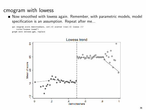
cmogram with lowessNow smoothed with lowess again. Remember, with parametric models, modelspecification is an assumption. Repeat after me...qui cmogram score demvoteshare, cut(.5) scatter line(.5) lowess ///

title("Lowess trend")

graph save cmlowes.gph, replace

26

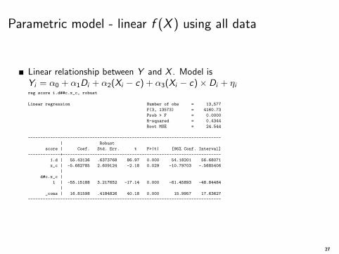
Parametric model - linear f (X ) using all data

Linear relationship between Y and X . Model isYi = α0 + α1Di + α2(Xi − c) + α3(Xi − c)× Di + ηireg score i.d##c.x_c, robust

Linear regression Number of obs = 13,577

F(3, 13573) = 4160.73

Prob > F = 0.0000

R-squared = 0.4344

Root MSE = 24.544

------------------------------------------------------------------------------

| Robust

score | Coef. Std. Err. t P>|t| [95% Conf. Interval]

-------------+----------------------------------------------------------------

1.d | 55.43136 .6373768 86.97 0.000 54.18201 56.68071

x_c | -5.682785 2.609124 -2.18 0.029 -10.79703 -.5685406

|

d#c.x_c |

1 | -55.15188 3.217652 -17.14 0.000 -61.45893 -48.84484

|

_cons | 16.81598 .4184826 40.18 0.000 15.9957 17.63627

------------------------------------------------------------------------------

27

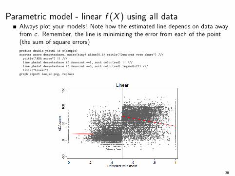
Parametric model - linear f (X ) using all dataAlways plot your models! Note how the estimated line depends on data awayfrom c . Remember, the line is minimizing the error from each of the point(the sum of square errors)predict double yhatm1 if e(sample)



line yhatm1 demvoteshare if democrat ==1, sort color(red) || ///

line yhatm1 demvoteshare if democrat ==0, sort color(red) legend(off) ///

title("Linear")

graph export lee_xc.png, replace

28

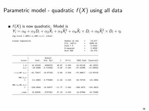
Parametric model - quadratic f (X ) using all data

f (X ) is now quadratic. Model isYi = α0 + α1Di + α2Xi + α3X

2i + α4Xi × Di + α5X

2i × Di + ηi

reg score i.d##(c.x_c##c.x_c), robust


F(5, 13571) = 2589.02

Prob > F = 0.0000

R-squared = 0.4559

Root MSE = 24.075

-------------------------------------------------------------------------------

| Robust


--------------+----------------------------------------------------------------

1.d | 44.40229 .9086222 48.87 0.000 42.62126 46.18331

x_c | -23.8496 6.710943 -3.55 0.000 -37.00398 -10.69522

|

c.x_c#c.x_c | -41.72917 14.67192 -2.84 0.004 -70.48817 -12.97018

|

d#c.x_c |

1 | 111.8963 9.779383 11.44 0.000 92.72733 131.0652

|

d#c.x_c#c.x_c |

1 | -229.9544 19.53577 -11.77 0.000 -268.2472 -191.6615

|

_cons | 15.60635 .5747061 27.16 0.000 14.47984 16.73285

-------------------------------------------------------------------------------

29

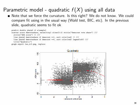
Parametric model - quadratic f (X ) using all dataNote that we force the curvature. Is this right? We do not know. We couldcompare fit using in the usual way (Wald test, BIC, etc). In the previousslide, quadratic seems to fit okpredict double yhatm2 if e(sample)



line yhatm2 demvoteshare if democrat ==1, sort color(red) || ///

line yhatm2 demvoteshare if democrat ==0, sort color(red) legend(off) ///

title("Quadratic")

graph export lee_xc2.png, replace

30

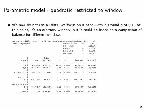
Parametric model - quadratic restricted to window

We now do not use all data; we focus on a bandwidth h around c of 0.1. Atthis point, it’s an arbitrary window, but it could be based on a comparison ofbalance for different windows

reg score i.d##(c.x_c##c.x_c) if (demvoteshare>.40 & demvoteshare<.60), robust


F(5, 4626) = 1132.17

Prob > F = 0.0000

R-squared = 0.5549

Root MSE = 21.327

-------------------------------------------------------------------------------

| Robust


--------------+----------------------------------------------------------------

1.d | 45.9283 1.851157 24.81 0.000 42.29915 49.55745

x_c | 38.63987 54.10772 0.71 0.475 -67.43706 144.7168

|

c.x_c#c.x_c | 295.1722 513.8466 0.57 0.566 -712.2123 1302.557

|

d#c.x_c |

1 | 6.507425 88.6282 0.07 0.941 -167.2461 180.261

|

d#c.x_c#c.x_c |

1 | -744.0247 867.1782 -0.86 0.391 -2444.108 956.0581

|

_cons | 17.71198 1.183657 14.96 0.000 15.39145 20.03251

-------------------------------------------------------------------------------

31

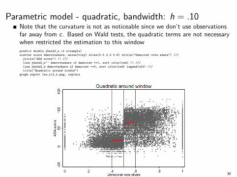
Parametric model - quadratic, bandwidth: h = .10Note that the curvature is not as noticeable since we don’t use observationsfar away from c . Based on Wald tests, the quadratic terms are not necessarywhen restricted the estimation to this windowpredict double yhatm2_w if e(sample)

scatter score demvoteshare, msize(tiny) xline(0.5 0.4 0.6) xtitle("Democrat vote share") ///


line yhatm2_w‘’ demvoteshare if democrat ==1, sort color(red) || ///

line yhatm2_w demvoteshare if democrat ==0, sort color(red) legend(off) ///

title("Quadratic around window")

graph export lee_xc2_w.png, replace

32

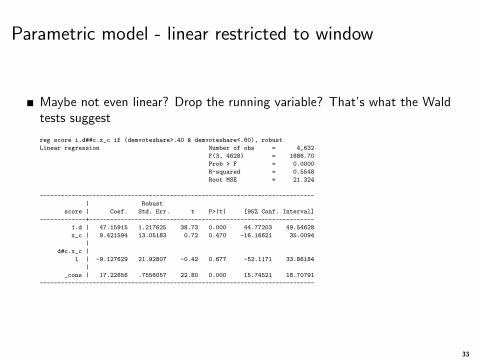
Parametric model - linear restricted to window

Maybe not even linear? Drop the running variable? That’s what the Waldtests suggest

reg score i.d##c.x_c if (demvoteshare>.40 & demvoteshare<.60), robust


F(3, 4628) = 1886.70

Prob > F = 0.0000

R-squared = 0.5548

Root MSE = 21.324

------------------------------------------------------------------------------

| Robust


-------------+----------------------------------------------------------------

1.d | 47.15915 1.217625 38.73 0.000 44.77203 49.54628

x_c | 9.421594 13.05183 0.72 0.470 -16.16621 35.0094

|

d#c.x_c |

1 | -9.127629 21.92807 -0.42 0.677 -52.1171 33.86184

|

_cons | 17.22656 .7556057 22.80 0.000 15.74521 18.70791

------------------------------------------------------------------------------

33

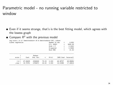
Parametric model - no running variable restricted towindow

Even if it seems strange, that’s is the best fitting model, which agrees withthe lowess graph

Compare R2 with the previous modelreg score i.d if (demvoteshare>.40 & demvoteshare<.60), robust


F(1, 4630) = 5630.09

Prob > F = 0.0000

R-squared = 0.5548

Root MSE = 21.32

------------------------------------------------------------------------------

| Robust


-------------+----------------------------------------------------------------

1.d | 47.64205 .6349402 75.03 0.000 46.39727 48.88684

_cons | 16.75791 .3765671 44.50 0.000 16.01966 17.49616

------------------------------------------------------------------------------

34

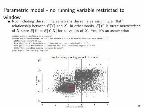
Parametric model - no running variable restricted towindow

Not including the running variable is the same as assuming a “flat”relationship between E [Y ] and X . In other words, E [Y ] is mean independentof X since E [Y ] = E [Y |X ] for all values of X . Yes, it’s an assumptionpredict double yhatflat_w if e(sample)

scatter score demvoteshare, msize(tiny) xline(0.5 0.4 0.6) xtitle("Democrat vote share") ///


line yhatflat_w‘’ demvoteshare if democrat ==1, sort color(red) || ///

line yhatflat_w demvoteshare if democrat ==0, sort color(red) legend(off) ///

title("Not including running variable in model")

graph export lee_flat.png, replace

35

Big picture

Any parametric model makes an assumption about the functional formbetween X and Y

If we thought that other covariates Zi should be added to the model, wecould repeat this same exercise but then graphs would need to be adjusted

Our final parametric model ended up being the simplest one

The best model depends on whether we use all the observations or not

The window is of course a very important consideration. We want tomake sure that observed covariates are well balanced

We should try other windows in sensitivity analyses, but we will see “optimal”windows as well

You can imagine that with less robust results you can find different resultsdepending on models

36

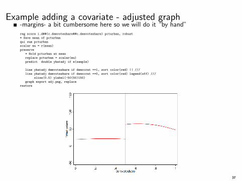
Example adding a covariate - adjusted graph-margins- a bit cumbersome here so we will do it “by hand”reg score i.d##(c.demvoteshare##c.demvoteshare) pcturban, robust

* Save mean of pcturban

qui sum pcturban

scalar mu = r(mean)

preserve

* Hold pcturban at mean

replace pcturban = scalar(mu)

predict double yhatadj if e(sample)

line yhatadj demvoteshare if democrat ==1, sort color(red) || ///

line yhatadj demvoteshare if democrat ==0, sort color(red) legend(off) ///

xline(0.5) ylabel(-50(50)150)

graph export adj.png, replace

restore

37

Nonparametric

Going back to the beginning. The issue with RDD estimation is that we needto get f (Xi ) right, but every single parametric model we try makes anassumption about the shape of f (Xi )

So rather than making assumptions about f (Xi ) we could estimate models inwhich we don’t assume a specific functional form – the data drives the shape,which is what lowess showed us

Lowess has poor boundary properties. RDD estimation is at X → c , and c isa boundary. We saw this in the first homework (or second?)

We will use instead Kernel-weighted local polynomial smoothing (command-lpoly-) since it’s easier to understand, but it has many limitation as it is

We will then move to what has now become the standard implementation forRDD using the user-written -rdrobust- command, which estimates similarnonparametric models

38

Kernel-weighted local polynomial smoothing, lpoly

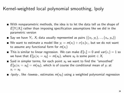
With nonparametric methods, the idea is to let the data tell us the shape ofE [Yi |Xi ] rather than imposing specification assumptions like we did in theparametric version

Say we have Yi , Xi data usually represented as pairs {(x1, y1), ..., (xn, yn)}We want to estimate a model like yi = m(xi ) + σ(xi )εi , but we do not wantto assume any functional form for m(xi )

This is similar to linear regression. We can make E [εi ] = 0 and var(εi ) = 1 sowe have that E [yi |xi = x0] = m(x0), where x0 is some point ∈ Xi

Said in simpler terms, for each point x0 we want to find the “smoothed”E [yi |xi = x0] = m(x0), which is of course the conditional mean of yi atxi = x0

-lpoly-, like -lowess-, estimates m(x0) using a weighted polynomial regression

39


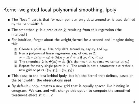
The “local” part is that for each point x0 only data around x0 is used definedby the bandwidth h

The smoothed yi is a prediction yi resulting from this regression (theintercept)

For intuition, forget about the weight/kernel for a second and imagine doingthis:

1 Choose a point x0. Use only data around x0, say xlb and xub2 Run a polynomial linear regression, say, of degree 2:

yi = β0 + β1(xi − x0) + β2(xi − x0)2 + εi if xlb ≤ xi ≤ xub3 The smoothed yi is m(x0) = β0 (it’s the mean at x0 since we center at x0)4 Repeat for every single point in x . The result is not a parameter but rather a

new grid or pairs {(x1, y1), ...(xn, yn)}This close to the idea behind lpoly, but it’s the kernel that defines, based onthe bandwdith, the observations used

By default -lpoly- creates a new grid that is equally spaced like binning incmogram. We can, and will, change this option to compute the smoothedtreatment effect at xi = c

40


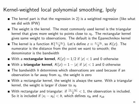
The kernel part is that the regression in 2) is a weighted regression (like whatwe did with IPW)

The weight is the kernel. The most commonly used kernel is the triangularkernel that gives more weight to points close to x0. The rectangular kernelgives same weight to observations. The default is the Epanechnikov kernel

The kernel is a function K ( xi−x0h ). Let’s define z ≡ xi−x0

h , so K (z). Thenumerator is the distance from the point we want to smooth; thedenominator is the bandwidth

With a rectangular kernel, K (z) = 1/2 if |z | < 1 and 0 otherwise

With a triangular kernel, K (z) = 1− |z | if |z | < 1 and 0 otherwise

The bandwidth h determines which observations are used because if anobservation is far away from x0, the weight is zero

With a rectangular kernel, the weight is always the same. With a triangularkernel, the weight is larger if closer to x0

With rectangular and triangular: if |xi−x0|h < 1, the observation is included.So it is included if |xi − x0| < h, which defines xlb and xub

41


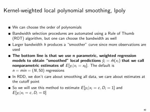
We can choose the order of polynomials

Bandwidth selection procedures are automated using a Rule of Thumb(ROT) algorithm, but one can choose the bandwidth as well

Larger bandwidth h produces a “smoother” curve since more observations areused

The bottom line is that we use n parametric, weighted regressionmodels to obtain “smoothed” local predictions yi = m(xi ) that we callnonparametric estimates of E [yi |xi = x0]. The default isn = min = (N, 50) regressions

In RDD, we don’t care about smoothing all data, we care about estimates atthe cutoff point

So we will use this method to estimate E [yi |xi = c ,Di = 1] andE [yi |xi = c ,Di = 0]

42

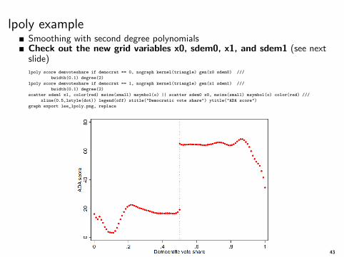
lpoly exampleSmoothing with second degree polynomialsCheck out the new grid variables x0, sdem0, x1, and sdem1 (see nextslide)lpoly score demvoteshare if democrat == 0, nograph kernel(triangle) gen(x0 sdem0) ///

bwidth(0.1) degree(2)

lpoly score demvoteshare if democrat == 1, nograph kernel(triangle) gen(x1 sdem1) ///

bwidth(0.1) degree(2)

scatter sdem1 x1, color(red) msize(small) msymbol(o) || scatter sdem0 x0, msize(small) msymbol(o) color(red) ///

xline(0.5,lstyle(dot)) legend(off) xtitle("Democratic vote share") ytitle("ADA score")

graph export lee_lpoly.png, replace

43

lpoly example

Remember, no parameter of interest is estimated even though we did used Nparametric regressions to get m(xi ) = yi

The original data is {(x1, y1), ..., (xn, yn)} and now we have a new grid{(x ′1, y1), ..., (x ′n, yn)}, where yi is the smoothed yi

We saved the new grid using the gen() option in variables x0, sdem0, x0, andsdem0Remember, by default, lpoly uses an equally spaced grid to divide the x axis,much like cmogram:. list x0 sdem0 x1 sdem1 in 1/5

+-----------------------------------------------+

| x0 sdem0 x1 sdem1 |

|-----------------------------------------------|

1. | 0 16.273488 .50023067 65.160334 |

2. | .01020153 13.828991 .51043004 64.363744 |

3. | .02040306 12.661728 .52062942 64.24728 |

4. | .03060459 14.445168 .53082879 64.335256 |

5. | .04080613 12.304093 .54102817 64.393172 |

+-----------------------------------------------+

44

lpoly example

We can obtain the treatment effect but saving the smoothed values at thecutoff point xi = c = 0.5

Again, by default lpoly builds an equally spaced grid to calculate E [yi |xi ]],but we can change that with the “at” option (we could, for example, ask-lpoly- to calculate E [yi |xi ] at each of the observed values)

We need to define a variable with cutoff point (the “at” option takes avariable)gen forat = 0.5 in 1

capture drop sdem0 sdem1

lpoly score demvoteshare if democrat == 0, nograph kernel(triangle) gen(sdem0) degree(2) ///

at(forat) bwidth(0.1)



gen dif = sdem1 - sdem0

list sdem1 sdem0 dif in 1/1

+----------------------------------+

| sdem1 sdem0 dif |

|----------------------------------|

1. | 65.190977 19.275926 45.91505 |

+----------------------------------+

So treatment effect at c is 45.91

Think about this for a second. We are using all the data, but the estimate atc here is local because of h. So in this sense, we are not using data far awayfrom c to estimate the treatment effect at xi = c

45

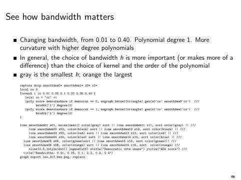
See how bandwidth matters

Changing bandwidth, from 0.01 to 0.40. Polynomial degree 1. Morecurvature with higher degree polynomials

In general, the choice of bandwidth h is more important (or makes more of adifference) than the choice of kernel and the order of the polynomial

gray is the smallest h; orange the largest

capture drop smoothdem0* smoothdem1* x0* x1*

local co 0

foreach i in 0.01 0.05 0.1 0.20 0.30 0.40 {

local co = ‘co’ +1

lpoly score demvoteshare if democrat == 0, nograph kernel(triangle) gen(x0‘co’ smoothdem0‘co’) ///

bwidth(‘i’) degree(2)

lpoly score demvoteshare if democrat == 1, nograph kernel(triangle) gen(x1‘co’ smoothdem1‘co’) ///

bwidth(‘i’) degree(2)

}

line smoothdem01 x01, msize(small) color(gray) sort || line smoothdem11 x11, sort color(gray) || ///

line smoothdem02 x02, color(black) sort || line smoothdem12 x12, sort color(black) || ///

line smoothdem03 x03, color(red) sort || line smoothdem13 x13, sort color(red) || ///

line smoothdem04 x04, color(blue) sort || line smoothdem14 x14, sort color(blue) || ///

line smoothdem05 x05, color(green)sort || line smoothdem15 x15, sort color(green)|| ///

line smoothdem06 x06, color(orange) sort || line smoothdem16 x16, sort color(orange) ///

xline(0.5,lstyle(dot)) legend(off) xtitle("Democratic vote share") ytitle("ADA score") ///

title("Bandwidths: 0.01, 0.05, 0.1, 0.2, 0.3, 0.4")

graph export lee_dif_bws.png, replace

46

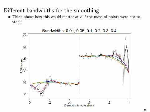
Different bandwidths for the smoothingThink about how this would matter at c if the mass of points were not sostable

47

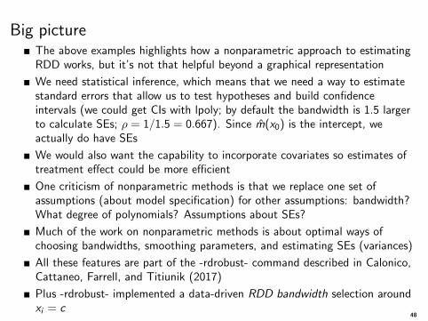
Big pictureThe above examples highlights how a nonparametric approach to estimatingRDD works, but it’s not that helpful beyond a graphical representation

We need statistical inference, which means that we need a way to estimatestandard errors that allow us to test hypotheses and build confidenceintervals (we could get CIs with lpoly; by default the bandwidth is 1.5 largerto calculate SEs; ρ = 1/1.5 = 0.667). Since m(x0) is the intercept, weactually do have SEs

We would also want the capability to incorporate covariates so estimates oftreatment effect could be more efficient

One criticism of nonparametric methods is that we replace one set ofassumptions (about model specification) for other assumptions: bandwidth?What degree of polynomials? Assumptions about SEs?

Much of the work on nonparametric methods is about optimal ways ofchoosing bandwidths, smoothing parameters, and estimating SEs (variances)

All these features are part of the -rdrobust- command described in Calonico,Cattaneo, Farrell, and Titiunik (2017)

Plus -rdrobust- implemented a data-driven RDD bandwidth selection aroundxi = c

48

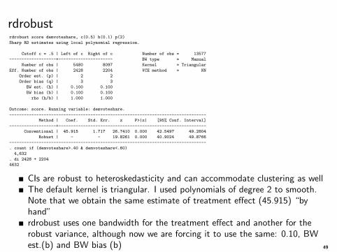
rdrobustrdrobust score demvoteshare, c(0.5) h(0.1) p(2)

Sharp RD estimates using local polynomial regression.

Cutoff c = .5 | Left of c Right of c Number of obs = 13577

-------------------+---------------------- BW type = Manual

Number of obs | 5480 8097 Kernel = Triangular

Eff. Number of obs | 2428 2204 VCE method = NN

Order est. (p) | 2 2

Order bias (q) | 3 3

BW est. (h) | 0.100 0.100

BW bias (b) | 0.100 0.100

rho (h/b) | 1.000 1.000

Outcome: score. Running variable: demvoteshare.

--------------------------------------------------------------------------------

Method | Coef. Std. Err. z P>|z| [95% Conf. Interval]

-------------------+------------------------------------------------------------

Conventional | 45.915 1.717 26.7410 0.000 42.5497 49.2804

Robust | - - 19.8261 0.000 40.9024 49.8766

--------------------------------------------------------------------------------

. count if (demvoteshare>.40 & demvoteshare<.60)

4,632

. di 2428 + 2204

4632

CIs are robust to heteroskedasticity and can accommodate clustering as wellThe default kernel is triangular. I used polynomials of degree 2 to smooth.Note that we obtain the same estimate of treatment effect (45.915) “byhand”rdrobust uses one bandwidth for the treatment effect and another for therobust variance, although now we are forcing it to use the same: 0.10, BWest.(b) and BW bias (b) 49

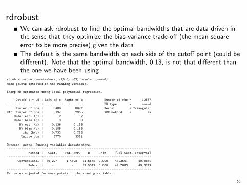
rdrobustWe can ask rdrobust to find the optimal bandwidths that are data driven inthe sense that they optimize the bias-variance trade-off (the mean squareerror to be more precise) given the data

The default is the same bandwidth on each side of the cutoff point (could bedifferent). Note that the optimal bandwidth, 0.13, is not that different thanthe one we have been using

rdrobust score demvoteshare, c(0.5) p(2) bwselect(mserd)

Mass points detected in the running variable.



-------------------+---------------------- BW type = mserd





BW est. (h) | 0.136 0.136

BW bias (b) | 0.185 0.185

rho (h/b) | 0.732 0.732

Unique obs | 2770 3351


--------------------------------------------------------------------------------


-------------------+------------------------------------------------------------

Conventional | 46.227 1.4598 31.6675 0.000 43.3661 49.0882

Robust | - - 27.5319 0.000 42.7683 49.3242

--------------------------------------------------------------------------------

Estimates adjusted for mass points in the running variable.

50

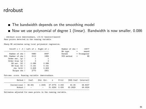
rdrobust

The bandwidth depends on the smoothing model

Now we use polynomial of degree 1 (linear). Bandwidth is now smaller, 0.086

. rdrobust score demvoteshare, c(0.5) bwselect(mserd)




-------------------+---------------------- BW type = mserd





BW est. (h) | 0.086 0.086

BW bias (b) | 0.141 0.141

rho (h/b) | 0.609 0.609



--------------------------------------------------------------------------------


-------------------+------------------------------------------------------------

Conventional | 46.491 1.2405 37.4775 0.000 44.06 48.9227

Robust | - - 31.4254 0.000 43.2929 49.0524

--------------------------------------------------------------------------------


51

Plots

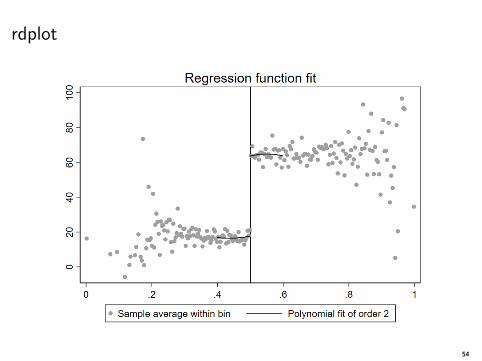
rdrobust implement plots using a combination of tools we saw before

It does create bins rather than plotting the raw data in the same way we didit with cmogram, but using a different algorithm

The plots match the nonparametric treatment effect estimates and thesmoothing model

As usual, we can customize the plot (see graph options()) but we will use thedefaults here

52

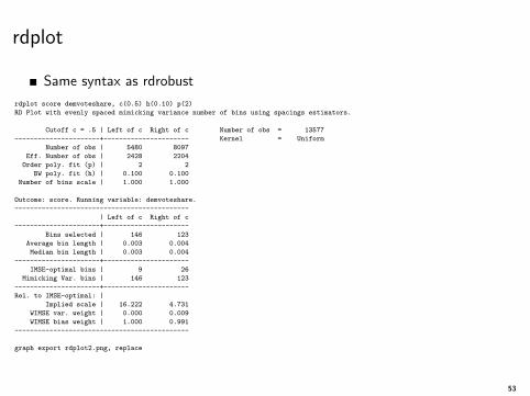
rdplot

Same syntax as rdrobust

rdplot score demvoteshare, c(0.5) h(0.10) p(2)

RD Plot with evenly spaced mimicking variance number of bins using spacings estimators.


----------------------+---------------------- Kernel = Uniform

Number of obs | 5480 8097

Eff. Number of obs | 2428 2204

Order poly. fit (p) | 2 2

BW poly. fit (h) | 0.100 0.100

Number of bins scale | 1.000 1.000


---------------------------------------------

| Left of c Right of c

----------------------+----------------------

Bins selected | 146 123

Average bin length | 0.003 0.004

Median bin length | 0.003 0.004

----------------------+----------------------

IMSE-optimal bins | 9 26

Mimicking Var. bins | 146 123

----------------------+----------------------

Rel. to IMSE-optimal: |

Implied scale | 16.222 4.731

WIMSE var. weight | 0.000 0.009

WIMSE bias weight | 1.000 0.991

---------------------------------------------

graph export rdplot2.png, replace

53

rdplot

54

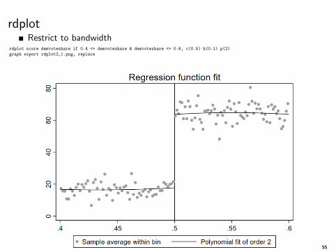
rdplotRestrict to bandwidth

rdplot score demvoteshare if 0.4 <= demvoteshare & demvoteshare <= 0.6, c(0.5) h(0.1) p(2)

graph export rdplot2_1.png, replace

55

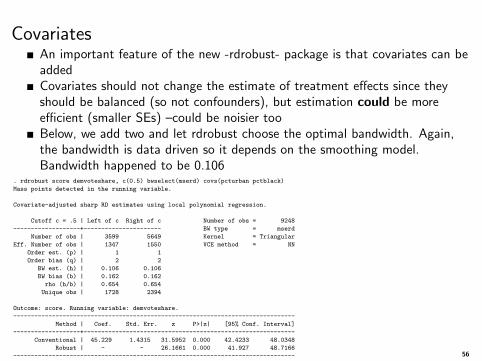
CovariatesAn important feature of the new -rdrobust- package is that covariates can beaddedCovariates should not change the estimate of treatment effects since theyshould be balanced (so not confounders), but estimation could be moreefficient (smaller SEs) –could be noisier tooBelow, we add two and let rdrobust choose the optimal bandwidth. Again,the bandwidth is data driven so it depends on the smoothing model.Bandwidth happened to be 0.106

. rdrobust score demvoteshare, c(0.5) bwselect(mserd) covs(pcturban pctblack)


Covariate-adjusted sharp RD estimates using local polynomial regression.


-------------------+---------------------- BW type = mserd





BW est. (h) | 0.106 0.106

BW bias (b) | 0.162 0.162

rho (h/b) | 0.654 0.654



--------------------------------------------------------------------------------


-------------------+------------------------------------------------------------

Conventional | 45.229 1.4315 31.5952 0.000 42.4233 48.0348

Robust | - - 26.1661 0.000 41.927 48.7166

--------------------------------------------------------------------------------

Covariate-adjusted estimates. Additional covariates included: 2


56

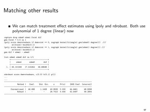
Matching other results

We can match treatment effect estimates using lpoly and rdrobust. Both usepolynomial of 1 degree (linear) now

capture drop sdem0 sdem1 forat dif

gen forat = 0.5 in 1







+----------------------------------+

| sdem1 sdem0 dif |

|----------------------------------|

1. | 64.101309 17.415352 46.68596 |

+----------------------------------+

rdrobust score demvoteshare, c(0.5) h(0.1) p(1)

...

...

--------------------------------------------------------------------------------


-------------------+------------------------------------------------------------

Conventional | 46.686 1.1428 40.8525 0.000 44.4461 48.9258

Robust | - - 26.7410 0.000 42.5497 49.2804

--------------------------------------------------------------------------------

57

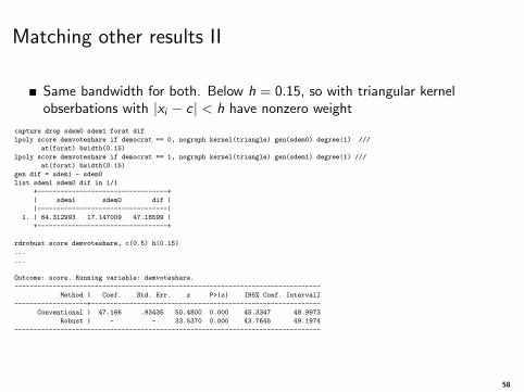
Matching other results II

Same bandwidth for both. Below h = 0.15, so with triangular kernelobserbations with |xi − c | < h have nonzero weight

capture drop sdem0 sdem1 forat dif







+----------------------------------+

| sdem1 sdem0 dif |

|----------------------------------|

1. | 64.312993 17.147009 47.16599 |

+----------------------------------+

rdrobust score demvoteshare, c(0.5) h(0.15)

...

...


--------------------------------------------------------------------------------


-------------------+------------------------------------------------------------

Conventional | 47.166 .93435 50.4800 0.000 45.3347 48.9973

Robust | - - 33.5370 0.000 43.7645 49.1974

--------------------------------------------------------------------------------

58

Important: rdrobust is really a parametric methodgiven a bandwidth

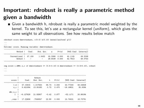
Given a bandwidth h, rdrobust is really a parametric model weighted by thekernel. To see this, let’s use a rectangular kernel (uniform), which gives thesame weight to all observations. See how results below match

rdrobust score demvoteshare, c(0.5) h(0.10) kernel(uniform) p(1)

...

...


--------------------------------------------------------------------------------


-------------------+------------------------------------------------------------

Conventional | 47.159 1.0432 45.2066 0.000 45.1145 49.2038

Robust | - - 28.6039 0.000 42.7813 49.0753

--------------------------------------------------------------------------------

reg score i.d##c.x_c if demvoteshare >= (0.5-0.10) & demvoteshare <= (0.5+0.10), robust

...

...

------------------------------------------------------------------------------

| Robust


-------------+----------------------------------------------------------------

1.d | 47.15915 1.217625 38.73 0.000 44.77203 49.54628

x_c | 9.421594 13.05183 0.72 0.470 -16.16621 35.0094

|

d#c.x_c |

1 | -9.127629 21.92807 -0.42 0.677 -52.1171 33.86184

|

_cons | 17.22656 .7556057 22.80 0.000 15.74521 18.70791

------------------------------------------------------------------------------

59

Important: rdrobust is really a parametric methodgiven a bandwidth

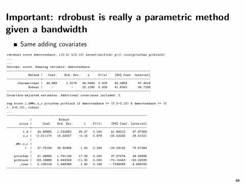
Same adding covariates

rdrobust score demvoteshare, c(0.5) h(0.10) kernel(uniform) p(1) covs(pcturban pctblack)

...

...


--------------------------------------------------------------------------------


-------------------+------------------------------------------------------------

Conventional | 44.869 1.3179 34.0464 0.000 42.2859 47.4518

Robust | - - 22.1095 0.000 41.6342 49.7338

--------------------------------------------------------------------------------

Covariate-adjusted estimates. Additional covariates included: 2

reg score i.d##c.x_c pcturban pctblack if demvoteshare >= (0.5-0.10) & demvoteshare <= (0

> .5+0.10), robust

...

------------------------------------------------------------------------------

| Robust


-------------+----------------------------------------------------------------

1.d | 44.86885 1.532883 29.27 0.000 41.86313 47.87456

x_c | -2.511174 16.33057 -0.15 0.878 -34.53255 29.51021

|

d#c.x_c |

1 | 27.79169 26.45986 1.05 0.294 -24.09145 79.67484

|

pcturban | 31.08685 1.791139 17.36 0.000 27.57474 34.59896

pctblack | -63.18889 5.592308 -11.30 0.000 -74.15443 -52.22335

_cons | 2.106124 1.448386 1.45 0.146 -.7339069 4.946155

------------------------------------------------------------------------------

60

Limitations, other things

Helpful to explore the sensitivity of estimates to model specification usingnonparametric methods

In this example, not much difference, but in other situations it could be aworld of difference between parametric and nonparametric, which couldmean model specification issues or just a lot of noise in the data

When there is more noise than signal, different models will produce differenceanswers, in magnitude, direction, and statistical significance

Nonparametric methods are not always better; they do have many underlyingassumptions. They are less efficient when the parametric model is right.Problem is only in simulations we know for sure what is the “right” model

No way to test for treatment heterogeniety with current nonparametricmodels. We could estimate stratified models, not as efficient as interactions

Summary is that we should try both and be concerned when resultsdiffer (and try to figure out why)

61

Fuzzy RDD, instrumental variables detour

If we randomize people into groups using a uniform random variable U, U isan unconditional randomizer. It works because U is uncorrelated in anyfunctional form with any observed and unobserved covariate and also theoutcome (it’s random)

In RDD the forcing variable X is like a conditional randomizer but onlyclose to cutoff point c and we must condition for X . It’s conditionalbecause it’s like the example of conditional randomization when we use thevalues of a variable –severity– to randomize people into treatments. The keydifference is that RDD induces a discontinuity – every single person is giventreatment if Xi ≥ c

The idea behind an instrumental variable approach is that the instrument Zacts like a psuedo “randomizer” in the sense that Z is a strong predictor oftreatment but it must be conditional independent of the outcome

The “conditional independent of the outcome” part is the exclusionrestriction, or the assumption that must be argued and in practice is sodifficult to determine with clarity

62

Encouragement design

Let’s go back to the example of an encouragement design. The idea is torandomly assign people into two groups and then encourage one group toreceive a treatment or intervention (say, to receive regular preventive services)

In this setting, randomization is about encouragement not actually receivingtreatment. If we compare an outcome Y in both groups, we would obtain anestimate of encouraging people to do something, not an estimate of receivingthe treatment. That is, intent-to-treat (ITT)

You can imagine that there are different types of people. No matter what youdo, some do not want to go to the doctor (never-takers), while other peopleare very concerned about their health and will get preventive servicesregardless of what you tell them (always-takers)

Then there is a group of people whose behavior can be changed. After theencouragement, they decide to follow the recommendation. These are thecompliers

Finally, there could be contrarians: they do the opposite of what they aretold. We must rule them out

63

Encouragement design

Randomization ensures that the distribution of the type of people isthe same in the treatment and control group

Other than ITT, the estimate of treatment effect we could obtain is on thecompliers, sometimes called the “complier average treatment effect” or theLATE

Keep in mind that in this setting nothing prevents people in the controlgroup to get preventive services. The always-takers will in fact get preventiveservices. The never-takers in the control group will not. But the compliersmay not because we have not encourage them to do so, although some coulddo it anyway

When we think about counterfactuals, the control group can only provide aconterfactual for the compliers: what would have happened if the treated hadnot been encouraged to be treated. That’s why we can only obtain LATE forthe compliers

In this example, the randomizer (instrument) was actually the randomtreatment assignment: it’s a strong predictor of receiving treatment and isuncorrelated with outcomes

64

EstimationOur target of estimation is not the effect of encouraging people to receivepreventive services but rather the effect of receiving preventive services on anoutcome Y , say a measure of health status

We will denote prevention services as P (say preventive doctor visits). Thecausal, population model we care about is

Yi = β0 + β1Pi + εiIn the above model, P and ε are correlated since we know that P is alsocorrelated with being randomized into the encouragement group, which wedenote with a dummy variable Zi . What we don’t observed are factors thatexplain who would follow the recommendation and go visit the doctor. Thisis the unobserved selection. If we add Z to the above model, its coefficientwould be 0 because of randomization (this becomes important later)

If we compare E [Yi |Zi = 1]− E [Yi |Zi = 0] we would be estimating theaverage difference in health status between the group that was encouraged toreceived treatment and the group that was not encouraged (ITT)

Intuitively, the piece that is missing is that in both groups people could havereceived preventive services, the actual treatment. So we could “weight” ITTby the (average) difference in preventive differences services received by eachgroup: E [Pi |Zi = 1]− E [Pi |Zi = 0]

65

Estimation and intuitionIt turns out that this is actually the estimator we want:

β1 = E [Yi |Zi=1]−E [Yi |Zi=0]E [Pi |Zi=1]−E [Pi |Zi=0]

The above estimator is called the Wald estimator (introduced in the contextof measurement error models; see AP page 127)

If in both groups prevention services received are the same, then thedenominator is zero and the treatment effect is infinity

With a small difference, β1 could get very large. In words, being randomizedinto the encouragement group is not a strong predictor of receiving treatment(this is what is called a weak instrument)

If more people in the control group actually received treatment, then thetreatment effect would flip signs

If being randomized into the encouragement group makes a difference inreceiving preventive services (strong predictor), the differenceE [Pi |Zi = 1]− E [Pi |Zi = 0] would be large. We “adjust” or weight thenumerator by more

Again, this new estimate only applies to the compliers, because theencouragement only worked on this “local” set of participants (hence, LATE)

66

Estimation, more generalIn a more general case without covariates and with a possibly continuousinstrument Z , we can think of a system of equations:

1 Pi = α0 + α1Zi + εi2 Yi = γ0 + γ1Pi + ηi

In the first equation, we estimate how the instrument Z predict thetreatment P

The second equation is the outcome equation, which we know we can’testimate as is because P is not random, there is selection (ignorability fails).We don’t know what factor explain why people decided to get preventiveservices; these factors are likely unobserved

What we do is exploit the fact that we know there is anexternal/exogenous/randomizer factor Z , which we called the instrument,that strongly predicts who gets prevention services and because it’s arandomizer we assume it is not related to the outcome. Another way peoplesay this is something like “we exploit the variability in P induced by Z”

The system of equations can be estimated using two-stage least squares(2SLS) or using structural model equations (SEM). In 2SLS, predictions frommodel 1) are used to estimate model 2: Yi = γ0 + γ1Pi + ηi

67

Assumptions

Again, with the more general setting:

1 Pi = α0 + α1Zi + εi2 Yi = γ0 + γ1Pi + ηi

One assumption is that the instrument Z must be uncorrelated with both εand η, which amounts to assuming ignorability of the instrument and theexclusion restriction that says that the only way the instrument affects theoutcome is through the treatment

We are safe when the instrument is randomization since randomization is notrelated to the outcome (treatment assignment is random)

It’s very hard to come up with instruments in the wild. In some cases,controlling for variables could give us conditional ignorability and make theexclusion restriction hold (or hold “better”), so we would add a vector ofvariables X in both regressions

68

Estimation IIHere is one way we could derive the instrument in the more general setting ofZ continuous, following Gelman, Hill, and Vehtari (2020). We can rewrite:

1 Pi = α0 + α1Zi + εi2 Yi = γ0 + γ1Pi + γ2Zi + ηi

Since we assume the exclusion restriction, γ2 = 0 in equation (2) (thinkabout it, this is important. It’s only zero if P is in the model). Our goal isto obtain γ1 accounting for selection on unobservables contained in η

Now plug in equation (1) into equation (2):

Yi = γ0 + γ1(α0 + α1Zi ) + γ2Zi + ηi = (γ0 + γ1α0) + (α1γ1 + γ2)Zi + ηi (3)

We could rewrite (3) as Yi = β1 + β2Zi + ei , which we could estimate usingthe data. Here, β2 = (α1γ1 + γ2), which means γ1 = β2−γ2

α1

Since we know γ2 = 0 due to the exclusion restriction, we are left withγ1 = β2

α1

And that’s the 2SLS estimate, similar to the Wald estimate with a binaryinstrument. Note that α1 is the coefficient of Z in (1). If close to zero, wehave a weak instrument. β2 is the ITT

Note how we get a different estimate, γbiased1 = β2

α1− γ2

α1, if the exclusion

restriction in fact doesn’t hold69

Back to fuzzy RDD

The connection with fuzzy RDD is straightforward

The assignment variable X at the cutoff point c (the instrument) must be astrong predictor of receiving treatment; that’s the first condition

If the RDD assumptions hold, around Xi = c , conditioning on the runningvariable Xi , the exclusion restriction holds too: the only way the instrumentaffects the outcome is through the treatment

In this sense, the assumptions of fuzzy RDD are milder than the assumptionsof IV (see Hahn et al., 2001)

Estimation follows IV in parametric approaches

-rdrobust- estimates nonparametric fuzzy RDD with the option fuzzy()

Remember that the key insight is that we are exploiting the fact that thediscontinuity in Xi = c is a strong predictor of treatment, which we mustassume is not related to the outcome Y (only through treatment). Absence atreatment, there would have been continuity

70

There is much more to it

More details next semester. The world of IV is vast...

For an application of IVs when the instrument is randomization, see Baickeret al. (2013) describing Medicaid’s Oregon experiment

71

Documents

Week 10: Regression discontinuity designs