Week 6 - Confounding 1 C onfounding Lydia B. Zablotska, MD, PhD Associate Professor Department of Epidemiology and Biostatistics

Week 6 - Confounding1

Confounding

Lydia B. Zablotska, MD, PhDAssociate ProfessorDepartment of Epidemiology and Biostatistics

Week 6 – Confounding2

Learning Objectives

Review and expand definition of confounding Methods to control confounding in the design of the study:

– Randomization– Restriction – Matching and analysis of matched data

Statistical adjustment of confounding effects– Stratification– Multivariate adjustment models– Under- and over-adjustment and estimation of amount

of confounding– Propensity scores – Structural measures and G-estimation

Residual and unmeasured confounding


Confounding

Importance of confounding in experimental research and observational studies

Estimation of effects in observational studies– Comparison of exposed and unexposed– Unexposed represent what the frequency of disease would

have been in the exposed cohort had exposure been absent (counterfactual)

– Exposed cohort may differ from the unexposed cohort on many factors besides exposure, i.e. the use of unexposed as a referent for the exposed is confounded

– “Mixing of effects” does not mean that exposure has to have an effect [Latin confundere – to mix together]

Hosmer and Lemeshow, 1989: http://epiville.ccnmtl.columbia.edu/interactive/confounding01.html

RG Ch 9


Criteria for confounding: Well-known?

1. Associated with disease

2. Associated with exposure

3. Not in the causal pathway from exposure to disease

RG Ch 9


Criteria for confounding: Some caveats

1. Associated with disease Predictive of disease occurrence apart from its association

with exposure (extraneous risk factor) Should involve a mechanism other than the one under

study Associated with disease among unexposed (referent

group) Does not have to actually cause the outcome, but must

affect it in some way, predict who will develop disease

RG Ch 9, 12



2. Associated with exposure Associated with exposure among the source population for

cases, i.e. in the control group of the case-control study Association between exposure and confounder among

cases is not a valid estimate of the association in the source population

RG Ch 9



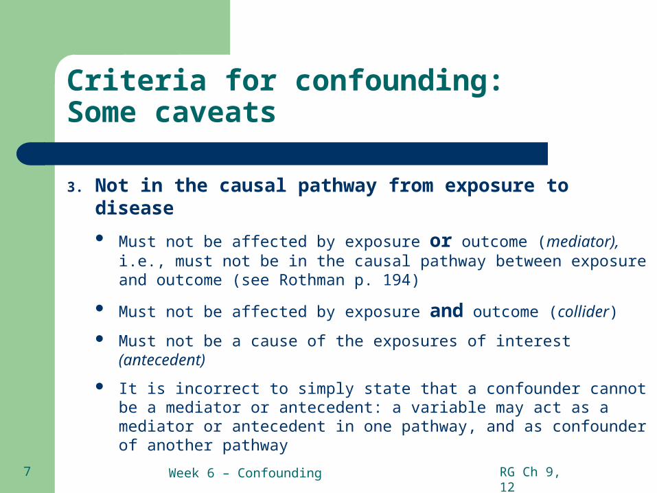
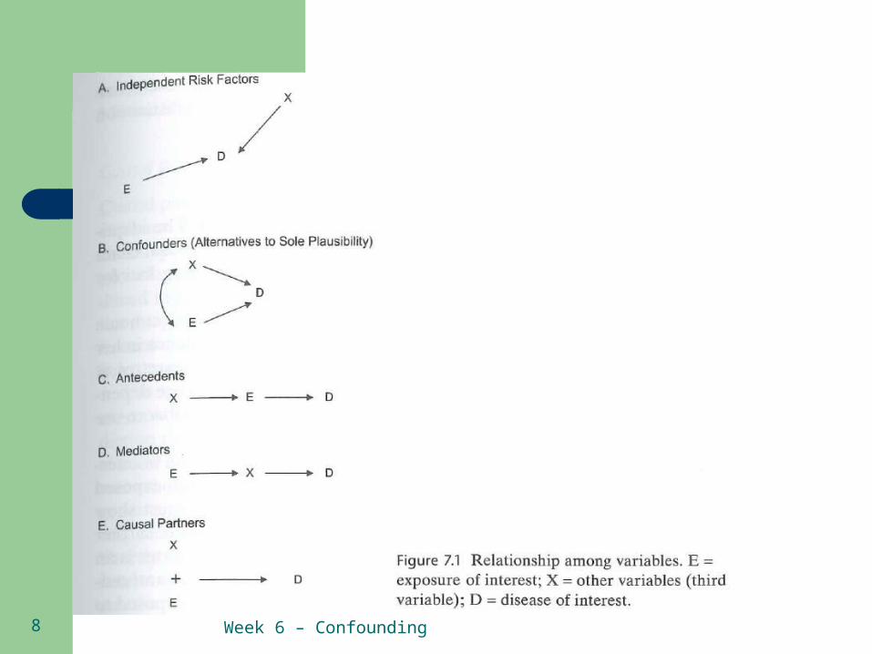
3. Not in the causal pathway from exposure to disease

Must not be affected by exposure or outcome (mediator), i.e., must not be in the causal pathway between exposure and outcome (see Rothman p. 194)

Must not be affected by exposure and outcome (collider)

Must not be a cause of the exposures of interest (antecedent)

It is incorrect to simply state that a confounder cannot be a mediator or antecedent: a variable may act as a mediator or antecedent in one pathway, and as confounder of another pathway

RG Ch 9, 12



Linguistic ability in young adulthood and Alzheimer’s disease



Confounding: Some caveats, continued

Even if all three criteria are satisfied, the potential confounding factor may not produce any spurious excess or deficit of disease among exposed:

– If there are multiple confounding variables whose effects are perfectly balanced

The degree of confounding is of much greater concern than its mere presence or absence

RG Ch 9


Adjustment for confounding effects of known and measured confounders: Magnitude of confounding

“Simpson’s Paradox” is rare– an extraneous factor, i.e. confounding factor, can change the

direction of association between primary exposure of interest and outcome

– In most studies a RR or OR of 2 or more is unlikely to be entirely explained by a single confounder

Example: association between prenatal exposure to the Dutch Hunger Winter and adult schizophrenia could be confounded by social class (from Psychiatric Epidemiology: Searching for the Causes of Mental Disorders (2006) by Ezra Susser et al.)



Dutch Hunger Winter and adult schizophrenia

SES as a confounder (C): C-E association: higher social class women were somewhat better nourished; over-

represented among exposed (ratio of upper SES to lower SES in exposed 3:2, in unexposed 1:1)

C-O association: most studies show that lower SES is associated with higher risk of schizophrenia, but one study in Holland showed that higher parental social class was a significant risk factor for schizophrenia in offspring (university town based study of 34 psychiatric hospitalizations)

Assuming higher SES is associated with schizophrenia: 5,000 E+ and 100,000 E- E-O not associated, i.e. risk in E+ and E- is the same C-O associated, i.e. risk in C+ (high SES) = 0.5%, C- (lower SES) = 0.25% Risk (O/ E+) = {(0.5%*3,000) + (0.25%*2,000)} /5,000 = 20 / 5,000 = 4 per 1,000 Risk (O/ E-)={(0.5%*50,000) + (0.25%*50,000)} /100,000 = 375 / 100,000 = 3.75 per

1,000 RR=4 / 3.75 = 1.07 Even when assuming that E has no effect and C has a strong effect on O, the artifactual

RR adjusted for C is barely detectable and cannot account for observed RR of 2.0.


Adjustment for confounding effects of known and measured confounders: Magnitude of confounding, continued

Confounding effects could be cumulative. Thus, several confounders with modest individual impact taken together, may account for an appreciable risk ratio distortion

Magnitude of confounding is a result of the strength of the associations between the confounder AND BOTH exposure and disease

Do tests of statistical significance to evaluate presence of confounding work? A significance test is only applied to the association between a confounder and the exposure or the disease. Example: comparison of baseline characteristics in RCTs.


Matching and analysis of unmatched data

Quick review:– Methods to control confounding in the design stage:

RG Ch 11


Matching and analysis of unmatched data

Quick review:– Methods to control confounding in the design stage:

Randomization Restriction Matching

Based on this, what is the purpose and effect of matching:

– Control confounding– Improve precision of confounder-adjusted summary estimate

for a given size

RG Ch 11


Matching and analysis of matched data

In case-controls studies, matching introduces selection bias (towards the null) whether or not there is confounding by the matching factors in the source population:

– Matching selects controls who are more like cases with respect to exposure than would be controls selected at random from the source population

– If controls are selected to match the cases on a factor that is correlated with the exposure, then the crude exposure frequency in controls would be distorted in the direction of similarity to that of the cases

In case-control studies, it is no longer possible to estimate the confounding effect of the matching factor because matching distorts the relation of the factor to the disease. Is it still possible to study the factor as a modifier of odds ratio (by seeing how it varies across strata)

RG Ch 11


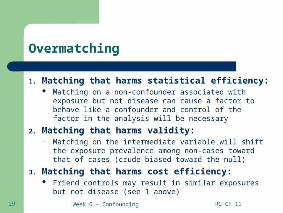
Overmatching

1. Matching that harms statistical efficiency: Matching on a non-confounder associated with exposure but

not disease can cause a factor to behave like a confounder and control of the factor in the analysis will be necessary

2. Matching that harms validity:– Matching on the intermediate variable will shift the exposure

prevalence among non-cases toward that of cases (crude biased toward the null)

3. Matching that harms cost efficiency: Friend controls may result in similar exposures but not

disease (see 1 above)

RG Ch 11


Adjustment for confounding effects of known and measured confounders

Quick review– Methods to adjust for confounding in the analysis stage


Adjustment for confounding effects of known and measured confounders

Quick review– Methods to adjust for confounding in the analysis stage:

Standardization (SMRs and SIRs) Stratification Multivariate analysis

– Selection of important confounders– Adjustment using scoring methods– G-estimation method to adjust for time-varying confounders

RG Ch 21


Adjustment for confounding effects of known and measured confounders: Methods

Stratification shows distributions of key variables and patterns in the data that are less transparent when using other methods; it should be done preliminary to regression methods

– Test of homogeneity of stratum-specific effect estimates Comparison of stratum-specific estimates against a summary estimate obtained by

using – Woolf method or weighted least squares (ample data) – Fisher exact method (sparse data)– ML method (at least 10 cases per stratum)– Mantel-Haenszel method (valid for sparse data but can have much higher variance than

ML) Comparison of observed cell counts against cell counts expected under the

homogeneity hypothesis Both methods have very low power

Multivariate analysis– Confounding variables for the final model could be selected based on the

– change-in-estimate criterion (preferable) – statistical tests (collapsibility testing)– subject matter grounds (“known confounders”)

RG Ch 15


Adjustment for confounding effects of known and measured confounders: Theory: “Comparability” vs. “Collapsibility”

Comparability (Sander Greenland, James Robins, Hal Morgenstern, and Charles Poole) is defined in relation to the counterfactual model for causal inference confounding results from noncomparability, i.e., a difference between the distribution of outcomes for the

unexposed group to what would have been observed in the exposed group if it had not been exposed. Since the latter value is hypothetical and unobservable, the comparability definition cannot be directly applied, though it has some theoretical advantages as well as practical implications.

Collapsibility (D.A. Grayson and others) confounding is present when the crude measure of association differs from the value of that measure

when extraneous variables are controlled by stratification, adjustment, or mathematical modeling readily applied in practice and is widely used makes confounding specific to the measure of association used and the particular variables that are being

controlled

The two definitions generally agree on the presence or absence of confounding when the measure of effect is a ratio or difference of incidences (proportions or rates), but not the odds ratio (unless the situation is one where odds ratio closely estimates a risk or rate ratio, e.g., a rare outcome).


Adjustment for confounding effects of known and measured confounders: Methods, continued

Forward selection step-wise regression method assesses individual effects of confounders, but ignores possible interaction effects between them (joint confounding); it is indicated when data are sparse but in all other situations a backwards deletion strategy should be used

– Read more in A Pocket Guide to Epidemiology, Ch. 11 “Confounding can be confounding – several risk factors.”

RG Ch 15


Sir Richard Doll (American College of Epidemiology Newsletter for Fall 1992)

“There have been many important steps along the way: larger scale studies, more powerful statistical techniques, and the development of computers that allow these techniques to be applied. I fear, however, that the ease of applying statistical packages is sometimes blinding people to what is really going on. You don’t have a real close understanding of what the relationships are when you put environmental and all of the other components of the history together in a logistic regression that allows for fifteen different things. I am a great believer in simple stratification. You know what you are doing, and you really want to look at the intermediate steps and not have all of the data in the computer”.


RCT of tolbutamide in the University Group Diabetes program

Question: The crude value of the risk ratio is 1.44, which is between the values for the risk ratio in the two age strata. Could the crude risk ratio have been outside the range of the stratum-specific values, or must it always fall within the range of the stratum-specific values? Why or why not?

Age Total

<55 55+ <55 55+

Tolbutamide Placebo Tolbutamide Placebo Tolbutamide Placebo

Deaths 8 5 22 16 30 21

Total at risk 106 120 98 85 204 205

Risk Ratio 1.81 1.19 1.44


Question: The larger a randomized trial, the less the possibility for confounding. Why? Explain why size of a study does not affect confounding in nonexperimental studies.


Question: Suppose that an investigator conducting an RCT of an old and a new treatment examines baseline characteristics of the subjects (such as age, sex, stage of disease, and so forth) that might be confounding factors and finds that the two groups are significantly different with respect to several characteristics. A significance test is a test of the null hypothesis, which is a hypothesis that chance alone can account for the observed difference. What is the explanation for baseline differences in a randomized trial? What implication does that explanation have for dealing with these differences?


Scoring methods

Confounder scores are treated as a single confounder in the model:

A categorical compound variable with distinct values for every possible value of measured confounders

Problem: the strata of a compound variable rapidly become too sparse for analysis

Outcome scores are constructed to predict the outcome

Exposure scores also known as propensity scores (Rosenbaum and Rubin 1983)

Criteria for selection of variables in the propensity score should be the same as those used for outcome regression

RG Ch 21


Propensity scores

Propensity score e(x) is defined as conditional exposure probability given a set of observed covariates x

In a cohort study, matching or stratifying treated and controlled subjects on a single variable, the propensity score, tends to balance all of the observed covariates; however, unlike random assignment of treatments, the propensity score may not also balance unobserved covariates.

RG Ch 21


Propensity scores

Could be used for stratification, matching, or as a covariate in the multivariate regression

Stratification or matching on a fitted score requires categorization of propensity score which may introduce residual confounding

RG Ch 21


Propensity scores

Propensity scores are estimated in regression models and range from 0 to 1 and reflect the estimated probability, based on the subject’s characteristics, that the subject will receive the treatment of interest

Any two subjects with the same scores can have different covariate values, but the distributions of covariates for all treated subjects should be similar to those for untreated subjects with the same scores

RG Ch 21


Real-life examples:Hosmer and Lemeshow, 1989

Study of the association between smoking and low birth weight

Other factors: – age of mother, weight at last menstrual period, history of

premature labor, number of physicians visits during first trimester, hypertension, uterine irritability and race

Logistic regression: – Positively associated with smoking: age of mother, history of

premature labor, race (black or white vs. other)– Negatively associated with smoking: weight at last menstrual

period, number of physicians visits during first trimester– Final model should include all of these to obtain an unbiased

estimate of the effect: OR=2.45 (95% CI: 1.15, 5.21)


Real-life examples:Hosmer and Lemeshow, 1989

Propensity score based on selected confounders:– Continuous measure calculated for each study participants, categorized into 5

classes (quintiles)– Direct stratification on all confounders will result in at least 32 sub-classes if all

confounders are dichotomized: OR=1.96 (95%CI: 0.75, 5.20) – Final model included categorical propensity score, other factors were not

associated with smoking, OR=1.61 (95%CI: 0.70, 3.71) – Conclusions:

some residual bias that has not been captured by propensity score Interpretation of the results of logistic regression and regression with propensity scores

is different:– Logistic regression: the odds for a smoker if smoking is ceased while other factors remain

unchanged– Regression with propensity score: the odds due to smoking in a population of smokers when

compared to a population of non-smokers with the same distribution of covariates Logistic regression models individual effect while propensity score analysis estimates

population average


Structural models and G-estimation

Confounders in the model could be:– Endogenous (can be affected by other variables in the model)– Exogenous (cannot be affected by other variables)

– Example:

Y=y0 + b1x1 +b2x2 +b3x3 +b4x4Rate of asthma attacks= baseline (genetic) + endogenous factors (physical activity and medications) + exogenous factors (air pollution and weather)

Multiple causal relations could be modeled with multiple equations (structural-equations modeling)

RG Ch 21


G-estimation in cohort studies

Standard methods for analysis of cohort studies may give biased estimates of exposure effects in the presence of time-varying confounding

Most easily fitted using a two-step procedure called G-estimation

A covariate is a time-varying confounder for the effect of exposure on outcome if

– 1) past covariate values predict current exposure– 2) past exposure predicts current covariate value– 3) current covariate value predicts outcome

RG Ch 21


G-estimation in cohort studies

For each subject, Ui is defined as the time to failure if the subject was unexposed throughout follow-up

Assume no unmeasured confounders conditional on measured history (past and present confounders

and past exposure), present exposure is independent of Ui G-estimation uses the assumption of no unmeasured

confounders to estimate the effect of exposure on survival by examining a range of values for ψ and choosing the value ψ0 for which current exposure is independent of Ui.

Example:– conditional on past weight, smoking status, blood pressure,

and cholesterol, a person’s decision to quit smoking is independent of what his or her survival time would have been if he or she had never smoked


This study examined association between cardiovascular risk factors and all-cause mortality and risk of coronary heart disease (CHD), accounting for confounding between exposures over time which were ascertained through repeated visits. Results were compared with those from standard survival analyses (e.g., Weibull regression) with time-updated covariates. G-estimate adjusted associations differed from those estimated using standard survival analysis. The G-estimated effect of low density lipoprotein and high density lipoprotein cholesterol on CHD incidence were more linear than the standard estimate.


G-estimation in RCTs

In the analysis:– To adjust for noncompliance (nonadherence)– Typical analysis method in the RCT is intent-to-treat– Problem:

Estimates of biologic effects based on intent-to-treat are biased because noncompliance causes assigned treatment to become a misclassified version of received treatment; noncompliers differ from compliers with respect to risk, and therefore conventional analyses of received treatment tend to be confounded

– Solution: Use assigned treatment as a fixed exogenous covariate and received

treatment as an endogenous time-dependent exposure whose effects is represented in a structural nested model

RG Ch 21


Adjustment for confounding effects of known and measured confounders: Caveats

Confounder category boundaries should be chosen in such a way that effect estimates are stable within categories

– particularly important for strong confounders with uneven distributions (percentile categories vs. frequency categories)

Some variables could be both confounders and effect modifiers of the of the exposure-disease association under study

RG Ch 15


Adjustment for confounding effects of known and measured confounders: Caveats, continued

Adjustment for variables that violate any of the criteria for confounding could distort effect estimates (over-adjustment)

– in stratified analysis it can increase the variance and reduce the efficiency of the estimation process

Computed 95% CIs assume that no selection of confounding variables was done. Because they do not reflect the uncertainty about the confounder effects, they may be too narrow

RG Ch 15


Residual confounding

Various adjustment techniques control only for between-stratum confounding, not within-stratum (residual) confounding

What to do: – More strata (categories) with narrower boundaries will control

confounding more effectively than fewer strata (categories) with broader boundaries

– Balance between better adjustment using a lot of strata vs. random error in imprecise estimates from thinly spread data

N.B. The term residual confounding is also used to describe confounding from factors that are not controlled at all or from factors that are controlled but are measured inaccurately


Under- and over-adjustment for confounding effects

Under-adjustment:– If confounders are not identified and not measured– If confounders are identified but not measured– If confounders are identified, but poorly measured (eg., SES,

ethnicity) Over-adjustment:

– Logistic regression can accommodate a lot of confounders, but the results are less transparent and more prone to undetected errors:

– What do estimates mean?– Variance increases with the number of variables in the model– Reduction in precision of risk estimates will make it more difficult to detect

a true association– Effects of some confounders may depend on absence or presence

of other confounders (joint confounding)


Unmeasured confounding

Regardless of our best efforts, there is likely to be some residual confounding in analysis strata. Thus, stratum-specific and summary estimates of associations of exposure with disease and can differ considerably from the stratum-specific and summary effects of exposure on disease. The latter could be estimated by allowing for residual bias.

RG Ch 19


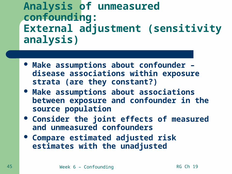
Analysis of unmeasured confounding:External adjustment (sensitivity analysis)

Make assumptions about confounder – disease associations within exposure strata (are they constant?)

Make assumptions about associations between exposure and confounder in the source population

Consider the joint effects of measured and unmeasured confounders

Compare estimated adjusted risk estimates with the unadjusted

RG Ch 19


Analysis of unmeasured confounding:Probabilistic sensitivity analysis (Monte-Carlo simulations)

Extends simple sensitivity analysis by assigning probability distributions to the parameters rather than using a few fixed values for the parameters

At each iteration of a Monte-Carlo analysis, values of the unknown confounder parameters are randomly selected from their assigned probability distributions and then used to produce a frequency distribution of adjusted estimates of the target parameter

2.5% and 97.5% limits of the distribution are the limits of an interval that contains 95% of the simulated estimates (Monte-Carlo simulation interval (MCSI))

Could be additionally adjusted for random error

RG Ch 19


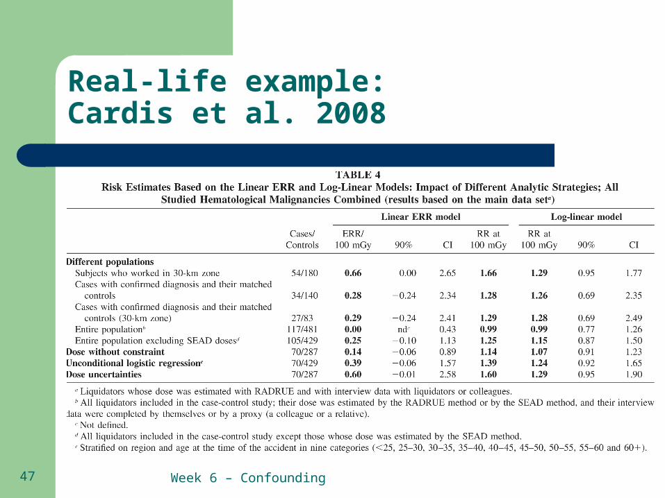
Real-life example:Cardis et al. 2008


Estimating effects of unmeasured confounders and random errors in doses

dose–response models were fitted to each of the 10,000 data sets corresponding to the 10,000 realizations of the doses for each subject. An integrated profile likelihood was then generated by averaging the likelihoods at each of the 100 points over all of the 10,000 simulations, thus providing a MLE and a confidence interval that take into account both the statistical error of the model and the dosimetric uncertainties. dose-response models are fitted 10,000 times as parameter estimates are randomly sampled from their underlying distributions.


Real-life examples:Cardis et al. 2008


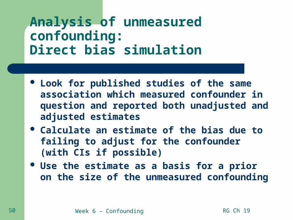
Analysis of unmeasured confounding:Direct bias simulation

Look for published studies of the same association which measured confounder in question and reported both unadjusted and adjusted estimates

Calculate an estimate of the bias due to failing to adjust for the confounder (with CIs if possible)

Use the estimate as a basis for a prior on the size of the unmeasured confounding

RG Ch 19


Summary

Confounding is a distortion or misattribution of effect to a particular study factor. It results from noncomparability of a comparison group.

A confounder should appear as an independent risk factor, i.e., not one whose association with disease results from its association with the study factor. There are multiple caveats to the ‘well-known’ 3 criteria for confounding.

Adequacy of control of confounding effects is compromised by errors in the conceptualization, measurement, coding, and model specification for potential confounders.

Important to remember unmeasured and residual confounding, under- and over-adjustment for confounding effects.

Documents

Week 6 - Confounding 1 C onfounding Lydia B. Zablotska, MD, PhD Associate Professor Department of Epidemiology and Biostatistics