Embed Size (px)
Citation preview
MNRAS 439, 28–47 (2014) doi:10.1093/mnras/stt1946Advance Access publication 2014 February 4
Weighing the Giants – II. Improved calibration of photometry fromstellar colours and accurate photometric redshifts
Patrick L. Kelly,1,2,3,4‹ Anja von der Linden,1,2 Douglas E. Applegate,1,2,3
Mark T. Allen,1,2 Steven W. Allen,1,2,3 Patricia R. Burchat,1,2 David L. Burke,1,3
Harald Ebeling,5 Peter Capak,6 Oliver Czoske,7 David Donovan,5 Adam Mantz8
and R. Glenn Morris1,3
1Kavli Institute for Particle Astrophysics and Cosmology, Stanford University, 452 Lomita Mall, Stanford, CA 94305-4085, USA2Department of Physics, Stanford University, 382 Via Pueblo Mall, Stanford, CA 94305-4060, USA3SLAC National Accelerator Laboratory, 2575 Sand Hill Road, Menlo Park, CA 94025, USA4Department of Astronomy, University of California, Berkeley, CA 94720-3411, USA5Institute for Astronomy, 2680 Woodlawn Drive, Honolulu, HI 96822, USA6California Institute of Technology, MC 249-17, 1200 East California Boulevard, Pasadena, CA 91125, USA7Universitat Wien, Institut fur Astronomie, Turkenschanzstrase 17, A-1180 Wien, Austria8Kavli Institute for Cosmological Physics, University of Chicago, 5640 South Ellis Avenue, Chicago, IL 60637-1433, USA
Accepted 2013 October 8. Received 2013 October 7; in original form 2013 August 1
ABSTRACTWe present improved methods for using stars found in astronomical exposures to calibrateboth star and galaxy colours as well as to adjust the instrument flat-field. By developing aspectroscopic model for the Sloan Digital Sky Survey (SDSS) stellar locus in colour–colourspace, synthesizing an expected stellar locus, and simultaneously solving for all unknownzero-points when fitting to the instrumental locus, we increase the calibration accuracy ofstellar locus matching. We also use a new combined technique to estimate improved flat-fieldmodels for the Subaru SuprimeCam camera, forming ‘star flats’ based on the magnitudes ofstars observed in multiple positions or through comparison with available measurements inthe SDSS catalogue. These techniques yield galaxy magnitudes with reliable colour calibra-tion (�0.01–0.02 mag accuracy) that enable us to estimate photometric redshift probabilitydistributions without spectroscopic training samples. We test the accuracy of our photometricredshifts using spectroscopic redshifts zs for ∼5000 galaxies in 27cluster fields with at leastfive bands of photometry, as well as galaxies in the Cosmic Evolution Survey (COSMOS)field, finding σ ((zp − zs)/(1 + zs)) ≈ 0.03 for the most probable redshift zp. We show that thefull posterior probability distributions for the redshifts of galaxies with five-band photometryexhibit good agreement with redshifts estimated from thirty-band photometry in the COS-MOS field. The growth of shear with increasing distance behind each galaxy cluster showsthe expected redshift–distance relation for a flat � cold dark matter (�-CDM) cosmology.Photometric redshifts and calibrated colours are used in subsequent papers to measure themasses of 51 galaxy clusters from their weak gravitational shear and determine improved cos-mological constraints. We make our PYTHON code for stellar locus matching publicly availableat http://big-macs-calibrate.googlecode.com; the code requires only input catalogues and filtertransmission functions.
Key words: gravitational lensing: weak – methods: observational – techniques: photometric.
1 IN T RO D U C T I O N
A principal challenge for current and planned optical and near-IR wide-field surveys is to estimate accurate redshift probability
� E-mail: [email protected]
distributions for millions of galaxies from broad-band photome-try. Correct probability distributions are necessary, for example, forthe weak-lensing cosmological measurements that current and up-coming surveys (e.g. Dark Energy Survey, Large Synoptic SurveyTelescope) aim to extract from wide-field optical imaging. Pho-tometric redshift algorithms, however, can show significant sys-tematic biases if the input galaxy photometry has even modest
C© 2014 The AuthorsPublished by Oxford University Press on behalf of the Royal Astronomical Society
at California Institute of T
echnology on April 24, 2014
http://mnras.oxfordjournals.org/
Dow
nloaded from
Photometry and photometric redshifts 29
(∼0.03–0.04 mag) calibration error. To infer the weak-lensingmasses of galaxy clusters using photometric redshifts estimatedfrom Subaru and Canada–France–Hawaii telescope (CFHT) pho-tometry, we have developed and applied several techniques to cali-brate broad-band galaxy colours to an accuracy of ∼0.01–0.02 mag,without requiring specific standard star observations.
The relative distribution of counts recorded during flat-field expo-sures of an illuminated screen or of the sky can differ from the actualinstrument sensitivity by up to ∼10 per cent across the focal plane(Manfroid, Selman & Jones 2001; Koch et al. 2003; Magnier &Cuillandre 2004; Capak et al. 2007; Regnault et al. 2009) becauseof a combination of geometric distortion, superposed reflections,and imperfect flat-field sources. We combine two methods to mea-sure the Subaru SuprimeCam ‘star flat’, the map of the spatiallydependent zero-point error that remains after traditional flat-fieldcorrection, across a decade of observations and camera upgrades.Our star-flat model is informed by the magnitudes of the same starsobserved in multiple locations on the focal plane, as well as bycomparisons with available SDSS catalogue magnitudes.
A powerful colour calibration strategy suitable for use withmedium-to-wide-field data uses the fact that almost all of the starsobserved in any field lie along a well-understood one-dimensionallocus in colour–colour space (e.g. MacDonald et al. 2004; Highet al. 2009). According to this technique, the zero-points of thefilters are shifted until the position of the observed stellar locusmatches the expected locus. The resulting calibration automaticallycorrects for Milky Way dust extinction. We improve the accuracy ofthis technique by constructing a spectroscopic model for the SDSSstellar locus, and by developing a numerical algorithm that fits forall unknown zero-points simultaneously.
Comparison of photometric redshifts estimated from our cali-brated galaxy magnitudes against spectroscopic redshifts show thatthese bootstrapped calibration techniques are effective. We find ex-cellent agreement between the most probable photometric redshiftzp and the spectroscopic redshift zs, with a measurement error ofσ ((zp − zs)/(1 + zs)) ≈ 0.03. Five-band p(z) distributions summedover different sets of galaxies (
∑galp(z)) show congruence with the
Ilbert et al. (2009) 30-band photometric redshift distributions for thesame sets of galaxies. The growth of lensing shear with increasingredshift of galaxies behind each cluster, sensitive to the photomet-ric redshifts of galaxies too faint to be represented in spectroscopicsamples, exhibits the shape expected for a flat � cold dark matter(�-CDM) cosmology.
The algorithms and techniques described in this paper may beuseful as a primary means of calibration or as a demanding test ofzero-point accuracy. This paper is the second in a series (‘Weigh-ing the Giants’) addressing the specific task of measuring accurategalaxy-cluster masses using shear-based weak-lensing methods.Paper I (von der Linden et al. 2014) in this series describes theoverall project strategy, the cluster sample and the data reductionmethods. Paper III (Applegate et al. 2014) presents a Bayesianapproach to measuring galaxy-cluster masses, that uses the fullphotometric redshift probability distributions reported here; thesemasses are compared to those measured with a standard ‘colour-cut’method based on three-filter photometry for each field.
Section 2 of this paper summarizes the wide-field imaging dataused here. In Section 3, we describe how we determine the Suprime-Cam star flats, which we use to extract consistent magnitudesacross the CCD array. Section 4 describes the stellar locus cali-bration algorithm and the spectroscopic model we have developedfor the stellar locus. In Section 5, we discuss the algorithms andthe templates for galaxy spectra that we use to estimate photometric
redshift probability distributions p(z). A method for finding the zero-points of u∗- and BJ-band photometry is presented in Section 6. InSection 7, we use the galaxy-cluster red sequence and spectroscopicredshift measurements in the cluster fields to evaluate the accuracyof our photometric calibrations and redshift estimates. In Section7.3, we compare the redshift probability distributions determinedfrom calibrated photometry in five bands (BJVJr+i+z+) against boththe zCOSMOS spectroscopic redshift sample and the most probableredshift inferred from 30 imaging bands in the Cosmic EvolutionSurvey (COSMOS) field. General agreement between the observedgrowth of weak-lensing shear with distance behind the massiveclusters and the �-CDM expectation is found in Section 8. In Sec-tion 9, we summarize the calibration techniques and the quality ofthe photometric redshift estimates.
2 SU BA RU A N D C F H T I M AG I N G DATA
Our imaging data set consists of wide-field optical exposures of51 X-ray-luminous galaxy clusters that span the redshift interval0.15 < z < 0.7. The data were acquired between 2000 and 2009with SuprimeCam mounted on the 8.3-metre Subaru telescope andwith MegaPrime on the 3.6-metre CFHT. The field of view ofSuprimeCam is 34 arcmin × 27 arcmin (0.2 arcsec pixel−1), whilethe MegaPrime has a 1◦ × 1◦ field of view (0.187 arcsec pixel−1).Each cluster field was imaged in at least three separate broad-bandfilters, and 27 fields were imaged with five or more SuprimeCam(BJVJRCICz+) or MegaPrime (u∗g∗r∗i∗z∗) bandpasses. Paper I de-scribes the cluster sample and observations, the overscan, bias, anddark corrections, as well as the flat-field and superflat processingsteps.
3 M E A S U R I N G T H E STA R FL AT
The intensity of a pixelated image recorded by a CCD cameramounted on a telescope depends, in part, on the properties of theCCD sensors and the readout electronics, as well as the illumina-tion of the focal plane by the telescope optics. Correcting imagesfor spatial sensitivity variations is necessary to be able to extractaccurate fluxes for galaxies and stars.
Calibration images of illuminated dome screens, the twilight skyand the night sky vary smoothly on scales of tens of arcseconds, andthese exposures of flat-field sources are useful for measuring localpixel-to-pixel sensitivity variations. The variation of ‘flat-field’ im-ages taken with a wide-field camera on several arcminute scales,however, can disagree with the camera’s actual sensitivity to pointsources. The discrepancy can be up to ∼10 per cent across the fieldof view of wide-field instruments (Manfroid et al. 2001; Koch et al.2003; Magnier & Cuillandre 2004; Capak et al. 2007; Regnaultet al. 2009). Dividing wide-field science images by flat-field ex-posures leads to objects near the centre of the focal plane that aresystematically fainter than sources at the periphery.
Geometric distortion along the optical paths of many wide-fieldtelescopes, such as Subaru/SuprimeCam and CFHT/MegaPrime,results in a decrease in pixel scale with increasing distance from thecentre of the focal plane. In SuprimeCam, the pixel scale decreasesby ∼1.5 per cent between the centre and 15 arcmin from the centre,with a corresponding decrease of ∼3 per cent in the solid anglesubtended by a pixel. (See fig. 3 in Paper I.) This effect means thatpixels near the centre of the field will receive proportionally greaterflux than they otherwise would when illuminated by a hypotheticalcalibration source with constant flux per unit solid angle. The effectof variation in pixel solid angle due to geometric distortion can be
MNRAS 439, 28–47 (2014)
at California Institute of T
echnology on April 24, 2014
http://mnras.oxfordjournals.org/
Dow
nloaded from
30 P. L. Kelly et al.
explicitly corrected using the Jacobian of the astrometric distortion(e.g. Capak et al. 2007), or left for correction by a ‘star flat’ (e.g.Regnault et al. 2009), which is the approach we take.
Light that scatters off the surfaces of reflective and refractiveoptical elements also contributes to the spatial distribution of countsin flat-field images. On average, photons scattering from filtersand the CCD sensors are redirected towards the field centre (e.g.Regnault et al. 2009). This can be seen, for example, in the haloesthat surround bright stars. Stellar haloes, which are due to extrareflections, are each centred on a point that is offset from the startowards the centre of the field of view. For diffuse sources thatextend across the field of view, such as dome screens or the nightsky, a continuum of superposed reflections accumulates near thecentre of the exposure.
Light baffles for wide-field instruments can only be modestly ef-fective. Capak et al. (2007) showed that the intensity of a Suprime-Cam flat-field varies by ±5 per cent in the corners of the focal planedue to light scattered from outside the field of view and that theintensity of scattered light depends on the position of the telescopeand whether exposures were taken in dark or twilight conditions. Toreduce our susceptibility to these intensity variations in the periph-ery, we exclude regions of the sensors that are more than 15 arcminfrom the centre of the field.
Zero-point variations across the focal plane that remain after di-viding images by flat-field exposures can be measured with twoapproaches. A first technique is to image the same set of stars atdifferent positions in the focal plane by dithering the telescope orrotating the camera, and find the spatially dependent corrections(the ‘star flat’) that result in the smallest dispersion in magnitudesfor each star measured in different positions (Manfroid et al. 2001;Magnier & Cuillandre 2004; Capak et al. 2007; Padmanabhan et al.2008; Regnault et al. 2009; Wittman, Ryan & Thorman 2012). Asecond approach is to compare the measured magnitudes of stars tothose in photometrically consistent catalogues, such as the SDSScatalogues (Koch et al. 2003). We apply both approaches and de-scribe the process in detail below.
The CFHT ELIXIR pipeline fits and corrects for a star flat forMegaPrime observations (Magnier & Cuillandre 2004), so we mea-sure only the SuprimeCam star flat across nine years of observa-tions. In addition to spatially varying zero-point corrections, Reg-nault et al. (2009) find evidence for position-dependent colour termsacross the CFHT MegaPrime field of view, which the authors at-tribute to an angular dependence of the transmission function forinterference filters.
3.1 Chip configurations: SuprimeCam sensorand electronics upgrades
We have grouped our 2000–2009 SuprimeCam images into suc-cessive periods that correspond to upgrades of the CCD array (seetable 3 of Paper I). The CCD sensors in the early 8- and 9-chipconfigurations exhibited non-linear response. We were able to cor-rect the non-linearity except for two MIT/Lincoln CCD sensors inconfiguration 8 and three MIT/Lincoln CCD sensors in configura-tion 9, which we discarded. The ‘10_1’ and ‘10_2’ configurations,installed 2001 March 27, feature 10 MIT/Lincoln CCD sensors withfewer cosmetic defects and linear response below saturation. Theupper-left chip had lower quantum efficiency than the other CCDs,but this can be corrected by the flat field. The last set, the ‘10_3’configuration installed in 2008 July, consists of 10 Hamamatsu Pho-tonics CCD sensors.
3.2 Flat-field correction applied to Subaru imaging
Before fitting for the SuprimeCam star flat, we divide each image bya stack of dome-flat or twilight-flat exposures taken during the sameobserving run (or adjacent runs if few flats are available), and thenby a heavily smoothed stack of night-sky flats (or ‘superflat’). Flatimages are normalized by their median pixel value before beingstacked. The night-sky flat is constructed from object-subtracted,smoothed exposures, already divided by the stacked dome or twi-light flats, with no bright stars or strong internal reflections (seeErben et al. 2005) and typically varies by (0.5–1.5) per cent acrossthe field of view. While the stack of dome-flat or twilight-flat ex-posures corrects pixel-to-pixel sensitivity variations, the smoothednight-sky superflat makes adjustments for larger scale features.
3.3 Dither patterns and camera rotations
Telescope dithers or camera rotations that move stars substantialdistances across the focal plane are helpful to constrain spatialzero-point variation. The 34 arcmin × 27 arcmin SuprimeCamexposures that we analyse have dither patterns that generally varyby a relatively modest angle of 1–2 arcmin. For Subaru images thatwe took to measure the masses of the MACS (Ebeling, Edge &Henry 2001; Ebeling et al. 2007, 2010) galaxy clusters, we rotatedthe camera by 90◦ to facilitate star-flat fits. Subaru images thatwere taken by other groups and included in our analysis, whichwe accessed through the Subaru–Mitaka–Okayama–Kiso Archive(SMOKA)1 (Baba et al. 2002), can have different dither sequencesand rotations (e.g. rotations of 45◦ or no rotation).
3.4 Measuring the star flat
We perform a separate star-flat fit to each of 471sets of exposurescorresponding to a given cluster field, filter and observing run (e.g.Abell 68, BJ, 2007 July 18). The median number of exposures weuse for each star-flat fit is six, with a typical relative rotation of 90◦
after the first three exposures.
3.4.1 Selecting the star sample
To select stars, we choose objects that the SEXTRACTOR (Bertin &Arnouts 1996) neural network classifier, supplied with the im-age seeing (SEEING_FWHM), suggests are stellar-like (i.e. whereCLASS_STAR > 0.65). We also admit only those star candidatesfor which the flux within 2.5 Kron (1980) radii (MAG_AUTO) hasless than 0.1 mag uncertainty, as well as where the stellar image isunblended, has no bad or saturated pixels, has no bright neighboursand is not truncated by a CCD sensor boundary (i.e. we includeonly objects with FLAG = 0). To exclude objects that are saturatedor affected by detector non-linearity in our images, we include onlymeasurements of objects with a maximum pixel value less than25 000 ADU above the ∼10 000 ADU bias level, well below thefull-well capacity of ∼35 000 ADU above the bias level. Both forfitting the star flats and for measuring galaxy photometry and shapesfor the analysis of weak lensing, we exclude objects in each cat-alogue that are more than 15 arcmin from the centre of the field.To identify and remove exceptionally discrepant magnitudes early,we use objects that appear in different exposures to estimate therelative zero-point of each exposure, and subtract these zero-points
1 http://smoka.nao.ac.jp/
MNRAS 439, 28–47 (2014)
at California Institute of T
echnology on April 24, 2014
http://mnras.oxfordjournals.org/
Dow
nloaded from
Photometry and photometric redshifts 31
from the magnitude measured for each object. For each star can-didate, we remove any magnitude measurements m
expstar for which
|mexpstar − median(m)| > 1 mag, where median(m) is the median of
magnitudes mexpstar across all exposures.
3.4.2 Star-flat model
We model the SuprimeCam position-dependent zero-point with aspatially varying function C(x, y, chip, rotation), which is the sumof a separate function f(x, y)rot for each rotation of the cameraand a single set of chip-dependent offsets Ochip, shared across therotations and dithered exposures:
C(x, y, chip, rotation) = f (x, y)rot + Ochip, (1)
where f (x, y)rot is the product of third-order Chebyshev polynomialsin x and y coordinates on the focal plane.
For the stars in each exposure that meet the sample criteria, weexpress the measured magnitude of each star, m
expstar, in terms of the
spatially varying correction C(x, y, chip, rotation), and a magnitudemmodel
star , which is a free parameter in the fit and corresponds to thestellar magnitude that would be measured if the exposures had noposition-dependent zero-point variation:
mexpstar = C(x, y, chip, rotation) + ZPexp + mmodel
star , (2)
where ZPexp is the zero-point for each exposure.We also introduce constraints from available magnitudes from
photometrically consistent catalogues. These are SDSS magnitudesor, alternatively, SuprimeCam or MegaPrime magnitudes correctedby a previous successful star-flat fit. We express each available cat-alogue magnitude mcat
star in terms of the modelled magnitude mmodelstar ,
a zero-point offset Ocat, and a colour term Scat × ccatstar:
mcatstar = mmodel
star + Ocat − Scat × ccatstar. (3)
The star colour ccatstar is calculated from catalogue magnitudes (e.g.
g′ − r′). We find the coefficient Scat of the colour term before fittingfor the other star-flat parameters.
The free parameters in the model are the coefficients in the Cheby-shev polynomials in f (x, y)rot for each camera rotation, Ochip, Ocat,ZPexp, and, for each star, mmodel
star .
3.4.3 Fitting procedure
We construct a set of linear equations from two sets of equations:equation (2) for each observation of each stellar candidate, andequation (3) for each star with a catalogue magnitude. The matrixrepresenting the system of equations where each equation corre-sponds to a row is sparse because only a handful of equationsinclude mmodel
star for each star. Each row in the matrix is weightedby the inverse-square of the uncertainty in m
expstar or mcat
star. When thestatistical uncertainty is less than 0.04 mag, we set the uncertainty tobe 0.04 mag for purposes of the fit, so that a small number of objectswill not dominate the solution. We use CXSparse (Davis 2006), aC library for sparse matrix algebra, to apply a QR decompositioncomputed with a Householder transformation.
After computing an initial solution, measured magnitudes mexpstar
that are more than 5σ from the corresponding model magnitudesmmodel
star are removed. We then refit the remaining measured andcatalogue magnitudes, m
expstar and mcat
star.When fewer than 400 stars in the exposure have a catalogue mag-
nitude mcatstar, we remove linear terms in the Chebyshev polynomials
in f(x, y)rot because the set of exposure zero-points Ochip exhibit a
degeneracy with the linear Chebyshev terms. Consider, for example,exposures taken after three successive telescope dithers to the northby 1 arcmin. If all stars show fluxes that diminish by 10 per centwith each consecutive exposure, these changes in flux could reflecteither worsening atmospheric transparency (i.e. ZPexp) or a linearspatial gradient in the camera’s sensitivity. The addition of a suffi-cient number of mcat
star magnitudes from an external photometricallyconsistent catalogue for stars spanning the field of view, however,breaks this degeneracy.
3.4.4 Evaluating the star-flat fit to each set of exposures
To identify star-flat solutions that have small statistical uncertaintyand are robust to outliers, we calculate a statistic, which we call σ jack,using star-flat fits to 10 separate jackknife samples, each containinga randomly selected set of half the stars. The statistic, σ jack, is ameasure of the variation in the star-flat solution across the samples.
We create a pixelated image of the best-fitting star-flat model (inmagnitudes) across the focal plane for each jackknife sample, whereeach pixel cell corresponds to an area of 20 arcsec × 20 arcsec, or100 × 100 CCD pixels. Each jackknife correction map can then berepresented by An
ij , where i and j are the pixel coordinates, n denotesthe nth jackknife sample and An
ij is the mean of the star-flat modelwithin pixel (i, j). We use the An
ij maps to assess the uncertainty ofthe star-flat fits. Since we are interested only in the relative spatiallyvarying corrections, we subtract the median correction across theimage from the correction in each pixel: δAn
ij = Anij − median(An).
We then calculate the standard deviation σ (δAij) for each pixelacross the jackknife fits.
To assess the uncertainty of the correction calculated from eachstar flat, we use the median of σ (δAij) across all pixels in the image,which we call σ jack.
3.4.5 Required value of σ jack
Selecting a maximum acceptable value for σ jack presents a tradeoffbetween two objectives. On the one hand, we want to measure thestar flat for as many observing runs and pointings as possible tocorrect for any variation with position in the sky and with time.On the other hand, we want to apply a correction only when thestatistical uncertainty on the correction is small. We adopted thecriteria outlined in the following paragraph but, as shown in Table 1,the average values of the σjack statistic for each chip configurationare substantially better than these thresholds.
For chip configurations 8 and 9 (see Section 3.1), the minimal re-quirement for using the star-flat correction is that σ jack < 0.03 mag(i.e. star flat constrained to ∼0.03 mag). For chip configurations10_1, 10_2 and 10_3, where greater numbers of objects are gener-ally available, we consider a fit acceptable if σ jack < 0.01 mag. Weattempted star-flat fits to 471 sets, and 183 of the solutions satisfiedthese requirements.
A star-flat solution may be too poorly constrained to meet theminimal σ jack requirement for several reasons. These include lowstellar density in the galaxy-cluster field, exposures taken withoutcamera rotation, no overlap with the SDSS footprint and minimaltelescope dithers between exposures. When the star-flat fit does notmeet the σ jack criterion, we look for a satisfactory star flat for adifferent filter of the same field and use the corrected mmodel
star mag-nitudes as reference mcat
star magnitudes. When even these additionalconstraints from mcat
star do not yield an acceptable solution, we cor-rect the data by the satisfactory star flat for data taken closest intime (with the same filter and chip configuration).
MNRAS 439, 28–47 (2014)
at California Institute of T
echnology on April 24, 2014
http://mnras.oxfordjournals.org/
Dow
nloaded from
32 P. L. Kelly et al.
Table 1. Diagnostic fit statistics averaged across acceptable star flats, sorted by chipconfiguration and whether SDSS stellar photometry was available for at least 400 matchedstellar objects. The statistic 〈σ jack〉 shows that the star-flat correction is well constrained.
Chip configuration SDSS matches Cluster/Filter/Run combinations 〈σ jack〉
10_3 None 3 0.003 mag10_3 Yes 4 0.003 mag
10_1 & 10_2 None 69 0.004 mag10_1 & 10_2 Yes 96 0.003 mag
8 & 9 None 6 0.009 mag8 & 9 Yes 5 0.021 mag
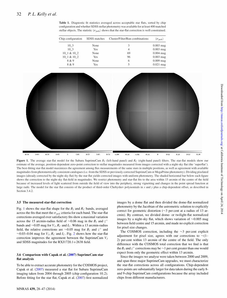
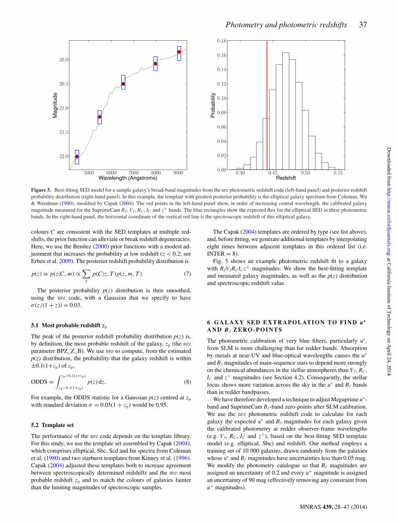
Figure 1. The average star-flat model for the Subaru SuprimeCam BJ (left-hand panel) and RC (right-hand panel) filters. The star-flat models show ourestimate of the average, position-dependent zero-point correction to stellar magnitudes measured from images corrected with a night-sky flat (the ‘superflat’).The best-fitting star-flat model maximizes the agreement among flux measurements of the same stars in multiple positions, as well as agreement with availablemagnitudes from photometrically consistent catalogues (i.e. from the SDSS or previously corrected SuprimeCam or MegaPrime photometry). Dividing pixelatedimages (already corrected by the night-sky flat) by the star flat yields corrected images with uniform photometry. The shaded horizontal bar below each figureshows the correction to the night-sky flat-field in magnitudes. We restrict photometry and star-flat fits to the area within 15 arcmin of the centre of the fieldbecause of increased levels of light scattered from outside the field of view into the periphery, strong vignetting and changes in the point spread function atlarge radii. The model for the star flat consists of the product of third-order Chebyshev polynomials in x and y plus a chip-dependent offset, as described inSection 3.4.2.
3.5 The measured star-flat correction
Fig. 1 shows the star-flat shape for the BJ and RC bands, averagedacross the fits that meet the σ jack criteria for each band. The star-flatcorrections averaged over satisfactory fits show a maximal variationacross the 15 arcmin-radius field of ∼0.06 mag in the BJ and z+
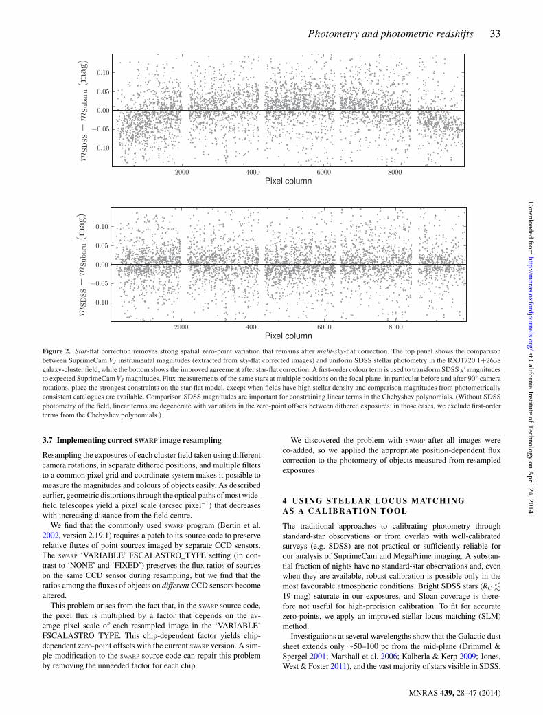
bands and ∼0.05 mag for VJ, RC and IC. Within a 13 arcmin-radiusfield, the relative corrections are ∼0.05 mag for BJ and z+ and∼0.03–0.04 mag for VJ, RC and IC. Fig. 2 shows how the star-flatcorrection improves the agreement between the SuprimeCam VJ
and SDSS magnitudes for the RXJ1720.1+2638 field.
3.6 Comparison with Capak et al. (2007) SuprimeCam starflat analysis
To be able to extract accurate photometry for the COSMOS project,Capak et al. (2007) measured a star flat for Subaru SuprimeCamimaging taken from 2004 through 2005 (chip configuration 10 2).Before fitting for the star flat, Capak et al. (2007) first normalized
images by a dome flat and then divided the dome-flat normalizedphotometry by the Jacobian of the astrometric solution to explicitlycorrect for geometric distortion (∼3 per cent at a radius of 13 ar-cmin). By contrast, we divided dome- or twilight-flat normalizedimages by a night-sky flat, which shows variation of ∼0.005 magbetween field centre and 15 arcmin, and made no explicit correctionfor pixel size changes.
The COSMOS correction, including the ∼3 per cent explicitadjustment for pixel size, agrees with our corrections to ∼(1–2) per cent within 13 arcmin of the centre of the field. The onlydifference with the COSMOS total correction that we find is thatthe BJ and z+ corrections may be ∼1 per cent greater than one wouldexpect from only the geometric effect within 13 arcmin.
Since the images we analyse were taken between 2000 and 2009,and span three major SuprimeCam upgrades, we must characterizethe star-flat corrections across all configurations. Chip-dependentzero-points are substantially larger for data taken during the early 8-and 9-chip SuprimeCam configurations because the array includedchips from different manufacturers.
MNRAS 439, 28–47 (2014)
at California Institute of T
echnology on April 24, 2014
http://mnras.oxfordjournals.org/
Dow
nloaded from
Photometry and photometric redshifts 33
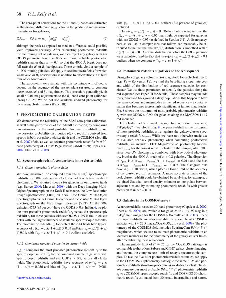
Figure 2. Star-flat correction removes strong spatial zero-point variation that remains after night-sky-flat correction. The top panel shows the comparisonbetween SuprimeCam VJ instrumental magnitudes (extracted from sky-flat corrected images) and uniform SDSS stellar photometry in the RXJ1720.1+2638galaxy-cluster field, while the bottom shows the improved agreement after star-flat correction. A first-order colour term is used to transform SDSS g′ magnitudesto expected SuprimeCam VJ magnitudes. Flux measurements of the same stars at multiple positions on the focal plane, in particular before and after 90◦ camerarotations, place the strongest constraints on the star-flat model, except when fields have high stellar density and comparison magnitudes from photometricallyconsistent catalogues are available. Comparison SDSS magnitudes are important for constraining linear terms in the Chebyshev polynomials. (Without SDSSphotometry of the field, linear terms are degenerate with variations in the zero-point offsets between dithered exposures; in those cases, we exclude first-orderterms from the Chebyshev polynomials.)
3.7 Implementing correct SWARP image resampling
Resampling the exposures of each cluster field taken using differentcamera rotations, in separate dithered positions, and multiple filtersto a common pixel grid and coordinate system makes it possible tomeasure the magnitudes and colours of objects easily. As describedearlier, geometric distortions through the optical paths of most wide-field telescopes yield a pixel scale (arcsec pixel−1) that decreaseswith increasing distance from the field centre.
We find that the commonly used SWARP program (Bertin et al.2002, version 2.19.1) requires a patch to its source code to preserverelative fluxes of point sources imaged by separate CCD sensors.The SWARP ‘VARIABLE’ FSCALASTRO_TYPE setting (in con-trast to ‘NONE’ and ‘FIXED’) preserves the flux ratios of sourceson the same CCD sensor during resampling, but we find that theratios among the fluxes of objects on different CCD sensors becomealtered.
This problem arises from the fact that, in the SWARP source code,the pixel flux is multiplied by a factor that depends on the av-erage pixel scale of each resampled image in the ‘VARIABLE’FSCALASTRO_TYPE. This chip-dependent factor yields chip-dependent zero-point offsets with the current SWARP version. A sim-ple modification to the SWARP source code can repair this problemby removing the unneeded factor for each chip.
We discovered the problem with SWARP after all images wereco-added, so we applied the appropriate position-dependent fluxcorrection to the photometry of objects measured from resampledexposures.
4 U S I N G S T E L L A R L O C U S M AT C H I N GA S A C A L I B R AT I O N TO O L
The traditional approaches to calibrating photometry throughstandard-star observations or from overlap with well-calibratedsurveys (e.g. SDSS) are not practical or sufficiently reliable forour analysis of SuprimeCam and MegaPrime imaging. A substan-tial fraction of nights have no standard-star observations and, evenwhen they are available, robust calibration is possible only in themost favourable atmospheric conditions. Bright SDSS stars (RC �19 mag) saturate in our exposures, and Sloan coverage is there-fore not useful for high-precision calibration. To fit for accuratezero-points, we apply an improved stellar locus matching (SLM)method.
Investigations at several wavelengths show that the Galactic dustsheet extends only ∼50–100 pc from the mid-plane (Drimmel &Spergel 2001; Marshall et al. 2006; Kalberla & Kerp 2009; Jones,West & Foster 2011), and the vast majority of stars visible in SDSS,
MNRAS 439, 28–47 (2014)
at California Institute of T
echnology on April 24, 2014
http://mnras.oxfordjournals.org/
Dow
nloaded from
34 P. L. Kelly et al.
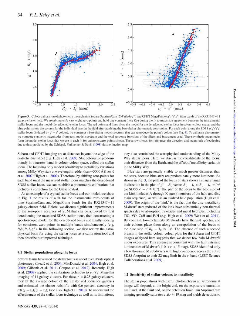
Figure 3. Colour calibration of photometry through nine Subaru SuprimeCam (BJVJRCICz+) and CFHT MegaPrime (g∗r∗i∗z∗) filter bands of the RXJ1347−11galaxy-cluster field. We simultaneously vary eight zero-points and hold one constant (here RC) during the fit to maximize agreement between the instrumentalstellar locus and the model (dereddened) stellar locus. The red points and lines show the model for the dereddened stellar locus in colour–colour space, and theblue points show the colours for the individual stars in the field after applying the best-fitting photometric zero-points. For each point along the SDSS u′g′r′i′z′stellar locus (indexed by g′ − i′ colour), we construct a best-fitting model spectrum that can reproduce the point’s colour (see Fig. 4). To calibrate photometry,we compute synthetic magnitudes from each model spectrum and the total response functions of the filters and instrument used. These synthetic magnitudesform the model stellar locus that we use in each fit for unknown zero-points shown. The arrow shows, for reference, the direction and magnitude of reddeningdue to dust predicted by the Schlegel, Finkbeiner & Davis (1998) dust extinction map.
Subaru and CFHT imaging are at distances beyond the edge of theGalactic dust sheet (e.g. High et al. 2009). Star colours lie predom-inantly in a narrow band in colour–colour space, called the stellarlocus. The locus has only modest sensitivity to metallicity variationsamong Milky Way stars at wavelengths redder than ∼5000 Å (Ivezicet al. 2007; High et al. 2009). Therefore, by shifting zero-points foreach band until the measured stellar locus matches the dereddenedSDSS stellar locus, we can establish a photometric calibration thatincludes a correction for the Galactic dust.
As an example of a typical stellar locus and our model, we showin Fig. 3 the results of a fit for the instrumental zero-points ofnine SuprimeCam and MegaPrime bands for the RXJ1347−11galaxy-cluster field. Below, we discuss significant improvementsto the zero-point accuracy of SLM that can be achieved by firstdereddening the measured SDSS stellar locus, then constructing aspectroscopic model for the dereddened locus and finally, solvingfor consistent zero-points in multiple bands simultaneously (e.g.BJVJRCICz+). In the following section, we first review the astro-physical basis for using the stellar locus as a calibration tool andthen describe our improved technique.
4.1 Stellar populations along the locus
Several teams have used the stellar locus as a tool to calibrate opticalphotometry (Ivezic et al. 2004; MacDonald et al. 2004; High et al.2009; Gilbank et al. 2011; Coupon et al. 2012). Recently, Highet al. (2009) applied the calibration technique to g′r′i′z′ Magellanimaging of 11 galaxy clusters. For these z < 0.25 galaxy clusters,they fit the average colour of the cluster red sequence galaxiesand estimated the cluster redshifts with 0.6 per cent accuracy inσ ((zp − zs)/(1 + zs)) (see also High et al. 2010). To understand theeffectiveness of the stellar locus technique as well as its limitations,
they also scrutinized the astrophysical understanding of the MilkyWay stellar locus. Here, we discuss the constituents of the locus,their distances from the Earth, and the effect of metallicity variationin the Milky Way.
Blue stars are generally visible to much greater distances thanred stars, because blue stars are predominately more luminous. Asshown in Fig. 3, the path of the locus of stars shows a sharp changein direction in the plot of g∗ − RC versus RC − IC at RC − IC ≈ 0.6(or SDSS r′ − i′ ≈ 0.7). The part of the locus to the blue side ofthe kink includes A through K stars (members of the halo and discmain sequence), as well as an evolved halo population (High et al.2009). The origin of the ‘kink’ is the fact that the disc-metallicityM-dwarf stars redward of the kink have substantially non-thermalspectra due to absorption by oxides and metal hydrides, includingTiO, VO, CaH and FeH (e.g. High et al. 2009; West et al. 2011).By contrast, low-metallicity M dwarfs have thermal spectra, andtheir colours place them along an extrapolation of the locus tothe blue side of RC − IC ≈ 0.6. The absence of such a secondbranch in the stellar colour–colour plots for the Subaru and CFHTimages analysed here suggests that we detect few halo M dwarfsin our exposures. This absence is consistent with the faint intrinsicluminosities of M dwarfs (10 < r < 15 mag). SDSS identified onlya few thousand M subdwarfs with high confidence across the entireSDSS footprint to their 22-mag limit in the r′ band (LSST ScienceCollaborations et al. 2009).
4.2 Sensitivity of stellar colours to metallicity
The stellar populations with useful photometry in an astronomicalimage will depend, at the bright end, on the exposure’s saturationlimit and, at the faint end, on the detection limit. Our SuprimeCamimaging generally saturates at RC ≈ 19 mag and yields detections to
MNRAS 439, 28–47 (2014)
at California Institute of T
echnology on April 24, 2014
http://mnras.oxfordjournals.org/
Dow
nloaded from
Photometry and photometric redshifts 35
RC ≈ 26 mag. For SDSS exposures, the range of useful magnitudesin r′ is between ∼14 and ∼22.5 mag.
Catalogues made from deeper exposures will include a higherfraction of halo members in the stellar locus to the blue side ofthe kink in the colour–colour plot in Fig. 3(a). Although stars with0.2 < g − r < 0.4 are approximately evenly split between thedisc and halo populations at SDSS depths, our Subaru and CFHTcatalogues contain a higher fraction of halo stars, given the deeperlimiting magnitudes. Since we use the SDSS stellar locus as a modelfor the locus in our deeper Subaru and CFHT exposures, we needto consider whether the properties of the stellar locus may changewith a larger population of halo-metallicity main-sequence stars.
Using SDSS photometry and spectroscopy, Ivezic et al. (2008)find that the halo population has a Gaussian metallicity distribu-tion with mean [Fe/H]halo ≈ −1.5, while the metallicity of discstars decreases with distance Z from the mid-plane according to[Fe/H]disc = (−0.78 + 0.35, exp(−|Z|, kpc−1)) dex.
High et al. (2009) use model stellar atmospheres to study howthe metallicity difference between the disc and halo main-sequencepopulations affects the colour of their stellar population. They as-sign a metallicity of [Fe/H] = −0.5 for the disc population and ametallicity of [Fe/H] = −1.5 for the halo population. The differencein g′ − r′ colour for main-sequence stars in the two populations, inthe region of the stellar locus to the blue end of the kink, is only∼0.01 mag. However, the u′ − g′ colours for the disc main-sequencestars are ∼0.1 mag redder than those for their halo counterparts.
For this reason, we elect not to use the stellar locus to cali-brate near-UV bands for our ‘Weighing the Giants’ study of Subaruand CFHT imaging. Near-UV emission of stars has comparativelystrong sensitivity to the difference between halo and disc metallici-ties (High et al. 2009), and the SDSS u′-band filter leak near 7100Å additionally affects measurements of the stellar locus in coloursthat include the u′ band. There are, however, strategies that mayenable use of the stellar locus measured from SDSS magnitudes tocalibrate near-UV photometry in future efforts.
4.3 SDSS stellar locus corrected for extinction
We measure the stellar locus from SDSS Data Release 8 (Aiharaet al. 2011) photometry corrected for Galactic dust extinction. Starsare drawn from fields with comparatively low Galactic extinction(AV < 0.2 mag) and their magnitudes corrected by the Schlegel et al.(1998) extinction map. We place stars into bins according to theirg′ − i′ colour (a proxy for effective temperature) and, for a seriesof colours (e.g. g′ − r′, r′ − i′), measure the median stellar colourwithin each bin following the general approach used by Covey et al.(2007).
High et al. (2009) instead used the Covey et al. (2007) stellarlocus, which is not corrected for extinction by Milky Way dust. Wefind that g′ − z′ locus colour and photometric calibration changeby ∼0.05 mag after correcting the stellar locus for Milky Wayextinction.
4.4 Defining model spectra along the locus
The broad-band filters used for the Subaru and CFHT observations,especially the SuprimeCam BJVJRCIC bandpasses, have substan-tially different transmission functions than SDSS u′g′r′i′z′ filters.The colour transformations are non-linear, and we found that a sim-ple, linear colour term yielded poor zero-point solutions. To performimproved colour transformations between magnitudes in differentfilter sets, we construct a comprehensive spectroscopic model for
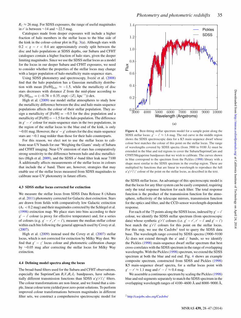
Figure 4. Best-fitting stellar spectrum model for a sample point along theSDSS stellar locus: g′ − i′ ≈ 1.6 mag. The red curve in the middle regionshows the SDSS spectroscopic data for a K5 main-sequence dwarf whosecolour best matches the colour of this point on the stellar locus. The rangeof wavelengths covered by SDSS spectra (from 3900 to 9100 Å) must beextended in the blue and red regions to cover the Subaru/SuprimeCam andCFHT/Megaprime bandpasses that we wish to calibrate. The curves shownin blue correspond to the spectrum from the Pickles (1998) library with ashape most similar to the SDSS spectrum in the overlap region. These aremultiplied by functions that are linear in wavelength to reproduce the fullu′g′r′i′z′ colour of the point on the stellar locus, as described in the text.
the SDSS stellar locus. An advantage of this spectroscopic model isthat the locus for any filter system can be easily computed, requiringonly the total response function for each filter. The total responsefunction is the product of the transmission function for the atmo-sphere, reflectivity of the telescope mirrors, transmission functionfor the optics and filter, and the CCD-sensor wavelength-dependentresponse.
For each of the 75 points along the SDSS locus, indexed by g′ − i′
colour, we identify the SDSS stellar spectrum (from spectroscopicdata) whose synthetic g′r′i′ colours (i.e. g′ − r′, r′ − i′ and g′ − i′)best match the g′r′i′ colours for this point on the stellar locus.For this step, we use the CasJobs2 tool to query the SDSS database. The wavelength range covered by SDSS spectra (3900–9100Å) does not extend through the u′ and z′ bands, so we identifythe Pickles (1998) main-sequence dwarf stellar spectrum that bestcross-correlates with the SDSS spectrum in the range of overlappingwavelengths. With the Pickles (1998) spectrum, we extend the SDSSspectrum at both the blue and red end. Fig. 4 shows an examplecomposite spectrum, constructed from SDSS and Pickles (1998)K5 main-sequence dwarf spectra, for a stellar locus point withg′ − r′ ≈ 1.1 mag and r′ − i′ ≈ 0.4 mag.
We assemble a continuous spectrum by scaling the Pickles (1998)blue and red segments separately to match the SDSS spectrum in theoverlapping wavelength ranges of 4100–4600 Å and 8000–9000 Å,
2 http://casjobs.sdss.org/CasJobs/
MNRAS 439, 28–47 (2014)
at California Institute of T
echnology on April 24, 2014
http://mnras.oxfordjournals.org/
Dow
nloaded from
36 P. L. Kelly et al.
respectively. The spliced spectrum is then comprised of the Pickles(1998) blue segment up to 4200 Å, the SDSS segment between 4200and 8500 Å, and the Pickles (1998) red segment above 8500 Å, ascan be seen in Fig. 4. We next introduce functions that are linear inwavelength that allow us to adjust the Pickles (1998) segments toreproduce the locus point’s u′g′r′i′z′ colours. We multiply the bluePickles (1998) segment by a linear function, Fblue(λ) = Aλ + B,where Fblue(4200) = 1, and then the red Pickles (1998) segmentby a second linear function, Fred(λ), with Fred(8500) = 1. We fitfor the slope of each line to match the u′ − g′ and i′ − z′ colours,respectively, of the point on the stellar locus.
4.5 Fitting the stellar locus
The objective of our fitting algorithm is to find the set of zero-points that yields the best match between the observed and modelstellar locus. We perform a search for these zero-points using χ2
minimization and the downhill simplex method (Nelder & Mead1965).
Calculating the χ2 for a given model locus and set of filter zero-points ZPf is a two-step process. We follow a similar strategy tothat of High et al. (2009) but employ an improved methodologythat enables us to fit simultaneously and self-consistently for thecomplete set of unknown zero-points.
For a given set of zero-points ZPf, we search, for each observedstar, through all 75 points along the model locus to find the point withthe best χ2 [i.e. the best match to the observed stellar spectral energydistribution (SED)]. Keeping the zero-points fixed, we repeat thisprocess for all stars, summing an overall χ2 to calculate a goodness-of-fit (GOF) statistic. We repeat this overall process for each newset of zero-points until the best set of zero-points is found.
High et al. (2009) instead solved for the zero-points of any twofilters (e.g. ZPg and ZPi from g − r and r − i colours) by minimizingthe weighted, perpendicular colour–distance residual:
dwαβ = |dαβ |
|σ α · dαβ | , (4)
where σ α is the vector of measurement errors, dαβ is the vector dis-tance in colour space between star α and locus point β, and dαβ is aunit vector with the same orientation as dαβ . Calculating distancesin colour space, however, becomes increasingly cumbersome forgrowing numbers of filters such as we have. In particular, n magni-tude measurements produce (n2 − n)/2 colours (e.g. 10 colours for5 bands, 15 colours for 6 bands) with correlated errors.
To improve the accuracy of the calibration, we instead employ asimple χ2 method that enables simultaneous fitting for large num-bers of consistent zero-points, and avoids correlated input errors thatarise when calculating distances in colour space. We follow severalsteps to measure the χ2
tot GOF for each set of ZPf fit parameters.For each star α and locus point β, a common, relative zero-pointOαβ between m
α(obs)f and m
β(model)f + ZPf is shared across all filters
f. This relative zero-point Oαβ accounts for the difference betweenthe normalization of the star’s instrumental magnitudes, which de-pends on the star’s apparent magnitude, and the arbitrary normal-ization of the model SED. The χ2
αβ agreement between mα(obs)f and
mβ(model)f − ZPf is a function of Oαβ :
χ2αβ (Oαβ ) =
n∑f =1
⎛⎝m
α(obs)f − (mβ(model)
f − ZPf + Oαβ )
eα(obs)f
⎞⎠
2
. (5)
We identify the relative zero-point Oαβ that minimizes χ2αβ (Oαβ )
(i.e. maximizes the likelihood). This is simply the weighted meanof the differences between m
α(obs)f and m
β(model)f − ZPf :
O∗αβ =
∑nf =1(mα(obs)
f − (mβ(model)f − ZPf ))/(eα(obs)
f )2
∑nf =1 1/(eα(obs)
f )2. (6)
For each star α, we loop over the locus points to find the locuspoint β with the smallest χ2
αβ (O∗αβ ) statistic, χ2,min∗
αβ . We then sum
χ2,min∗αβ over all stars α to calculate the overall GOF statistic for the
given set of input zero-points ZPf: χ2tot = ∑
α χ2,min∗αβ .
To find the best-fitting zero-points, we use the amoeba downhillsimplex method (Nelder & Mead 1965). We solve for zero-points inall filters (except one) simultaneously. This yields more robust andaccurate zero-points than previous implementations and improvesthe accuracy of our photometric redshifts.
The open-source PYTHON code is available at http://big-macs-calibrate.googlecode.com. Photometric calibration requires only acatalogue of measured stellar magnitudes and the total transmissionfunction for each filter.
4.6 Testing SLM against SDSS calibrationand SFD dust extinction
Of the 51 galaxy-cluster fields in the sample, 40 have availableSDSS photometry. The galaxy-cluster fields in our sample span awide range in RA and Dec. (see Paper I), as well as Galactic latitudeand longitude, and therefore the ranges of stellar metallicity and dustextinction are wide. We can use the available SDSS photometry toperform a consistency check on the spectroscopic locus model. Wefirst correct the available SDSS stellar g′r′i′z′ photometry in eachgalaxy-cluster field by the Schlegel, Finkbeiner & Davis 1998 (SFD)extinction, and then perform SLM on the corrected SDSS photome-try. The residual colour (g′
SLM − r ′SLM) − (g′
SDSS − r ′SDSS) has mean
0.006 mag and standard deviation 0.014 mag, while the residualcolour (r ′
SLM − z′SLM) − (r ′
SDSS − z′SDSS) has mean −0.005 mag and
standard deviation 0.019 mag. This excellent agreement demon-strates the effectiveness of our SLM technique.
5 PH OTO M E T R I C R E D S H I F T A L G O R I T H M SAND TEMPLATES
We estimate photometric redshifts with the Bayesian BPZ code(Benıtez 2000; Coe et al. 2006), which uses spectral templatesas a model for the rest-frame SEDs of galaxies. Constraining thepossible redshifts of galaxies based on their broad-band colours(Baum 1962) is feasible because of regular features (e.g. the 4000Å break) in rest-frame galaxy spectra. Given galaxy photometry inn broad-band filters, the BPZ code defines n − 1 colours C = {cf}relative to a ‘base’ filter (e.g. the band in which the galaxies wereselected). BPZ computes the likelihood p(C|z, T) of the observedgalaxy colours C at a discrete series of possible redshifts z (e.g.0.01, 0.02, 0.03, . . . ) for each galaxy template T.
Benıtez (2000) introduced the use of prior probability densityfunctions p(z, m, T) into galaxy photometric redshift estimation,which depend on galaxy redshift z, apparent magnitude m and tem-plate type T. He calibrated the parameters of these prior functionsusing 737 galaxies, including ∼130 with spectroscopic redshifts,with 20 < I < 27 from the HDFN (Williams et al. 1996), and 591additional galaxies with spectroscopic redshifts and 20 < I < 22.5from the Canada–France Redshift Survey catalogue (Lilly et al.1995) with spectral classification from V − I colours. When the
MNRAS 439, 28–47 (2014)
at California Institute of T
echnology on April 24, 2014
http://mnras.oxfordjournals.org/
Dow
nloaded from
Photometry and photometric redshifts 37
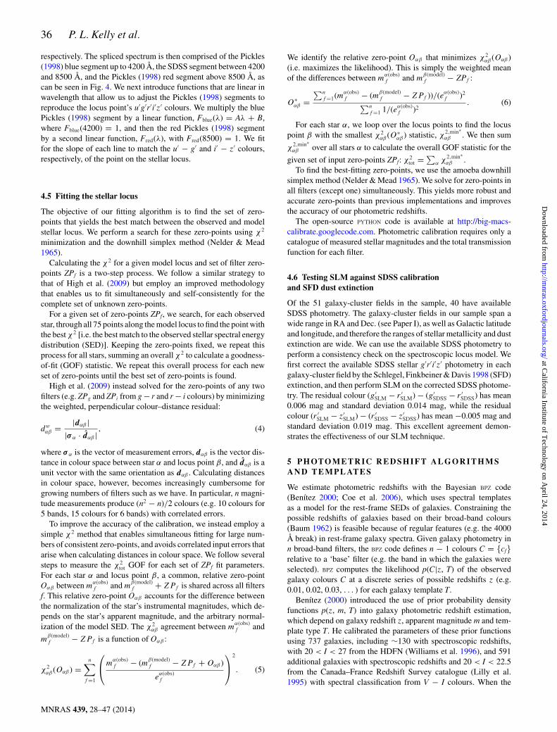
Figure 5. Best-fitting SED model for a sample galaxy’s broad-band magnitudes from the BPZ photometric redshift code (left-hand panel) and posterior redshiftprobability distribution (right-hand panel). In this example, the template with greatest posterior probability is the elliptical galaxy spectrum from Coleman, Wu& Weedman (1980), modified by Capak (2004). The red points in the left-hand panel show, in order of increasing central wavelength, the calibrated galaxymagnitude measured for the SuprimeCam BJ, VJ, RC, IC and z+ bands. The blue rectangles show the expected flux for the elliptical SED in these photometricbands. In the right-hand panel, the horizontal coordinate of the vertical red line is the spectroscopic redshift of this elliptical galaxy.
colours C are consistent with the SED templates at multiple red-shifts, the prior function can alleviate or break redshift degeneracies.Here, we use the Benıtez (2000) prior functions with a modest ad-justment that increases the probability at low redshift (z < 0.2; seeErben et al. 2009). The posterior redshift probability distribution is
p(z) ≡ p(z|C,m) ∝∑
T
p(C|z, T )p(z, m, T ). (7)
The posterior probability p(z) distribution is then smoothed,using the BPZ code, with a Gaussian that we specify to haveσ (z/(1 + z)) = 0.03.
5.1 Most probable redshift zp
The peak of the posterior redshift probability distribution p(z) is,by definition, the most probable redshift of the galaxy, zp (the BPZ
parameter BPZ_Z_B). We use BPZ to compute, from the estimatedp(z) distribution, the probability that the galaxy redshift is within±0.1(1+zp) of zp,
ODDS =∫ zp+0.1(1+zp)
zp−0.1(1+zp)p(z) dz. (8)
For example, the ODDS statistic for a Gaussian p(z) centred at zp
with standard deviation σ = 0.05(1 + zp) would be 0.95.
5.2 Template set
The performance of the BPZ code depends on the template library.For this study, we use the template set assembled by Capak (2004),which comprises elliptical, Sbc, Scd and Im spectra from Colemanet al. (1980) and two starburst templates from Kinney et al. (1996).Capak (2004) adjusted these templates both to increase agreementbetween spectroscopically determined redshifts and the BPZ mostprobable redshift zp and to match the colours of galaxies fainterthan the limiting magnitudes of spectroscopic samples.
The Capak (2004) templates are ordered by type (see list above),and, before fitting, we generate additional templates by interpolatingeight times between adjacent templates in this ordered list (i.e.INTER = 8).
Fig. 5 shows an example photometric redshift fit to a galaxywith BJVJRCICz+ magnitudes. We show the best-fitting templateand measured galaxy magnitudes, as well as the p(z) distributionand spectroscopic redshift value.
6 G A L A X Y S E D E X T R A P O L AT I O N TO FI N D u∗
A N D BJ ZERO-POI NTS
The photometric calibration of very blue filters, particularly u∗,from SLM is more challenging than for redder bands. Absorptionby metals at near-UV and blue-optical wavelengths causes the u∗
and BJ magnitudes of main-sequence stars to depend more stronglyon the chemical abundances in the stellar atmospheres than VJ, RC,IC and z+ magnitudes (see Section 4.2). Consequently, the stellarlocus shows more variation across the sky in the u∗ and BJ bandsthan in redder bandpasses.
We have therefore developed a technique to adjust Megaprime u∗-band and SuprimeCam BJ-band zero-points after SLM calibration.We use the BPZ photometric redshift code to calculate for eachgalaxy the expected u∗ and BJ magnitudes for each galaxy giventhe calibrated photometry at redder observer-frame wavelengths(e.g. VJ, RC, IC and z+), based on the best-fitting SED templatemodel (e.g. elliptical, Sbc) and redshift. Our method employs atraining set of 10 000 galaxies, drawn randomly from the galaxieswhose u∗ and BJ magnitudes have uncertainties less than 0.05 mag.We modify the photometry catalogue so that BJ magnitudes areassigned an uncertainty of 0.2 and every u+ magnitude is assignedan uncertainty of 90 mag (effectively removing any constraint fromu+ magnitudes).
MNRAS 439, 28–47 (2014)
at California Institute of T
echnology on April 24, 2014
http://mnras.oxfordjournals.org/
Dow
nloaded from
38 P. L. Kelly et al.
The zero-point corrections for the u∗ and BJ bands are estimatedas the median difference μ1/2 between the predicted and measuredmagnitudes for galaxies,
ZPnew − ZPold = μ1/2
(mBPZ
gal − mexpgal
), (9)
although the peak as opposed to median difference could possiblyyield improved accuracy. After calculating photometric redshiftsfor the training set of galaxies, we then reject any galaxy with BPZ
ODDS parameter less than 0.95 and most probable photometricredshift smaller than zp = 0.4 so that the 4000 Å break does notfall near the u∗ or BJ bandpasses. These criteria yield a sample of∼1000 training galaxies. We apply this technique to fields for whichwe have u∗ or BJ observations in addition to observations in at leastfour other bandpasses.
The zero-points we estimate with this technique will of coursedepend on the accuracy of the BPZ template set used to computethe expected u∗ and BJ magnitudes. This procedure generally yieldssmall ∼0.01 mag adjustments to the BJ-band zero-point calibratedthrough SLM. We do not use available u∗-band photometry formeasuring cluster masses (Paper III).
7 PH OTO M E T R I C C A L I B R AT I O N T E S T S
We demonstrate the reliability of the SLM zero-point calibration,as well as the performance of the redshift estimation, by comparingour estimates for the most probable photometric redshift zp andthe posterior probability distribution p(z) to redshifts derived fromspectra in both our galaxy-cluster fields and the COSMOS (Scovilleet al. 2007) field, as well as accurate photometric redshifts from 30-band photometry of COSMOS galaxies (COSMOS-30; Capak et al.2007; Ilbert et al. 2009).
7.1 Spectroscopic redshift comparisons in the cluster fields
7.1.1 Galaxy samples in cluster fields
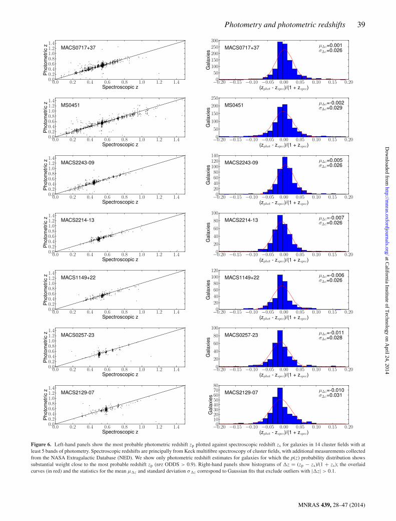
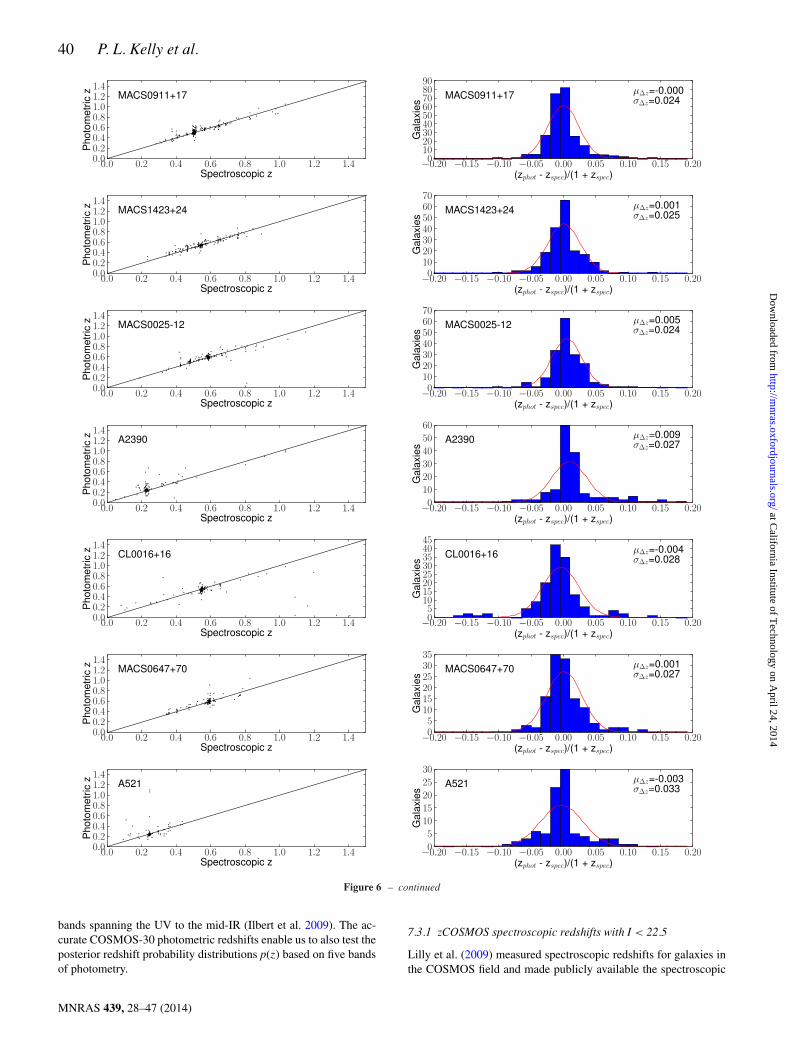
We have measured, or compiled from the NED,3 spectroscopicredshifts for 5007 galaxies in 27 cluster fields with five bands ofphotometry. We acquired spectra for galaxies in our cluster fields(e.g. Barrett 2006; Ma et al. 2008) with the Deep Imaging Multi-Object Spectrograph on the Keck-II telescope, the Low ResolutionImage Spectrometer (LRIS) on Keck-I, the Gemini Multi-ObjectSpectrographs on the Gemini telescope and the Visible Multi-ObjectSpectrograph on the Very Large Telescope (VLT). Of the 5007galaxies, 4735 (95 per cent) have BPZ ODDS > 0.9. In Fig. 6, we plotthe most probable photometric redshift zp versus the spectroscopicredshift zs for these galaxies with BPZ ODDS > 0.9 in the 14 clusterfields with the largest numbers of available spectroscopic redshifts.The photometric redshifts zp for each of these 14 fields have typicalaccuracy of σ ((zp − zs)/(1 + zs)) � 0.03 and bias (zp − zs)/(1 + zs)� 0.01, with |(zp − zs)/(1 + zs)| > 0.1 outliers excluded.
7.1.2 Combined sample of galaxies in cluster fields
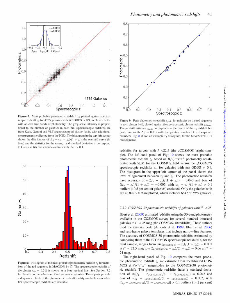
Fig. 7 compares the most probable photometric redshift zp to thespectroscopic redshift zs for the combined sample of galaxies withspectroscopic redshifts and BPZ ODDS > 0.9, across all clusterfields. The photometric redshifts have accuracy of σ ((zp − zs)/(1 + zs)) = 0.036 and bias of 〈(zp − zs)/(1 + zs)〉 = −0.001,
3 http://ned.ipac.caltech.edu/
with |zp − zs|/(1 + zs) > 0.1 outliers (8.2 per cent of galaxies)excluded.
The σ ((zp − zs)/(1 + zs)) = 0.036 distribution is tighter than theσ ((zp − zs)/(1 + zs)) ≈ 0.05 that might be expected for galaxieswith BPZ ODDS ≈ 0.95 (as defined in Section 5.1). A discrepancy,here as well as in comparisons that follow, can reasonably be at-tributed to the fact that the BPZ p(z) distribution is smoothed with aσ (z/(1 + z)) = 0.03 normal distribution before the ODDS parame-ter is calculated, and the fact that we reject |(zp − zs)/(1 + zs)| > 0.1outliers when we compute σ ((zp − zs)/(1 + zs)).
7.2 Photometric redshifts of galaxies on the red sequence
Using plots of galaxy colour versus magnitude for each cluster field(e.g. VJ − RC versus VJ), we find the best-fitting slope, interceptand width of the distributions of red sequence galaxies for eachcluster. We use these parameters to identify the galaxies along thered sequence (see Paper III for details). These samples may includeforeground and background galaxy populations that happen to havethe same colours and magnitudes as the red sequence – a contami-nation that becomes increasingly significant at fainter magnitudes.Fig. 8 shows the histogram of most probable photometric redshiftszp with BPZ ODDS > 0.90, for galaxies along the MACS0911+17red sequence.
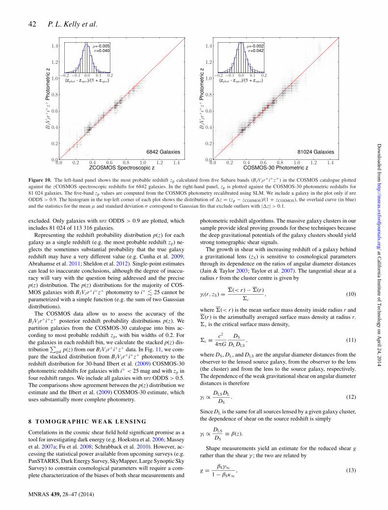
For cluster fields imaged through five or more filters (e.g.BJVJRCICz+), we plot in Fig. 9 the peak redshift in the histogramof most probable redshifts, zpeak, against the galaxy-cluster spec-troscopic redshift zcluster. While we have not otherwise made useof available near-UV photometry when computing photometricredshifts, we include CFHT MegaPrime u∗ photometry to esti-mate zpeak for the lowest redshift cluster in the sample, Abell 383,since near-UV photometry, combined with blue optical photome-try, bracket the 4000 Å break of z < 0.2 galaxies. The dispersionof zpeak is σ ((zpeak − zcluster)/(1 + zcluster)) = 0.011 and the biasis 〈(zpeak − zcluster)/(1 + zcluster)〉 = −0.005. The histogram binshave z = 0.01 width, which places a lower limit on the accuracyof the cluster redshift estimates. A more accurate estimate of thepeak cluster redshift could be obtained by applying, for example, aweighted Gaussian-kernel density estimator to interpolate betweenadjacent bins and by estimating photometric redshifts with greaterprecision than z = 0.01.
7.3 Galaxies in the COSMOS survey
Accurate redshifts based on 30-band photometry (Capak et al. 2007;Ilbert et al. 2009) are available for galaxies to i+ ≈ 25 mag in a2 deg2 field imaged for the COSMOS (Scoville et al. 2007). Spec-troscopic redshifts are also available for a sample of COSMOSgalaxies with I < 22.5 mag (zCOSMOS; Lilly et al. 2009). The pho-tometry of the COSMOS field includes SuprimeCam BJVJr+i+z+
magnitudes, which we use to estimate photometric redshifts in anidentical manner as for the photometry of the galaxy-cluster fields,after recalibrating their zero-points.
The magnitude limit of i+ ≈ 25 for the COSMOS catalogue iscomparable to that of our Subaru and CFHT galaxy-cluster imaging,and beyond the completeness limit of today’s spectroscopic sam-ples. To test the five-filter photometric redshift estimates, we applyto the COSMOS-30 photometry catalogue the same SLM and pho-tometric redshift estimation procedure as we do for the cluster fields.We compare our most probable BJVJr+i+z+ photometric redshiftszp to zCOSMOS spectroscopic redshifts and COSMOS-30 photo-metric redshifts estimated from 30 broad, intermediate and narrow
MNRAS 439, 28–47 (2014)
at California Institute of T
echnology on April 24, 2014
http://mnras.oxfordjournals.org/
Dow
nloaded from
Photometry and photometric redshifts 39
Figure 6. Left-hand panels show the most probable photometric redshift zp plotted against spectroscopic redshift zs for galaxies in 14 cluster fields with atleast 5 bands of photometry. Spectroscopic redshifts are principally from Keck multifibre spectroscopy of cluster fields, with additional measurements collectedfrom the NASA Extragalactic Database (NED). We show only photometric redshift estimates for galaxies for which the p(z) probability distribution showssubstantial weight close to the most probable redshift zp (BPZ ODDS > 0.9). Right-hand panels show histograms of z = (zp − zs)/(1 + zs); the overlaidcurves (in red) and the statistics for the mean μz and standard deviation σz correspond to Gaussian fits that exclude outliers with |z| > 0.1.
MNRAS 439, 28–47 (2014)
at California Institute of T
echnology on April 24, 2014
http://mnras.oxfordjournals.org/
Dow
nloaded from
40 P. L. Kelly et al.
Figure 6 – continued
bands spanning the UV to the mid-IR (Ilbert et al. 2009). The ac-curate COSMOS-30 photometric redshifts enable us to also test theposterior redshift probability distributions p(z) based on five bandsof photometry.
7.3.1 zCOSMOS spectroscopic redshifts with I < 22.5
Lilly et al. (2009) measured spectroscopic redshifts for galaxies inthe COSMOS field and made publicly available the spectroscopic
MNRAS 439, 28–47 (2014)
at California Institute of T
echnology on April 24, 2014
http://mnras.oxfordjournals.org/
Dow
nloaded from
Photometry and photometric redshifts 41
Figure 7. Most probable photometric redshift zp plotted against spectro-scopic redshift zs for 4735 galaxies with BPZ ODDS > 0.9, in cluster fieldswith at least five bands of photometry. The grey-scale intensity is propor-tional to the number of galaxies in each bin. Spectroscopic redshifts arefrom Keck, Gemini and VLT spectroscopy of cluster fields, with additionalmeasurements collected from the NED. The histogram in the top-left cornershows the distribution of z = (zp − zs)/(1 + zs); the overlaid curve (inblue) and the statistics for the mean μ and standard deviation σ correspondto Gaussian fits that exclude outliers with |z| > 0.1.
Figure 8. Histogram of the most probable photometric redshift zp for mem-bers of the red sequence in MACS0911+17. The spectroscopic redshift ofthe cluster (zs = 0.51) is shown as a blue vertical line. See Section 7.2for details on the selection of red sequence galaxies. These plots providea diagnostic check of the photometric redshift quality available even whenfew spectroscopic redshifts are available.
Figure 9. Peak photometric redshift zpeak, for galaxies on the red sequencein each cluster field, plotted against the spectroscopic cluster redshift zcluster.The redshift estimate zpeak corresponds to the centre of the zp redshift bin(with bin width z = 0.01) with the greatest number of red sequencemembers. Fig. 8 shows an example zp histogram, for the MACS 0911+17red sequence.
redshifts for targets with I <22.5 (the zCOSMOS bright sam-ple). The left-hand panel of Fig. 10 shows the most probablephotometric redshift zp based on BJVJr+i+z+ photometry recali-brated with SLM for the COSMOS field versus the zCOSMOSspectroscopic redshifts zs, for galaxies with BPZ ODDS > 0.9.The histogram in the upper-left corner of the panel shows thelevel of agreement between zp and zs. The photometric redshiftshave accuracy of σ ((zp − zs)/(1 + zs)) = 0.040 and bias of〈(zp − zs)/(1 + zs)〉 = −0.005, with |zp − zs|/(1 + zs) > 0.1outliers (10.5 per cent of galaxies) excluded. Only the galaxies withBPZ ODDS > 0.9 are plotted, which includes 6842 of 7959 galaxies.
7.3.2 COSMOS-30 photometric redshifts of galaxies with i+ < 25
Ilbert et al. (2009) estimated redshifts using the 30-band photometryavailable in the COSMOS survey for several hundred thousandgalaxies to i+ < 25 mag (the COSMOS-30 redshifts). These authorsused the LEPHARE code (Arnouts et al. 1999; Ilbert et al. 2006)and rest-frame galaxy templates that include narrow-line features.The accuracy of COSMOS-30 photometric redshifts, estimated bycomparing them to the zCOSMOS spectroscopic redshifts zs for thefaint sample, ranges from σ ((zCOSMOS-30 − zs)/(1 + zs)) = 0.007at i+ < 22.5 mag to σ ((zCOSMOS-30 − zs)/(1 + zs)) = 0.06 at i+ ≈24 mag.
The right-hand panel of Fig. 10 compares the most proba-ble photometric redshift zp we estimate from recalibrated COS-MOS BJVJr+i+z+ magnitudes to the COSMOS-30 photomet-ric redshift. The photometric redshifts have a standard devia-tion of σ ((zp − zCOSMOS-30)/(1 + zCOSMOS-30)) = 0.042 andbias of 〈(zp − zCOSMOS-30)/(1 + zCOSMOS-30)〉 = 0.002, with|(zp − zCOSMOS-30)/(1 + zCOSMOS-30)| > 0.1 outliers (14.2 per cent)
MNRAS 439, 28–47 (2014)
at California Institute of T
echnology on April 24, 2014
http://mnras.oxfordjournals.org/
Dow
nloaded from
42 P. L. Kelly et al.
Figure 10. The left-hand panel shows the most probable redshift zp calculated from five Subaru bands (BJVJr+i+z+) in the COSMOS catalogue plottedagainst the zCOSMOS spectroscopic redshifts for 6842 galaxies. In the right-hand panel, zp is plotted against the COSMOS-30 photometric redshifts for81 024 galaxies. The five-band zp values are computed from the COSMOS photometry recalibrated using SLM. We include a galaxy in the plot only if BPZ
ODDS > 0.9. The histogram in the top-left corner of each plot shows the distribution of z = (zp − zCOSMOS)/(1 + zCOSMOS), the overlaid curve (in blue)and the statistics for the mean μ and standard deviation σ correspond to Gaussian fits that exclude outliers with |z| > 0.1.
excluded. Only galaxies with BPZ ODDS > 0.9 are plotted, whichincludes 81 024 of 113 316 galaxies.
Representing the redshift probability distribution p(z) for eachgalaxy as a single redshift (e.g. the most probable redshift zp) ne-glects the sometimes substantial probability that the true galaxyredshift may have a very different value (e.g. Cunha et al. 2009;Abrahamse et al. 2011; Sheldon et al. 2012). Single-point estimatescan lead to inaccurate conclusions, although the degree of inaccu-racy will vary with the question being addressed and the precisep(z) distribution. The p(z) distributions for the majority of COS-MOS galaxies with BJVJr+i+z+ photometry to i+ � 25 cannot beparametrized with a simple function (e.g. the sum of two Gaussiandistributions).
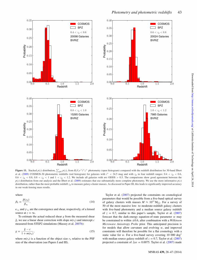
The COSMOS data allow us to assess the accuracy of theBJVJr+i+z+ posterior redshift probability distributions p(z). Wepartition galaxies from the COSMOS-30 catalogue into bins ac-cording to most probable redshift zp, with bin widths of 0.2. Forthe galaxies in each redshift bin, we calculate the stacked p(z) dis-tribution
∑gal p(z) from our BJVJr+i+z+ data. In Fig. 11, we com-
pare the stacked distribution from BJVJr+i+z+ photometry to theredshift distribution for 30-band Ilbert et al. (2009) COSMOS-30photometric redshifts for galaxies with i+ < 25 mag and with zp infour redshift ranges. We include all galaxies with BPZ ODDS > 0.5.The comparisons show agreement between the p(z) distribution weestimate and the Ilbert et al. (2009) COSMOS-30 estimate, whichuses substantially more complete photometry.
8 TO M O G R A P H I C W E A K L E N S I N G
Correlations in the cosmic shear field hold significant promise as atool for investigating dark energy (e.g. Hoekstra et al. 2006; Masseyet al. 2007a; Fu et al. 2008; Schrabback et al. 2010). However, ac-cessing the statistical power available from upcoming surveys (e.g.PanSTARRS, Dark Energy Survey, SkyMapper, Large Synoptic SkySurvey) to constrain cosmological parameters will require a com-plete characterization of the biases of both shear measurements and
photometric redshift algorithms. The massive galaxy clusters in oursample provide ideal proving grounds for these techniques becausethe deep gravitational potentials of the galaxy clusters should yieldstrong tomographic shear signals.
The growth in shear with increasing redshift of a galaxy behinda gravitational lens (zS) is sensitive to cosmological parametersthrough its dependence on the ratios of angular diameter distances(Jain & Taylor 2003; Taylor et al. 2007). The tangential shear at aradius r from the cluster centre is given by
γt(r, zS) = �(< r) − �(r)
�c
, (10)
where �(< r) is the mean surface mass density inside radius r and�(r) is the azimuthally averaged surface mass density at radius r.�c is the critical surface mass density,
�c ≡ c2
4πG
DS
DLDLS, (11)
where DS, DL, and DLS are the angular diameter distances from theobserver to the lensed source galaxy, from the observer to the lens(the cluster) and from the lens to the source galaxy, respectively.The dependence of the weak gravitational shear on angular diameterdistances is therefore
γt ∝ DLSDL
DS. (12)
Since DL is the same for all sources lensed by a given galaxy cluster,the dependence of shear on the source redshift is simply
γt ∝ DLS
DS≡ β(z).
Shape measurements yield an estimate for the reduced shear grather than the shear γ ; the two are related by
g = βSγ∞1 − βSκ∞
, (13)
MNRAS 439, 28–47 (2014)
at California Institute of T
echnology on April 24, 2014
http://mnras.oxfordjournals.org/
Dow
nloaded from
Photometry and photometric redshifts 43
Figure 11. Stacked p(z) distribution,∑
gal p(z), from BJVJr+i+z+ photometry (open histogram) compared with the redshift distribution for 30-band Ilbertet al. (2009) COSMOS-30 photometric redshifts (red histogram) for galaxies with i+ < 24.5 mag and with zp in four redshift ranges: 0.4 < zp < 0.6,0.6 < zp < 0.8, 0.8 < zp < 1 and 1 < zp < 1.2. We include all galaxies with BPZ ODDS > 0.5. The comparisons show good agreement between thep(z) distribution from our analysis and the Ilbert et al. (2009) estimates that use substantially more complete photometry. We use the more informative p(z)distribution, rather than the most probable redshift zp to measure galaxy-cluster masses. As discussed in Paper III, this leads to significantly improved accuracyin our weak-lensing mass results.
where
βS = β(zS)
β∞. (14)
κ∞ and γ ∞ are the convergence and shear, respectively, of a lensedsource at z = ∞.
To estimate the actual reduced shear g from the measured shearg, we use a linear shear correction with slope m(rh) and intercept cmeasured from STEP2 simulations (Massey et al. 2007b):
g = g − c
1 + m(rh), (15)
where m(rh) is a function of the object size rh relative to the PSFsize of the observation (see Papers I and III).
Taylor et al. (2007) projected the constraints on cosmologicalparameters that would be possible from a five-band optical surveyof galaxy clusters with masses M ≈ 1015 M . For a survey of50 of the most massive low- to moderate-redshift galaxy clusterswith five-band photometry and a median source galaxy redshiftof z = 0.7, similar to this paper’s sample, Taylor et al. (2007)forecast that the dark-energy equation-of-state parameter w maybe constrained to within ±0.6, after combination with a WilkinsonMicrowave Anisotropy Probe prior. This anticipated precision isfor models that allow curvature and evolving w, and improvedconstraints will therefore be possible for a flat cosmology with astatic value for w. For a five-band survey covering 10 000 deg2
with median source galaxy redshift of z = 0.7, Taylor et al. (2007)projected a constraint of w = 0.0075. Taylor et al. (2007) made
MNRAS 439, 28–47 (2014)
at California Institute of T
echnology on April 24, 2014
http://mnras.oxfordjournals.org/
Dow
nloaded from
44 P. L. Kelly et al.
the assumption that the errors of photometric redshifts are Gaussianand that any magnitude- or size-dependent bias in ground-basedshear measurements can be controlled to z = 1.5.
In a number of pioneering efforts, an increase in shear signal hasbeen observed with distance of the source galaxies behind groupsor clusters. Wittman et al. (2001) plotted the measured shear againstphotometric redshift for the galaxies lensed by a massive cluster atz = 0.276 (see also Wittman et al. 2003). Kitching et al. (2007)combined a tomographic analysis of the A901/2 supercluster, witha cosmic-shear analysis of two randomly selected fields using pho-tometric redshifts estimated by the Classifying Objects by Medium-Band Observations (COMBO-17) project. Medezinski et al. (2011)showed that the shear signal increases with distance of sources be-hind the A370, ZwCl0024+17 and RXJ1347−11 galaxy clusters,based on colour cuts applied to three-filter Subaru imaging. Tayloret al. (2012) measured the redshift dependence of the weak-lensingshear behind groups in the COSMOS field using Hubble Space Tele-scope images for shape measurements and the Ilbert et al. (2009)30-band photometric redshifts.
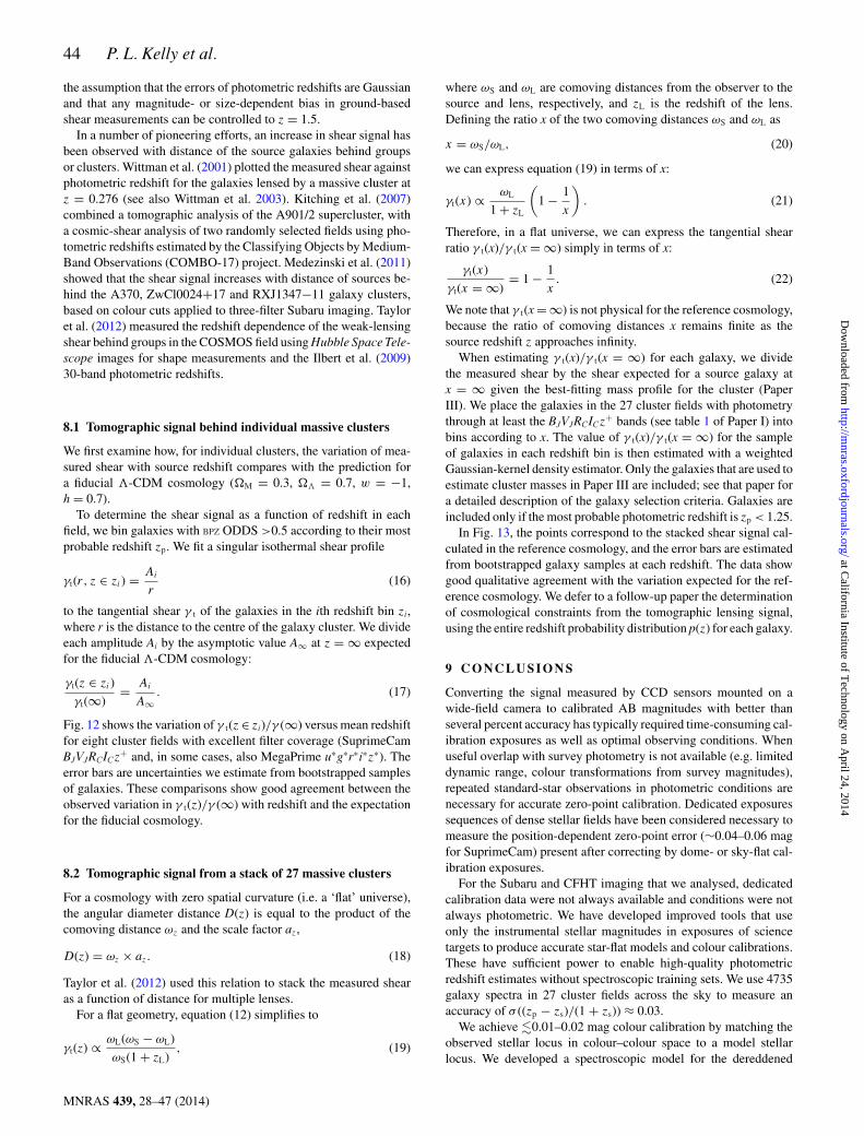
8.1 Tomographic signal behind individual massive clusters
We first examine how, for individual clusters, the variation of mea-sured shear with source redshift compares with the prediction fora fiducial �-CDM cosmology (�M = 0.3, �� = 0.7, w = −1,h = 0.7).
To determine the shear signal as a function of redshift in eachfield, we bin galaxies with BPZ ODDS >0.5 according to their mostprobable redshift zp. We fit a singular isothermal shear profile
γt(r, z ∈ zi) = Ai
r(16)
to the tangential shear γ t of the galaxies in the ith redshift bin zi,where r is the distance to the centre of the galaxy cluster. We divideeach amplitude Ai by the asymptotic value A∞ at z = ∞ expectedfor the fiducial �-CDM cosmology:
γt(z ∈ zi)
γt(∞)= Ai
A∞. (17)
Fig. 12 shows the variation of γ t(z ∈ zi)/γ (∞) versus mean redshiftfor eight cluster fields with excellent filter coverage (SuprimeCamBJVJRCICz+ and, in some cases, also MegaPrime u∗g∗r∗i∗z∗). Theerror bars are uncertainties we estimate from bootstrapped samplesof galaxies. These comparisons show good agreement between theobserved variation in γ t(z)/γ (∞) with redshift and the expectationfor the fiducial cosmology.
8.2 Tomographic signal from a stack of 27 massive clusters
For a cosmology with zero spatial curvature (i.e. a ‘flat’ universe),the angular diameter distance D(z) is equal to the product of thecomoving distance ωz and the scale factor az,
D(z) = ωz × az. (18)
Taylor et al. (2012) used this relation to stack the measured shearas a function of distance for multiple lenses.
For a flat geometry, equation (12) simplifies to
γt(z) ∝ ωL(ωS − ωL)
ωS(1 + zL), (19)
where ωS and ωL are comoving distances from the observer to thesource and lens, respectively, and zL is the redshift of the lens.Defining the ratio x of the two comoving distances ωS and ωL as
x = ωS/ωL, (20)
we can express equation (19) in terms of x:
γt(x) ∝ ωL
1 + zL
(1 − 1
x
). (21)
Therefore, in a flat universe, we can express the tangential shearratio γ t(x)/γ t(x = ∞) simply in terms of x:
γt(x)
γt(x = ∞)= 1 − 1
x. (22)
We note that γ t(x = ∞) is not physical for the reference cosmology,because the ratio of comoving distances x remains finite as thesource redshift z approaches infinity.
When estimating γ t(x)/γ t(x = ∞) for each galaxy, we dividethe measured shear by the shear expected for a source galaxy atx = ∞ given the best-fitting mass profile for the cluster (PaperIII). We place the galaxies in the 27 cluster fields with photometrythrough at least the BJVJRCICz+ bands (see table 1 of Paper I) intobins according to x. The value of γ t(x)/γ t(x = ∞) for the sampleof galaxies in each redshift bin is then estimated with a weightedGaussian-kernel density estimator. Only the galaxies that are used toestimate cluster masses in Paper III are included; see that paper fora detailed description of the galaxy selection criteria. Galaxies areincluded only if the most probable photometric redshift is zp < 1.25.
In Fig. 13, the points correspond to the stacked shear signal cal-culated in the reference cosmology, and the error bars are estimatedfrom bootstrapped galaxy samples at each redshift. The data showgood qualitative agreement with the variation expected for the ref-erence cosmology. We defer to a follow-up paper the determinationof cosmological constraints from the tomographic lensing signal,using the entire redshift probability distribution p(z) for each galaxy.
9 C O N C L U S I O N S
Converting the signal measured by CCD sensors mounted on awide-field camera to calibrated AB magnitudes with better thanseveral percent accuracy has typically required time-consuming cal-ibration exposures as well as optimal observing conditions. Whenuseful overlap with survey photometry is not available (e.g. limiteddynamic range, colour transformations from survey magnitudes),repeated standard-star observations in photometric conditions arenecessary for accurate zero-point calibration. Dedicated exposuressequences of dense stellar fields have been considered necessary tomeasure the position-dependent zero-point error (∼0.04–0.06 magfor SuprimeCam) present after correcting by dome- or sky-flat cal-ibration exposures.
For the Subaru and CFHT imaging that we analysed, dedicatedcalibration data were not always available and conditions were notalways photometric. We have developed improved tools that useonly the instrumental stellar magnitudes in exposures of sciencetargets to produce accurate star-flat models and colour calibrations.These have sufficient power to enable high-quality photometricredshift estimates without spectroscopic training sets. We use 4735galaxy spectra in 27 cluster fields across the sky to measure anaccuracy of σ ((zp − zs)/(1 + zs)) ≈ 0.03.
We achieve �0.01–0.02 mag colour calibration by matching theobserved stellar locus in colour–colour space to a model stellarlocus. We developed a spectroscopic model for the dereddened
MNRAS 439, 28–47 (2014)
at California Institute of T
echnology on April 24, 2014
http://mnras.oxfordjournals.org/
Dow
nloaded from
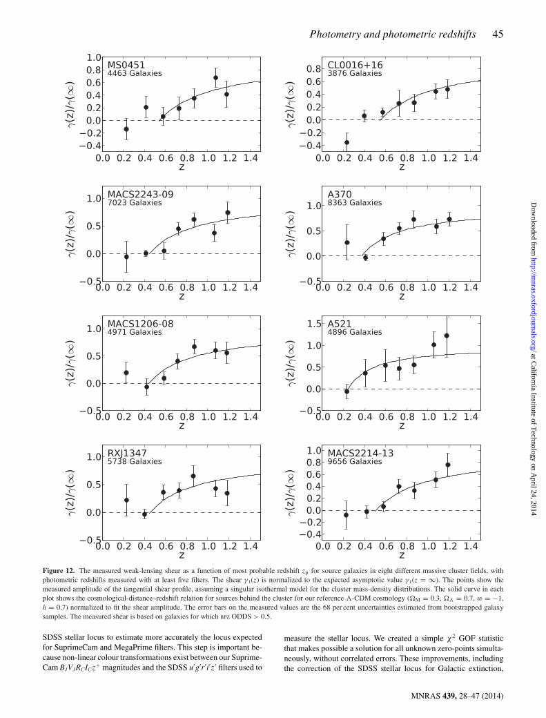
Photometry and photometric redshifts 45
Figure 12. The measured weak-lensing shear as a function of most probable redshift zp for source galaxies in eight different massive cluster fields, withphotometric redshifts measured with at least five filters. The shear γ t(z) is normalized to the expected asymptotic value γ t(z = ∞). The points show themeasured amplitude of the tangential shear profile, assuming a singular isothermal model for the cluster mass-density distributions. The solid curve in eachplot shows the cosmological-distance–redshift relation for sources behind the cluster for our reference �-CDM cosmology (�M = 0.3, �� = 0.7, w = −1,h = 0.7) normalized to fit the shear amplitude. The error bars on the measured values are the 68 per cent uncertainties estimated from bootstrapped galaxysamples. The measured shear is based on galaxies for which BPZ ODDS > 0.5.
SDSS stellar locus to estimate more accurately the locus expectedfor SuprimeCam and MegaPrime filters. This step is important be-cause non-linear colour transformations exist between our Suprime-Cam BJVJRCICz+ magnitudes and the SDSS u′g′r′i′z′ filters used to
measure the stellar locus. We created a simple χ2 GOF statisticthat makes possible a solution for all unknown zero-points simulta-neously, without correlated errors. These improvements, includingthe correction of the SDSS stellar locus for Galactic extinction,
MNRAS 439, 28–47 (2014)
at California Institute of T
echnology on April 24, 2014
http://mnras.oxfordjournals.org/
Dow
nloaded from
46 P. L. Kelly et al.
Figure 13. The stacked shear ratio for 27 clusters as a function of scaledcomoving distance. The horizontal axis is the ratio of comoving distancesfrom the observer to the source galaxy and to the lens. The vertical axisis the shear signal divided by that for a hypothetical (although physicallydisallowed) source at x = ∞ calculated for the fiducial cosmology and thebest-fitting cluster mass (from Paper III). The black curve is the predictedshear scaling 1 − 1/x for the reference cosmology. Points are the modes(maximum likelihood) measured from a Gaussian-kernel density estimator,and the error bars represent the 68 per cent confidence interval as estimatedfrom bootstrapped samples of galaxies in each bin.
were necessary to estimate robust and reliable photometric red-shifts from our Subaru and CFHT imaging. Interested readers mayfind the PYTHON code as well as a spectroscopic model for the locusat http://big-macs-calibrate.googlecode.com. Calibration requiresonly a catalogue of stellar magnitudes and the total transmissionfunction for each bandpass filter.
Summarizing the redshift posterior probability distribution p(z)for each galaxy as a single redshift (e.g. the most probable redshiftzp) disregards any probability that the true galaxy redshift may havea very different value (e.g. catastrophic outliers). The p(z) distri-bution contains more information than the most probable redshift,or other single-point estimates. We find good agreement betweenthe stacked
∑gal p(z) and the redshift distribution estimated from
30 COSMOS photometric bands by Ilbert et al. (2009). The p(z)distributions will provide a more powerful, less biased tool for sci-ence analysis than single-point estimates for ongoing and futuresurveys (e.g. PanSTARRS, Dark Energy Survey, SkyMapper, LargeSynoptic Sky Survey).
The extreme gravitational potentials of massive galaxy clustersare expected to yield a simple, strong growth in shear signal withincreasing distance of the source galaxy behind the cluster lens.The shape of the growth of shear behind a stack of 27 clusterswith increasing redshift shows agreement with a fiducial �-CDMcosmology. The average shear we measure for foreground galaxiesis consistent with zero.
The software we make available can produce state-of-the-art pho-tometric accuracy without dedicated observations or the need toestimate non-linear colour terms. Stellar colours will be a use-ful tool for checking the accuracy of zero-points obtained throughubercalibration of surveys (e.g. Ivezic et al. 2007; Padmanabhanet al. 2008; Schlafly et al. 2012) or close monitoring of atmospherictransparency (e.g. Burke et al. 2010; Blake & Shaw 2011).
AC K N OW L E D G E M E N T S
We thank F. William High, Jorg Dietrich and Hendrik Hildebrandtfor their expert advice and assistance on photometric calibrationand redshift estimation. We also appreciate helpful discussions withThomas Erben, C-J Ma, Daniel Coe and Carlos Cunha.
This work is supported in part by the US Department of Energyunder contract number DE-AC02-76SF00515. This work was alsosupported by the National Science Foundation under Grant nos.AST-0807458 and AST-1140019. MTA and PRB acknowledge thesupport of NSF grant PHY-0969487. AM acknowledges the sup-port of NSF grant AST-0838187. The authors acknowledge sup-port from programmes HST-AR-12654.01-A, HST-GO-12009.02-A and HST-GO-11100.02-A provided by NASA through a grantfrom the Space Telescope Science Institute, which is operated bythe Association of Universities for Research in Astronomy, Inc., un-der NASA contract NAS 5-26555. This work is also supported bythe National Aeronautics and Space Administration through Chan-dra Award Numbers TM1-12010X, GO0-11149X, GO9-0141X andGO8-9119X issued by the Chandra X-ray Observatory Center,which is operated by the Smithsonian Astrophysical Observatoryfor and on behalf of the National Aeronautics Space Administra-tion under contract NAS8-03060. DEA recognizes the support of aHewlett Foundation Stanford Graduate Fellowship.
Based in part on data collected at Subaru Telescope (Universityof Tokyo) and obtained from the SMOKA, which is operated bythe Astronomy Data Center, National Astronomical Observatory ofJapan. Based on observations obtained with MegaPrime/MegaCam,a joint project of CFHT and CEA/DAPNIA, at the CFHT, whichis operated by the National Research Council (NRC) of Canada,the Institute National des Sciences de l’Univers of the Centre Na-tional de la Recherche Scientifique of France and the Universityof Hawaii. This research used the facilities of the Canadian As-tronomy Data Centre operated by the National Research Councilof Canada with the support of the Canadian Space Agency. Thisresearch has made use of the VizieR catalogue access tool, CDS,Strasbourg, France. Funding for SDSS-III has been provided by theAlfred P. Sloan Foundation, the Participating Institutions, the Na-tional Science Foundation and the US Department of Energy Officeof Science. The SDSS-III website is http://www.sdss3.org/. Thisresearch has made use of the NASA/IPAC Extragalactic Database(NED), which is operated by the Jet Propulsion Laboratory, Caltech,under contract with NASA.
R E F E R E N C E S
Abrahamse A., Knox L., Schmidt S., Thorman P., Tyson J. A., Zhan H.,2011, ApJ, 734, 36
Aihara H. et al., 2011, ApJS, 193, 29Applegate D. E. et al., 2014, MNRAS, 439, 48Arnouts S., Cristiani S., Moscardini L., Matarrese S., Lucchin F., Fontana
A., Giallongo E., 1999, MNRAS, 310, 540Baba H. et al., 2002, Rep. Natl. Astron. Obs. Japan, 6, 23Barrett E., 2006, PhD thesis, Univ. Hawai’i at ManoaBaum W. A., 1962, in McVittie G. C., ed., Proc. IAU Symp. Vol. 15, Prob-
lems of Extra-Galactic Research. Macmillan, New York, p. 390Benıtez N., 2000, ApJ, 536, 571Bertin E., Arnouts S., 1996, A&AS, 117, 393Bertin E., Mellier Y., Radovich M., Missonnier G., Didelon P., Morin B.,
2002, in Bohlender D. A., Durand D., Handley T. H., eds, ASP Conf.Ser. Vol. 281, Astronomical Data Analysis Software and Systems XI.Astron. Soc. Pac., San Francisco, p. 228
Blake C. H., Shaw M. M., 2011, PASP, 123, 1302Burke D. L. et al., 2010, ApJ, 720, 811
MNRAS 439, 28–47 (2014)
at California Institute of T
echnology on April 24, 2014
http://mnras.oxfordjournals.org/
Dow
nloaded from
Photometry and photometric redshifts 47
Capak P. L., 2004, PhD thesis, Univ. HawaiiCapak P. et al., 2007, ApJS, 172, 99Coe D., Benıtez N., Sanchez S. F., Jee M., Bouwens R., Ford H., 2006, AJ,
132, 926Coleman G. D., Wu C.-C., Weedman D. W., 1980, ApJS, 43, 393Coupon J. et al., 2012, A&A, 542, A5Covey K. R. et al., 2007, AJ, 134, 2398Cunha C. E., Lima M., Oyaizu H., Frieman J., Lin H., 2009, MNRAS, 396,
2379Davis T. A., 2006, Fundamentals of Algorithms: Direct Methods for Sparse
Linear Systems. SIAM, Philadelphia, PADrimmel R., Spergel D. N., 2001, ApJ, 556, 181Ebeling H., Edge A. C., Henry J. P., 2001, ApJ, 553, 668Ebeling H., Barrett E., Donovan D., Ma C.-J., Edge A. C., van Speybroeck
L., 2007, ApJ, 661, L33Ebeling H., Edge A. C., Mantz A., Barrett E., Henry J. P., Ma C. J.,
van Speybroeck L., 2010, MNRAS, 407, 83Erben T. et al., 2005, Astron. Nachr., 326, 432Erben T. et al., 2009, A&A, 493, 1197Fu L. et al., 2008, A&A, 479, 9Gilbank D. G., Gladders M. D., Yee H. K. C., Hsieh B. C., 2011, AJ, 141,
94Kitching T. D., Heavens A. F., Taylor A. N., Brown M. L., Meisenheimer
K., Wolf C., Gray M. E., Bacon D. J., 2007, MNRAS, 376, 771High F. W., Stubbs C. W., Rest A., Stalder B., Challis P., 2009, AJ, 138, 110High F. W. et al., 2010, ApJ, 723, 1736Hoekstra H. et al., 2006, ApJ, 647, 116Ilbert O. et al., 2006, A&A, 457, 841Ilbert O. et al., 2009, ApJ, 690, 1236Ivezic Z. et al., 2004, Astron. Nachr., 325, 583Ivezic Z. et al., 2007, AJ, 134, 973Ivezic Z. et al., 2008, ApJ, 684, 287Jain B., Taylor A., 2003, Phys. Rev. Lett., 91, 141302Jones D. O., West A. A., Foster J. B., 2011, AJ, 142, 44Kalberla P. M. W., Kerp J., 2009, ARA&A, 47, 27Kinney A. L., Calzetti D., Bohlin R. C., McQuade K., Storchi-Bergmann
T., Schmitt H. R., 1996, ApJ, 467, 38Koch A., Odenkirchen M., Caldwell J. A. R., Grebel E. K., 2003, Astron.
Nachr. Suppl., 324, 95
Kron R. G., 1980, ApJS, 43, 305Lilly S. J., Le Fevre O., Crampton D., Hammer F., Tresse L., 1995, ApJ,
455, 50Lilly S. J. et al., 2009, ApJS, 184, 218LSST Science Collaborations et al., 2009, arXiv:e-printsMacDonald E. C. et al., 2004, MNRAS, 352, 1255Magnier E. A., Cuillandre J.-C., 2004, PASP, 116, 449Ma C.-J., Ebeling H., Donovan D., Barrett E., 2008, ApJ, 684, 160Manfroid J., Selman F., Jones H., 2001, The Messenger, 104, 16Marshall D. J., Robin A. C., Reyle C., Schultheis M., Picaud S., 2006, A&A,
453, 635Massey R. et al., 2007a, ApJS, 172, 239Massey R. et al., 2007b, MNRAS, 376, 13Medezinski E., Broadhurst T., Umetsu K., Benıtez N., Taylor A., 2011,
MNRAS, 414, 1840Nelder J. A., Mead R., 1965, Comput. J., 7, 308Padmanabhan N. et al., 2008, ApJ, 674, 1217Pickles A. J., 1998, PASP, 110, 863Regnault N. et al., 2009, A&A, 506, 999Schlafly E. F. et al., 2012, ApJ, 756, 158Schlegel D. J., Finkbeiner D. P., Davis M., 1998, ApJ, 500, 525Schrabback T. et al., 2010, A&A, 516, A63Scoville N. et al., 2007, ApJS, 172, 1Sheldon E. S., Cunha C., Mandelbaum R., Brinkmann J., Weaver B. A.,
2012, ApJS, 201, 32Taylor A. N., Kitching T. D., Bacon D. J., Heavens A. F., 2007, MNRAS,
374, 1377Taylor J. E. et al., 2012, ApJ, 749, 127von der Linden A. et al., 2014, MNRAS, 439, 2West A. A. et al., 2011, AJ, 141, 97Williams R. E. et al., 1996, AJ, 112, 1335Wittman D., Tyson J. A., Margoniner V. E., Cohen J. G., Dell’Antonio I. P.,
2001, ApJ, 557, L89Wittman D., Margoniner V. E., Tyson J. A., Cohen J. G., Becker A. C.,
Dell’Antonio I. P., 2003, ApJ, 597, 218Wittman D., Ryan R., Thorman P., 2012, MNRAS, 421, 2251
This paper has been typeset from a TEX/LATEX file prepared by the author.
MNRAS 439, 28–47 (2014)
at California Institute of T
echnology on April 24, 2014
http://mnras.oxfordjournals.org/
Dow
nloaded from