CAFEE Center for Alternative Fuels, Engines and Emissions

West Virginia University

Final Report

Fuel consumption and emissions testing of a best-in-class tractor-trailer in the US

Submitted to: International Council on Clean Transportation (ICCT)

Prepared by: Arvind Thiruvengadam (Joint-Principal Investigator)

Marc C. Besch (Joint-Principal Investigator) Berk Demirgök (Co-Principal Investigator)

Dan Carder (Co-Principal Investigator) Cem Baki

Center for Alternative Fuels, Engines & Emissions Dept. of Mechanical & Aerospace Engineering

West Virginia University Morgantown WV 26506-6106

May 15, 2018

Acknowledgment

Page | 1

ACKNOWLEDGMENT WVU would like to thank Felipe Rodriguez and Oscar Delgado from the International Council

on Clean Transportation for their valuable and vital input during the course of this project as well

as providing their expertise and support in regards to the coastdown procedure and understanding

the workings of the VECTO simulation tool.

WVU thanks ICCT for providing the funding for this research project.

Table of Contents

Page | 1

TABLE OF CONTENTS Acknowledgment ........................................................................................................................ 1

Table of Contents ....................................................................................................................... 1

List of Tables.............................................................................................................................. 1

LIST OF FIGURES .................................................................................................................... 1

1 Introduction ........................................................................................................................ 1

2 Methodology....................................................................................................................... 1

2.1 Selection of vehicle ...................................................................................................... 1

2.2 Air drag measurements ................................................................................................. 2

2.2.1 Constant Speed Test .............................................................................................. 3

2.2.2 Coastdown Test ..................................................................................................... 6

2.3 Chassis dynamometer testing ...................................................................................... 12

2.3.1 Test Fuel Specifications ....................................................................................... 12

2.3.2 Test Cycles .......................................................................................................... 12

2.3.3 Chassis Dynamometer Measurements .................................................................. 15

2.3.4 Test Procedures ................................................................................................... 16

2.4 Data evaluation ........................................................................................................... 18

3 Results and Discussion........................................................................................................ 1

3.1 Average Wheel Work ................................................................................................... 1

3.2 Fuel Consumption ........................................................................................................ 2

3.3 Steady-state Engine Mapping Results ........................................................................... 3

4 References .......................................................................................................................... 1

List of Tables

Page | 1

LIST OF TABLES Table 2.1: Specifications of the tractor. ....................................................................................... 2

Table 2.2: Test trailer specifications............................................................................................ 2

Table 2.3: Weather conditions during CST. ................................................................................ 3

Table 2.4: Measurement systems and instruments. ...................................................................... 4

Table 2.5: Specifications of high resolution wheel torque meter TWHR2000. ............................. 4

Table 2.6: Results for the constant speed testing methodology .................................................... 6

Table 2.7: Vehicle speed ranges applied during coastdown testing. ............................................. 7

Table 2.8: Weather conditions during coastdown testing. ............................................................ 7

Table 2.9: Results of tire rolling resistance test. .......................................................................... 8

Table 2.10: Results of the coastdown tests. ................................................................................. 8

Table 2.11: Upper and lower limits for validation. ...................................................................... 9

Table 2.12: Comparison drag area results between constant speed and coastdown methods. ..... 10

Table 2.13: ULSD test fuel specifications. ................................................................................ 12

Table 2.14: Chassis dynamometer test cycle characteristics. ..................................................... 13

Table 2.15: Specifications of heavy-duty chassis dynamometer at ARB facility, Sacramento, CA. ................................................................................................................................................. 15

Table 2.16: Measurement systems and parameters [5]. .............................................................. 16

Table 2.17: Chassis dynamometer warm-up procedure. ............................................................ 17

Table 3.2: Selected steady-state test points. ................................................................................. 3

List of Figures

Page | 1

LIST OF FIGURES Figure 2.1: High resolution wheel torque meters installed on test vehicle. ................................... 5

Figure 2.2: Yaw angle correction function over an interval of yaw angle = 0 to 1º; ‘orange square’ indicating actual coastdown results from this study. .................................................................. 10

Figure 2.3: Drag area vs. yaw angle for different measurement methods. .................................. 11

Figure 2.4: Chassis dynamometer test cycles: a) VECTO long haul, b) VECTO regional delivery, c) GEM 55 with grade, and d) GEM ARB transient cycle. ........................................................ 14

Figure 2.5: Losses estimated from chassis dynamometer calibration procedure. ........................ 18

Figure 3.1: Comparison of distance-specific positive wheel work in [kWh/km] between experimental results and simulations for the different chassis dynamometer cycles. .................... 1

Figure 3.2: Comparison of distance-specific fuel consumption between gravimetric and ECU-broadcasted calculation methods in [L/100km] for the different chassis dynamometer cycles. .... 2

Figure 3.3: Comparison of work-specific fuel consumption between gravimetric and ECU-broadcasted calculation methods in [g/kWh] for the different chassis dynamometer cycles. ........ 2

Figure 3.4 Comparison of CO2 emissions in [g/t-km] between the different chassis dynamometer cycles. ........................................................................................................................................ 3

Figure 3.5: Steady-state brake-specific fuel consumption in [g/kWh] calculated through gravimetric fuel measurement and ECU derived engine work. .................................................... 4

Figure 3.6: Steady-state brake-specific fuel consumption in [g/kWh] calculated through ECU-broadcasted fuel measurement and ECU derived engine work. ................................................... 5

Figure 3.7: Steady-state engine thermal brake efficiency [%] calculated through gravimetric fuel measurement and ECU derived engine work. .............................................................................. 6

Methodology

Page | 1

1 INTRODUCTION The primary objective of this study was to conduct aerodynamic testing on a closed test track

along with chassis dynamometer testing of a US heavy-duty Diesel (HDD), Class 8 tractor to assess

the fuel consumption over prescribed driving cycles. The air drag was measured following the

coastdown (CD) procedure specified in US regulation [1], as well as the constant speed tests (CST)

defined in the European regulation [2]. The results were used to determine speed-based road load

forces onto the vehicle for subsequent chassis dynamometer testing.

2 METHODOLOGY

This chapter will discuss the selection of the test vehicle and its specifications in the first

Section 2.1, followed by a discussion of the constant speed test and coastdown methodology for

air drag evaluation in Sections 2.2.1 and 2.2.2, respectively. Finally, Section 2.3 will present the

vehicle chassis dynamometer testing procedure employed during the herein presented study.

2.1 Selection of vehicle The tractor and trailer combination was selected to represent the ‘best-available’ technology

in 2015, as evaluated with the support of the manufacturer, and which exhibits significant market

presence in the United States (US). The Center for Alternative Fuels, Engines and Emissions

(CAFEE) was able to recruit a suitable heavy-duty Diesel Class 8 tractor directly from the

respective OEM. In conjunction with the tractor, a conventional US trailer was selected that was

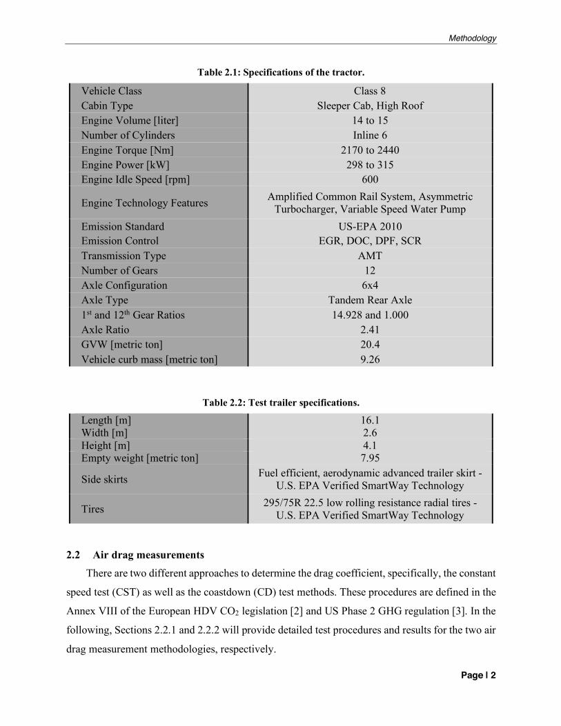
outfitted with side-skirts for aerodynamic enhancement. Table 2.1 provides the specifications of

the tractor selected for this study. The engine specifications are provided in ranges in order to

conceal the model and make of the truck being tested.

The trailer used during the air drag measurement was equipped with 2 axles, with spring rides,

and a composite plate van. All specifications of the test trailer were compliant with the provisions

stipulated in the US regulation for testing of heavy-duty motor vehicles [3] as listed in Table 2.2.

Methodology

Page | 2

Table 2.1: Specifications of the tractor.

Vehicle Class Class 8 Cabin Type Sleeper Cab, High Roof Engine Volume [liter] 14 to 15 Number of Cylinders Inline 6 Engine Torque [Nm] 2170 to 2440 Engine Power [kW] 298 to 315 Engine Idle Speed [rpm] 600

Engine Technology Features Amplified Common Rail System, Asymmetric Turbocharger, Variable Speed Water Pump

Emission Standard US-EPA 2010 Emission Control EGR, DOC, DPF, SCR Transmission Type AMT Number of Gears 12 Axle Configuration 6x4 Axle Type Tandem Rear Axle 1st and 12th Gear Ratios 14.928 and 1.000 Axle Ratio 2.41 GVW [metric ton] 20.4 Vehicle curb mass [metric ton] 9.26

Table 2.2: Test trailer specifications.

Length [m] 16.1 Width [m] 2.6 Height [m] 4.1 Empty weight [metric ton] 7.95

Side skirts Fuel efficient, aerodynamic advanced trailer skirt - U.S. EPA Verified SmartWay Technology

Tires 295/75R 22.5 low rolling resistance radial tires - U.S. EPA Verified SmartWay Technology

2.2 Air drag measurements

There are two different approaches to determine the drag coefficient, specifically, the constant

speed test (CST) as well as the coastdown (CD) test methods. These procedures are defined in the

Annex VIII of the European HDV CO2 legislation [2] and US Phase 2 GHG regulation [3]. In the

following, Sections 2.2.1 and 2.2.2 will provide detailed test procedures and results for the two air

drag measurement methodologies, respectively.

Methodology

Page | 3

Air drag measurements were completed at Michelin’s Laurens Proving Ground facility in

Laurens, SC, USA. Track 9 was the most suitable track for constant speed and coastdown tests at

this facility and is characterized by a 1463 meters straight section, with near perfect flatness, and

a track width of 12 to 20 meters. The straight center section of the track was connected to two

loops at each end allowing for the vehicle to return and accelerate back to the measurement section

without coming to a halt. The surface texture of Track 9 was smooth at a macro scale and rough at

a micro scale.

2.2.1 Constant Speed Test Following the provisions stipulated in the EU for the aerodynamic testing of heavy-duty

vehicles [2], WVU performed a constant speed test to determine the total forces onto the vehicle

at two different speeds. The direct measurement of the road-load forces is necessary for the

calculation of aerodynamic drag and tire rolling resistance in the CST method. For this purpose,

an appropriate wheel torque meter was used to measure the wheel forces. Since the test vehicle

has two driven axles (i.e. 6x4 axle configuration), both axles were equipped with wheel torque

meters. The wheel torque meter was attached to the drive axles and the vehicle was operated at

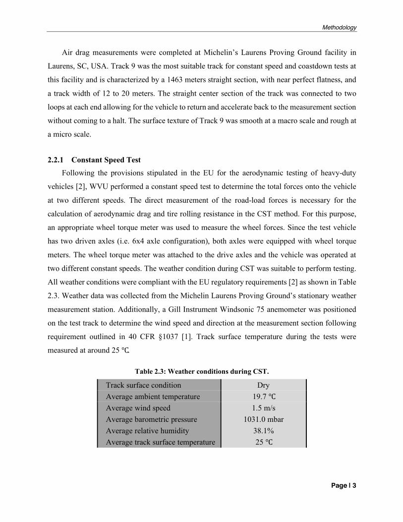
two different constant speeds. The weather condition during CST was suitable to perform testing.

All weather conditions were compliant with the EU regulatory requirements [2] as shown in Table

2.3. Weather data was collected from the Michelin Laurens Proving Ground’s stationary weather

measurement station. Additionally, a Gill Instrument Windsonic 75 anemometer was positioned

on the test track to determine the wind speed and direction at the measurement section following

requirement outlined in 40 CFR §1037 [1]. Track surface temperature during the tests were

measured at around 25 ℃.

Table 2.3: Weather conditions during CST.

Track surface condition Dry Average ambient temperature 19.7 ℃ Average wind speed 1.5 m/s Average barometric pressure 1031.0 mbar Average relative humidity 38.1% Average track surface temperature 25 ℃

Methodology

Page | 4

A second Gill Instrument Windsonic 75 anemometer was placed at a height of 1.5 meters

above the top surface of the trailer to measure air speeds as the vehicle was driving down the test

section. A K-Type thermocouple was placed on the pole of anemometer in order to determine the

ambient air temperature. Proving ground surface temperatures were periodically measured

manually with an infrared temperature sensor during the tests to ensure that the surface temperature

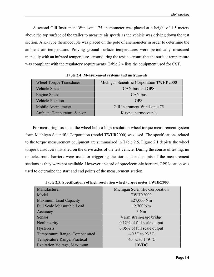
was compliant with the regulatory requirements. Table 2.4 lists the equipment used for CST.

Table 2.4: Measurement systems and instruments.

Wheel Torque Transducer Michigan Scientific Corporation TWHR2000 Vehicle Speed CAN bus and GPS Engine Speed CAN bus Vehicle Position GPS Mobile Anemometer Gill Instrument Windsonic 75 Ambient Temperature Sensor K-type thermocouple

For measuring torque at the wheel hubs a high resolution wheel torque measurement system

form Michigan Scientific Corporation (model TWHR2000) was used. The specifications related

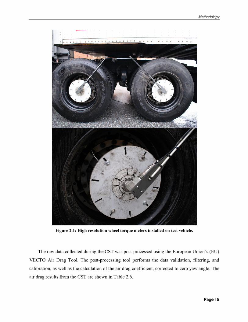
to the torque measurement equipment are summarized in Table 2.5. Figure 2.1 depicts the wheel

torque transducers installed on the drive axles of the test vehicle. During the course of testing, no

optoelectronic barriers were used for triggering the start and end points of the measurement

sections as they were not available. However, instead of optoelectronic barriers, GPS location was

used to determine the start and end points of the measurement section.

Table 2.5: Specifications of high resolution wheel torque meter TWHR2000.

Manufacturer Michigan Scientific Corporation Model TWHR2000 Maximum Load Capacity ±27,000 Nm Full Scale Measurable Load ±2,700 Nm Accuracy 3 Nm Sensor 4 arm strain-gage bridge Nonlinearity 0.12% of full scale output Hysteresis 0.05% of full scale output Temperature Range, Compensated -40 °C to 93 °C Temperature Range, Practical -40 °C to 149 °C Excitation Voltage, Maximum 10VDC

Methodology

Page | 5

Figure 2.1: High resolution wheel torque meters installed on test vehicle.

The raw data collected during the CST was post-processed using the European Union’s (EU)

VECTO Air Drag Tool. The post-processing tool performs the data validation, filtering, and

calibration, as well as the calculation of the air drag coefficient, corrected to zero yaw angle. The

air drag results from the CST are shown in Table 2.6.

Methodology

Page | 6

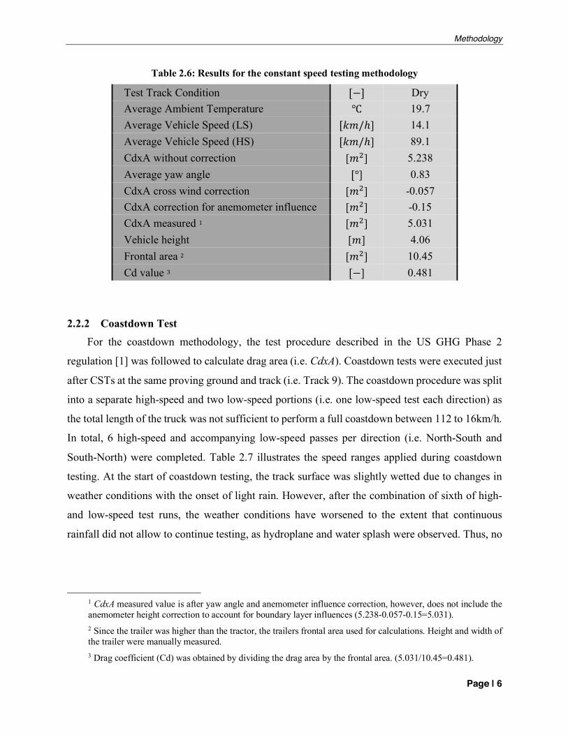
Table 2.6: Results for the constant speed testing methodology

Test Track Condition [−] Dry Average Ambient Temperature ℃ 19.7 Average Vehicle Speed (LS) [𝑘𝑚/ℎ] 14.1 Average Vehicle Speed (HS) [𝑘𝑚/ℎ] 89.1 CdxA without correction [𝑚)] 5.238 Average yaw angle [°] 0.83 CdxA cross wind correction [𝑚)] -0.057 CdxA correction for anemometer influence [𝑚)] -0.15 CdxA measured 1 [𝑚)] 5.031 Vehicle height [𝑚] 4.06 Frontal area 2 [𝑚)] 10.45 Cd value 3 [−] 0.481

2.2.2 Coastdown Test For the coastdown methodology, the test procedure described in the US GHG Phase 2

regulation [1] was followed to calculate drag area (i.e. CdxA). Coastdown tests were executed just

after CSTs at the same proving ground and track (i.e. Track 9). The coastdown procedure was split

into a separate high-speed and two low-speed portions (i.e. one low-speed test each direction) as

the total length of the truck was not sufficient to perform a full coastdown between 112 to 16km/h.

In total, 6 high-speed and accompanying low-speed passes per direction (i.e. North-South and

South-North) were completed. Table 2.7 illustrates the speed ranges applied during coastdown

testing. At the start of coastdown testing, the track surface was slightly wetted due to changes in

weather conditions with the onset of light rain. However, after the combination of sixth of high-

and low-speed test runs, the weather conditions have worsened to the extent that continuous

rainfall did not allow to continue testing, as hydroplane and water splash were observed. Thus, no

1 CdxA measured value is after yaw angle and anemometer influence correction, however, does not include the anemometer height correction to account for boundary layer influences (5.238-0.057-0.15=5.031). 2 Since the trailer was higher than the tractor, the trailers frontal area used for calculations. Height and width of the trailer were manually measured. 3 Drag coefficient (Cd) was obtained by dividing the drag area by the frontal area. (5.031/10.45=0.481).

Methodology

Page | 7

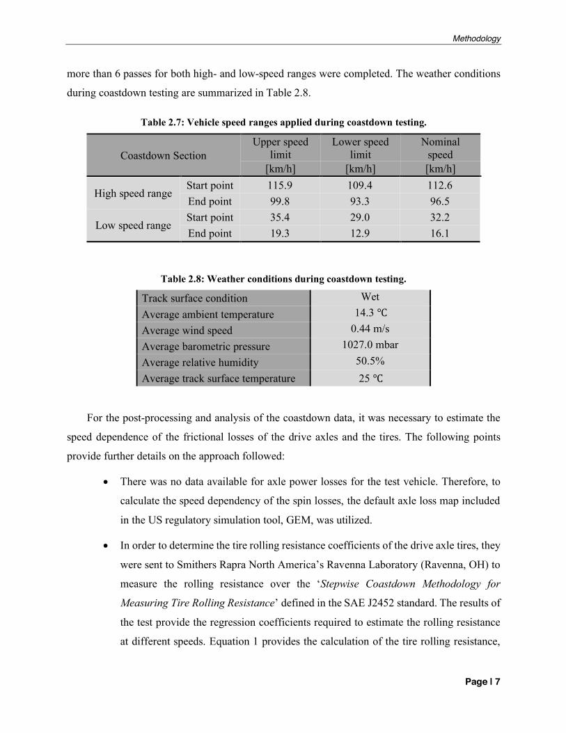
more than 6 passes for both high- and low-speed ranges were completed. The weather conditions

during coastdown testing are summarized in Table 2.8.

Table 2.7: Vehicle speed ranges applied during coastdown testing.

Coastdown Section Upper speed

limit Lower speed

limit Nominal

speed [km/h] [km/h] [km/h]

High speed range Start point 115.9 109.4 112.6 End point 99.8 93.3 96.5

Low speed range Start point 35.4 29.0 32.2 End point 19.3 12.9 16.1

Table 2.8: Weather conditions during coastdown testing.

Track surface condition Wet Average ambient temperature 14.3 ℃ Average wind speed 0.44 m/s Average barometric pressure 1027.0 mbar Average relative humidity 50.5% Average track surface temperature 25 ℃

For the post-processing and analysis of the coastdown data, it was necessary to estimate the

speed dependence of the frictional losses of the drive axles and the tires. The following points

provide further details on the approach followed:

• There was no data available for axle power losses for the test vehicle. Therefore, to

calculate the speed dependency of the spin losses, the default axle loss map included

in the US regulatory simulation tool, GEM, was utilized.

• In order to determine the tire rolling resistance coefficients of the drive axle tires, they

were sent to Smithers Rapra North America’s Ravenna Laboratory (Ravenna, OH) to

measure the rolling resistance over the ‘Stepwise Coastdown Methodology for

Measuring Tire Rolling Resistance’ defined in the SAE J2452 standard. The results of

the test provide the regression coefficients required to estimate the rolling resistance

at different speeds. Equation 1 provides the calculation of the tire rolling resistance,

Methodology

Page | 8

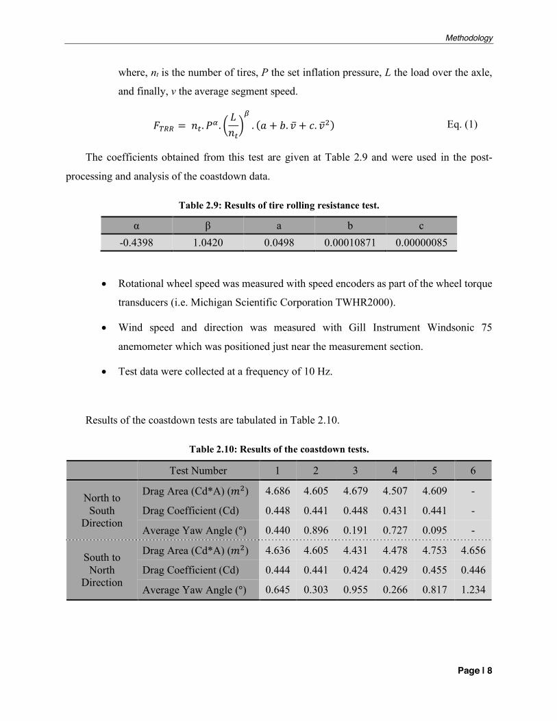
where, nt is the number of tires, P the set inflation pressure, L the load over the axle,

and finally, v the average segment speed.

𝐹011 = 𝑛4. 𝑃7. 8𝐿𝑛4:;

. (𝑎 + 𝑏. �̅� + 𝑐. �̅�)) Eq. (1)

The coefficients obtained from this test are given at Table 2.9 and were used in the post-

processing and analysis of the coastdown data.

Table 2.9: Results of tire rolling resistance test.

α β a b c -0.4398 1.0420 0.0498 0.00010871 0.00000085

• Rotational wheel speed was measured with speed encoders as part of the wheel torque

transducers (i.e. Michigan Scientific Corporation TWHR2000).

• Wind speed and direction was measured with Gill Instrument Windsonic 75

anemometer which was positioned just near the measurement section.

• Test data were collected at a frequency of 10 Hz.

Results of the coastdown tests are tabulated in Table 2.10.

Table 2.10: Results of the coastdown tests.

Test Number 1 2 3 4 5 6

North to South

Direction

Drag Area (Cd*A) (𝑚)) 4.686 4.605 4.679 4.507 4.609 -

Drag Coefficient (Cd) 0.448 0.441 0.448 0.431 0.441 -

Average Yaw Angle (°) 0.440 0.896 0.191 0.727 0.095 -

South to North

Direction

Drag Area (Cd*A) (𝑚)) 4.636 4.605 4.431 4.478 4.753 4.656

Drag Coefficient (Cd) 0.444 0.441 0.424 0.429 0.455 0.446

Average Yaw Angle (°) 0.645 0.303 0.955 0.266 0.817 1.234

Methodology

Page | 9

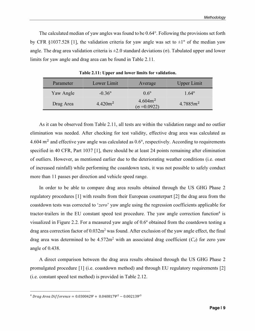
The calculated median of yaw angles was found to be 0.64°. Following the provisions set forth

by CFR §1037.528 [1], the validation criteria for yaw angle was set to ±1° of the median yaw

angle. The drag area validation criteria is ±2.0 standard deviations (σ). Tabulated upper and lower

limits for yaw angle and drag area can be found in Table 2.11.

Table 2.11: Upper and lower limits for validation.

Parameter Lower Limit Average Upper Limit

Yaw Angle -0.36° 0.6° 1.64°

Drag Area 4.420𝑚) 4.604𝑚) (σ =0.0922) 4.7885𝑚)

As it can be observed from Table 2.11, all tests are within the validation range and no outlier

elimination was needed. After checking for test validity, effective drag area was calculated as

4.604 𝑚) and effective yaw angle was calculated as 0.6°, respectively. According to requirements

specified in 40 CFR, Part 1037 [1], there should be at least 24 points remaining after elimination

of outliers. However, as mentioned earlier due to the deteriorating weather conditions (i.e. onset

of increased rainfall) while performing the coastdown tests, it was not possible to safely conduct

more than 11 passes per direction and vehicle speed range.

In order to be able to compare drag area results obtained through the US GHG Phase 2

regulatory procedures [1] with results from their European counterpart [2] the drag area from the

coastdown tests was corrected to ‘zero’ yaw angle using the regression coefficients applicable for

tractor-trailers in the EU constant speed test procedure. The yaw angle correction function4 is

visualized in Figure 2.2. For a measured yaw angle of 0.6º obtained from the coastdown testing a

drag area correction factor of 0.032m2 was found. After exclusion of the yaw angle effect, the final

drag area was determined to be 4.572m2 with an associated drag coefficient (Cd) for zero yaw

angle of 0.438.

A direct comparison between the drag area results obtained through the US GHG Phase 2

promulgated procedure [1] (i.e. coastdown method) and through EU regulatory requirements [2]

(i.e. constant speed test method) is provided in Table 2.12.

4 𝐷𝑟𝑎𝑔𝐴𝑟𝑒𝑎𝐷𝑖𝑓𝑓𝑒𝑟𝑒𝑛𝑐𝑒 = 0.030042𝛹 + 0.040817𝛹) − 0.00213𝛹P

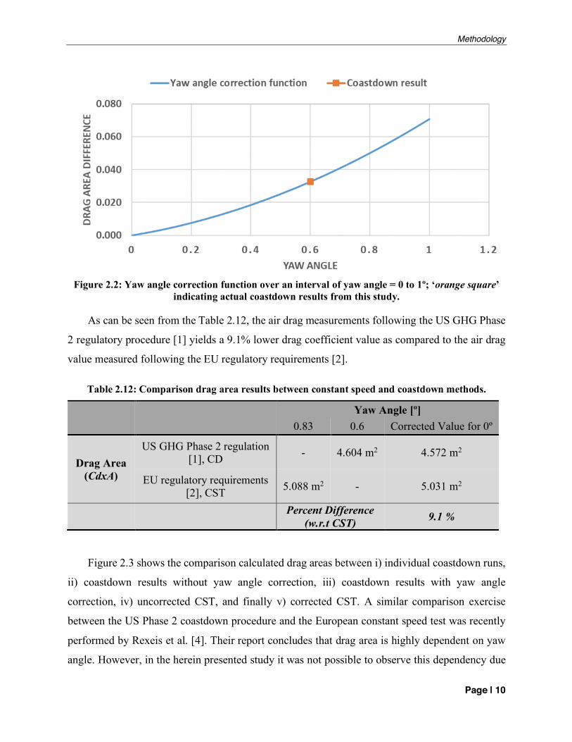
Methodology

Page | 10

Figure 2.2: Yaw angle correction function over an interval of yaw angle = 0 to 1º; ‘orange square’

indicating actual coastdown results from this study.

As can be seen from the Table 2.12, the air drag measurements following the US GHG Phase

2 regulatory procedure [1] yields a 9.1% lower drag coefficient value as compared to the air drag

value measured following the EU regulatory requirements [2].

Table 2.12: Comparison drag area results between constant speed and coastdown methods.

Yaw Angle [º] 0.83 0.6 Corrected Value for 0º

Drag Area (CdxA)

US GHG Phase 2 regulation [1], CD - 4.604 m2 4.572 m2

EU regulatory requirements [2], CST 5.088 m2 - 5.031 m2

Percent Difference (w.r.t CST) 9.1 %

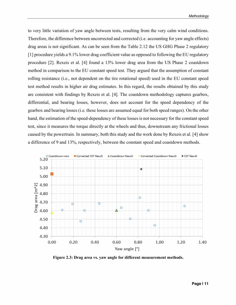
Figure 2.3 shows the comparison calculated drag areas between i) individual coastdown runs,

ii) coastdown results without yaw angle correction, iii) coastdown results with yaw angle

correction, iv) uncorrected CST, and finally v) corrected CST. A similar comparison exercise

between the US Phase 2 coastdown procedure and the European constant speed test was recently

performed by Rexeis et al. [4]. Their report concludes that drag area is highly dependent on yaw

angle. However, in the herein presented study it was not possible to observe this dependency due

Methodology

Page | 11

to very little variation of yaw angle between tests, resulting from the very calm wind conditions.

Therefore, the difference between uncorrected and corrected (i.e. accounting for yaw angle effects)

drag areas is not significant. As can be seen from the Table 2.12 the US GHG Phase 2 regulatory

[1] procedure yields a 9.1% lower drag coefficient value as opposed to following the EU regulatory

procedure [2]. Rexeis et al. [4] found a 13% lower drag area from the US Phase 2 coastdown

method in comparison to the EU constant speed test. They argued that the assumption of constant

rolling resistance (i.e., not dependent on the tire rotational speed) used in the EU constant speed

test method results in higher air drag estimates. In this regard, the results obtained by this study

are consistent with findings by Rexeis et al. [4]. The coastdown methodology captures gearbox,

differential, and bearing losses, however, does not account for the speed dependency of the

gearbox and bearing losses (i.e. these losses are assumed equal for both speed ranges). On the other

hand, the estimation of the speed-dependency of these losses is not necessary for the constant speed

test, since it measures the torque directly at the wheels and thus, downstream any frictional losses

caused by the powertrain. In summary, both this study and the work done by Rexeis et al. [4] show

a difference of 9 and 13%, respectively, between the constant speed and coastdown methods.

Figure 2.3: Drag area vs. yaw angle for different measurement methods.

Methodology

Page | 12

2.3 Chassis dynamometer testing

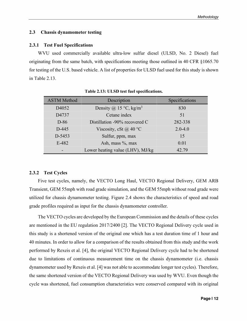
2.3.1 Test Fuel Specifications

WVU used commercially available ultra-low sulfur diesel (ULSD, No. 2 Diesel) fuel

originating from the same batch, with specifications meeting those outlined in 40 CFR §1065.70

for testing of the U.S. based vehicle. A list of properties for ULSD fuel used for this study is shown

in Table 2.13.

Table 2.13: ULSD test fuel specifications.

ASTM Method Description Specifications D4052 Density @ 15 °C, kg/m3 830 D4737 Cetane index 51 D-86 Distillation -90% recovered C 282-338 D-445 Viscosity, cSt @ 40 °C 2.0-4.0

D-5453 Sulfur, ppm, max 15 E-482 Ash, mass %, max 0.01

- Lower heating value (LHV), MJ/kg 42.79

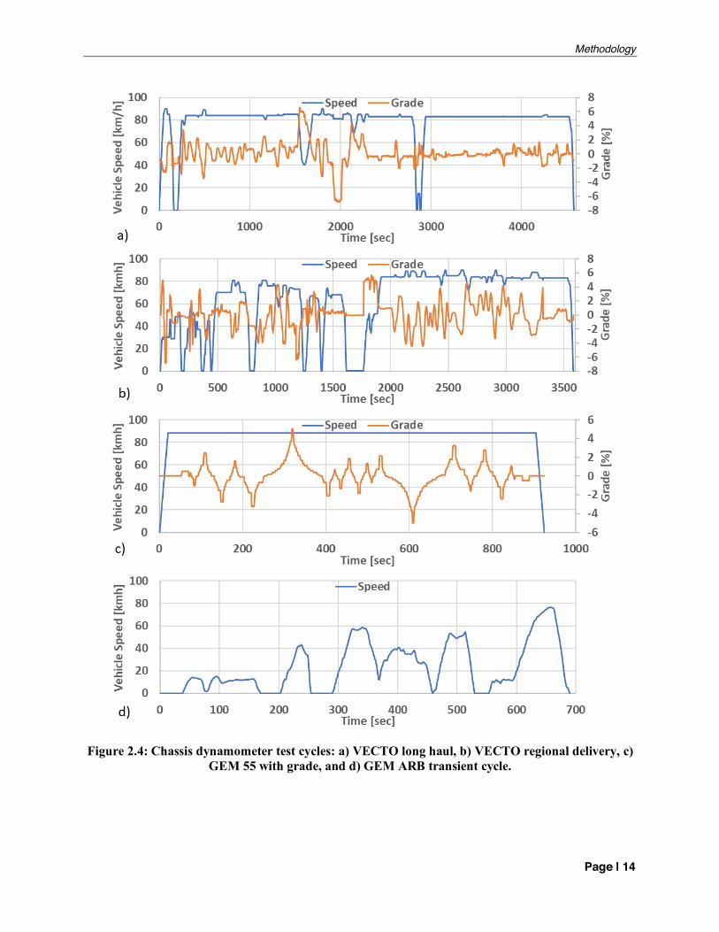
2.3.2 Test Cycles

Five test cycles, namely, the VECTO Long Haul, VECTO Regional Delivery, GEM ARB

Transient, GEM 55mph with road grade simulation, and the GEM 55mph without road grade were

utilized for chassis dynamometer testing. Figure 2.4 shows the characteristics of speed and road

grade profiles required as input for the chassis dynamometer controller.

The VECTO cycles are developed by the European Commission and the details of these cycles

are mentioned in the EU regulation 2017/2400 [2]. The VECTO Regional Delivery cycle used in

this study is a shortened version of the original one which has a test duration time of 1 hour and

40 minutes. In order to allow for a comparison of the results obtained from this study and the work

performed by Rexeis et al. [4], the original VECTO Regional Delivery cycle had to be shortened

due to limitations of continuous measurement time on the chassis dynamometer (i.e. chassis

dynamometer used by Rexeis et al. [4] was not able to accommodate longer test cycles). Therefore,

the same shortened version of the VECTO Regional Delivery was used by WVU. Even though the

cycle was shortened, fuel consumption characteristics were conserved compared with its original

Methodology

Page | 13

cycle. Additional details on the shortening of the VECTO Regional Delivery cycle can be found

in the final project report by Rexeis et al. [4].

The GEM ARB Transient cycle does not include road grade simulation and is used for the

Phase 1 and Phase 2 GHG standards for HDVs in the US. The constant speed cycle, GEM 55mph,

was operated with and without road grade. The GEM 55mph cycle without grade is used in the

Phase 1 certification procedure, whereas the GEM 55mph cycle with grade is used in the

subsequent Phase 2 certification procedure.

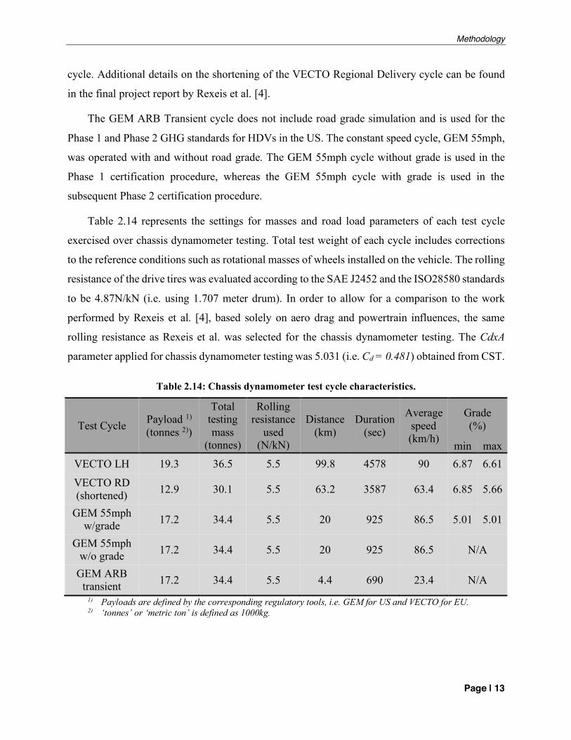
Table 2.14 represents the settings for masses and road load parameters of each test cycle

exercised over chassis dynamometer testing. Total test weight of each cycle includes corrections

to the reference conditions such as rotational masses of wheels installed on the vehicle. The rolling

resistance of the drive tires was evaluated according to the SAE J2452 and the ISO28580 standards

to be 4.87N/kN (i.e. using 1.707 meter drum). In order to allow for a comparison to the work

performed by Rexeis et al. [4], based solely on aero drag and powertrain influences, the same

rolling resistance as Rexeis et al. was selected for the chassis dynamometer testing. The CdxA

parameter applied for chassis dynamometer testing was 5.031 (i.e. Cd = 0.481) obtained from CST.

Table 2.14: Chassis dynamometer test cycle characteristics.

Test Cycle Payload 1) (tonnes 2))

Total testing mass

(tonnes)

Rolling resistance

used (N/kN)

Distance (km)

Duration (sec)

Average speed (km/h)

Grade (%)

min max VECTO LH 19.3 36.5 5.5 99.8 4578 90 6.87 6.61

VECTO RD (shortened) 12.9 30.1 5.5 63.2 3587 63.4 6.85 5.66

GEM 55mph w/grade 17.2 34.4 5.5 20 925 86.5 5.01 5.01

GEM 55mph w/o grade 17.2 34.4 5.5 20 925 86.5 N/A

GEM ARB transient 17.2 34.4 5.5 4.4 690 23.4 N/A

1) Payloads are defined by the corresponding regulatory tools, i.e. GEM for US and VECTO for EU. 2) ‘tonnes’ or ‘metric ton’ is defined as 1000kg.

Methodology

Page | 14

Figure 2.4: Chassis dynamometer test cycles: a) VECTO long haul, b) VECTO regional delivery, c) GEM 55 with grade, and d) GEM ARB transient cycle.

Methodology

Page | 15

2.3.3 Chassis Dynamometer Measurements All chassis dynamometer testing for this study was performed this study using California Air

Resources Board’s (CARB) heavy-duty chassis dynamometer and raw emissions measurement

system stationed at CARB’s Depot Park facility in Sacramento, CA. This section details the chassis

dynamometer and emissions test procedures utilized for the chassis dynamometer testing portion

of this study.

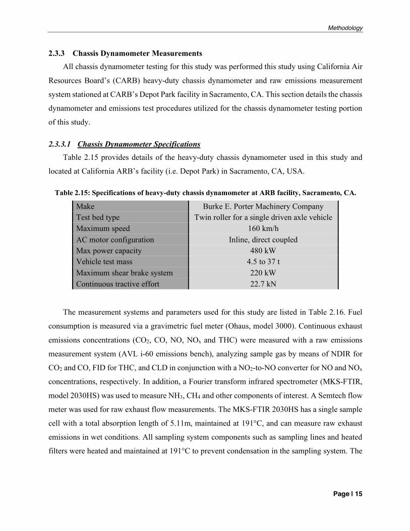
2.3.3.1 Chassis Dynamometer Specifications Table 2.15 provides details of the heavy-duty chassis dynamometer used in this study and

located at California ARB’s facility (i.e. Depot Park) in Sacramento, CA, USA.

Table 2.15: Specifications of heavy-duty chassis dynamometer at ARB facility, Sacramento, CA.

Make Burke E. Porter Machinery Company Test bed type Twin roller for a single driven axle vehicle Maximum speed 160 km/h AC motor configuration Inline, direct coupled Max power capacity 480 kW Vehicle test mass 4.5 to 37 t Maximum shear brake system 220 kW Continuous tractive effort 22.7 kN

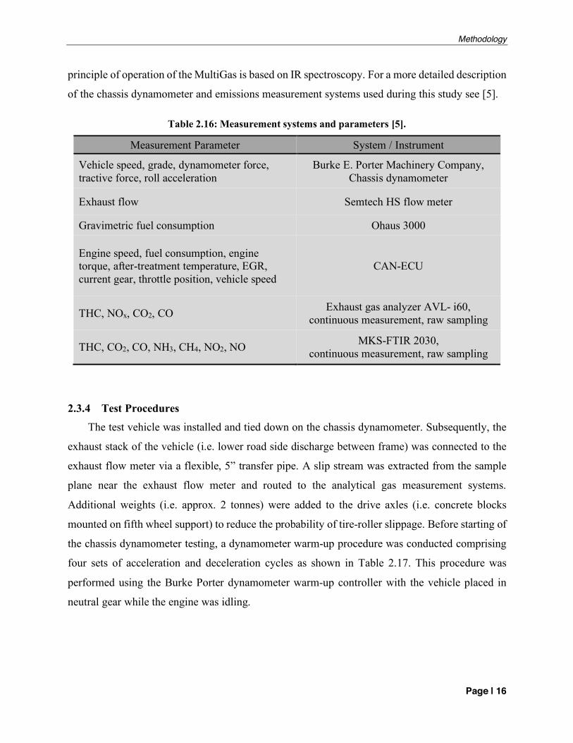
The measurement systems and parameters used for this study are listed in Table 2.16. Fuel

consumption is measured via a gravimetric fuel meter (Ohaus, model 3000). Continuous exhaust

emissions concentrations (CO2, CO, NO, NOx and THC) were measured with a raw emissions

measurement system (AVL i-60 emissions bench), analyzing sample gas by means of NDIR for

CO2 and CO, FID for THC, and CLD in conjunction with a NO2-to-NO converter for NO and NOx

concentrations, respectively. In addition, a Fourier transform infrared spectrometer (MKS-FTIR,

model 2030HS) was used to measure NH3, CH4 and other components of interest. A Semtech flow

meter was used for raw exhaust flow measurements. The MKS-FTIR 2030HS has a single sample

cell with a total absorption length of 5.11m, maintained at 191°C, and can measure raw exhaust

emissions in wet conditions. All sampling system components such as sampling lines and heated

filters were heated and maintained at 191°C to prevent condensation in the sampling system. The

Methodology

Page | 16

principle of operation of the MultiGas is based on IR spectroscopy. For a more detailed description

of the chassis dynamometer and emissions measurement systems used during this study see [5].

Table 2.16: Measurement systems and parameters [5].

Measurement Parameter System / Instrument

Vehicle speed, grade, dynamometer force, tractive force, roll acceleration

Burke E. Porter Machinery Company, Chassis dynamometer

Exhaust flow Semtech HS flow meter

Gravimetric fuel consumption Ohaus 3000

Engine speed, fuel consumption, engine torque, after-treatment temperature, EGR, current gear, throttle position, vehicle speed

CAN-ECU

THC, NOx, CO2, CO Exhaust gas analyzer AVL- i60, continuous measurement, raw sampling

THC, CO2, CO, NH3, CH4, NO2, NO MKS-FTIR 2030, continuous measurement, raw sampling

2.3.4 Test Procedures

The test vehicle was installed and tied down on the chassis dynamometer. Subsequently, the

exhaust stack of the vehicle (i.e. lower road side discharge between frame) was connected to the

exhaust flow meter via a flexible, 5” transfer pipe. A slip stream was extracted from the sample

plane near the exhaust flow meter and routed to the analytical gas measurement systems.

Additional weights (i.e. approx. 2 tonnes) were added to the drive axles (i.e. concrete blocks

mounted on fifth wheel support) to reduce the probability of tire-roller slippage. Before starting of

the chassis dynamometer testing, a dynamometer warm-up procedure was conducted comprising

four sets of acceleration and deceleration cycles as shown in Table 2.17. This procedure was

performed using the Burke Porter dynamometer warm-up controller with the vehicle placed in

neutral gear while the engine was idling.

Methodology

Page | 17

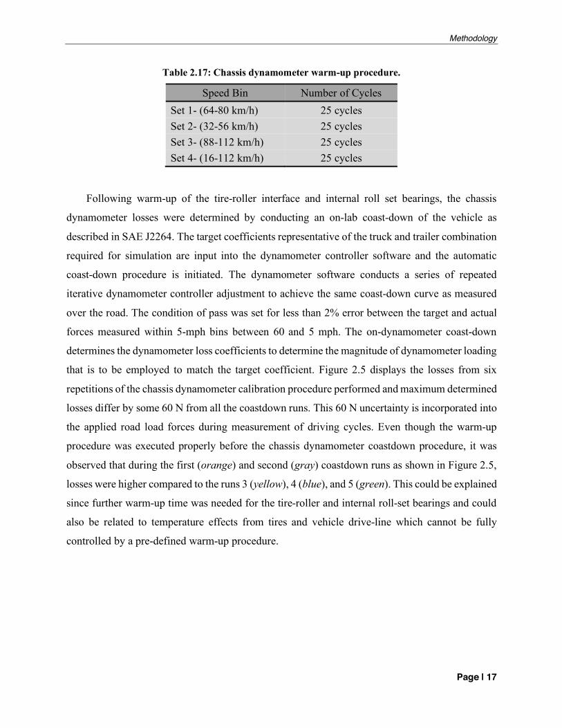
Table 2.17: Chassis dynamometer warm-up procedure.

Speed Bin Number of Cycles Set 1- (64-80 km/h) 25 cycles Set 2- (32-56 km/h) 25 cycles Set 3- (88-112 km/h) 25 cycles Set 4- (16-112 km/h) 25 cycles

Following warm-up of the tire-roller interface and internal roll set bearings, the chassis

dynamometer losses were determined by conducting an on-lab coast-down of the vehicle as

described in SAE J2264. The target coefficients representative of the truck and trailer combination

required for simulation are input into the dynamometer controller software and the automatic

coast-down procedure is initiated. The dynamometer software conducts a series of repeated

iterative dynamometer controller adjustment to achieve the same coast-down curve as measured

over the road. The condition of pass was set for less than 2% error between the target and actual

forces measured within 5-mph bins between 60 and 5 mph. The on-dynamometer coast-down

determines the dynamometer loss coefficients to determine the magnitude of dynamometer loading

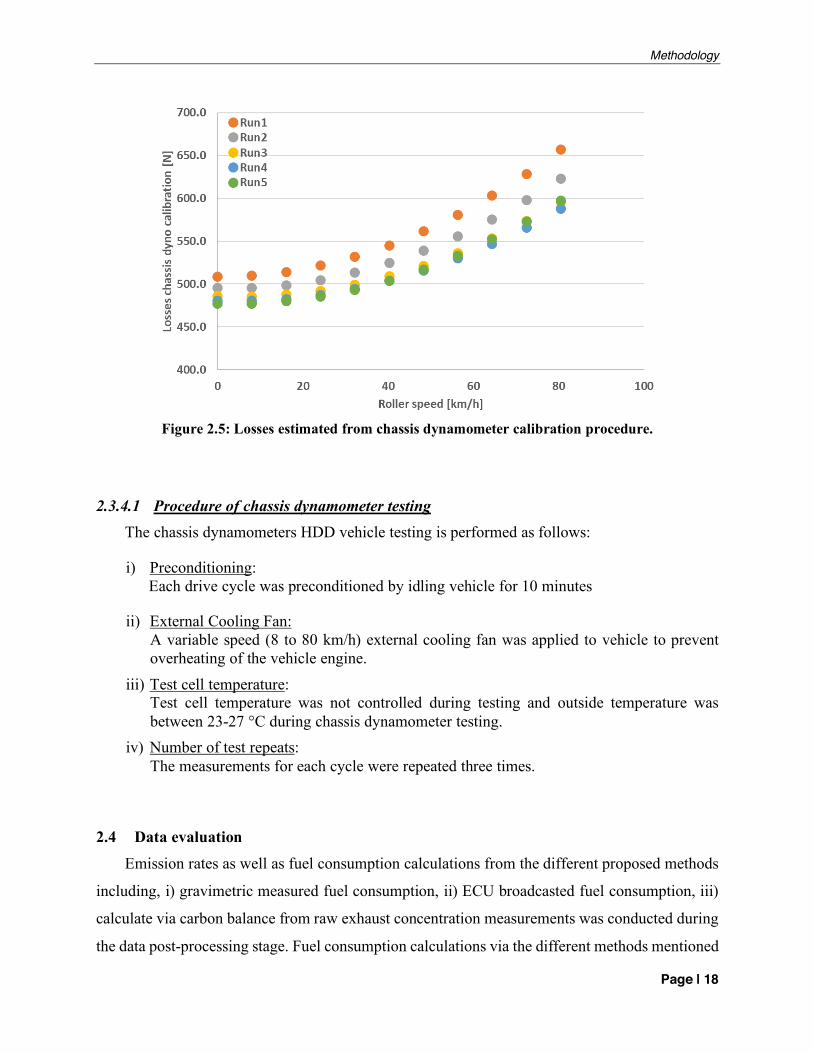
that is to be employed to match the target coefficient. Figure 2.5 displays the losses from six

repetitions of the chassis dynamometer calibration procedure performed and maximum determined

losses differ by some 60 N from all the coastdown runs. This 60 N uncertainty is incorporated into

the applied road load forces during measurement of driving cycles. Even though the warm-up

procedure was executed properly before the chassis dynamometer coastdown procedure, it was

observed that during the first (orange) and second (gray) coastdown runs as shown in Figure 2.5,

losses were higher compared to the runs 3 (yellow), 4 (blue), and 5 (green). This could be explained

since further warm-up time was needed for the tire-roller and internal roll-set bearings and could

also be related to temperature effects from tires and vehicle drive-line which cannot be fully

controlled by a pre-defined warm-up procedure.

Methodology

Page | 18

Figure 2.5: Losses estimated from chassis dynamometer calibration procedure.

2.3.4.1 Procedure of chassis dynamometer testing The chassis dynamometers HDD vehicle testing is performed as follows:

i) Preconditioning: Each drive cycle was preconditioned by idling vehicle for 10 minutes

ii) External Cooling Fan: A variable speed (8 to 80 km/h) external cooling fan was applied to vehicle to prevent overheating of the vehicle engine.

iii) Test cell temperature: Test cell temperature was not controlled during testing and outside temperature was between 23-27 °C during chassis dynamometer testing.

iv) Number of test repeats: The measurements for each cycle were repeated three times.

2.4 Data evaluation

Emission rates as well as fuel consumption calculations from the different proposed methods

including, i) gravimetric measured fuel consumption, ii) ECU broadcasted fuel consumption, iii)

calculate via carbon balance from raw exhaust concentration measurements was conducted during

the data post-processing stage. Fuel consumption calculations via the different methods mentioned

Methodology

Page | 19

was performed for data quality purposes. Calculation of emissions mass rates in [g/s] will follow

recommendations outlined in regulation 40 CFR 1065.650 and include correction for i) transport

delay time in sample lines (i.e. T50 delay time), ii) drift correction for analyzer drift, iii) correction

for removed water content for dry exhaust gas measurements (i.e. NO, NOx, CO2, and CO). Engine

torque and power were calculated based on broadcasted engine control unit (ECU) parameters.

The engine brake torque is not directly broadcasted through ECU and it is determined based

on the parameters broadcasted through the J1939 protocol such as actual engine percent torque

(AEPT), nominal friction torque (NFPT) and engine reference torque. The engine brake torque can

be calculated as shown in Equation 2:

𝑇RSTUV = W(𝐴𝐸𝑃𝑇 − 𝑁𝐹𝑃𝑇) ∗ 𝑇V[\][VSV^VSV[_V4`SabVc/100 Eq. 2

Once the engine brake torque is determined, the engine power and work can be calculated as

shown in Equations 3 and 4, respectively, where Δt is the sampling time in (s), Tbrake, the engine

brake torque (Nm), Pbrake the brake engine power (kW), and Wbrake the engine brake work (kWh).

𝑃RSTUV = 𝑏𝑟𝑎𝑘𝑒4`SabV ∗ 𝑆𝑝𝑒𝑒𝑑 9.5488⁄ Eq. 3

𝑊RSTUV = [𝐸𝑛𝑔𝑖𝑛𝑒k`lVS ∗ ∆𝑡]/3600 Eq. 4

The road-load equation used for the total force applied to the vehicle as shown in Equation 5

where 𝑀4Vq4 is the test mass, a is the acceleration and g is the gravimetric constant. The A term

represents the resistive force that is constant and does not vary with vehicle speed such as tires.

The B term represents the resistive force that varies linearly with vehicle speed such as drivetrain

and differential and the C term represents the resistive force that varies with the square of vehicle

speed such as wind.

𝐹 = [𝐴 + (𝐵 ∗ 𝑉) + (𝐶 ∗ 𝑉))]+ [(1 + 𝑑𝑟𝑖𝑣𝑒𝑎𝑥𝑙𝑒% + 𝑛𝑜𝑛yS]zV𝑎𝑥𝑙𝑒%) ∗ 𝑀4Vq4 ∗ 𝑎]+ [𝑀4Vq4 ∗ 𝑔 ∗ sin(arctan(𝑔𝑟𝑎𝑑𝑒%))]

Eq. 5

Results and Discussion

Page | 1

3 RESULTS AND DISCUSSION 3.1 Average Wheel Work

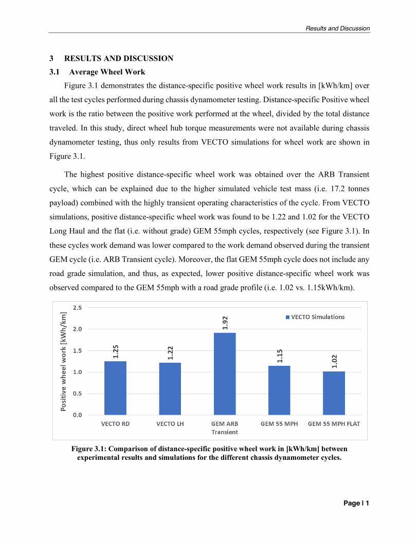
Figure 3.1 demonstrates the distance-specific positive wheel work results in [kWh/km] over

all the test cycles performed during chassis dynamometer testing. Distance-specific Positive wheel

work is the ratio between the positive work performed at the wheel, divided by the total distance

traveled. In this study, direct wheel hub torque measurements were not available during chassis

dynamometer testing, thus only results from VECTO simulations for wheel work are shown in

Figure 3.1.

The highest positive distance-specific wheel work was obtained over the ARB Transient

cycle, which can be explained due to the higher simulated vehicle test mass (i.e. 17.2 tonnes

payload) combined with the highly transient operating characteristics of the cycle. From VECTO

simulations, positive distance-specific wheel work was found to be 1.22 and 1.02 for the VECTO

Long Haul and the flat (i.e. without grade) GEM 55mph cycles, respectively (see Figure 3.1). In

these cycles work demand was lower compared to the work demand observed during the transient

GEM cycle (i.e. ARB Transient cycle). Moreover, the flat GEM 55mph cycle does not include any

road grade simulation, and thus, as expected, lower positive distance-specific wheel work was

observed compared to the GEM 55mph with a road grade profile (i.e. 1.02 vs. 1.15kWh/km).

Figure 3.1: Comparison of distance-specific positive wheel work in [kWh/km] between

experimental results and simulations for the different chassis dynamometer cycles.

Results and Discussion

Page | 2

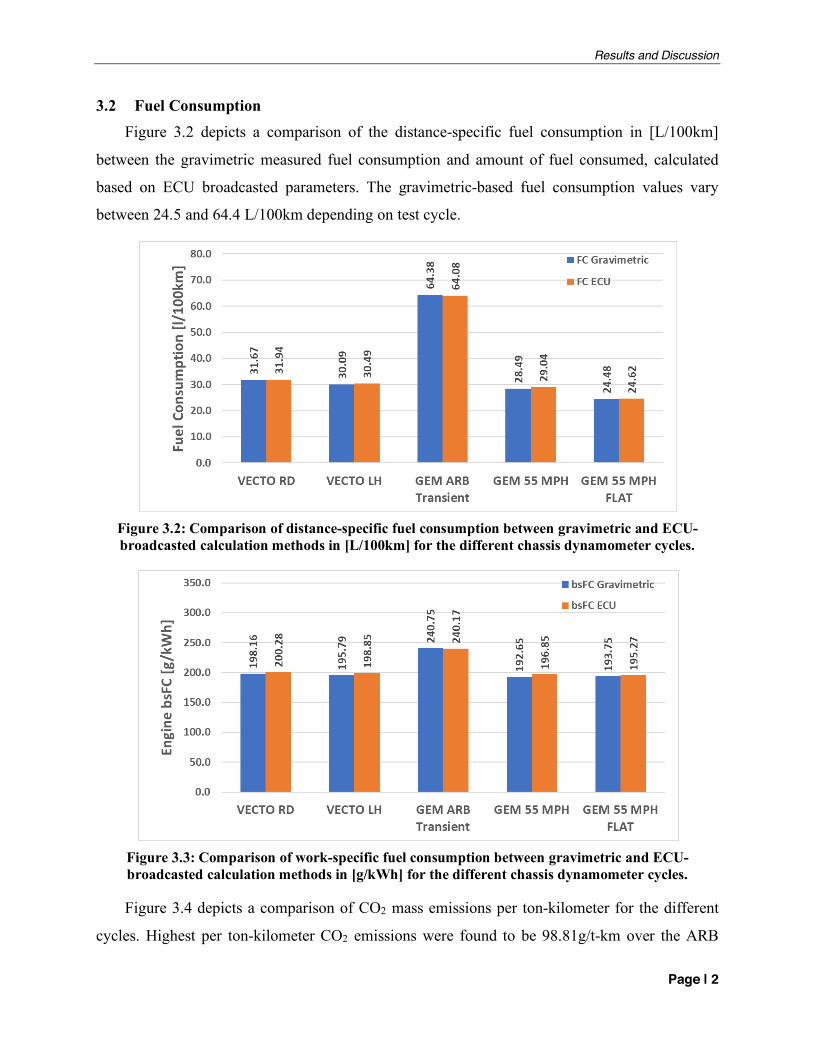
3.2 Fuel Consumption Figure 3.2 depicts a comparison of the distance-specific fuel consumption in [L/100km]

between the gravimetric measured fuel consumption and amount of fuel consumed, calculated

based on ECU broadcasted parameters. The gravimetric-based fuel consumption values vary

between 24.5 and 64.4 L/100km depending on test cycle.

Figure 3.2: Comparison of distance-specific fuel consumption between gravimetric and ECU-broadcasted calculation methods in [L/100km] for the different chassis dynamometer cycles.

Figure 3.3: Comparison of work-specific fuel consumption between gravimetric and ECU-broadcasted calculation methods in [g/kWh] for the different chassis dynamometer cycles.

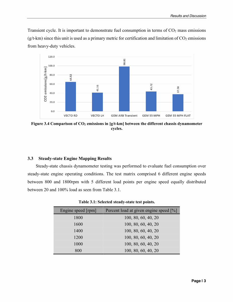
Figure 3.4 depicts a comparison of CO2 mass emissions per ton-kilometer for the different

cycles. Highest per ton-kilometer CO2 emissions were found to be 98.81g/t-km over the ARB

Results and Discussion

Page | 3

Transient cycle. It is important to demonstrate fuel consumption in terms of CO2 mass emissions

(g/t-km) since this unit is used as a primary metric for certification and limitation of CO2 emissions

from heavy-duty vehicles.

Figure 3.4 Comparison of CO2 emissions in [g/t-km] between the different chassis dynamometer

cycles.

3.3 Steady-state Engine Mapping Results Steady-state chassis dynamometer testing was performed to evaluate fuel consumption over

steady-state engine operating conditions. The test matrix comprised 6 different engine speeds

between 800 and 1800rpm with 5 different load points per engine speed equally distributed

between 20 and 100% load as seen from Table 3.1.

Table 3.1: Selected steady-state test points.

Engine speed [rpm] Percent load at given engine speed [%] 1800 100, 80, 60, 40, 20 1600 100, 80, 60, 40, 20 1400 100, 80, 60, 40, 20 1200 100, 80, 60, 40, 20 1000 100, 80, 60, 40, 20 800 100, 80, 60, 40, 20

Results and Discussion

Page | 4

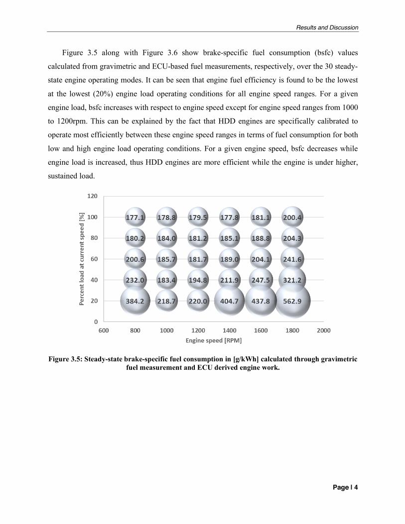
Figure 3.5 along with Figure 3.6 show brake-specific fuel consumption (bsfc) values

calculated from gravimetric and ECU-based fuel measurements, respectively, over the 30 steady-

state engine operating modes. It can be seen that engine fuel efficiency is found to be the lowest

at the lowest (20%) engine load operating conditions for all engine speed ranges. For a given

engine load, bsfc increases with respect to engine speed except for engine speed ranges from 1000

to 1200rpm. This can be explained by the fact that HDD engines are specifically calibrated to

operate most efficiently between these engine speed ranges in terms of fuel consumption for both

low and high engine load operating conditions. For a given engine speed, bsfc decreases while

engine load is increased, thus HDD engines are more efficient while the engine is under higher,

sustained load.

Figure 3.5: Steady-state brake-specific fuel consumption in [g/kWh] calculated through gravimetric

fuel measurement and ECU derived engine work.

Results and Discussion

Page | 5

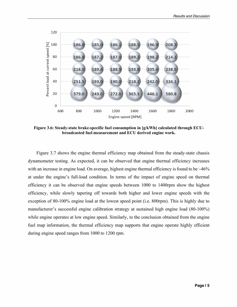
Figure 3.6: Steady-state brake-specific fuel consumption in [g/kWh] calculated through ECU-

broadcasted fuel measurement and ECU derived engine work.

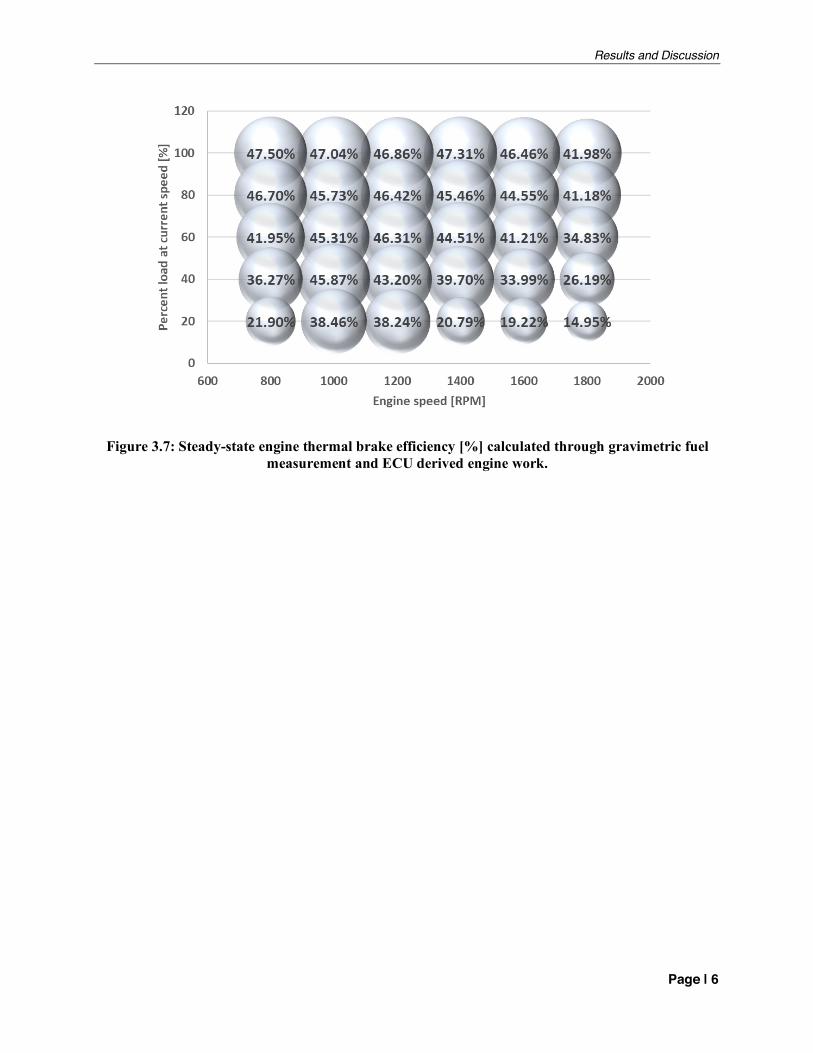
Figure 3.7 shows the engine thermal efficiency map obtained from the steady-state chassis

dynamometer testing. As expected, it can be observed that engine thermal efficiency increases

with an increase in engine load. On average, highest engine thermal efficiency is found to be ~46%

at under the engine’s full-load condition. In terms of the impact of engine speed on thermal

efficiency it can be observed that engine speeds between 1000 to 1400rpm show the highest

efficiency, while slowly tapering off towards both higher and lower engine speeds with the

exception of 80-100% engine load at the lowest speed point (i.e. 800rpm). This is highly due to

manufacturer’s successful engine calibration strategy at sustained high engine load (80-100%)

while engine operates at low engine speed. Similarly, to the conclusion obtained from the engine

fuel map information, the thermal efficiency map supports that engine operate highly efficient

during engine speed ranges from 1000 to 1200 rpm.

Results and Discussion

Page | 6

Figure 3.7: Steady-state engine thermal brake efficiency [%] calculated through gravimetric fuel measurement and ECU derived engine work.

References

Page | 1

4 REFERENCES 1 “Control of Emissions from New Heavy-Duty Motor Vehicles,” US Environmental Protection

Agency, Federal Register, Title 40, Vol. 1037, Subpart F, §1037.528, accessed: April, 2018. 2 European Commission. (2017). REGULATION (EU) 2017/2400 of 12 December 2017

implementing Regulation (EC) No 595/2009 of the European Parliament and of the Council as regards the determination of the CO2 emissions and fuel consumption of heavy-duty vehicles and amending Directive 2007/46/EC of the European Parliament and of the Council and Commission Regulation (EU) No 582/2011. Official Journal of the European Union, L 349. Retrieved from http://eur-lex.europa.eu/legal-content/EN/TXT/?uri=OJ:L:2017:349:TOC.

3 “Control of Emissions from New Heavy-Duty Motor Vehicles,” US Environmental Protection Agency, Federal Register, Title 40, Vol. 1037, Subpart F, §1037.501, accessed: April, 2018.

4 Rexeis, M., Röck, M., and Hausberger, S. (2018). Comparison of fuel consumption and emissions for representative heavy-duty vehicles in Europe (No. FVT-099/17/Rex EM 16/18-6790). Technische Universität Graz. Retrieved from https://www.theicct.org/publications/HDV-EU-fuel-consumption-and-emissions-comparison.

5 Arvind Thiruvengadam et al., “Cross Correlation of ARB Heavy-Duty Chassis Dynamometer Emissions Laboratory with WVU Transportable Emissions Measurement System (TEMS),” Final Project Report, Contract Number 12-536, August, 19th, (2016).