What is the Probability of a Recession in the United States?

Department of Economics Lund University, Sweden M.Sc. Thesis 2006 September Author: Daniel Ekeblom Instructor: Kristian Jönsson

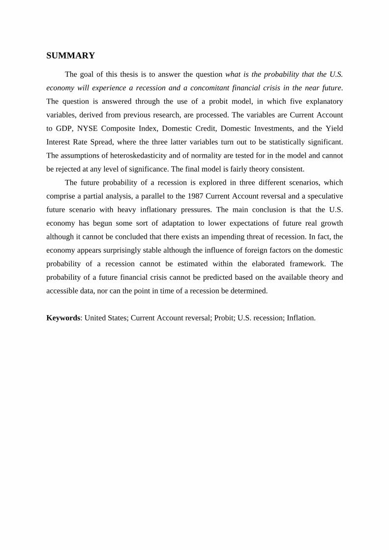
SUMMARY

The goal of this thesis is to answer the question what is the probability that the U.S.

economy will experience a recession and a concomitant financial crisis in the near future.

The question is answered through the use of a probit model, in which five explanatory

variables, derived from previous research, are processed. The variables are Current Account

to GDP, NYSE Composite Index, Domestic Credit, Domestic Investments, and the Yield

Interest Rate Spread, where the three latter variables turn out to be statistically significant.

The assumptions of heteroskedasticity and of normality are tested for in the model and cannot

be rejected at any level of significance. The final model is fairly theory consistent.

The future probability of a recession is explored in three different scenarios, which

comprise a partial analysis, a parallel to the 1987 Current Account reversal and a speculative

future scenario with heavy inflationary pressures. The main conclusion is that the U.S.

economy has begun some sort of adaptation to lower expectations of future real growth

although it cannot be concluded that there exists an impending threat of recession. In fact, the

economy appears surprisingly stable although the influence of foreign factors on the domestic

probability of a recession cannot be estimated within the elaborated framework. The

probability of a future financial crisis cannot be predicted based on the available theory and

accessible data, nor can the point in time of a recession be determined.

Keywords: United States; Current Account reversal; Probit; U.S. recession; Inflation.

TABLE OF CONTENTS

1 INTRODUCTION .......................................................................................................... 2

2 PREVIOUS RESEARCH............................................................................................ 4

2.1 THE U.S. CURRENT ACCOUNT AND THE U.S. NIIP ............................................................................ 4 2.2 FINANCIAL CRISES ............................................................................................................................. 8

3 EMPIRICAL METHODOLOGY............................................................................ 14

3.1 THE PROBIT MODEL......................................................................................................................... 14 3.1.1 Specification Issues ................................................................................................................. 16 3.1.2 Out-of-sample Prediction ........................................................................................................ 18 3.1.3 Testing Strategy....................................................................................................................... 19

3.2 DATA ............................................................................................................................................... 20 3.2.1 Dependent Variables ............................................................................................................... 21 3.2.2 Explanatory Variables............................................................................................................. 22 3.2.3 Excluded Variables ................................................................................................................. 25

4 RESULT ..................................................................................................................... 30

4.1 THE FINAL MODEL........................................................................................................................... 34 4.1.1 Marginal Effects ...................................................................................................................... 35

5 ANALYSIS ................................................................................................................. 39

5.1 PARTIAL ANALYSIS.......................................................................................................................... 40 5.2 PARALLEL TO THE CURRENT ACCOUNT REVERSAL IN 1987............................................................. 42 5.3 INFLATIONARY PRESSURES .............................................................................................................. 44

6 CONCLUSION .......................................................................................................... 49

7 FURTHER RESEARCH........................................................................................... 51

REFERENCES.............................................................................................................. 54

INTERNET REFERENCES........................................................................................ 59

APPENDIX A................................................................................................................ 60

TABLES AND FIGURES

TABLE 3.1: CROSS-TABULATION TABLE OF ACTUAL AND PREDICTED OUTCOMES..................... 19

FIGURE 3.1: CORRELATION OF THE 3 MONTH U.S. TREASURY SECURITY AND THE DISCOUNT

WINDOW PRIMARY CREDIT RATE ........................................................................ 29

TABLE 4.1: DENOTATIONS OF EXPLANATORY VARIABLES ......................................................... 30

TABLE 4.2: FIRST SEQUENCE OF COMPUTATIONS....................................................................... 30

TABLE 4.3: SECOND SEQUENCE OF COMPUTATIONS................................................................... 31

TABLE 4.4: THIRD SEQUENCE OF COMPUTATIONS...................................................................... 32

TABLE 4.5: FOURTH SEQUENCE OF COMPUTATIONS................................................................... 33

TABLE 4.6: FIFTH SEQUENCE OF COMPUTATIONS ...................................................................... 33

TABLE 4.7: THE FINAL MODEL................................................................................................... 34

TABLE 4.8: MARGINAL EFFECTS OF THE VARIABLES OF THE FINAL MODEL ............................... 36

FIGURE 4.1: IN-SAMPLE PREDICTION BY FINAL MODEL. ACTUAL SERIES OF DEPENDENT

VARIABLE Y4 (Y), AND FITTED PROBABILITIES (Ŷ). ................................................ 38

FIGURE 5.2.1: CURRENT ACCOUNT TO GDP – 1987 CURRENT ACCOUNT REVERSAL................ 42

FIGURE 5.2.2: INTEREST RATE SPREAD – 1987 CURRENT ACCOUNT REVERSAL ....................... 42

FIGURE 5.2.3: NYSE – 1987 CURRENT ACCOUNT REVERSAL ................................................... 43

FIGURE 5.2.4: DOMESTIC CREDIT – 1987 CURRENT ACCOUNT REVERSAL ................................ 43

FIGURE 5.2.5: DOMESTIC INVESTMENTS – 1987 CURRENT ACCOUNT REVERSAL...................... 43

FIGURE 5.2.6: FITTED PROBABILITIES – 1987 CURRENT ACCOUNT REVERSAL.......................... 43

FIGURE 5.3.1: CURRENT ACCOUNT TO GDP – INFLATIONARY PRESSURES................................ 47

FIGURE 5.3.2: INTEREST RATE SPREAD – INFLATIONARY PRESSURES ....................................... 47

FIGURE 5.3.3: NYSE – INFLATIONARY PRESSURES ................................................................... 47

FIGURE 5.3.4: DOMESTIC CREDIT – INFLATIONARY PRESSURES ................................................ 47

FIGURE 5.3.5: DOMESTIC INVESTMENTS – INFLATIONARY PRESSURES...................................... 47

FIGURE 5.3.6: FORECASTED PROBABILITIES – INFLATIONARY PRESSURES ................................ 47

FIGURE 5.3.7: COMPARISON OF FORECASTED PROBABILITIES (MODEL 5.3) AND COMPUTED

PROBABILITIES (MODEL 5.2) ON THE 1987 CURRENT ACCOUNT REVERSAL. ...... 48

1

1 Introduction

A concern for the state of the U.S. economy and implicitly the world economy has

steadily been growing for some time. This concern originates from the financial predicament

of the U.S. economy, i.e. the U.S. dependence on foreign capital to notably fuel domestic

consumption. Opinions have been raised that the U.S. investment relationship with the rest of

the world is likely to be untenable (IMF 2002; Mann 2002). The Current Account deficit

amounts to approximately 6% of GDP on an annual basis and the net international investment

position deficit is equivalent to approximately a quarter of the U.S. GDP (Bureau of

Economic Analysis, 2006). In addition to this perceived predicament the U.S. experience low

private savings rates and a budget deficit that probably will exceed at least 10% of GDP over

the future 50 years (Congressional Budget Office, 2003). The situation is alleged to be – or

soon to be – dire, based on various degrees of indications for the U.S. whose domestic

consumption far outweighs domestic production.

The opinions mirroring a general outlook for the U.S. economy, and causing the debate,

can be summarized by Levey and Brown (2005). The accumulation of foreign debt is

unsustainable in the long term. At a certain point, i.e. when total net foreign liabilities have

reached such a level that foreign investors are reluctant to invest further in the U.S. economy

due to altered expectations on future earnings, the process of accumulating debt has to

reverse. The reversal of the U.S. debt accumulation and consequently the Current Account

deficit would, in an implausible scenario according to Levey and Brown (2005, p. 2), “set off

a panic, causing the dollar to tank, interest rates to skyrocket, and the U.S. economy to

descend into crisis, dragging the rest of the world down with it”. The purpose of the debate

can be said to clarify whether such a scenario is probable and if so, to pinpoint the date when

these events will occur. In the light of recent discussion, I pose the question what is the

probability that the U.S. economy will experience a recession and a concomitant financial

crisis in the near future?

In the second chapter I will account for previous research and the nature of the matter.

The following subjects will be treated in two subchapters: the sustainability of the Current

Account deficit and the closely related importance of the net international investment

position; the nature of and the occurrence of financial crises and likely causes. The third

chapter contains a presentation of the theory and the probit model elaborated in order to assist

in answering the question. An account of the data motivated by previous research and a

testing strategy of the model is also presented in the chapter. The fourth chapter accounts for

2

the results of the computation of the final model. Coefficients, significances, and marginal

effects of the explanatory variables will be presented along with the measure-of-fit. In the

fifth chapter the model is applied to various scenarios in order to explore the probability of

recession for the U.S. economy. A conclusion will follow in the sixth chapter where I

basically state that the probability for a U.S. recession is rather low under accompanying

assumptions. A subchapter suggests interesting aspects which may make up future research.

3

2 Previous Research

The problem as formulated by Levey and Brown (2005) consists of two parts. First of

all, the main sources of concern for the state of the U.S. economy would be the negative Net

International Investment Position (from now on referred to as the NIIP) and the Current

Account deficit, which are intimately interdependent1. Secondly, a chain of events that would

supposedly lead to a situation where the “Sudden unwillingness by investors abroad to

continue adding to their already large dollar assets, in this scenario, would set off a

panic,…” (Levey, Brown, 2005 p. 2).

The concerns that a possibility for domestic imbalances exist in U.S. fundamentals are

not new and previous research has dealt with these issues in numerous ways. In order to

establish previous findings, conventional accords and disputes, I will account for the various

positions on the U.S. Current Account deficit and the U.S. NIIP in subchapter 2.1. The

recapitulation is supposed to shed light on the premier part of the issue with respect to the

probability of a future recession. Secondly, I will make an account of previous research on

financial crises in subchapter 2.2 in order to hopefully complete the composition of the entire

issue. The chapter on Previous Research is deliberately concise because it spans a very large

subject. It is purely intended to supply the reader of an orientation from which further

inquiries may be maid.

2.1 The U.S. Current Account and the U.S. NIIP

The issue of a sustainable Current Account deficit thus includes the aspect of a

manageable NIIP2. The definition of sustainable Current Account deficit is well characterized

by Mann (2002, p. 143): “…the external imbalance generates no economic forces that change

its trajectory”. When the Current Account deficit is large it indicates a growing negative

NIIP. If the financial costs – interest and dividends – sustaining the negative NIIP become

1 A negative NIIP implies that the U.S. is left with net foreign liabilities when U.S. assets possessed by

foreigners (external liabilities) have been deducted from foreign assets owned by U.S. residents (external assets).

The Current Account is correlated to the NIIP in the sense that a Current Account deficit implies a capital

account surplus by definition, which in turn signifies that U.S. residents are either selling of U.S. assets to

foreigners – implicitly reducing external assets - or borrowing foreign capital i.e. accumulating external

liabilities. 2 For a more elaborate description of different perspectives on the US Current Account deficit, see Mann (2002).

4

sufficiently large they will eventually cut into current consumption and investments,

consequently reducing growth and making the present level unsustainable (Mann, 2002).

However, a large negative NIIP does not have to be an ominous signal. The accumulation of

foreign liabilities would not be possible if it were not for other countries’ confidence in the

U.S. economy (Cooper, 2001).

A large Current Account deficit does not necessarily result in a deteriorating NIIP over

time. If the inflow of foreign capital generates productivity growth it will also increase the

long term GDP growth. It is possible that a higher growth of real GDP facilitates the

upholding of a negative NIIP without considerably affecting current consumption and

investments (Miles-Ferreti, Razin, 1996). To establish a feasible level of foreign investments

in the U.S. economy that global investors are ready to support is nonetheless hard based on

the share of U.S. assets in the global investor’s portfolio (Meade, Thomas, 1993; Ventura,

2001), and perhaps even inadequate as a measure of sustainability for that matter.

Some voices have suggested that the Current Account is misleading as a measure of the

evolution of the NIIP. Obstfeld (2004, p. 564) claims that “National portfolios are

increasingly leveraged through the trade of claims on the home country for claims on

foreigners, trades that need not entail any change in national wealth at the point securities

change hands”. The real exchange of wealth could occur at some point later in time, after the

switch of financial assets has taken place. The exchange of securities remains a formal

accounting procedure, not necessarily analogous to an exchange of real values. Further,

Obstfeld (2004) argues that attempts to exploit the Current Account-to-NIIP nexus by running

increasingly larger deficits in order to instigate a Current Account reversal might result in a

collapse of whatever statistical regularity that has existed in the past. It is basically the Lucas-

critique3 applied to another context.

The U.S. NIIP may fluctuate with changes in the value of the present external assets and

liabilities due to volatility in asset prices or exchange rates, which may cause an exaggerated

concern for the state of the U.S. economy (Tille, 2003). In 2001, the U.S. net international

debt leaped to approximately $2.3 trillion, from half the level recorded in 1999. The increase

reflected the additional borrowing undertaken by the U.S. to finance the rising Current

Account deficit. Nevertheless, a third of the change was traced to the effect of a rising dollar

on the value of U.S. external assets. Although being purely nominal adjustments in the U.S.

NIIP, they do not prevent the occurrence of real effects on economic activity if unknown to

3 See Lucas (1976) for an exposition.

5

the public (Barro, 1976). In the case where the market does not have complete information on

the matter, future expectations will be conceived on false grounds and the purely nominal

adjustments will result in real effects.

Furthermore, the Euro was introduced in 1999 and this event altered the financial

conditions for the U.S. economy. The lack of integration of the European financial markets

made it more costly for international investors to obtain European exposure in the matter of

risk management. The slower growth in the euro area most certainly added to the

unwillingness of investors to hold the euro. Consequently, capital inflows to Europe were

lower than they otherwise might be, and these events prevented the euro from appreciating

even further via-a-vis the dollar (BIS, 2002; IMF 2001).

Empirical findings strongly suggest that the U.S. income elasticity for imports of goods

and services is significantly greater than the foreign income elasticity for U.S. exports of

goods and services. These findings are consistent over different periods, data, and

econometric techniques (Houthakker, Magee, 1969; Cline, 1989; Hooper, Johnson, Marquez,

1998; Wren-Lewis, Driver, 1998). They also entail a continuously expanding Current

Account deficit if the U.S. economy and the rest of the world grow at an equivalent pace,

unless the dollar persistently depreciates (Krugman, 1985; Krugman, Baldwin, 1987;

Obstfeld, Rogoff, 2000). A study by the IMF (2004) finds nearly identical output growth rates

for the U.S. and its export-weighted partners from the 1990s and forth. The dollar has not

depreciated as the present state of the Current Account would suggest and the historical trend

appreciation most likely mirrors the unrivalled U.S. productivity growth in reference to other

major industrialized economies (Marston, 1987; Tille et al, 2001; Alquist, Chinn, 2002).

The ‘true’ value of the dollar is subject to much controversy. Some proponents claim

that a rather abrupt depreciation of the dollar which in turn facilitates the diminution of the

Current Account deficit is a likely scenario in the near future. According to Blanchard et al

(2005) the dollar is bound to depreciate, but the pace of the depreciation is conditional on the

degree of substitutability between U.S. assets and foreign assets. The current slow rate of

depreciation thus suggests that assets lack substitutability. Poor development of financial

markets in Asia and the need to accumulate international collateral implies an increasing

relative demand for U.S. assets. Chinese investors, currently limited by capital controls,

constitute a latent demand for U.S. assets, which may further alter the conditions for currency

equilibrium when unleashed (Dooley et al, 2004; Caballero et al, 2005).

A seminal analogy to the Bretton Woods system was introduced by Dooley, Folkerts-

Landau and Garber in 2003 (Dooley et al, 2003). The appearance of a fixed exchange rate

6

periphery in Asia (China, Taiwan, HK, Singapore, Japan, Korea, and Malaysia) has once

again established the U.S. as the centre in a Bretton-Woods similar international monetary

system. The strategy of the Asian countries is to stimulate growth through the exports

supported by an undervalued fixed exchange rate and capital controls. The accumulation of

reserve assets serve as an increasing financial claim on the centre country, implicitly

strengthening the dollar. The economic growth thus allows the periphery to graduate to the

centre for an extensive period of time, as the countries of Europe once did under the original

Bretton-Woods system.

Albeit relevant for the elucidation of the dollars strength and the U.S. Current Account

deficit, the Bretton-Woods analogy constitutes yet another disputed explanation to the

emergence of the U.S. Current Account deficit. Even the original Bretton-Woods system was

controversial and much criticized. Once again actualized, Triffin’s Dilemma stated that if the

U.S. seized to run a balance of payments deficit, the international community would lose its

largest source of additions to reserves (Triffin, 1960). The ensuing shortage of liquidity could

cause instability in the world economy through its contractionary effect. But if the U.S. would

continue to fuel world economic growth through its balance of payments deficit, the excessive

U.S. deficits would reduce confidence in the value of the dollar, and it would risk being

refused as the global reserve currency. Bretton-Woods could break down, leading to

instability on a global scale.

Eichengreen (2004) and Roubini and Setser (2005) argue that current state of affairs is

not sustainable. There are several reasons for such unravelling of events, but the mutual

critique lies in structural differences: the world has changed a great deal the last thirty years

and it is simply not possible to talk of a revived Bretton-Woods. Roubini and Setser (2005)

also stresses that the sheer size of the U.S. Current Account deficit is intractable. The side

effects – such as unsuccessful sterilization operations and a possible loss on investments – of

Asian central banks’ attempts to fund it will bring about an end of the revived Bretton-Woods.

Obstfeld and Rogoff (2004) argue that the current conjuncture of the U.S. economy resembles

the early 1970s, when the Bretton Woods system collapsed.

Empirical evidence suggests that the long term Current Account/GDP ratio is

statistically stationary (Taylor, 2002). A large Current Account deficit may be expected to

decline in comparison to its long term mean, whereas a small Current Account deficit is a

candidate for possible growth. Freund (2000) identifies a 5% Current Account/GDP threshold

beyond which Current Account reversals typically occur. Main characteristics of a reversal

are a significant slowdown in output growth, a 10–20% real depreciation of the domestic

7

currency, a subsequent increase in real export growth, a decline in Domestic Investments, a

small reduction of the budget deficit and some levelling off in the NIIP.

Debelle and Galati (2005) have completed a study of Current Account adjustments in

industrialized countries and their findings are in line with previous research. Current Account

reversals were typically associated with a sizeable slowdown in domestic growth,

investments, and large exchange rate depreciation. These findings are also corroborated by

Edwards (2004). Credit growth had a propensity to increase before and to peak one year after

the Current Account adjustment. The inflation profile – inflation typically declined by several

percentage points – presumably signalled the presence and a following resolution of

macroeconomic imbalances. Debelle and Galati (2005) argue that causality is not explained

by these types of econometric studies and that the question whether Current Account

adjustments are exogenous or endogenous to these development remains unanswered. A

plausible explanation of their own is that Current Account reversals in such episodes reveal

the expansion and resolution of national economic imbalances.

The multiple perspectives on the Current Account deficit as such reflect the complexity

of the matter, and that few conventional positions remain. There is some accord on the size of

the U.S. Current Account deficit and the U.S. NIIP: they are unusually large and a probability

exists – yet undefined – that they will regress. However, the pace of the reversal is subject to

debate. A number of indicators, such as the Current Account to GDP ratio, output growth,

exports, domestic investments, and the value of the dollar possibly presage Current Account

reversals. But even a relatively large Current Account deficit provides no definite indication

of the probability of a reversal, nor of the stability of the domestic economy.

2.2 Financial Crises

Financial crises occur regularly and cyclically (Kindleberger, 1996), and they seldom

occur in combination with healthy economic fundamentals (Kaminsky, Reinhart, 1999; Borio,

Lowe, 2002). There have been made several definitions of a financial crisis throughout the

history of financial research and several key components have been identified, but I favour the

somewhat simplistic definition by Bordo et al (2001, p. 55): “…episodes of financial-market

volatility marked by significant problems of illiquidity and insolvency of financial-market

participants and/or by official intervention to contain such consequences”. Bordo et al (2001,

p. 55) further divide financial crises into banking crisis – “…financial distress resulting in the

erosion of most or all of aggregate banking system capital” - and currency crisis – “…a

8

forced change in parity, abandonment of a pegged exchange rate, or an international

rescue”.

The explanation that financial globalization is a leading cause for the occurrence of

currency crises lacks support (Bordo et al, 2001). A lesser frequency of currency crises in the

pre-1913 and post-1972 periods, when capital controls were absent and capital mobility

prevalent, disputes the view that financial globalization has created instability in foreign

exchange markets. Tight regulations of domestic and international capital markets suppressed

banking crises almost completely in the 1950s and 1960s, whereas capital controls were

deficient in suppressing currency crises. Furthermore, data indicates that currency crises tend

to be an emerging-market problem in particular.

Attempts have been made to quantify the loss of a financial crisis. The output loss,

calculated as the sum of the differences from the commencement of the crisis to the recovery

between pre-crisis trend growth and actual growth, is roughly ten percentage points larger in

recessions with crises than in recessions without them both since 1973 and before 1913

(Bordo et al, 2001). The cost of currency crises does not appear to be determined by the

domestic budget balance, financial system, or exchange rate regime, but the Current Account

deficit does seem to matter. The cost is greater when the Current Account deficit deepens

significantly in the preceding period for post-1972 period. Currency crises also become more

costly in conjunction with banking-sector problems (Kaminsky, Reinhart, 1999). These

calculations might overstate the loss because pre-crisis growth tends to be unsustainably high,

making it less appropriate for comparison (Mulder, Rocha, 2000). Furthermore, not all crises

identified by Bordo et al (2001) are correlated with loss of output. Since crises often occur in

recessions, it could be that computed output losses are merely normal contractionary effects.

According to Boyd et al (2005) there is a non negligent possibility that banking crises

engender no loss of economic output in highly developed economies. This particular finding

renders it supposedly even more difficult to econometrically relate loss of output during

financial crises to explanatory variables.

Banking crises tend to correlate with liquidity support for insolvent banks and the nature

of the exchange rate regime. The reason for open-ended liquidity support to increase the cost

of crises is evident. Public liquidity support to banks that is not conditional on restructuring

and recapitalization permit insolvent institutions to opt for gratuitous resurrection. They

9

facilitate the continued flow of capital to loss-making borrowers and allow owners and

managers to engage in stealing company property4 (Akerlof, Romer, 1993).

Banking crises tend to build up over time and to be the result of deteriorating economic

fundamentals (Borio, Lowe, 2002). Banking crises associated with significant loss of output

often occur in conjunction with the exposure of several institutions to a number of risk

factors. A common scenario in which banking crises occur is an expanding economy with

increasing prices on assets such as real estate and equity, where risk is perceived to decline

and external financing becomes cheaper. Therefore, the build-up of financial imbalances

should be possible to discern in the appreciation of the real exchange rate, capital inflows, and

the potential build-up of concomitant foreign exchange mismatches. An important note is that

banking crises normally propagates through deteriorating asset quality5. Borio and Lowe

(2002) identify three core variables which are perceived to indicate the presence of such

imbalances: the ratio of private sector credit to GDP, equity prices deflated by the price level,

and the real effective exchange rate. To capture the cumulative processes indicating the level

of financial distress, they compute the deviations of core variables from a Hodrick-Prescott

trend. If the indicators exceed some critical threshold, then financial imbalances are assumed

to be emerging and signalling the risk of ensuing financial distress. The variables, i.e. the

cumulative deviations from the trend, allow for variable forecasting horizons. A good

indicator would consequentially have a low noise-to signal ratio, predicting a high fraction of

the crises that occur but not turn on too often implicitly signalling crises that do not

materialise. The exchange rate indicator might be more valid in emerging market economies.

These tend to rely more on external finance and they often have fixed exchange rate regimes.

Borio and Lowe (2002) find that the credit level and asset price combination is a superior

indicator to the credit level and exchange rate alternative, and if the equity price gap is

included then the exchange rate does not apparently add useful information. Studies on rapid

credit growth suggest the higher the growth rate is in a business cycle upswing the more

decisive is the contraction in the downswing (Gavin, Hausmann, 1996). Credit escalation is

also a reliable indicator of subsequent banking crises (Caprio et al, 1994).

4 The behaviour is also a symptom of the Soft Budget Constraint syndrome (Kornai et al, 2003)

5 This is a partial symptom of a credit crunch where too small a share of equities to detain the consequence of

bankruptcy instigates the propagation process. For a further exposition on credit crunches, see (Bernanke, Lowe,

1991; Yuan, Zimmerman, 1999).

10

Due to the heterogeneous nature of crises it is unlikely that attempts to statistically

relate them to fundamentals will have high explanatory power (Eichengreen et al, 1995). This

view could be interpreted as if there is a psychological or an unquantifiable component to a

crisis. The idea that international capital markets are a source of market discipline is flawed

their arbitrary and erratic history (Eichengreen, 2000). A herding behaviour amongst

international investors can be rational when information is scarce. Agents then infer

information from the actions of other agents and therefore behave similarly (Calvo, Mendoza,

1997). Incomplete, or asymmetric, information is a prerequisite for such a scenario where ill-

informed investors infer that a security is of a different quality than previously assumed from

the decisions of other investors. They act collectively – by buying or selling -amplifying price

movements and precipitating crises. Financial globalization is contributing to herding and

thereby financial volatility as the increase in the menu of available assets floods international

investors with investment alternatives without necessary complementary information. The

result is an increase in tendency for incomplete-information problems. Whether these

problems are causal or symptomatic of investors’ behaviours is hard to identify. There are

examples when international investors who willingly overlook weaknesses in domestic policy

environments until they are abruptly revealed cause overreaction and panic amongst creditors,

which may result in a disproportionately severe financial crisis for the country (Calvo,

Mendoza, 1996).

According to Mishkin (1996b, p. 10) asymmetric information theory define a financial

crisis as: “…a nonlinear disruption to financial markets in which adverse selection and moral

hazard problems become much worse, so that financial markets are unable to channel funds

efficiently to those who have the most productive investment opportunities”. In the case of

imperfect knowledge of borrower quality, the problem of adverse selection can occur.

Incomplete information prevents lenders from evaluating credit quality. As a result, they will

pay a single price for a security that reflects the average quality of firms issuing securities.

High quality firms above fair market value will refuse to sell securities at the given price but

the low quality firms will wish to sell securities because they know that the price of their

securities is greater than their value. A biased low credit quality funding will materialize since

projects whose net present value is lower than the opportunity cost of funds will be financed.

Such liberalized capital markets will not deliver an efficient allocation of resources

(Eichengreen et al, 1998).

A relevant phenomenon in leveraged buy-outs amongst other activities is the occurrence

of moral hazard. Borrowers wish to invest in relatively risky projects from which they will

11

prosper if it succeeds but the lender bears most of the loss if it fails, whereas lenders want to

limit the riskiness of the project. Moral hazard occurs when the borrowers alter their

behaviour after the transaction has taken place, i.e. make even riskier decisions in order to

maximize profits. Lenders, anticipating this type of behaviour, will be reluctant to make loans

and levels of investment become suboptimal (Eichengreen et al, 1998). Thus the resulting

increase in moral hazard and adverse selection implies that lending decreases, producing a

decline in investment and aggregate economic activity.

An increase in the risk premium – equivalent to an increase in interest rates – may

worsen adverse selection problems for lenders, because the borrowers that are most willing to

pay high interest rates are those willing to assume the most risk (Mishkin, 1996b). The

resulting increase in moral hazard and adverse selection in the presence of asymmetric

information implies that lending goes down, producing a decline in investment and aggregate

economic activity. Foreign interest rates also contribute significantly when predicting

currency crises, but then mainly in fixed exchange rate regimes (Frankel, Rose, 1996).

The theories of moral hazard and adverse selection have been proven fairly correct by

empirical findings (Mishkin, 1996b). U.S. financial crises have to a large extent begun with a

rise in interest rates frequently resulting from a rise in interest rates in the London market, a

stock market crash, and an increase in uncertainty after the start of a recession. Failures of

major financial and non financial firms have also added to the increase in risk premium. The

increase in uncertainty, the rise in interest rates, and the stock market crash added to the

severity of adverse selection problems in credit markets, whereas the decline in net worth

originating from the stock market crash increased moral hazard problems. The increase in

spread between interest rates on low and high quality bonds reflecting the increase in adverse

selection and moral hazard problems made it less attractive for lenders to lend, resulting in a

decline in investment and aggregate economic activity.

Different aspects of financial crisis have been accounted for hitherto, but I would like

complement the chapter with a study by Estrella and Mishkin (1998) who have investigated

possible indicators of future recessions in the U.S. economy. They used a probit model to

quantify the predictive power of the variables examined with respect to future recessions.

They found that stock prices and the yield curve in particular were useful. Spreads between

rates of different maturities were interpreted as expectations of future rates and stock prices as

expected discounted values of future dividend payments. In this manner they incorporate

views in terms of the future profitability of the firm and future interest or discounting rates.

They let larger spreads and higher stock prices indicate higher levels of future economic

12

activity and implicitly higher real economic growth. The steepness of the yield curve gives the

impression to be a correct forecaster of real activity. They also claim that it is possible for

current monetary policy to significantly influence both the yield curve spread and real activity

over the next several quarters. An increase in the short rate is likely to flatten the yield curve

as well as slowing real growth in the near term.

This chapter represents an abridgement of the plethora of previous research which is

meant to account for the main various positions related to the issue of the U.S. Current

Account position and the probability of a related crisis. The main findings substantiate the

assertion that crisis occur in conjunction with: unhealthy economic fundamentals; large

Current Account deficits; recessions and loss of output; fixed exchange rate regimes; credit

growth; asset price growth; rise in interest rates; and stock market crashes. There is some

dispute over the view that financial globalization provokes herding, financial volatility and

hence financial crisis but there is no definite concord.

Although the positions are divided I conclude from the present state of the U.S. Current

Account deficit and from previous research that there is a possibility that domestic imbalances

in U.S. fundamentals exist. These might be an indication of an elevated threat to the stability

of the economy and a related potential domestic crisis and therefore I find it reasonable to

search for portentous signs in deteriorating domestic fundamentals. The previously defined

indicators will serve as a guideline for further econometric inquiries, except for the real

exchange rate indicator. I will apply the framework of a probit model in order to quantify the

probability of a domestic recession in the U.S. economy. Along the lines of previous findings,

I deem it too difficult to solely predict the future probability of a financial crisis on the basis

of historical data. It is precarious to define a crisis as a specific event confined to a specific

moment in time. The crisis itself is often marked by a short period of volatile prices and

illiquidity, while the repercussions may span several years, and therefore the focus of the

probit model will lie on quantifying a probability for a domestic recession and not a domestic

financial crisis. However, the probability of an occurrence of a financial crisis cannot be

excluded from the probability of recession generated by the model.

13

3 Empirical methodology

Previous research has established a number of indicators to be possible predictors of

future domestic recession. I will use these indicators within a probit-framework in order to

conceive a model that is capable of predicting future recessions. This in-sample model will

serve as a basis for several out-of-sample speculative future scenarios, in which the

probability of a recession will be accounted for. In subchapter 3.1 a presentation of the probit-

model will follow along with specification issues, out-of-sample characteristics and testing

strategy for the probit model. In subchapter 3.2 the dependent and explanatory variables are

presented along with their treatment, and excluded variables are also accounted for.

3.1 The Probit Model

I apply a standard probit model in order to quantify the predictive power of the variables

examined with respect to a future recession (Verbeek, 2004, p. 190-192). In the probit model,

the dependent variable assumes either the value of one or zero — in this context it represents

whether the economy is or is not in a recession. The model assumes a linear additive

relationship:

iii xy εβ += '* .

*iy is a dependent unobservable variable which determines the occurrence of a recession for

observation i, εi is a normally distributed error term, β is a vector of coefficients including a

constant, and xi is a vector of values of the independent variables,. The observable variable yi

functions as a recession indicator and it is related to the model by

⎩⎨⎧

=otherwise

aboveisyify i

i ,00,1 *

.

The probit model states the probability that yt assumes the value 1 to be

( ) ( ) ( ) ( ) ( )iiiiiii xFxPxPyPyP ''0'01 * ββεεβ =≤−=>+=>== .

14

F represents the cumulative normal distribution function6 of iε− . The model is estimated by

maximum likelihood, with the likelihood function defined as

( ) ( )[ ]∏∏==

−=01

'1')(tt y

iy

i xFxFL βββ .

The first order conditions of the likelihood function are nonlinear so obtaining estimates for

the coefficients are done through an iterative process.

The respective marginal effects of each explanatory variable in a probit model are

interpreted through their partial derivatives given the probability that yi equals one:

( ) ( ) kiiki

i xfxyP

,,

'1

ββ−=∂

=∂

f represents the standard normal probability density function and its value depends on all the

regressors in x. The partial derivative, which depends on the slope of the probit function and

the size of the parameter iβ shows the effect of an increase in ix on p. The marginal effect of

an explanatory variable will assume the sign of the estimated parameter iβ , since the

probability density function is always positive. Large values of the expression ix'β− will

have a small effect on the probability of recession since the probability density function has

low values in the tails, which in turn reflects the low marginal effects the cumulative

distribution function has in its tails. Values of ix'β− such that the probability density

function assumes a high value and ( )ixF 'β is close to 0.5, has the most impact on the

probability of recession. A computed marginal effect is thus only valid in a narrow sample of

observations. A computed mean of marginal effects become rather uninformative.

There are other binary choice models which could be applied, such as a linear

probability model or a logit model. In the linear probability model the probability is set to

either 1 or 0 if the function ( ix'β ) exceeds a lower or upper threshold, although it is rarely

6 ∫ ∞− ⎭⎬⎫

⎩⎨⎧−=

xdttxF 2

21exp

21)(π

15

used in empirical work. The probit and logit model typically yield very similar results in

empirical work, if one corrects for the difference in scaling.

3.1.1 Specification Issues Non-normality or heteroskedasticity of the error terms will cause the likelihood function

to be incorrectly specified, which implies that the distributional assumption of yi given xi is

incorrect. In such case, the maximum likelihood estimator will be inconsistent (Verbeek,

2004, p. 200). There is reason to suspect that such circumstances exist since all of the

explanatory variables are in some way correlated to the dependent variable. The most obvious

case is that the level of investments, an explanatory variable, constitutes an element in the

definition of the GDP which is related to the value of the dependent variable. The error terms

of the sample are assumed to be normally and independently distributed, with a mean of zero

and variance 2σ .

( )2,0~ σε NIDi

I will test for normality in the error term which also corresponds to a test for omitted

variables. The test is derived from the similar test in Verbeek (2004, p. 201). The test checks

the distribution for skewness – i.e. symmetry of the distribution – and excess kurtosis – i.e.

the amount of pointedness of the distribution.

( ) ( ) ( ){ }32

21 '''1 iiii xxxFyP βγβγβ ++==

In the case where the distribution suffers from skewness, 1γ will not assume a value of zero,

whereas if the distribution suffers from kurtosis, 2γ will not assume a value of zero. The test

for normality consists of a test of significance where the p-value must be inferior to the

significance level α for the null hypothesis to be rejected.

KurtosisHKurtosisNoH

K

K

0:0:

21,

20,

≠

=

γ

γ

16

SkewnessHSkewnessNoH

S

S

0:0:

11,

10,

≠

=

γγ

Equivalently, when the p-value is superior to any conventional level of significance (α of

0.0.1, 0.05 0.1) the null hypothesis – i.e. the possibility that 1γ and 2γ have a zero impact on

( )1=iyP – cannot be rejected and they are considered to be statistically insignificant.

I will test the final model for heteroskedasticity, although it is not necessary to eliminate

for the forecasting capability of the model. If the ML-estimator does not suffer from

heteroskedasticity it may be informative to study the estimated coefficients. The test is

accounted for in Verbeek (2004, p.200). Assume that the variance of the error term depends

on an exogenous variable, zi, such that

( ) ( )θε 'ii zhV = .

The variable zi is a subset of xi since the model describes the probability of 1=iy for a

given series of xi; the variables determining the variance of the error term should be in this

conditioning set as well. In this case, zi is equivalent to 2ix . h represents a function of the form

h > 0, ( ) 10 =h , where the derivative is separated from zero, ( ) 00' ≠h . The test hypothesis

consists of evaluating the significance of θ . If θ assumes a value of zero, the function h

assumes a value of 1 and consequently the variance of the error term, ( )iV ε , is constant as is

the case of homoskedasticity. If the value of θ is not equal to zero, the variable zi will have an

impact on ( )iV ε and the case of heteroskedasticity will prevail. The test does not depend on

the form of the function h, only on upon the variables zi that affect the variance.

The LM-test7 consists of an auxiliary linear regression which is computed from a series

of ones regressed upon iGi x'ˆ ⋅ε and ii

Gi zx )ˆˆ( 'βε ⋅ . To test the null hypothesis, compute the

test statistic by taking the uncentred 2R times N which is Chi-squared with J degrees of

freedom, J in this case being the dimension of zi. Giε is the generalized residual of the probit

model and zi should not include a constant due to the normalization. If the p-values of the

estimated parameters are such that the null hypothesis cannot be rejected at any conventional

7 See (Verbeek, 2004, p. 165) for an exposition on LM-tests.

17

level of significance, they imply that θ is not statistically significant for the variance of the

error term, and consequently the null of homoskedasticity cannot be rejected.

asticityHeteroskedHticityHomoskedasH

0:0:

1

0

≠=

θθ

3.1.2 Out-of-sample Prediction Although the estimator may be biased, it will not pose a serious problem as long as the

predictions of the model are satisfactory. The ML estimator cannot be shown to be unbiased

for finite samples (Verbeek, 2004, p. 165), but it will be compensated if the model is able to

perform well with respect to forecasting recessions in sample. The model is conceived in

order to generate out-of-sample predictions of future recessions within a period of up to 12

quarters. The predictions will be based on speculative evolutions of explanatory variables. It

is possible to make predictions even further in time, but I have no means of verifying their

validity and therefore I arbitrarily settle for 12 quarters, a period representing the near future.

The model will inevitably suffer from lower power when predicting future recessions, due to

the out-of-sample characteristic. This behaviour may be induced by the fact that the function

( )txF 'β , once estimated in-sample, is no longer produces correct probabilities when applied

to the new set of out-of-sample speculative series.

In reference to out-of-sample testing, Killian and Taylor (2003) have stated that out-of-

sample testing based on splitting the sample suffers from loss of information and hence lower

power in small samples. Consequently, an out-of-sample test performed on half the sample

may fail to detect predictability that exists in a population, while the in-sample test of the

entire population correctly will detect it. These findings imply that an out-of-sample test

based on sample splitting applied to this particular model may be flawed. There is no way of

telling whether the power of the prediction is adequate or not when the model is applied to

various speculative scenarios.

18

3.1.3 Testing Strategy The strategy is to test an initial probit model based on all the explanatory variables. In a

first sequence of computations, the dependent variable will differ in four initial settings while

the explanatory variables remain the same. In the following sequences the model will each

time be re-estimated with one explanatory variable less. Thus, in the second sequence seven

computations, one explanatory variable excluded in every computation, will be made as there

are eight explanatory variables in total. In the third sequence, six computations will be made

as one explanatory variable is excluded in each computation from the model with the best

measure-of-fit from the second sequence. The goal is to create a final parsimonious model

that satisfies the appropriate condition which is comprised of a measure-of-fit indicator.

The measure-of-fit of the regression is derived from a cross-tabulation of actual and

predicted outcomes. The table compares correct to incorrect predictions where a correct

prediction for a recession ( 1=ty ) is represented by an estimated value ( ty ) surpassing 2/1 .

Technically, the estimated probability that 1=ty is given by ( )txF 'β . It is conventional to

predict that 1=ty if ( ) 21'ˆ >txF β , and since ( ) 210 =F for symmetric distributions with a

mean of 0, it is equivalent to 0' >txβ . I will stick to convention and consequently predictions

will be made according to following formulas

0'ˆ0ˆ

0'ˆ1ˆ

≤=

>=

tt

tt

xify

xify

β

β

ty

0 1 Total

ty 0 n00 n01 N0

1 n10 n11 N1

Total n0 n1 N

Table 3.1: Cross-tabulation table of actual and predicted outcomes.

In Table 3.1, n11 denotes the number of times the model predicts a 1 when the actual outcome

is 1 (a correct prediction), and n10 denotes the number of times the model erroneously predicts

a zero. Likewise, n01 denotes the number of times the model predicts a 1 when the actual

19

outcome is 0, and n00 denotes the number of times the model predicts a 0 when the actual

outcome is 0. The measure-of-fit measure, 2pR , is constructed from calculating the mean of the

two ratios 000 Nn and 111 Nn .

⎟⎟⎠

⎞⎜⎜⎝

⎛+=

1

11

0

002

21

Nn

Nn

Rp

The regression with the highest measure-of-fit will be deemed to be the most appropriate one

for modelling future recessions. The measure-of-fit represents the average amount of correctly

predicted in-sample observations.

3.2 Data

The series are based on observations from 1982 to 2005 and the estimates are derived

from quarterly data as it guarantees compatibility of all series. All economic data has been

retrieved from the official websites of the Bureau of Economic Analysis (2006), the

Department of Labor (2006), the Federal Reserve (2006), and the NYSE Group (2006). The

quality of data is presumed to be fairly valid, the U.S. public authorities being rather

transparent. Source references for the constructed variables are accounted for in Appendix A.

Some series have been transformed into logarithmic values such that the parameter

denotes relative change instead of absolute change. The rationale for such a transformation is

that a relative change in an explanatory variable in reference to a dependent variable is often

more informative than a change in the absolute value of the explanatory variable. This is a

technique widely applied when calculating elasticities. In a probit model, which uses a

dummy as a dependent variable by default, it is not possible to calculate informative

elasticities.

The choice of data is motivated by several factors. When performing a probit regression

it is preferable to obtain a large number of observations since the maximum likelihood

estimator is asymptotically normally distributed. A relatively large sample is required in order

to establish the normality of the estimator, which is a key property. The period between 1982

and 2005 spans 96 observations on a quarterly basis. The reason for not going further back in

time when choosing a population is motivated by the implementation of monetarism during

the early 1980s. Paul Volcker, chairman of the board of governors of the Federal Reserve

20

system, focused on credibly restraining the supply of liquidity to end the period of ‘great

inflation’ (Federal Reserve Bank of Minneapolis, 2006). From then on, the awareness of the

hazard of excess liquidity profoundly altered the way monetary policy was conducted on a

global scale. Data for the spread series is also not accessible prior to 1982.

3.2.1 Dependent Variables The dependent variable, ity , , is set to 1 if the economy is in recession in quarter t and to

zero otherwise. Recession, as defined in this context, occurs when real GDP growth for a

specific quarter is less than a beforehand defined threshold, iτ . The index i denotes which of

the iτ values the 'iy series refers to. I have chosen four different values of iτ in order to

generate '1y , '

2y , '3y , and '

4y . The real GDP series has been computed from a nominal

seasonally adjusted GDP series deflated by a price deflator series, provided by the Bureau of

Economic Analysis (2006).

ireal

tit GDPify τ≤= 1,

For '1y , 1τ is set to 0, i.e. 11, =ty when real GDP growth is less than 0%, and 01, =ty

when real GDP exhibits positive growth. The threshold is motivated from the classical

definition of a recession, according to which an economy experiences loss of output for two

consecutive quarters. However, in '1y a recession date is not conditioned by a consecutive

quarter of negative real GDP growth.

In '1y there are only 7 out of 96 observations that assume a value of 1 and classify as

quarterly recession dates. It might be that these observations will not suffice for an initial

regression to be meaningful. Therefore, I will increase τ in '2y , '

3y , and '4y . iτ is set to

0.0025, 0.0050 and to 0.0079 for '2y , '

3y , and '4y respectively. In '

2y 12 out of 96

observations assume a value of 1, in '3y 24 out of 96 observations classify as a 1 and in '

4y 44

out of 96 observations assume a value of 1. 2τ represents the case where the economy slows

21

down to an approximate8 annual real growth rate of 1%, 3τ represents an approximate annual

real growth rate of 2%, whereas 4τ represents the case where the real GDP growth rate is

below its mean for the period 1982 to 20059.

3.2.2 Explanatory Variables The explanatory variables for the initial regression have been chosen from the findings

of previous research. An account for the motive and the treatment of each variable will follow

under respective subchapter.

3.2.2.1 Asset Price

Domestic financial imbalances usually arise in conjunction with noticeable asset price

growth (Borio, Lowe, 2002). The Asset Price series is intended to reflect the presence of such

imbalances and thus be an indicator of a possible financial crisis and/or recession. The

seasonally unadjusted data represents the total assets of U.S. households and non profit

organizations denominated in million dollars (Federal Reserve, 2006). The series has been

deflated by a GDP price deflator series with the base year 2000 (Bureau of Economic

Analysis, 2006), and then transformed into logarithmic values.

3.2.2.2 Current Account to GDP

Current Account reversals are typically associated with a sizeable slowdown in

domestic growth and investments (Debelle, Galati, 2005; Freund, 2000). This observation

implies that a growing Current Account deficit correlates to an increase in GDP growth and

conversely that a declining Current Account deficit correlates to a decrease in GDP, after the

reversal has taken place. The Current Account to GDP series is intended to reflect this

behaviour and to be an indicator of a possible recession. The series has been computed from

8 The quarterly growth rate of 0.25% represents 1.003% on an annual term due to the compound effect

(1.00254 ≈ 1.003). However, I deem the last decimal to have a negligible effect on the outcome. 9 The growth rate of real GDP for the period 1982q1 to 2005q4 has been computed from the first

differences of the log of the real GDP. The mean of the growth rate includes the first difference of 1981q4 to

1982q1 and it is calculated 0.79% per quarter. If the first difference of 1981q4 to 1982q1 is excluded, the mean

will be equivalent to 0.81% per quarter.

22

current prices of both the Current Account and the GDP, where the latter constitutes the

denominator of the equation, and it is denoted in percentages (Bureau of Economic Analysis,

2006). Due to the valuation effects of various currencies on the Current Account, real values

have not been implemented in the series. The Current Account numerator is computed on a

quarterly basis whereas the GDP denominator is computed on an annual basis.

3.2.2.3 Domestic Credit

Credit growth has a propensity to increase before and to peak one year after a Current

Account reversal (Debelle, Galati, 2005) and credit escalation is also a reliable indicator of

subsequent banking crises (Caprio et al, 1994). The Domestic Credit series is intended to be

an indicator of a possible financial crisis and/or recession. The seasonally unadjusted data

represents the total consumer credit liability of U.S. households and non profit organizations

denominated in million dollars (Federal Reserve, 2006). The series has been deflated by a

GDP price deflator series with the base year 2000 (Bureau of Economic Analysis, 2006), and

then transformed into logarithmic values.

3.2.2.4 Domestic Investments

Current Account reversals are typically associated with a sizeable slowdown in

domestic growth and investments (Debelle, Galati, 2005; Freund, 2000). The Domestic

Investments series is intended to be an indicator of a possible recession along with the Current

Account to GDP series. The data represents seasonally adjusted gross domestic investments

denominated in billion dollars deflated by a Domestic Investments deflator series into real

prices with the base year 2000 (Bureau of Economic Analysis, 2006), and then transformed

into logarithmic values.

3.2.2.5 NYSE

Stock prices have some predictive power with respect to future recessions (Estrella,

Mishkin, 1998). High stock prices indicate high levels of future economic activity and

implicitly an elevated real economic growth. If stock prices are low, then expectations of

future economic activity will accordingly be low. The NYSE series is intended to be an

indicator of real economic growth and implicitly an indicator of a possible recession. The

23

series is composed of computed quarterly averages from the composite index of daily closing

prices (NYSE Group, 2006), and then transformed into logarithmic values.

3.2.2.6 NYSE STD

A financial crisis is usually recognised by an episode of financial-market volatility

(Bordo et al, 2001). The NYSE STD series is intended to reflect such volatility, where a high

value of standard deviation reflects increased volatility, and thereby heightened risk of

financial distress and financial crisis. The NYSE STD series is computed from the NYSE

series. Each observation represents the standard deviation of the four preceding quarterly

observations in the NYSE series.

3.2.2.7 Interest Rate Spread

The yield curve is particularly useful when predicting future recessions and the

steepness of the yield curve gives the impression to be a correct forecaster of real activity. An

increase in the short rate is likely to flatten the yield curve and to reduce real growth in the

near term (Estrella, Mishkin, 1998). The Interest Rate Spread series is intended to reflect this

behaviour and to be an indicator of a possible recession. The series is denoted in percentages

where each quarterly observation represents the average of the adhering monthly computed

differences of a 3 month maturity U.S. Treasury security deducted from a 10 year maturity

U.S. Treasury security (Federal Reserve, 2006).

3.2.2.8 Unemployment

The above included variables have all been fetched from previous research. In the

hypothetical case where these explanatory variables are of a low significance with respect to

predicting the future, I have included a variable of my own choice; the unemployment rate.

Unemployment is traditionally considered to be an indicator of real activity. A low rate of

unemployment often indicates high economic activity and equally a high rate of

unemployment indicates low economic activity i.e. a sign of recession. The Unemployment

series is intended to reflect this behaviour and to be an indicator of a possible recession. The

data is denoted in percentages (Department of Labor, 2006).

24

3.2.3 Excluded Variables Some variables have been excluded since they are in one aspect or another dependent on

one or several explanatory variables, or since they do not add any crucial information to the

different future scenarios. I will account for the most obvious.

3.2.3.1 The Exchange Rate and the Exchange Rate Regime

The exclusion of the exchange rate and the exchange rate regime as explanatory

variables is not an undisputed choice to justify for several reasons. The Current Account is

commonly perceived to be closely affiliated with the currency. A large Current Account

deficit is an omen of an overvalued currency which is about to depreciate in the future,

whether it’s near or long term (Blanchard et al, 2005). Do notice that no explanation of

causality is given in this particular relationship.

Such a relationship could classify as an argument in favour of including the exchange

rate in the model. If a real depreciation of the dollar is to take place then the Current Account

deficit is expected to decline. The motivation for exclusion of the exchange rate lies within

this very argument; It is hard to predict when a real exchange rate will depreciate and equally

hard to determine its proper value. A real exchange rate (S) is constructed by multiplying the

nominal exchange rate (E) by the foreign price level (P*) and dividing by the domestic price

level (P).

PEPS

*

=

For the foreign price level to be informative it has to be constructed as a weighted index of the

foreign price levels of the trading partners of the U.S. These data are not easily acquired,

especially from Asian and European countries such as China and Russia, formerly under

communist rule. China today is a major trading partner to the U.S., representing

approximately a quarter of total U.S. net imports (Bureau of Economic Analysis, 2006), and

the effect of the Chinese price index on the real exchange rate is presumably large. A foreign

index can be computed in order to help predict the future value of the real exchange rate, but

it cannot be included in the test computations as an explanatory variable due to the lack of

historic data.

25

Since the focus of this model will be on predicting future recessions, I deem it

unwieldy to also predict the future value of the dollar. Research confirms the view that it is

continually difficult for econometric models to beat the forecasts of random walks for

exchange rates, especially in the short term (Kilian, Taylor, 2003). This recognized problem

also verifies that the scientific society does not yet have sufficient understanding of the factors

propelling the adjustments of a currency’s value.

A currency’s value is determined in reference to other currencies, which in turn are also

difficultly valued. The value of a currency is intimately associated with the exchange rate

regime. The value of a currency can be artificially determined through the use of a fixed

exchange rate regime or a dirty float10, or it can be set on the open market without any

intervention at all, in which case it is known as a floating exchange rate regime. In the case of

the dollar, being a world currency, its value is often determined through other countries

exchange rate regimes. Several Asian and South American countries have pegged their

exchange rate to the dollar in one way or another. Against these currencies, the dollar will

implicitly become fixed although it technically remains a free float currency and it will suffer

the effects of a fixed exchange rate regime, whereas it is free to float against other currencies

such as the euro, the sterling, and the Suisse franc. For the sample period of 1982 to 2005, the

euro has a relatively short period of formal existence. Prior to the euro, the ECU was the

internal accounting unit of the European Monetary Union but it was not an equivalent to the

euro. These factors have in common that they render the exchange rate regime as an

explanatory variable rather ineffective.

3.2.3.2 The NIIP

Since one of the major sources of concern for the state of the U.S. economy is the NIIP,

according to Levey and Brown (2005), it would be fair to include the NIIP as an explanatory

variable. Since it is closely correlated to the Current Account – the aggregate of the separate

amounts of the Current Account over time constitutes the NIIP – I will not do so. The actual

Current Account is included and previous research has not found the NIIP to be of significant

importance in predicting future recessions.

10 A dirty float is equivalent to open market interventions effectuated by the Central Bank in order to keep

the currency’s value within a pre-defined range set by the Central Bank.

26

There is also some dispute over the quality of the official data emitted by U.S.

authorities. Data from the Bank for International Settlements (BIS) show considerably larger

dollar reserve holdings and reserve purchases than the U.S. data does. The discrepancy shows

that the U.S. data are based on transactions reported by domestic financial institutions.

Accordingly, they overlook holdings of dollar securities for foreign central banks by foreign

private financial institutions, and the transactions of dollar securities between foreign central

banks and foreign brokers. Central banks worldwide report data on offshore dollar reserve

purchases and holdings to the BIS (Higgins, Klitgaard, 2004).

3.2.3.3 Productivity

A widespread notion is that the U.S. “…is continually extending its lead in the

innovation and application of new technology…” (Levey, Brown, 2005, p. 2). This

development would not only favour the U.S. economy making it even more competitive, but it

would also strengthen investor credibility. The extended lead in technology and implicitly

profit-increasing factor productivity would result in more investors eager to lend the U.S. new

capital, and thus augmenting sustainability of the Current Account deficit. Such a

characteristic of the economy would allow for a greater Current Account deficit than

otherwise.

To obtain a valid measure of factor productivity is however not an easy task. A

conventional approach is the use of the Solow residual (Solow, 1957). This particular measure

attributes changes in output on one side to changes in the stock of capital and labour on the

other side. The discrepancy between the two is known as the Solow residual. A number of

problems arise when one scrutinises the definition of GDP (Y = C + I + G + Ex - Imp). It is

obvious that the variance in the GDP measure may be a result of activities that are not directly

correlated to domestic productivity, notably exports and imports. In the case of the U.S. the

true measure of productivity when calculated as a Solow-residual is prone to be obscured by

the relatively large amount of imports. Even economic fluctuations will affect GDP although

factor productivity should remain unaltered. Technological progress and affiliated factor

productivity do not fall into oblivion due to sudden recession. In these cases it is not clear

what the discrepancy, or the Solow-residual actually is a measure of. Other measures of

productivity basically suffer the same deficiencies.

Productivity is also difficult to measure in term of growth profits from technological

progress due to the complex nature and the fact that the benefits take time to exploit. In the

27

case of the magnificent invention known as Internet and related applications such as Local

Area Networks (LAN), the present gain, or future gains, in factor productivity is hard to

quantify. There is no doubt that the Internet and related applications has improved

productivity the last 15 years as they reduce transactional costs, but to what extent is not

easily established. To measure and quantify soft values such as productivity gains of workers’

experience with Internet, or organizational structure and software- and hardware-

implementation of LAN-applications is awkward. As our societies grow more complex, it is

reasonable to expect further progress in technological development related to the tertiary

sector, which brings me to predicting the future.

Productivity related to technological progress remains difficult to forecast. Great

inventions do not emerge with precise regularity. Further, predicting the development of

productivity for a near future, such as 12 quarters, seems to be of little use. For productivity to

have a significant impact on real growth it is probably necessary to consider a greater time

horizon and I will assume it to be constant. Therefore, I will not include such an explanatory

variable in the model.

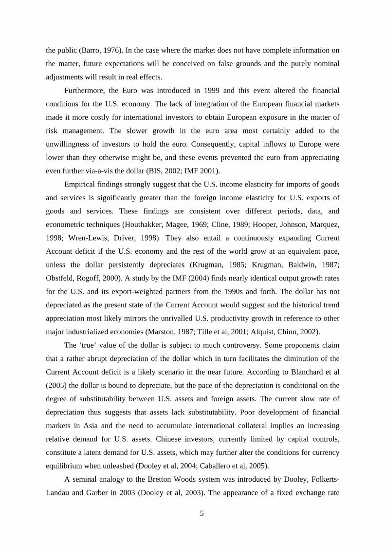
3.2.3.4 The Federal Reserve’s Discount Rate (DWPCR)

The discount rate affects liquidity, inflation, interest rates and consequentially real

economic activity (Romer, 2006). The Federal Reserve’s Discount rate thus affects the

probability of a recession and it could be useful with an explanatory variable accounting for

the effects of the discount rate. The Board of Governors of the Federal Reserve System

replaced the discount rate with the Discount Window Primary Credit Rate (DWPCR) on

January 9 2003 (Federal Reserve Release, 2002). The former discount rate was a below-

market rate whereas the DWPCR is a market-based rate. Therefore it will not be possible to

create a time series from 1980 to 2005 without a break and hence a bias in the data will occur.

Furthermore, the effects of the DWPCR are implicitly mirrored by the Interest Rate

Spread series (see 3.2.2.6). As the DWPCR rise, so will the interest rates on the 3 month U.S.

Treasury securities. An auxiliary regression where the Fed Discount Rate series is regressed

upon the 3 month U.S. Treasury securities series (T-bill 3 months) reveals that the two are

28

collinear from the 2R of 0.94 (Figure 3.1)11. Therefore, I will not include such an explanatory

variable.

Correlation of T-bill 3 month maturity and DWPCR

0,00%

2,00%

4,00%

6,00%

8,00%

10,00%

12,00%

14,00%

16,00%

1982:01

1985:03

1989:01

1992:03

1996:01

1999:03

2003:01

1990-03

1991-05

1992-07

1993-09

1994-11

1996-01

1997-03

1998-05

1999-07

2000-09

2001-11

2003-01

2004-03

2005-05

Fed discount rateT-bill 3 months

Figure 3.1: Correlation of the 3 month U.S. Treasury security and the Discount Window

Primary Credit Rate

11 An explanation for the rationale of the auxiliary regression is found in Chapter 4. For an exposition on

the definition and the implication of collinearity, see Hill et al (2001).

29

4 Result

The first sequence of computations is made as all explanatory variables are regressed on

the four dependent variables, respectively. The results are accounted for in Table 4.2. In the

first column entitled Model, the model that is being tested is specified. In the second column

entitled 2,ipR , the model’s measure-of-fit is accounted for. The index i represents the number of

the estimated regression. In the third and fourth column, 1γ and 2γ are accounted for through

their p-value respectively. Among the explanatory variables in the models below are the

following denotations applied (Table 4.1).

yi Dependent variable of series i.

β i Coefficient; β 1 represents an intercept.

ε Error term.

a Asset Price.

ca Current Account to GDP.

cr Domestic Credit.

i Domestic Investments.

ny NYSE.

nys NYSE STD.

sp Interest Rate Spread.

un Unemployment.

Table 4.1: Denotations of explanatory variables

Nr Model 2,ipR 1γ 2γ

1 εβββββββββ +++++++++= unspnysnyicrcaay '9

'8

'7

'6

'5

'4

'3

'2

'11 0.500 0.00 0.00

2 εβββββββββ +++++++++= unspnysnyicrcaay '9

'8

'7

'6

'5

'4

'3

'2

'12 0.571 0.22 0.23

3 εβββββββββ +++++++++= unspnysnyicrcaay '9

'8

'7

'6

'5

'4

'3

'2

'13 0.562 0.37 0.21

4 εβββββββββ +++++++++= unspnysnyicrcaay '9

'8

'7

'6

'5

'4

'3

'2

'14 0.723 0.53 0.37

Table 4.2: First sequence of computations

30

In Table 4.2 it is clear that model nr 4 is the most appropriate for forecasting recessions

with respect to the measure-of-fit. The 24,pR assumes a value of 0.723 which is equal to stating

that model nr 4 is predicting an average of 72.3% of the in-sample observations correctly.

Normality of the data is not attained in the first regression where the binary series of '1y is

defined as

⎩⎨⎧

=>=≤

=0,00,1'

1 ττ

growthrealifgrowthrealif

y .

The p-values for 1γ and 2γ do not indicate skewness nor kurtosis for the rest of the

regressions.

The next step will be to render the model even more parsimonious by re-estimating it

with less explanatory variables. A second sequence is made as the model is re-estimated

without one of the explanatory variables in every regression (Table 4.3).

Nr Model 2pR 1γ 2γ

5 εββββββββ ++++++++= unspnysnyicrcay '8

'7

'6

'5

'4

'3

'2

'14 0.724 0.59 0.34

6 εββββββββ ++++++++= unspnysnyicray '8

'7

'6

'5

'4

'3

'2

'14 0.724 0.73 0.35

7 εββββββββ ++++++++= unspnysnyicaay '8

'7

'6

'5

'4

'3

'2

'14 0.685 0.17 0.20

8 εββββββββ ++++++++= unspnysnycrcaay '8

'7

'6

'5

'4

'3

'2

'14 0.649 0.63 0.52

9 εββββββββ ++++++++= unspnysicrcaay '8

'7

'6

'5

'4

'3

'2

'14 0.724 0.53 0.37

10 εββββββββ ++++++++= unspnyicrcaay '8

'7

'6

'5

'4

'3

'2

'14 0.756 0.99 0.50

11 εββββββββ ++++++++= unnysnyicrcaay '8

'7

'6

'5

'4

'3

'2

'14 0.649 0.96 0.05

12 εββββββββ ++++++++= spnysnyicrcaay '8

'7

'6

'5

'4

'3

'2

'14 0.712 0.49 0.37

Table 4.3: Second sequence of computations

In the second sequence (Table 4.3), model nr 10 receives the highest value of 2pR . The

210,pR of 0.756 is higher than 2

4,pR . This implies that the model improves its in-sample

forecasting capability without the NYSE STD variable. A possible explanation for such

31

results may be that the NYSE STD series suffers from heteroskedasticity, and consequently

normality of the data is lower than otherwise. The p-values of 1γ and 2γ also receive even

more satisfactory values with respect to normality when the NYSE STD variable is excluded

than when included.

A third sequence is made as model nr 10 is re-estimated without one of the explanatory

variables in each regression (Table 4.4).

Nr Model 2pR 1γ 2γ

13 εβββββββ +++++++= unspnyicrcay '7

'6

'5

'4

'3

'2

'14 0.758 0.75 0.54

14 εβββββββ +++++++= unspnyicray '7

'6

'5

'4

'3

'2

'14 0.725 0.83 0.51

15 εβββββββ +++++++= unspnyicaay '7

'6

'5

'4

'3

'2

'14 0.682 0.17 0.18

16 εβββββββ +++++++= unspnycrcaay '7

'6

'5

'4

'3

'2

'14 0.636 0.93 0.53

17 εβββββββ +++++++= unspicrcaay '7

'6

'5

'4

'3

'2

'14 0.756 0.92 0.51

18 εβββββββ +++++++= unnyicrcaay '7

'6

'5

'4

'3

'2

'14 0.648 0.73 0.12

19 εβββββββ +++++++= spnyicrcaay '7

'6

'5

'4

'3

'2

'14 0.756 0.98 0.51

Table 4.4: Third sequence of computations

In the third sequence (Table 4.4), model nr 13 receives the highest value of measure-of-

fit, as the Asset Price variable is excluded. The 213,pR of 0.758 is higher than the 2

10,pR of

previously estimated model nr 10. Through the exclusion of Asset Price variable, the new

model receives an even higher capability of forecasting in-sample observations. Model nr 17

and nr 19, respectively estimated without the NYSE variable and the Unemployment variable,

also receive high values of measure-of-fit. A fourth sequence is made as model nr 13 is re-

estimated without one of the explanatory variables in every regression (Table 4.5).

32

Nr Model 2pR 1γ 2γ

20 εββββββ ++++++= unspnyicry '6

'5

'4

'3

'2

'14 0.748 0.65 0.51

21 εββββββ ++++++= unspnyicay '6

'5

'4

'3

'2

'14 0.605 0.08 0.05

22 εββββββ ++++++= unspnycrcay '6

'5

'4

'3

'2

'14 0.649 0.96 0.60

23 εββββββ ++++++= unspicrcay '6

'5

'4

'3

'2

'14 0.758 0.78 0.61

24 εββββββ ++++++= unnyicrcay '6

'5

'4

'3

'2

'14 0.663 0.40 0.42

25 εββββββ ++++++= spnyicrcay '6

'5

'4

'3

'2

'14 0.769 0.76 0.54

Table 4.5: Fourth sequence of computations

In the fourth sequence (Table 4.5), model nr 25 receives the highest value of 2pR . The

remaining explanatory variables are the Current Account to GDP variable, the Domestic

Credit variable, the Domestic Investments variable, the NYSE and the Interest Rate Spread

variable. The 225,pR of 0.769 is higher than the previously estimated 2

13,pR of 0.758, and further

improvement of the models forecasting capability has been achieved.

Model nr 21 testifies of low p-values for 1γ and 2γ , such that normality is rejected at

the significance level of 1.0=α . A possible explanation for the lack of normality is that the

Domestic Credit variable contains vital information for the validity and the forecasting

capability of the model. The probability of recession is thus significantly dependent on the

level of domestic consumer credit liability of U.S. households.

A fifth sequence is made as model nr 25 is re-estimated without one of the explanatory

variables in every regression (Table 4.6).

Nr Model 2pR 1γ 2γ

26 εβββββ +++++= spnyicry '5

'4

'3

'2

'14 0.740 0.67 0.50

27 εβββββ +++++= spnyicay '5

'4

'3

'2

'14 0.615 0.13 0.08

28 εβββββ +++++= spnycrcay '5

'4

'3

'2

'14 0.670 0.91 0.95

29 εβββββ +++++= spicrcay '5

'4

'3

'2

'14 0.758 0.81 0.63

30 εβββββ +++++= nyicrcay '5

'4

'3

'2

'14 0.620 0.44 0.47

Table 4.6: Fifth sequence of computations

33

Table 4.6 reveals that no further elimination of explanatory variables will improve the

measure-of-fit for the model, the best regression being nr 29 with a 229,pR equal to a value of

0.758 which is inferior to 225,pR of 0.769. Model nr 27 corroborates the previous finding that

the Domestic Credit variable holds information vital to the model’s validity and forecasting

capability.

4.1 The Final Model

The model with the best measure of fit includes the explanatory variables the Current

Account to GDP variable, the Domestic Credit variable, the Domestic Investments variable,

the NYSE and the Interest Rate Spread variable. It achieves a measure-of-fit of 0.769 (Table

4.7) and the normality of the data cannot be rejected at any conventional level of significance

based on the p-values of 1γ and 2γ .

Variable Coefficient Std. Error P-value '

1β -54.35 21.91 0.01

ca 0.37 0.68 0.58

cr 9.47 2.44 0.00

i -11.35 3.61 0.00

ny 0.60 1.21 0.62

sp -0.35 0.14 0.01

1γ 0.76 2γ 0.54

Table 4.7: The final model

The p-values of the variables Current Account to GDP and NYSE imply that they are

not statistically significant as the null hypothesis cannot be rejected at any conventional level

of significance. When estimating the model without these variables the measure-of-fit

decreases to 0.735; the small deterioration in measure-of-fit supports the low significance of

the variables. In a forecasting scenario it may be easier to do without these variables as fewer

34

variables suggest fewer factors to take into account, but I will not alter the model at the

expense of worsening the forecasting capability.

Three of the explanatory variables suffer from collinearity. An auxiliary linear

regression where the Domestic Credit is regressed upon Domestic Investments and NYSE

with an intercept reveals from the 2R of 0.96 that they are collinear. If the 2R from such

auxiliary regression assumes a value above 0.80, it implies that a large portion of the variation

in the dependent variable is explained by the variation in the explanatory variables (Hill et al,

2001).

The heteroskedasticity test reveals from the p-value of 0.61 that the final model does not

suffer from heteroskedasticity. I let the squared Current Account to GDP represents the

variable zi in the auxiliary regression since it naturally has a very small intercept and the test

statistic is thus Chi-squared of one degree of freedom. The p-value of 0.61 implies that the

null hypothesis of homoskedasticity cannot be rejected at any conventional level of

significance. Along with the previous assumption of normality which has not been rejected

from previous tests of significance, no econometrical evidence of biasness at specified levels

can be sustained and it can be informative to study the separate coefficients and their marginal

effects.

4.1.1 Marginal Effects The marginal effects have to be computed separately. As marginal effects are smaller

when located at the tails of the probability density function { }...f the marginal effect will vary

across the time series according to the value of ix'β . In order to compute a constant marginal

effect, I will let the mean of computed marginal effects according to the expression

( ) iixf ββ ˆ'ˆ− represent the marginal effect of each variable (Table 4.8, column M. E. Mean a).

An alternative approach for computing marginal effects is to take the mean of all xi and then

compute the marginal effects according to the expression ( ) iixf ββ ˆ'ˆ− (Table 4.8, column M.

E. Mean b). The different approaches yield not too differentiated values.

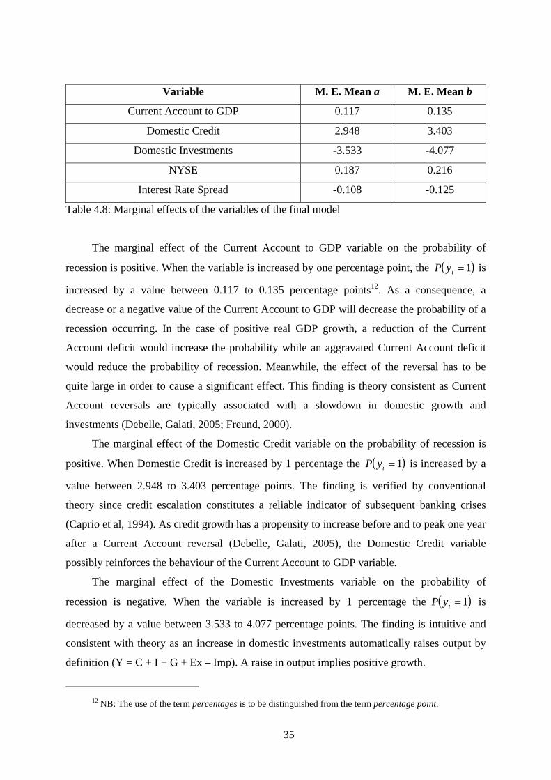
35

Variable M. E. Mean a M. E. Mean b

Current Account to GDP 0.117 0.135

Domestic Credit 2.948 3.403

Domestic Investments -3.533 -4.077

NYSE 0.187 0.216

Interest Rate Spread -0.108 -0.125

Table 4.8: Marginal effects of the variables of the final model

The marginal effect of the Current Account to GDP variable on the probability of

recession is positive. When the variable is increased by one percentage point, the ( )1=iyP is

increased by a value between 0.117 to 0.135 percentage points12. As a consequence, a

decrease or a negative value of the Current Account to GDP will decrease the probability of a

recession occurring. In the case of positive real GDP growth, a reduction of the Current

Account deficit would increase the probability while an aggravated Current Account deficit

would reduce the probability of recession. Meanwhile, the effect of the reversal has to be

quite large in order to cause a significant effect. This finding is theory consistent as Current

Account reversals are typically associated with a slowdown in domestic growth and

investments (Debelle, Galati, 2005; Freund, 2000).

The marginal effect of the Domestic Credit variable on the probability of recession is

positive. When Domestic Credit is increased by 1 percentage the ( )1=iyP is increased by a

value between 2.948 to 3.403 percentage points. The finding is verified by conventional

theory since credit escalation constitutes a reliable indicator of subsequent banking crises

(Caprio et al, 1994). As credit growth has a propensity to increase before and to peak one year

after a Current Account reversal (Debelle, Galati, 2005), the Domestic Credit variable

possibly reinforces the behaviour of the Current Account to GDP variable.

The marginal effect of the Domestic Investments variable on the probability of

recession is negative. When the variable is increased by 1 percentage the ( )1=iyP is

decreased by a value between 3.533 to 4.077 percentage points. The finding is intuitive and

consistent with theory as an increase in domestic investments automatically raises output by

definition (Y = C + I + G + Ex – Imp). A raise in output implies positive growth.

12 NB: The use of the term percentages is to be distinguished from the term percentage point.

36

The marginal effect of the NYSE variable on the probability of recession is positive.

When the variable is increased by 1 percentage the ( )1=iyP is increased by a value between

0.187 to 0.216 percentage points. This finding is somewhat dubious with respect to

conventional theory as, in the words of Estrella and Mishkin (1998, p. 49), “Finance theory

suggests that stock prices may be interpreted as expected present values of future dividend

streams.”. High future dividend streams condition high future revenues, and these future

revenues condition high future consumption which could be the result of real growth in

domestic output. In such case, an increase in the NYSE variable should yield a decrease in the

( )1=iyP , equivalent to a decrease of the probability of a recession occurring, given that real

growth facilitates the occurrence of high future dividend streams.

An alternative approach would be that growth in the NYSE variable indicates an

elevated presence of speculative bubbles that might result in a stock market crash. A stock

market crash is empirically considered to be an element in a financial crisis and a possible

adhering recession (Mishkin, 1996b). In such case, the finding is correct. These contradictory

interpretations might be an explanation for the low significance of the variable. Nevertheless,

the three variables Domestic Credit Log Level, Domestic Investments and NYSE are closely

correlated, which implies that they should be evaluated together.

The marginal effect of the Interest Rate Spread variable on the probability of recession

is negative which is equivalent of stating that when the variable is increased by one

percentage point the ( )1=iyP is decreased by a value between 10.8 to 12.5 percentage

points. Conversely, a decrease of the spread translates into an increase in the probability of a

recession occurring. The result is consistent with previous research as an increase in the short

rate is likely to flatten the yield curve and the interest rate spread and to reduce real growth in

the near term (Estrella, Mishkin, 1998). The final model is thus fairly consistent with

conventional theory. The fitted probabilities of the model are depicted in figure 4.1.

37

Fitted Probabilities

0,0

0,1

0,2

0,3

0,4

0,5

0,6

0,7

0,8

0,9

1,0

198219831984198519861987198819891990199119921993199419951996199719981999200020012002200320042005

Pyŷ

Figure 4.1: In-sample prediction by final model. Actual series of dependent variable y4 (y),

and fitted probabilities (ŷ).

38

5 Analysis

The analysis will consist of various scenarios in which the future probability of

recession is evaluated under various circumstances within the framework of the model. The

premier part of the analysis will consist of a partial analysis of the various variables’ impact

on the probability of recession. The purpose is to establish by what minimum amount a

specific variable must change, ceteris paribus, in order to provoke a recession. The changes

will be determined given that the rest of the variables remain constant. The three collinear

variables Domestic Investments Log Level, Domestic Credit and NYSE will also be treated

jointly due to their high collinearity. The model cannot credibly simulate the probability in a

scenario where the three variables do not coincide due to their correlation. Of course,

exceptions can be made from the rule, such as a stock market crash for instance where the

NYSE decreases separately along the lines of a couple of additional percentage points.

The second part will try to establish a parallel to the Current Account reversal in 1987.

It was at the time the largest Current Account deficit observed in the history of the U.S., and

many opinions were voiced on the future of the U.S. economy13. The purpose of the scenario

is to establish the probability of recession if historic events were come to pass.

The third part will consist of a speculative scenario in which the explanatory variables

follow a predetermined trend motivated by inflationary pressures. I will assume a causal chain

of events – although the model does not reflect causality – in order to permit structure in the

process of analysing and exogenously determined trends for the Current Account to GDP and

the Interest Rate Spread. The model statistically relates the appearance of certain events to the

probability of a recession, which in this context is defined as real GDP growth below its mean

for the period 1982 to 2005. The assumption of causality should therefore be considered in

this light. It is not positively established whether a change in the explanatory variables

engenders a change in the dependent variable or vice versa, but it is established that they

coincide. The assumption of causality remains inferior to the actual correlation of changes.

13 See Marris (1985) for an exposition on contemporary aspects and implications of the 1987 Current

Account deficit.

39

5.1 Partial Analysis

The partial analysis of each variable will be elaborated according to the condition that

the probability of recession must be superior to 50% after a period of 12 quarters due to the

change in one variable, while the other variables remain constant. The quarterly rate of

change in a variable will be constant for the period. The result will be computed through the

use of an iterative process, and is consequently not solved for analytically. The probability of

a recession in the last in-sample observation, 2005q4, is estimated to be approximately 0.18

which indicates that the model does not forecast an impending risk of recession.

In the case where the Current Account to GDP variable assumes an increase of 0.2

percentage points per quarter, the result will be a probability of recession superior to 0.5 in

2008q4. For the period 2005q4 (the last in-sample observation) to 2008q4, the Current

Account to GDP increases from -1.78% to 0.63%14, and the total change in Current Account

to GDP is 2.4 percentage points. Bear in mind that recession in the particular context implies

a decrease in real GDP growth below its mean. An increment of 0.2 percentage points of the

Current Account to GDP will thus engender a probability of a slight stagnation of the growth

rate; not a probability of an imminent hard landing. A comparison of the previous Current

Account reversal in 1987 reveals that the mean of the increment of the period 1986q4 to

1989q3 is approximately 0.03 percentage points, which is far from the required increment of

0.2 percentage points under these circumstances although the comparison is somewhat

inequitable.0

For an increase in the Current Account to GDP variable to take place, an increase of the

numerator (Current Account) or a decrease of the denominator (GDP), or both, is needed. It

implies that if the variable increases through a decrease in GDP, the increase in probability of

recession is self-evident and clearly endogenous. On the other hand, if the variable increases

through a positive increase in the Current Account (the deficit turns into a surplus) while GDP

continues along its mean, the amount of change in the Current Account has to be substantially

large. A hypothetical increase has to be equivalent to a sum of 1.1 trillion dollars (base year

2000) for the period 2006q1 to 2008q4 for the probability of a recession to surmount 50%.

This figure can be compared to the Current Account deficit of 2005. In 2005q4 the Current

Account deficit was 226.8 billion dollars (seasonally unadjusted) and it added up to 804.9

14 The values and the change may seem low but keep in mind that the Current Account numerator is

computed on a quarterly basis whereas the GDP denominator is computed on an annual basis.

40

billion dollars for the year 2005 (Bureau of Economic Analysis, 2006). The slower the

turnaround of the Current Account deficit the larger the accumulated sum.

For the probability of recession to surpass 0.5 in the end of 2008q4, the three variables

Domestic Credit Log Level, Domestic Investments and NYSE will have to assume a decrease

of 5.95 percentage points per quarter, and they assume identical decreases due to their high

correlation. For the NYSE series, there are periods of occasional observations of larger

decreases, especially in 2000q4 to 2003q1, whereas the other series do not exhibit periods of

such decreases more than for a rare observation or two. From a historical point of view the

decrease is improbable. For the period 2005q4 to 2008q4, the decrease accumulates to 979

billion dollars in the Domestic Credit and 1.2 trillion dollars in the Domestic Investments. The

changes are equivalent to a log decrease of 0.72. The change in the NYSE is equal to 3871

points.

If the Interest Rate Spread variable takes on a decrease of 0.22 percentage points per

quarter accumulating to a total negative change of 2.62 percentage points, the probability of

recession surpasses 0.5 in 2008q4. Large decreases of the Interest Rate Spread has been

observed in the pass: a total decrease of 1.86 percentage points in 1985q2 to 1986q2; a total

decrease of 2.52 percentage points in 1988q3 to 1989q3; a total decrease of 2.51 percentage

points in 1994q3 to 1995q4; a total decrease of 1.72 percentage points in 1999q4 to 2000q4

and a total decrease of 2.92 percentage points in 2004q3 to 2005q4. Based on historical

observations, the scenario is not unlikely to occur in the future although perhaps not under

these particular assumptions. The last period of descending Interest Rate Spread, 2004q3 to

2005q4, indicates that the probability of recession has risen rapidly and that lower future

growth has become more likely.

Mutual for the different analyses are that quarterly calculations add up to a different

amount under alternative assumptions. It is not until after the decisive change in trajectory has

taken place of a variable and continued for some time that the imminent probability of

recession occurs. It implies that the variables may vary considerably without provoking

noteworthy impact on the probability of recession.

41

5.2 Parallel to the Current Account Reversal in 1987

The U.S. experienced a Current Account reversal in 1987 combined with a stock market

correction October 19 known as the Black Monday. During this period real GDP growth never

went into a recession, defined as negative growth for two consecutive quarters, nor did it stay

below its mean for more than a couple of scattered quarters after the reversal even though the

worries for a severe impact of a large Current Account deficit were as large then as they are

today.

The values for each variable in the period 2006q1 to 2008q4 have been derived from

data of the period 1986q4 to 1989q3. The forecasted values assume the same relative changes

as the values exhibited in the period 1986q4 to 1989q3 and the forecasted values can be

observed in figure 5.2.1 to 5.2.6. For the period 2006q1 to 2008q4 the increase in Current

Account to GDP is equivalent to 0.4 percentage points, the increase in Domestic Investments

is 0.063 log units which is also equivalent to 6.3 %, Domestic Credit increases by 0.089 log

units and NYSE increases by 0.316 log units. The stock market correction is reflected by a

decrease of 0.224 log units of the NYSE in 2007q1.

Current Account to GDP

-2,0%

-1,8%

-1,6%

-1,4%

-1,2%

-1,0%

-0,8%

-0,6%

-0,4%

-0,2%

0,0% 1986:04

1987:01

1987:02

1987:03

1987:04

1988:01

1988:02

1988:03

1988:04

1989:01

1989:02

1989:03

1986q3-1989q4

2005q1-2008q4Interest Rate Spread

-1,5%

-1,0%

-0,5%

0,0%

0,5%

1,0%

1,5%

2,0%

2,5%

3,0%

3,5%

1986:04

1987:01

1987:02

1987:03

1987:04

1988:01

1988:02

1988:03

1988:04

1989:01

1989:02

1989:03

1984q3-1989q4

2005q1-2008q4

Figure 5.2.1: Current Account to GDP – 1987

Current Account reversal

Figure 5.2.2: Interest Rate Spread – 1987

Current Account reversal

42

NYSE

6,5

7,0

7,5

8,0

8,5

9,0

9,5

1986:04

1987:01

1987:02

1987:03

1987:04

1988:01

1988:02

1988:03

1988:04

1989:01

1989:02

1989:03

1986q3-1989q4

2005q1-2008q4Domestic Credit

13,6

13,8

14,0

14,2

14,4

14,6

14,8

1986:04

1987:01

1987:02

1987:03

1987:04

1988:01

1988:02

1988:03

1988:04

1989:01

1989:02

1989:031986q3-1989q4

2005q1-2008q4

Figure 5.2.3: NYSE – 1987 Current Account

reversal

Figure 5.2.4: Domestic Credit – 1987 Current

Account reversal

Domestic Investments

6,7

6,9

7,1

7,3

7,5

7,7

7,9

1986:04

1987:01

1987:02

1987:03

1987:04

1988:01

1988:02

1988:03

1988:04

1989:01

1989:02

1989:03

1986q3-1989q4

2005q1-2008q4Forecasted Probabilities

0,0

0,1

0,2

0,3

0,4

0,5

0,6

0,7

0,8

0,9

1,0

1986:04

1987:01

1987:02

1987:03

1987:04

1988:01

1988:02

1988:03

1988:04

1989:01

1989:02

1989:03

1986q3-1989q4

2005q1-2008q4

Figure 5.2.5: Domestic Investments – 1987

Current Account reversal

Figure 5.2.6: Fitted Probabilities – 1987

Current Account reversal

The probability of a recession in the last in-sample observation, 2005q4, is estimated to

be approximately 0.18. The stock market correction does not seem to have a severe impact on

the probability of recession. The NYSE series has a negative marginal effect on the

probability of recession in the case of a reduction. Hence, the decrease in NYSE of 0.224 log

units in 2007q1 does not correlate to an increase in probability of recession given the

development of the other variables. From 2007q4 to 2008q4 the probability of recession

surges from 0.23 to 0.55, and thus a predicted recession does not occur until the last quarter of

2008.

A comparison of probabilities of recession reveals that the mean of the calculated

differences of probabilities from the two periods is approximately 31% lower in 2006q1 to

2008q4 than in 1986q4 to 1989q3. The lower mean may suggest, from an econometrical point

of view, that the rather large Current Account deficit operates in favour of the U.S. economy

43

to a greater extent than in the past in spite of the Interest Rate Spread which assumes an

unusually small (negative) value. In more general terms, the lower mean may suggest that the

U.S. economy rests on a more solid ground than in the past. As financial- and goods-markets

become globally integrated the result will probably be higher growth. The amount of U.S.

trade, defined as [Imports + Exports, nominal values] (Bureau of Economic Analysis, 2006)

has been growing with a mean of 1.84% per quarter for the period 1982 to 2005. However,

the mean of 1.79% from the period 1982 to 1993 is lower than the mean of 1.86% from the

period 1994-2005, which could reflect the entrance of new emerging markets in larger parts of

Asia on the global arena of trade.

5.3 Inflationary Pressures

The inflationary aspect is motivated by the general importance of monetary policy for

economic growth and the fact that inflation is a factor which is mainly determined by

domestic macroeconomic indicators; domestic in the sense that it arises from positive

domestic demand conditions and higher domestic wages. In the case where heavy exports

exert upward pressure on domestic inflation through an increase in demand - a foreign factor

– such pressure is relatively feeble in comparison to inflation due to an equivalent increase in

domestic consumption. Consumption is approximately seven times as large as exports in the

measure of GDP from the year 1982 to 2005 (Bureau of Economic Analysis, 2006).

The main complication when choosing the development of domestic inflation as a key

factor in a future speculative scenario is that inflation is complex and subdued to the influence

of a multitude of factors. Future expectations, the technological evolution, the stickiness of

nominal prices and the wage setting process, to mention some factors, all play a part in how

inflation arises (Romer, 2006). It will not be possible to assess the effects of all factors and the

key argument when basing a future scenario on inflationary pressure remains that it is chiefly

a domestic phenomenon.

Imported inflation exerts a downward pressure on nominal output growth and domestic

inflation. Through the definition of GDP (Y = C + I + G + Ex - Imp) it is easily observed that

an increase in foreign price levels will cause the immediate value of imports to rise and GDP

to decline in the short term. In reference to previous mentioned scenarios, an increase in the

price of oil may instigate an aggregate supply shock which might turn into domestic inflation.

The oil dependent firms chose to pass the increase in cost to their customers and ultimately

the consumers by raising prices (Romer, 2006).

44

The scenario in the previous subchapter 5.2 shed light on a possible development of the

probability of recession in the case of a Current Account reversal and a heavily deteriorating

interest rate spread; two factors working for an increase of the probability of recession. In this

scenario, the assumptions will be slightly different. Global investors maintain their

expectations on sufficient returns from the U.S. economy, thus continuing to extend the

access to foreign capital at a previous rate. They might do this for a variety of reasons, but I

will assume that the motive is conceived along the lines of subchapter 2.1. Higher real growth

of the U.S. economy vis-à-vis its competitors, perceived higher risk in the rest of the world

and similar incentives will have investors turning their eyes towards the U.S. Consequently,

capital inflows to the U.S. will continue to be relatively elevated and I will assume that the

negative Current Account to GDP will continue to deepen at the same rate as it has done for

the period 2003q1 to 2005q4.

On the domestic scene, the Board of Governors of the Federal Reserve System (from

now on referred to as the Fed) continue the raise of the DWPCR according to the mean of the

rate of 2003q1 to 2005q4 (0.25 percentage points per quarter) for another 4 quarters before

arriving at a plateau for which the DWPCR remains constant. The behaviour is meant to

reflect previous raises in the periods 1994q4 to 1996q4 and 1987q2 to1989q2 which have

both arrived at a plateau and remained constant for some time. The steep and massive raise

may be a strong assumption to make for the evolution of the DWPCR. The raise for the period

2004q2 to 2008q4 is equivalent to 3.96 percentage point which is an unprecedented raise in

the history of the Fed. The justification for such a raise might be to counter the inflationary

effect of the inflow of capital indicated by an also unprecedented Current Account deficit, or

to counter inflationary effects from soaring oil prices. I will assume unaltered expectations in

the medium term and the last observation of the rate of the 10 year maturity U.S. Treasury

security will function as a guideline value for 2005q1 to 2008q4 when computing the Interest

Rate Spread. The value of the 3 month maturity U.S. Treasury security will be given by the

DWPCR since they correlate closely.

The three variables Domestic investments, Domestic Credit and NYSE will react as a

result of the raise in DWPCR. To facilitate the forecasting of the variables, I have computed

three linear regressions where I regress each of the variables upon the Primary Discount Rate

and the Current Account to GDP (Table 5.3.1). The p-values for all coefficients are zero.

45

Regression R2

Crediti = 14,16 - 0,07*DWPCRi - 0,35*Current Account to GDPi 0.82

Invi = 7,37 - 0,06*DWPCRi - 0,34*Current Account to GDPi 0.81

NYSEi = 8,65 - 0,16*DWPCRi - 0,44*Current Account to GDPi 0.73

Table 5.3.1

The regressions in Table 5.3.1 are biased due to endogeneity, but the purpose is not to

analyze the results; they are entirely meant to provide assistance in the forecasting of the

variables. The endogeneity of the regression may be subject to discussion, but I would like to

assume exogenous explanatory variables for the sake of argument. To the extent that the

dependent variables affect the explanatory variables, it is rather the expected future values of

the dependent variables that are conditioning the evolution of the present values of the

explanatory variables. The DWPCR for instance is managed in accordance with future

expectations on inflation, unemployment or real and nominal output (Romer, 2006). The

Current Account to GDP is by definition endogenous with respect to Domestic Investments,

but the endogeneity is less apparent with respect to Domestic Credit and NYSE.

The forecasted values are generated by calculating the forecasted values of each

variable from the assumed evolution made earlier of the DWPCR and the Current Account to

GDP from the period 2005q1 to 2008q4. The relative changes of the period are then applied to

the real series with the purpose of producing a reasonable forecast of Domestic Credit,

Domestic Investments and NYSE. The results are depicted in figure 5.3.1 to 5.3.6.

Under these circumstances it is possible to compare computed probabilities of the 1987

Current Account reversal from the model at hand along with linearly generated forecasts of

Domestic Investments, Domestic Credit and NYSE (Model 5.3), with the probabilities

generated by the model from subchapter 5.2 (Model 5.2). In Model 5.3 forecasted values are

derived from historic data for the Current Account to GDP as well as the Interest Rate Spread,

while Domestic Investment, Domestic Credit and NYSE are generated by the equations in

Table 5.3.1. In Model 5.2 all forecasted values are derived from historic data (figure 5.3.7).

They appear to predict the historic event similarly, apart from the end observations, and an

auxiliary regression reveals by the R2 of 0.77 that they are closely correlated, in spite of the

meagre sample. The discrepancy of the probabilities from the two models has a mean of

0.0334 and a standard deviation of 0.0713.

46

Current Account to GDP

-3,0%

-2,5%

-2,0%

-1,5%

-1,0%

-0,5%

0,0% 2000

2001

2002

2003

2004

2005

2006

2007

2008

2000q1-2008q4 Interest Rate Spread

-2,0%

-1,0%

0,0%

1,0%

2,0%

3,0%

4,0%

2000

2001

2002

2003

2004

2005

2006

2007

20082000q1-2008q4

Figure 5.3.1: Current Account to GDP –

Inflationary pressures

Figure 5.3.2: Interest Rate Spread –

Inflationary pressures

NYSE

8,4

8,5

8,6

8,7

8,8

8,9

9,0

9,1

9,2

2000

2001

2002

2003

2004

2005

2006

2007

2008

2000q1-2008q4 Domestic Credit

14,20

14,25

14,30

14,35

14,40

14,45

14,50

14,55

14,60

14,65

14,70

2000

2001

2002

2003

2004

2005

2006

2007

2008

2000q1-2008q4

Figure 5.3.3: NYSE – Inflationary pressures Figure 5.3.4: Domestic Credit – Inflationary

pressures

Domestic Investments

7,4

7,5

7,6

7,7

7,8

7,9

8,0

2000

2001

2002

2003

2004

2005

2006

2007

2008

2000q1-2008q4 Forecasted Probabilities

0,0

0,1

0,2

0,3

0,4

0,5

0,6

0,7

0,8

0,9

1,0

2000

2001

2002

2003

2004

2005

2006

2007

2008

2000q1-2008q4

Figure 5.3.5: Domestic Investments –

Inflationary pressures

Figure 5.3.6: Forecasted Probabilities –

Inflationary pressures

47

Forecasted Probabilities

0,0

0,1

0,2

0,3

0,4

0,5

0,6

0,7

0,8

0,9

1,0

2006:01

2006:02

2006:03

2006:04

2007:01

2007:02

2007:03

2007:04

2008:01

2008:02

2008:03

2008:04

5.2 1987 Parallel5.3 Inflationary Impact

Figure 5.3.7: Comparison of forecasted probabilities (model 5.3) and computed

probabilities (model 5.2) on the 1987 Current Account reversal.

Forecasted probabilities of recession reveal that no moderate increase in inflation and

subsequent raises of the DWPCR will pose an imminent threat to the U.S. economy as long as

the U.S. retain its global credibility as a ‘good investment’. The probability will peak in

2006q4 with a value of 0.34, and fade from thereon as the Current Account to GDP continues

to deepen. In fact, the robustness of the economy is quite impressive under these assumptions.

The Fed would have to effectuate a quarterly increase of 0.27 percentage points of the

DWPCR for the following 12 quarters for the probability to surpass the 0.5 threshold. The

result would be an astounding Interest Rate Spread of -3.74 percentages, unprecedented in the

history of the U.S., and therefore I will have to conclude that the real conundrum is the future

development of the Current Account to GDP.

48

6 Conclusion

Recent events, such as the deteriorating Interest Rate Spread, indicate that the U.S.

economy has embarked on some sort of adaptation to lowered expectations on future real

growth, although the prospect of a recession as defined by conventional standards, or ‘hard

landing’, seems less likely in the light of the various scenarios. The probability of a financial

crisis however cannot be explored within these frameworks. The U.S. economy simply

appears to be sturdier nowadays than 20 years ago, even if the solid inflow of capital on

which the U.S. is resting is conditioned upon the expectations as being a sound investment to

foreign investors. A possible explanation for the seemingly robust U.S. economy might be

given by the new emerging markets in Asia, which emerged after the dissolution of the Soviet

Union. As they become increasingly open to foreign- and U.S. capital especially, their fresh

surge in growth generates capital transfers in form of returns on U.S. held regional assets

which in turn favour U.S. real growth. Such a state of affairs could be the case where

comparative advantages of capital and labour are exploited in their full effect, according to the

well-known principles initially presented by Adam Smith (1776).

The threat of heavy domestic inflationary pressures will not provoke a significant

increase in the probability of recession based on the predictions of the model. Needless to say,

these heavy inflationary pressures are assumed to be countered by the Fed. If such events

were to pass, as long as the Current Account deficit continues to widen the probability of

recession will not take off. These judgements are of course clouded by the out-of-sample

characteristic of the model, but they still provide a notion of what to expect in the future.

For a Current Account reversal to pose an impending threat to the U.S. economy it has

to be not only large but also swift. A moderate reversal of the Current Account deficit, along

the lines of the reversal in 1987, will increase the probability of real growth below its mean

but only after some time; the probability that the specific quarter will be a recession as

defined in model 5.2 does not appear until 2008q4. Evidently, these aspects include the hardly

predictable real exchange rate. Conventional theory suggests that a real depreciation

facilitates the upholding of trade balance in the case of a Current Account deficit by making

domestic goods more competitive, but to illuminate the complexity of the matter I use the

words of Olivier Blanchard (2003, p. 409): “But just the opposite happened to the U.S. real

exchange rate in the late 1990s: The United States experienced a real appreciation, not a real

depreciation.”. Various reasons thereof have been accounted for in chapter 2, but the incident

per se reflects an increase in the foreign demand of U.S. assets. If the U.S. economy, robust as

49

it seems under previous assumptions, does not suffer an elevated risk of recession due to its

domestic affairs, it may suffer an elevated risk of recession due to its relations with foreign

capital. The foreign demand of U.S. assets might thus be, through the Current Account

channel and the NIIP, correlated to the probability of recession. If demand of U.S. assets were

to seize there would probably be implications for the United States.

50

7 Further Research

Certain questions remain unanswered. The timing and the pace of a reversal of the

Current Account deficit has not been forecasted because it depends on difficultly assessed

foreign factors such as the political agenda in greater parts of Asia. It also comprises an

element in the forecasting of the demand of U.S. assets, which in turn depends on the value of

the dollar vis-à-vis other currencies. The future value of the dollar and its effect on the

Current Account and the NIIP is interesting and complex to estimate as global integration

evolves over time. Much of U.S. foreign liabilities are denominated in U.S. dollars, whereas

U.S. foreign assets are frequently denominated in foreign currencies. A depreciation of the

dollar would leave the value of the liabilities unchanged but it would boost the US dollar

value of foreign assets. Consequently a depreciation of the dollar would reduce the value of

U.S. net foreign liabilities, and improve the NIIP (Debelle, Galati, 2005). Is it reasonable to

assume that a similar improvement of the NIIP could encourage foreign investors to continue

acquiring U.S. assets, and if so, to what extent?

An alternative approach when studying the foreign held U.S. assets and the probability

of recession is to scrutiny the incentives for upholding the value of the dollar. In the case of

the U.S. – China nexus, this approach can become quite interesting. By revaluating the

Renminbi, the Chinese authorities implicitly reduce the value of their U.S. holdings, when

denominated in Renminbi, as they are to a great extent denominated in U.S. dollars. The

appreciation of the Renminbi also reduces the competitiveness of Chinese goods in

comparison to U.S. goods, and lesser exports are to be expected. Is such an event in the

interest of the Chinese authorities?

The inflationary aspect of subchapter 5.3 and affiliated raises in the U.S. DWPCR

becomes quite remarkable when combined with additional observations from previous

research. If U.S. interest rates were to take off, the Chinese interest rates would have to rise by

an equal amount in order to retain domestic liquidity as the renminbi is committed to a fixed

parity. If the Chinese authorities would not follow up with a raise in discount rate, they would

probably engender a loss of Chinese reserves. To complete the picture, I refer to Goldstein

and Lardy (2004) who have stated that “the increase in domestic currency credit extended in

2004 will almost certainly be the second highest ever. It will take additional years of

moderating credit growth to get investment down to a sustainable level”. A raise in interest

rates would definitely cool off the Chinese economy through their large stock of domestic

credit.

51

If a large part of these loans would turn into non-performing-loans (NPL)15, or ‘bad

credit’, as roughly 40% of them did in the last Chinese credit boom in the early 1990s

(Goldstein, 2004), then the Chinese authorities could have to deal with a financial crisis as

defined by Bordo et al (2001, p. 55)16. The NPLs would also pose a serious problem for

domestic banks, possibly provoking a bank crisis. If foreign investors were to sell off their

Chinese assets en masse due to the newly emerged crisis, or to use a term of Calvo and

Mendoza (1997), act according to a herding behaviour in the absence of satisfactory

information quality, a plunge in asset prices would take place (after all, the foreign investors

acting on a market where information is scarce infer information from the actions of other

investors).

The implications for the U.S. would be transferred through two channels mainly. The

first channel is the Renminbi. A similar bank crisis could very well turn into a Chinese

currency crisis as foreign investors withdrew their assets and exchanged them for dollars.

Problems in the banking sector typically precede a currency crisis and the currency crisis

deepens the banking crisis, thus reinforcing each other (Kaminsky, Reinhart, 1999). If

Chinese reserves were depleted, the fixed exchange rate would have to be dropped, and the

Renminbi would probably depreciate as to reflect the poor state of the economy, in which

case the position of Chinese banks would be weakened further if a large share of their

liabilities were denominated in foreign currency (Mishkin, 1996a). The plunge of the

Renminbi would strengthen the U.S. dollar even further. Depending on the Marshall-Lerner

effect and the J-curve, the cost of imports would decrease up to six months to a year after the

currency crash (Blanchard, 2003 p. 406) only to increase in the medium term, whereas U.S.

exports would decrease. The effect on the U.S. real GDP would probably be negative.

The second channel consists of the U.S. held Chinese assets. The crisis in China could

transmit to the U.S. via deteriorating Chinese assets held by U.S. banks. Banking problems

tend to arise from the deterioration in asset quality possibly resulting from a collapse in real-

estate prices or increased bankruptcies in the nonfinancial sector (Kaminsky, Reinhart 1999).

A crisis is also more likely to spread between countries through the channels of income

15 A report on Chinese NPLs were emitted by Ernst & Young as a part of their annual global survey,

stating that the value of the NPLs were as high as 900 billion U.S. dollars, approximately four times the amount

admitted by official Chinese sources (McGregor, 2006), but it was later withdrawn. 16 Bordo et al (2001, p. 55): “…episodes of financial-market volatility marked by significant problems of

illiquidity and insolvency of financial-market participants and/or by official intervention to contain such

consequences”

52

effects if there is a large degree of bilateral trade. These chains of events are particularly

noticeable in open emerging market and even ones with relatively sound fundamentals are not

capable of insulating themselves from events in the rest of the world (Fratzscher, 2003).

Goldstein (1998) put forward the observation that the level of economic activity, in the wake

of a crisis for example, spread across boarders as global operators reassess their portfolios and

strategies in accordance with altered pay-offs on investments, raising the degree of financial

market co-movements. If a classical banking crisis would strike the U.S. economy, the

implications could be grave as the liquidity and the stability of the international financial

system would be in jeopardy.

This is a scenario where the chain of events has been taken very far and they might be

unlikely to occur and definitely contested but nevertheless the probability remains if ever so

slight that they may take place in which case they will have noticeable effects on the U.S.

economy and the global economy. These events are of course difficultly assessed but still they

comprise an element in the forecasting of the probability of an occurrence of a U.S. recession.

Unfortunately, it is not within the elaborated framework of the conceived probit model to

quantify the probability of such overseas events, and even less the magnitude of the effects on

the U.S. economy.

53

References

Alquist, R., Chinn, M. D., 2002. Productivity and the Euro-Dollar Exchange Rate Puzzle,

NBER Working Paper No. 8824 Akerlof, G. and P. Romer (1993). Looting: the economic underworld of bankruptcy for profit,

Brookings Papers on Economic Activity Vol. 2, pp. 1-73. Barro, R. J., 1976. Rational Expectations and the Role of Monetary Policy. Journal of

Monetary Economics 2 (January), pp. 17-26. Bernanke, B. S., Lown, C. S., 1991. The Credit Crunch. Brookings Papers on Economic

Activity, Vol. 1991, Issue 2, pp. 205-247. Bank for international settlements (BIS), 2002. Triennial Central bank survey of foreign

exchange and derivatives market activity in 2001. March. Blanchard, O., Giavazzi, F., Sa, F., 2005. The U.S. Current Account deficit and the dollar.

MIT Department of Economics Working Paper No. 05-02 Blanchard, O., 2005. Macroeconomics, 3rd edition, international edition. Prentice Hall. Bordo, M., Eichengreen, B., Klingebiel, D., Soledad Martinez-Peria, M. Financial Crises:

Lessons from the last 120 years. Economic Policy, April 2001, Printed in Great Britain, © CEPR, CES, MSH, pp. 53-82.

Borio, C., Lowe, P., 2002. Assessing the risk of banking crises. BIS Quarterly Review,

December, pp. 43-54. Boyd, J. H., Kwak, S., Smith B., 2005. The Real Output Losses Associated with Modern

Banking Crises. Journal of Money, Credit, and Banking, Vol. 37, No. 6. pp. 977-999. Caballero, R., Farhi, E., Hammour, M., 2005. Speculative growth: Hints from the U.S.

economy, MIT. Draft April 7, pp. 1-57. Calvo, G., Mendoza, E., 1996. Petty crime and cruel punishment: Lessons from the Mexican

debacle. American Economic Review Papers and Proceedings, Vol. 96, pp. 170-175. Calvo, G., Mendoza, E., 1997. Rational herd behavior and the globalization of securities

markets. Institute for Empirical Macroeconomics Discussion Paper No. 120-1, Federal Reserve Bank of Minneapolis.

Caprio, G., Atiyas, I., Hanson, J. A., 1994. Financial reform: Theory and experience. New

York: Cambridge University Press. Cline, W. R., 1989. United States external adjustments and the world economy. Washington

D.C., Institute for International Economics.

54

Congressional Budget Office, 2003. The long term budget outlook. December, Congressional Budget Office, Congress of the United States.

Cooper, R., 2001. Is the U.S. Current Account Deficit Sustainable? Will It Be Sustained?

Brookings Papers on Economic Activity, No. 1, pp. 217-26. Debelle, G., Galati, G., 2005. Current Account adjustment and capital flows. BIS working

papers 169, Monetary and Economic Department, Bank of International Settlements, pp. 1-28.

Dooley, M., Folkerts-Landau, D., Garber, P., 2003. An Essay on the Revived Bretton Woods

System. NBER Working Paper No. 9971, September. Dooley, M., Folkerts-Landau, D., Garber, P., 2004. The U.S. Current Account deficit and

economic development: Collateral for a total return swap. NBER working paper No. 10727.

Edwards, S., 2004. Thirty Years of Current Account Imbalances, Current Account Reversals,

and Sudden Stops. IMF Staff Papers 51 (Special Issue), pp. 1-49. Eichengreen, B., 2004. Global Imbalances and the Lessons of Bretton Woods. NBER

Working Paper No. 10497, May. Eichengreen, B., 2000. Taming capital flows. World Development, Vol. 28 Issue 6, pp. 1105-

1116. Eichengreen, B., Rose, A., Wyplosz, C., 1995. Exchange market mayhem: the antecedents

and aftermath of speculative attacks. Economic Policy 21, pp. 249-312. Eichengreen, B., Mussa, M., Dell'Ariccia, G., Detragiache, E., Milesi-Ferretti, G. M.,

Tweedie, A., 1998. Capital account liberalization: theoretical and practical aspects. Occasional Paper No. 172. Washington, DC: International Monetary Fund.

Estrella, A., Mishkin F.S., 1998. Predicting U.S. recessions: Financial variables as leading

indicators. The Review of Economics and Statistics, Vol. 80, pp. 45-61. Frankel, J., Rose, K. A., 1996. Exchange Rate Crises in Emerging Markets. Journal of

international Economics, Nov 1996, 41(3), pp. 352-68. Fratzscher, M., 2003. On currency crises and contagion. International Journal of Finance &

Economics, April, Vol. 8, pp. 109-129. Freund, C., 2000. Current Account adjustment in industrialized countries. International

Finance Discussion Paper 692, Board of Governors of the Federal Reserve System. Gavin, M., Hausmann, R., 1996. The roots of banking crises: the macroeconomic context.

Inter-American Development Bank, Research Department, Working Papers No. 318.

55

Goldstein M., 1998. The Asian financial crisis: causes, cures and systematic implications. Policy Analysis in International Economics, No. 55. Washington DC, Institute for International Economics, June.

Goldstein, M., 2004. Adjusting China’s Exchange Rate Policies. Revised version of the paper

presented at the International Monetary Fund's seminar on China's Foreign Exchange System, Dalian, China, May 26-27, 2004.

Goldstein, M., Lardy, N., 2004. What Kind of Landing for the Chinese Economy? Policy

Briefs in International Economics, No. PB04-7, Institute for International Economics, Washington DC, November.

Higgins, M., Klitgaard, T., 2004. Reserve Accumulation: Implications for Global Capital

Flows and Financial Markets. Current Issues in Economics and Finance, Vol.10, No. 10, September/October, Federal Reserve Bank of New York.

Hill, R. C., Griffiths, W. E., Judge, G. G., 2001. Undergraduate Econometrics, 2nd edition.

John Wiley & Sons, Inc. Hooper, P., Johnson, K., Marquez, J., 1998. Trade elasticities for G-7 countries, Federal

Reserve Board of Governors, International finance discussion papers 609. Houthakker, H. S., Magee, S. P., 1969. Income and price elasticities in world trade. Review

of economics and statistics, May, Vol. 51, pp. 111-125. International monetary Fund (IMF), 2001. Recent structural changes in European

Government securities market. International capital Markets Developments, Prospects and Key policy Issues. Washington D.C.: International Monetary Fund, pp. 99-110.

International Monetary Fund (IMF), 2002. Essays on Trade and Finance. Chap. 3 in World

Economic Outlook, September, pp. 65-107. International Monetary Fund (IMF), 2004, U.S. selected issues, Article IV United States

Consultation-Staff Report. Kaminsky, G., Reinhart, C., 1999. The twin crises: the causes of banking and balance-of-

payments problems. American Economic Review, June, Vol. 89, No. 3, pp. 473–500. Kilian, L., and Taylor, M. P., 2003. Why is it so difficult to beat the random walk forecast of

exchange rates? Journal of International Economics, May, Vol. 60, No. 1, pp. 85-107. Kindleberger, C. P., 1996. Manias, Panics, and Crashes. A History of Financial Crises. 3rd

edition, Macmillan Press Ltd, London. Kornai, J., Maskin, E., Roland, G., 2003. Understanding the Soft Budget Constraint. Journal

of Economic Literature, Vol. 41, Issue 4, pp. 1095-1136. Krugman, P. R., 1985. Is the Strong Dollar Sustainable? The U.S. Dollar--Recent

Developments, Outlook, and Policy Options, pp. 103-132. Kansas City: The Federal Reserve Bank of Kansas City.

56

Krugman, P. R., Baldwin, R. E., 1987. The Persistence of the U.S. Trade Deficit. Brookings

Papers on Economic Activity, spring, pp. 1-55. Levey, D. H., Brown, S. S., 2005. The Overstretch Myth. Foreign Affairs. New York,

Mar/Apr. Vol. 84, Issue 2, pp. 2. Lucas, R. E. Jr., 1976. Econometric Policy Evaluation: A Critique. Carnegie-Rochester

Conference Series on Public Policy, Vol. 1, pp. 19-46. Mann, C. L., 2002. Perspectives on the US Current Account deficit and sustainability. Journal

of economic perspectives, Vol. 16, No. 3, pp. 131-152. Marris, S., 1985. Deficits and the Dollar: The World Economy at Risk. Institute for

International Economics, Policy Analysis in International Economics, November. Marston, R. C., 1987. Real Exchange Rates and Productivity Growth in the United States and

Japan. Real-Financial Linkages among Open Economies, edited by Sven W. Arndtand J. David Richardson, pp. 71-96. Cambridge MA, MIT Press.

Meade, E. E., Thomas, C. P., 1993. Using external sustainability to model the dollar.

Evaluating policy regimes: New research in empirical macroeconomics. Ralph C. Bryant, Peter Hooper and Catherine L. Mann, eds. Washington D.C.: Brookings Institution, pp. 769-92.

Milesi,-Ferreti, G. M., Razin, A., 1996. Current Account Sustainability. Princeton University,

Department of economics, International Finance Section, Princeton studies in International Finance No. 81, October.

Mishkin, F. 1996a. Understanding financial crises: A developing country perspective. Annual

World Bank Conference on development economics. Washington DC: World Bank, pp. 29-62.

Mishkin, F. 1996b. Financial Crisis, NBER Reporter; Winter, 1996/7, pp. 10-12. Mulder, C., Rocha, M., 2000. The soundness of estimates of output losses in currency crises.

Unpublished manuscript, IMF. Obstfeld, M., 2004. External Adjustment. Revised version of the Bernhard Harms Lecture

delivered at the Kiel Institute for World Economics on August 27, 2004. Review of World Economics, Vol. 140 (4), pp. 541-568.

Obstfeld, M., Rogoff, K., 2000. Perspectives on OECD economic integration: implications

for U.S. Current Account adjustment. Federal Reserve Bank of Kansas City, pp. 169-208. Obstfeld, M., Rogoff, K., 2004. The Unsustainable US Current Account Position Revisited.

NBER Working Paper No. 10869. Romer, D., 2006. Advanced Macroeconomics. 3rd edition. McGraw-Hill Irwin.

57

Solow, R. M., 1957. Technical Change and the Aggregate Production Function. Review of Economics and Statistics, Vol. 39, pp. 312-320.

Tille, C., Stoffels, N., Gorbachev, O., 2001. To what extent does productivity drive the dollar?

Federal reserve Bank of New York: Current Issues in Economics and Finance. August 7:8, pp. 1-6.

Taylor, A. M. (2002). A Century of Current Account Dynamics. Journal of International

Money and Finance Vol. 21, Issue 6), pp. 725–748. Tille, C., 2003. The Impact of Exchange Rate Movements on U.S. Foreign Debt. Current

Issues in Economics and Finance (Federal Reserve Bank of New York), Vol. 9 Issue 1, pp. 1-7.

Tille, C., 2005. Financial Integration and the Wealth Effect of Exchange Rate Fluctuations.

Federal Reserve Bank of New York, New York. Staff report No. 226. Triffin, R., 1960. Gold and the Dollar Crisis. New Haven: Yale University Press. Ventura, J., 2001. A Portfolio view of the U.S. Current Account deficit. Brookings papers on

economic activity, 1, pp. 241-53. Verbeek, M., 2004. A Guide to Modern Econometrics. 2nd ed. John Wiley & Sons Ltd. Wren-Lewis, S., Driver, R. L., 1998. Real exchange rates for the year 2000. Washington

D.C., Institute for international economics, Policy analyses in international economics 54. Yuan, M., Zimmermann, C., 1999. Credit Crunch, Bank Lending and Monetary Policy: A

Model of Financial Intermediation with Heterogeneous Projects. CREFE Working papers No. 89.

58

Internet References

Smith, A., 1776. The Wealth of Nations. http://socserv2.socsci.mcmaster.ca/~econ/ugcm/3ll3/smith/wealth/index.html

Board of Governors of the Federal Reserve System (Federal Reserve). 2006.

http://www.federalreserve.gov/ Bureau of Economic Analysis, 2006. U.S. Department of Commerce.

http://www.bea.gov/ Federal Reserve Bank of Minneapolis. 2006. Gary H. Stern, June. Pursuing Effective

Economic Policy. http://www.minneapolisfed.org/pubs/region/06-06/top9.cfm

Federal Reserve Press Release, 2002, October 31.

http://www.federalreserve.gov/boarddocs/press/bcreg/2002/200210312/default.htm Marquez, J., 2000. The puzzling income elasticity of U.S. imports, Federal Reserve Board.

http://fmwww.bc.edu/RePEc/es2000/1128.pdf McGregor, R., 2006. China bad loans may reach total of $900bn. Financial Times, May 3rd.

http://www.ft.com/cms/s/337447e4-da70-11da-aa09-0000779e2340.html NYSE Group. NYSE Composite Index. 2006.

http://www.nyse.com/marketinfo/datalib/1022221393023.html#Indices Roubini, N., Setser, B., 2005. Will the Bretton Woods 2 Regime Unravel Soon? The Risk of a

Hard Landing in 2005-2006. NYU, February. http://www.stern.nyu.edu/globalmacro/BW2-Unraveling-Roubini-Setser.pdf

U.S. Department of Labor, Bureau of Labour Statistics. 2006. http://www.bls.gov/

59

Appendix A

Source reference of data

Gross Domestic Product (GDP) Bureau of Economic Analysis (2006) Table 1.1.5. Gross Domestic Product Last Revised March 30, 2006 Price Deflator Bureau of Economic Analysis (2006) Table 1.1.9. Implicit Price Deflators for Gross Domestic Product Last Revised March 30, 2006 Asset Price Federal Reserve (2006) Unique Identifier: Z1/Z1/FL152000005.Q Households and nonprofit organizations total assets asset (Seasonally Unadjusted Level) Current Account Bureau of Economic Analysis (2006) Table 1. U.S. International Transactions Earliest Year Revised on March 14, 2006 Domestic Credit Federal Reserve (2006) Unique Identifier: Z1/Z1/FL153166000.Q Households and nonprofit organizations consumer credit liability (Seasonally Unadjusted Level) Domestic Investments Bureau of Economic Analysis (2006) Table 5.1. Saving and Investment Last Revised March 30, 2006 NYSE NYSE Group (2006) Historical Data for NYSE Composite Index (Symbol NYA) Interest Rate Spread Federal Reserve (2006) Market yield on U.S. Treasury securities at 10-year constant maturity, quoted on investment basis; Unique Identifier: H15/H15/RIFLGFCY10_N.M Market yield on U.S. Treasury securities at 3-month constant maturity, quoted on investment basis; Unique Identifier: H15/H15/RIFLGFCM03_N.M

60

Unemployment Department of Labor (2006) Series Id: LNU04000000Q Unemployment Rate; 16 years and over; Not seasonally adjusted Discount Rate Federal Reserve (2006) Average Discount Rate on Loans to Member Banks Quoted on Investment Basis, Federal Reserve Bank of New York Unique Identifier: H15/discontinued/H0.RIFSRD_F02_N.M Discount Window Primary Credit Rate (DWPCR) Federal Reserve (2006) The rate charged for primary credit under amendment to the Board's Regulation A Unique Identifier: H15/H15/RIFSRP_F02_N.M