What neuroscience can teach us about data-abundant system architectures

Bruno A. Olshausen and Pentti Kanerva Redwood Center for Theoretical Neuroscience

UC Berkeley

Principles of optics govern the design of

eyes

What are the principles governing information processing in this system?

100 Mb/sec.

How to gain insight?

• Study the brain’s anatomical structure and neural response properties (neuroanatomy/physiology) !

• Study what the brain does, and how well it does it (psychophysics/behavior) !

• Formulate theories and test against neural data and performance (computational modeling)

Two key lessons so far

1. Sparse, distributed representation of sensory information

2. High-dimensional representations(‘Hyperdimensional computing’)

How do brains process image data?

(from Kersten & Yuille, 2003)

an absolute depth judgment with respectto fixation, while fine stereopsis requiresthe judgment of relative depth, i.e., com-paring depth across space; (2) the partic-ular coarse stereopsis task used requiresthe monkey to discriminate a signal innoise, while the fine task does not; (3)the range of disparities is quite different.

Chowdhury and DeAngelis (2008) repli-cate the finding that monkeys initiallytrained on coarse stereopsis show im-paired coarse depth discrimination whenmuscimol is injected into MT. Remark-ably, the same animals, after a secondround of training on fine stereopsis, areunimpaired at either fine or coarse depthdiscrimination by similar injections. More-over, recordings in MT show that neuronalresponses are not altered by learning thefine stereopsis task. Given the differencesbetween the tasks and the large number

of visual areas containing disparity-sensi-tive neurons, one might not be surprisedto find different areas involved in the twotasks. But it is quite unexpected thatmerely learning one task would changethe contribution of areas previously in-volved in the other. Chowdhury andDeAngelis conclude that the change inoutcome reflects a change in neural de-coding—decision centers that decodesignals to render judgments of depth,finding MT signals unreliable for the finestereopsis task, switch their inputs to se-lect some better source of disparity infor-mation. Candidates include ventralstream areas V4 or IT, where relative dis-parity signals have been reported (Orban,2008) and which contain far more neuronsthan MT (Figure 1). When challengedafresh with the coarse depth task, thesesame decision centers may now find that

their new sources of information can solvethe coarse task as well as the old ones.MT is no longer critical.

Perhaps in other monkeys MT wouldnever have a role in stereopsis at all.ChowdhuryandDeAngelis’monkeysweretrained simultaneously or previously todiscriminate motion, which engages MT.Faced with a qualitatively similar randomdot stimulus, it might make sense for thecortex to try to solve the new problem ofstereopsis with existing decoding strate-gies. But if the animals were initially trainedon a different task—say, a texture discrim-ination—MT might never be engaged atall. It would also be interesting to see theoutcome if monkeys were trained on depthtasks that were less different and couldbe interleaved in the same sessions, forexample noise-limited depth judgmentsusing similar absolute or relative disparity

Figure 1. A Scaled Representation of the Cortical Visual Areas of the MacaqueEach colored rectangle represents a visual area, for the most part following the names and definitions used by Felleman and Van Essen (1991). The gray bandsconnecting the areas represent the connections between them. Areas above the equator of the figure (reds, browns) belong to the dorsal stream. Areas below theequator (blues, greens) belong to the ventral stream. Following Lennie (1998), each area is drawn with a size proportional to its cortical surface area, and the linesconnecting the areas each have a thickness proportional to the estimated number of fibers in the connection. The estimate is derived by assuming that each areahas a number of output fibers proportional to its surface area and that these fibers are divided among the target areas in proportion to their surface areas. Theconnection strengths represented are therefore not derived from quantitative anatomy and furthermore represent only feedforward pathways, though most or allof the pathways shown are bidirectional. The original version of this figure was prepared in 1998 by John Maunsell.

196 Neuron 60, October 23, 2008 ª2008 Elsevier Inc.

Neuron

PreviewsMacaque monkey !visual cortex

V1 is highly overcompleteTemporal reconstruction o f the image

The homunculus also has to face t'he problem that the image is often nioving

continuously, but is only represented by impulses a t discrete moments in time. I n

these days he often has to deal with visual images derived from cinema screens and

television sets tha t represent scenes sampled a t quite long intervals, and we know

IVb

0 1mmC I

FIGURE8. A tracing of the outlines of the granule cells of area 17 in layers IVb and IVc of

monkey cortex, where the incoming geniculate fibres termmate (from fig. 3 c of Hubel &

Wiesel 1972) The dots at the top lndlcate the calct~lated separation of the sample points

coming In from the re t~na , allowing tmo per cycle of the higllest spatial frequency

resolved. The misaligned vernier a t rlght has a displac~ment corresponding to one sixth

of the sample separation, or 5' for 60 cycle/deg optimum aclutp The 'grain' in the

cortex appears to be much finer than In the retlna.

that he does a good job a t interpreting them even when the sample rate is only

16 s-l, as in amateur movies. One only has to watch a kitten playing, a cttt hunt-

ing, or a bird alighting a t dusk among the branches of a tree. to appreciate the

importance and difficulty of the ~ ~ i s u a l appreciation of motion. Considering this

overwhelming importance it is surprising to find how slow are the receptors and

how long is the latency for the message in the optic nerve, and e~-en more surprising

to find how well the system works in spite of this slowness.

Recent psychophysical work has improved our understanding of these problems.

At one time i t was thought that image motion aided resolution (Narshall SI Talbot

1942),but this was hard to believe because of the bll~rring effect of the eye's long

LGN afferents

layer 4 cortex

Barlow (1981)

ai

I(x,y)

Sparse, distributed representations

Energy function

preserve information be sparse

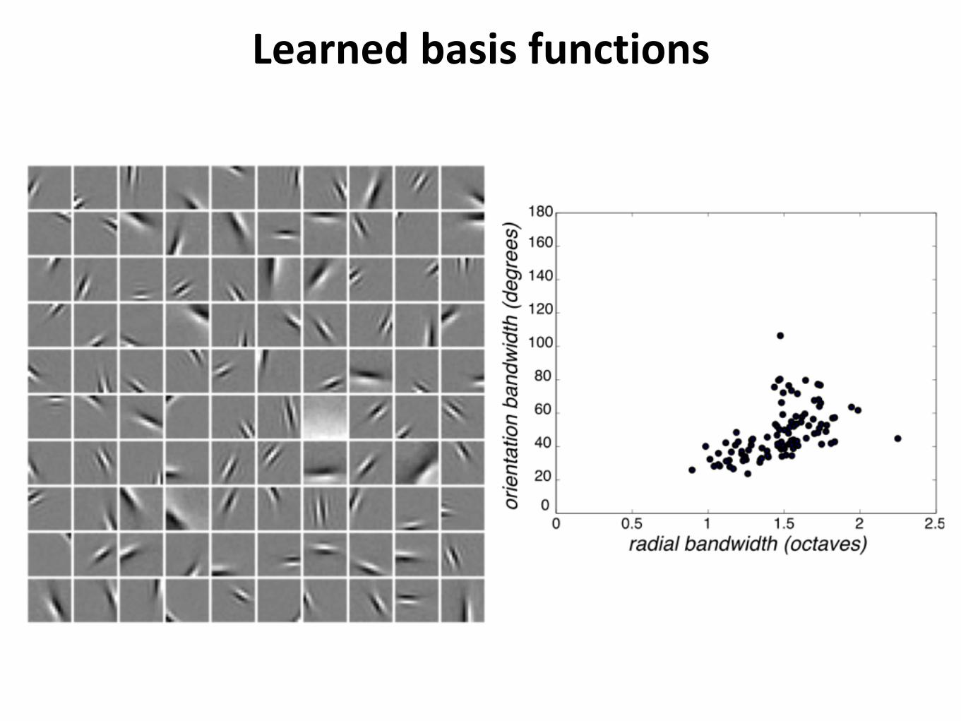
Learned  basis  functions

Applications of sparse coding

• Denoising / Inpainting / Super-resolution !

• Compressed sensing !

• Computer vision !

• Deep learning

Building high-level features using large-scale unsupervised learning

the cortex. They also demonstrate that convolutionalDBNs (Lee et al., 2009), trained on aligned images offaces, can learn a face detector. This result is inter-esting, but unfortunately requires a certain degree ofsupervision during dataset construction: their trainingimages (i.e., Caltech 101 images) are aligned, homoge-neous and belong to one selected category.

Figure 1. The architecture and parameters in one layer ofour network. The overall network replicates this structurethree times. For simplicity, the images are in 1D.

3.2. Architecture

Our algorithm is built upon these ideas and can beviewed as a sparse deep autoencoder with three impor-tant ingredients: local receptive fields, pooling and lo-cal contrast normalization. First, to scale the autoen-coder to large images, we use a simple idea known aslocal receptive fields (LeCun et al., 1998; Raina et al.,2009; Lee et al., 2009; Le et al., 2010). This biologi-cally inspired idea proposes that each feature in theautoencoder can connect only to a small region of thelower layer. Next, to achieve invariance to local defor-mations, we employ local L2 pooling (Hyvarinen et al.,2009; Gregor & LeCun, 2010; Le et al., 2010) and lo-cal contrast normalization (Jarrett et al., 2009). L2pooling, in particular, allows the learning of invariantfeatures (Hyvarinen et al., 2009; Le et al., 2010).

Our deep autoencoder is constructed by replicatingthree times the same stage composed of local filtering,local pooling and local contrast normalization. Theoutput of one stage is the input to the next one andthe overall model can be interpreted as a nine-layerednetwork (see Figure 1).

The first and second sublayers are often known as fil-tering (or simple) and pooling (or complex) respec-tively. The third sublayer performs local subtractiveand divisive normalization and it is inspired by bio-

logical and computational models (Pinto et al., 2008;Lyu & Simoncelli, 2008; Jarrett et al., 2009).2

As mentioned above, central to our approach is the useof local connectivity between neurons. In our experi-ments, the first sublayer has receptive fields of 18x18pixels and the second sub-layer pools over 5x5 over-lapping neighborhoods of features (i.e., pooling size).The neurons in the first sublayer connect to pixels in allinput channels (or maps) whereas the neurons in thesecond sublayer connect to pixels of only one channel(or map).3 While the first sublayer outputs linear filterresponses, the pooling layer outputs the square root ofthe sum of the squares of its inputs, and therefore, itis known as L2 pooling.

Our style of stacking a series of uniform mod-ules, switching between selectivity and toler-ance layers, is reminiscent of Neocognition andHMAX (Fukushima & Miyake, 1982; LeCun et al.,1998; Riesenhuber & Poggio, 1999). It has alsobeen argued to be an architecture employed by thebrain (DiCarlo et al., 2012).

Although we use local receptive fields, they arenot convolutional: the parameters are not sharedacross different locations in the image. This isa stark difference between our approach and pre-vious work (LeCun et al., 1998; Jarrett et al., 2009;Lee et al., 2009). In addition to being more biolog-ically plausible, unshared weights allow the learningof more invariances other than translational invari-ances (Le et al., 2010).

In terms of scale, our network is perhaps one of thelargest known networks to date. It has 1 billion train-able parameters, which is more than an order of magni-tude larger than other large networks reported in liter-ature, e.g., (Ciresan et al., 2010; Sermanet & LeCun,2011) with around 10 million parameters. It isworth noting that our network is still tiny com-pared to the human visual cortex, which is 106

times larger in terms of the number of neurons andsynapses (Pakkenberg et al., 2003).

3.3. Learning and Optimization

Learning: During learning, the parameters of thesecond sublayers (H) are fixed to uniform weights,

2The subtractive normalization removes theweighted average of neighboring neurons from thecurrent neuron gi,j,k = hi,j,k −

!

iuv Guvhi,j+u,i+v

The divisive normalization computes yi,j,k =gi,j,k/max{c, (

!

iuv Guvg2i,j+u,i+v)

0.5}, where c is setto be a small number, 0.01, to prevent numerical errors.G is a Gaussian weighting window. (Jarrett et al., 2009)

3For more details regarding connectivity patterns andparameter sensitivity, see Appendix B and E.

Deep learning!(Le et al. 2012 - aka ‘Google brain’

sparse coding

pooling

normalization

Building high-level features using large-scale unsupervised learning

the cortex. They also demonstrate that convolutionalDBNs (Lee et al., 2009), trained on aligned images offaces, can learn a face detector. This result is inter-esting, but unfortunately requires a certain degree ofsupervision during dataset construction: their trainingimages (i.e., Caltech 101 images) are aligned, homoge-neous and belong to one selected category.

Figure 1. The architecture and parameters in one layer ofour network. The overall network replicates this structurethree times. For simplicity, the images are in 1D.

3.2. Architecture

Our algorithm is built upon these ideas and can beviewed as a sparse deep autoencoder with three impor-tant ingredients: local receptive fields, pooling and lo-cal contrast normalization. First, to scale the autoen-coder to large images, we use a simple idea known aslocal receptive fields (LeCun et al., 1998; Raina et al.,2009; Lee et al., 2009; Le et al., 2010). This biologi-cally inspired idea proposes that each feature in theautoencoder can connect only to a small region of thelower layer. Next, to achieve invariance to local defor-mations, we employ local L2 pooling (Hyvarinen et al.,2009; Gregor & LeCun, 2010; Le et al., 2010) and lo-cal contrast normalization (Jarrett et al., 2009). L2pooling, in particular, allows the learning of invariantfeatures (Hyvarinen et al., 2009; Le et al., 2010).

Our deep autoencoder is constructed by replicatingthree times the same stage composed of local filtering,local pooling and local contrast normalization. Theoutput of one stage is the input to the next one andthe overall model can be interpreted as a nine-layerednetwork (see Figure 1).

The first and second sublayers are often known as fil-tering (or simple) and pooling (or complex) respec-tively. The third sublayer performs local subtractiveand divisive normalization and it is inspired by bio-

logical and computational models (Pinto et al., 2008;Lyu & Simoncelli, 2008; Jarrett et al., 2009).2

As mentioned above, central to our approach is the useof local connectivity between neurons. In our experi-ments, the first sublayer has receptive fields of 18x18pixels and the second sub-layer pools over 5x5 over-lapping neighborhoods of features (i.e., pooling size).The neurons in the first sublayer connect to pixels in allinput channels (or maps) whereas the neurons in thesecond sublayer connect to pixels of only one channel(or map).3 While the first sublayer outputs linear filterresponses, the pooling layer outputs the square root ofthe sum of the squares of its inputs, and therefore, itis known as L2 pooling.

Our style of stacking a series of uniform mod-ules, switching between selectivity and toler-ance layers, is reminiscent of Neocognition andHMAX (Fukushima & Miyake, 1982; LeCun et al.,1998; Riesenhuber & Poggio, 1999). It has alsobeen argued to be an architecture employed by thebrain (DiCarlo et al., 2012).

Although we use local receptive fields, they arenot convolutional: the parameters are not sharedacross different locations in the image. This isa stark difference between our approach and pre-vious work (LeCun et al., 1998; Jarrett et al., 2009;Lee et al., 2009). In addition to being more biolog-ically plausible, unshared weights allow the learningof more invariances other than translational invari-ances (Le et al., 2010).

In terms of scale, our network is perhaps one of thelargest known networks to date. It has 1 billion train-able parameters, which is more than an order of magni-tude larger than other large networks reported in liter-ature, e.g., (Ciresan et al., 2010; Sermanet & LeCun,2011) with around 10 million parameters. It isworth noting that our network is still tiny com-pared to the human visual cortex, which is 106

times larger in terms of the number of neurons andsynapses (Pakkenberg et al., 2003).

3.3. Learning and Optimization

Learning: During learning, the parameters of thesecond sublayers (H) are fixed to uniform weights,

2The subtractive normalization removes theweighted average of neighboring neurons from thecurrent neuron gi,j,k = hi,j,k −

!

iuv Guvhi,j+u,i+v

The divisive normalization computes yi,j,k =gi,j,k/max{c, (

!

iuv Guvg2i,j+u,i+v)

0.5}, where c is setto be a small number, 0.01, to prevent numerical errors.G is a Gaussian weighting window. (Jarrett et al., 2009)

3For more details regarding connectivity patterns andparameter sensitivity, see Appendix B and E.

Deep learning!(Le et al. 2012 - aka ‘Google brain’)

What is the dollar of Mexico?

Hyperdimensional computing

• High-dimensional representation (e.g., D = 10,000)

• Variables and values are combined into a “holistic” record using vector algebra:

“Multiplication” for binding

“Addition" for bundling

• Composed vector can in turn become a component in further composition

• Holistic record is decoded with (inverse) multiplication

• Approximate results of vector operations are identified with exact ones using content-addressable memory

See: Kanerva, P (2009) Hyperdimensional computing: An introduction to computing in distributed representations with high-dimensional random vectors. Cognitive Computation, 1(2): 139-159.

X = 1 0 0 1 0 ... 0 1!A = 0 0 1 1 1 ... 1 1

X*H = 0 1 1 1 0 ... 1 1 = A’ A⇠=

Y = 1 0 0 0 1 ... 1 0!B = 1 1 1 1 1 ... 0 0

Y*B = 0 1 1 1 0 ... 1 0 0 1 1 1 0 ... 1 0 ‘(y = b)’

Z = 0 1 1 0 1 ... 0 1!C = 1 0 0 0 1 ... 0 1

Z*C = 1 1 1 0 0 ... 0 0 1 1 1 0 0 ... 0 0 ‘(z = c)’

2 2 3 1 1 ... 2 0H = 1 1 1 0 0 ... 1 0

sumsum > 3/2

X = 1 0 0 1 0 ... 0 1 ‘unbind’

X*A = 1 0 1 0 1 ... 1 0 1 0 1 0 1 ... 1 0 ‘(x = a)’bind with XOR (*)

Item/clean-up memory finds nearest neighbor among known vectors

0 0 1 1 1 ... 1 1 = A

Example: H = X*A + Y*B + Z*C

lens eye is indeed specialized for looking up through the watersurface to exploit terrestrial or celestial visual cues.

With this result, it is tempting to speculate that the upperlens eye is used to detect the mangrove canopy throughSnell’s window, such that the approximately 1 cm largeanimals can find their habitat between the mangrove proproots and remain there even in the presence of tidal or storm-water currents. To evaluate the possibility that the upper lenseye detects the position of the mangrove canopy throughSnell’s window, we made still pictures using a wide-anglelens looking up through Snell’s window in the natural habitat.The pictures were taken from just under the surface to makeSnell’s window cover the same area of the surface as seenby the medusae. In the pictures, it was easy to follow themangrove canopy, which shifted from covering most of Snell’swindow to covering just the edge of Snell’s window when thecamera was slowly moved outward to about 20 m away fromthe lagoon edge (Figure 2).

To determine what medusae of T. cystophora would seewith their upper lens eyes, we used the optical model [2] ofthe eye to calculate the point-spread function of the optics atdifferent retinal locations. Applying these point-spread func-tions to still images of Snell’s window in themangrove swamp,we were able to simulate the retinal image formed in the upperlens eyes as a jellyfish moves about in the mangrove lagoon.The results (Figure 2) confirm that despite the severely under-focused eyes and blurred image [2], the approximately 5 m tallmangrove canopy can be readily detected at a distance of 4 mfrom the lagoon edge and, with some difficulty, can be de-tected even at a distance of 8 m (detection depends on theamount of surface ripple and the height of themangrove trees).These results thus predict that if T. cystophora medusae usetheir upper lens eyes to guide them to the correct habitat atthe lagoon edge, then they would swim toward this edge ifthey are closer than about 8 m away from it. Also, if they arefarther out in the lagoon, surface ripple and their poor visual

resolution will prevent detection of the mangrove canopy,and the animals would not be able to determine the directionto the closest lagoon edge.

Behavioral Assessment of Visual NavigationExperiments were conducted on wild populations ofT. cystophora medusae in the mangrove lagoons near LaParguera, Puerto Rico. Preliminary tests demonstrated that ifjellyfish were displaced about 5 m from their habitat at thelagoon edge, they rapidly swam back to the nearest edge,independent of compass orientation. To make controlledexperiments, we introduced a clear experimental tank consist-ing of a cylindrical wall and a flat bottom, open upward, to thenatural habitat under the mangrove canopy. When the tankwas filled with water, it was lightly buoyant such that the wallsextended 1–2 cm above the external water surface, effectivelysealing off the water around the animals but without affectingthe visual surroundings. A group of medusae was releasedin the tank, and as long as the tank remained under the canopy,the medusae showed no directional preference but occasion-ally bumped into the tank wall. The tank, with the trappedwater andmedusae, was then slowly towed out into the lagoonfrom the original position under themangrove canopy. In stepsof 2–4 m, starting at the canopy edge, the positions of themedusae within the tank were recorded by a video camerasuspended under the tank. At all positions, from the canopyedge and outward, the medusae ceased feeding and swamalong the edges of the tank, constantly bumping into it, sug-gesting that they responded to the displacement (Figure 3).Most importantly, their mean swimming direction differedsignificantly from random and coincided with the directiontoward the nearest mangrove trees (Table S1). This behaviorwas indicated already at the canopy edge but was strongestwhen the tank was placed 2 or 4 m into the lagoon (Figure 3).At 8 m from the canopy edge, the medusae could still detect

Figure 1. Rhopalial Orientation and Visual Fieldof the Upper Lens Eye

(A andB) In freely swimmingmedusae, the rhopa-lia maintain a constant vertical orientation. Whenthe medusa changes its body orientation, theheavy crystal (statolith) in the distal end of therhopalium causes the rhopalial stalk to bendsuch that the rhopalium remains verticallyoriented. Thus, the upper lens eye (ULE) pointsstraight upward at all times, irrespective ofbody orientation. The rhopalia in focus are situ-ated on the far side of the medusa and have theeyes directed to the center of the animal.(C) Modeling the receptive fields of the mostperipheral photoreceptors in the ULE (the relativeangular sensitivity of all peripheral rim photore-ceptors are superimposed and normalized ac-cording to the color template). The demarcatedfield of view reveals a near-perfect match to thesize and orientation of Snell’s window (dashedline).(D) The visual field of the ULE, of just below 100!,implies that it monitors the full 180! terrestrialscene, refracted through Snell’s window. LLEdenotes lower lens eye. Scale bars represent5 mm in (A) and (B) and 500 mm in insets.

Visual Navigation in Box Jellyfish799

jumping spider sand wasp

box jellyfish

Even ‘simple’ nervous systems can exhibit profound visual intelligence