What's Happened to the Phillips Curve? - Federal …s Happened to the Phillips Curve? Flint Brayton, John M. Roberts, and John C. Williams Division of Research and Statistics Federal

What's Happened to the Phillips Curve?

Flint Brayton, John M. Roberts, and John C. Williams�

Division of Research and StatisticsFederal Reserve Board

Washington, D.C. 20551

September 1999

Abstract

The simultaneous occurrence in the second half of the 1990s of low and falling priceinflation and low unemployment appears to be at odds with the properties of a standardPhillips curve. We find this result in a model in which inflation depends on the unem-ployment rate, past inflation, and conventional measures of price supply shocks. Weshow that, in such a model, long lags of past inflation are preferred to short lags, andthat with long lags, the NAIRU is estimated precisely but is unstable in the 1990s. Twoalternative modifications to the standard Phillips curve restore stability. One replacesthe unemployment rate with capacity utilization. Although this change leads to moreaccurate inflation predictions in the recent period, the predictive ability of the utiliza-tion rate is not superior to that of the unemployment rate for the 1955 to 1998 sampleas a whole. The second, and preferred, modification augments the standard Phillipscurve to include an “error-correction” mechanism involving the markup of prices overtrend unit labor costs. With the markup relatively high through much of the 1990s, thischannel is estimated to have held down inflation over this period, and thus provides anexplanation of the recent low inflation.

Keywords: Inflation, NAIRU, Phillips curve.

�The authors acknowledge the comments and assistance of Peter Tulip and the comments of Robert Gor-don and other participants at the 1999 NBER Summer Institute on Monetary Economics. Views presentedare those of the authors and do not necessarily represent those of the Federal Reserve Board or its staff.

1 Introduction and Summary

The rise and fall of inflation in the United States during the 1970s and 1980s provided a

testing ground for the Phillips curve model of inflation dynamics. And, according to some

observers (Fuhrer 1995, Gordon 1997), such models performed admirably well in tracking

actual inflation, both within and out of sample. Based on this achievement, many became

convinced of the usefulness of such models as tools in predicting inflation. Unfortunately,

the main feature of empirical Phillips curve models, that is, that inflation rises when labor

markets tighten, appears to be turned on its head during the economic expansion of the

1990s, when the unemployment rate fell below its long-run average of around 6 percent

and then slid under 5 percent, while inflation fell.

One objective of this paper is to ascertain whether the recent performance of infla-

tion is surprising in a statistical sense within the context of a canonical Phillips curve in

which price inflation depends on the unemployment rate, past price inflation, and standard

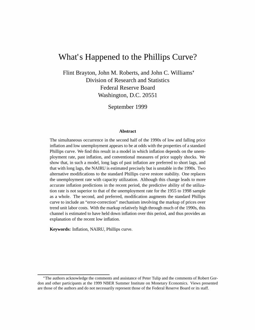
measures of price supply shocks. To provide a graphical preview of our conclusion that

a significant shift likely has taken place in such a baseline model, figure 1 shows forecast

errors for our preferred CPI equation.1 The upper panel of the figure contains one-quarter-

ahead forecast errors based on successive reestimates of the equation over samples whose

starting point is held fixed at 1955:Q1 and whose ending point advances one quarter at

a time. The forecasts make use of the actual values of explanatory variables.2 While no

individual error this decade lies outside of the 95 percent confidence range, inflation has

consistently fallen short of the model's predictions over the past five years.

Given the run of negative prediction errors, multi-period forecast errors and their con-

fidence bands provide a better graphical depiction of the probability of the equation's re-

cent performance. The lower panel of the figure plots the sequence of four-quarter-ahead

forecast errors. These errors are derived in a manner analogous to that used for the one-

1The inflation series is the the all-items CPI index, modified from 1967 to 1983 so that homeownershipcosts are on a rental-equivalent basis, and adjusted since 1995 to eliminate effects of methodological changes.The explanatory variables consist of twenty-four quarterly lags of past inflation; contemporaneous values ofa demographically weighted unemployment rate and a composite measure of relative food and energy pricemovements; an intercept; and a variable for the 1970s wage-price controls. The structure of this equation isdiscussed in more detail below.

2The use of forecasts conditional on actual values of explanatory variables is appropriate because the is-sues being examined concern the structure of the Phillips curve itself. Errors in forecasting the unemploymentrate, for example, are not germane because conceptually they are associated with the performance of otherequations in a forecasting system.

1

Figure

1CPI Inflation: Forecast Errors

(observations dated by end of forecast interval)(actual less predicted, annual rate)

-2

-1

0

1

2

95% confidence rangeone-quarter-ahead forecast error

1978 1980 1982 1984 1986 1988 1990 1992 1994 1996 1998-1.5

-1.0

-0.5

0.0

0.5

1.0

1.5four-quarter-ahead forecast error

2

step-ahead errors, except that within each four-quarter forecast interval, the forecast is a

dynamic simulation in which inflation lags are set equal to simulated values. The most

recent four-quarter forecasts have overpredicted inflation by as much as 1.3 percentage

points, well outside of the 95 percent confidence range, which encompasses forecast errors

of up to 0.9 percentage points.

A tendency to overpredict inflation starting in the middle of this decade characterizes

baseline equations for all six measures of inflation we study. For all but one, the magnitude

of the prediction errors is sufficient to reject the hypothesis of stability of the equation's

intercept at a significance level of 10 percent or lower. In the framework of these equa-

tions, instability of the intercept can be interpreted as instability of the NAIRU—that is, the

rate of unemployment consistent with stable inflation (Non-Accelerating Inflation Rate of

Unemployment).

We also find a close association between the number of lags of inflation included in the

baseline equations and whether or not evidence of significant structural change is found.

Equations such as ours with long inflation lags (up to twenty-four quarters) are generally

unstable while those with short lags are not. In essence, estimates of the NAIRU are much

more precise in long-lag equations than in short-lag equations, and consequently the level

of the unemployment rate over the past few years is well below the 95 percent NAIRU

confidence range of long-lag equations but not that of short-lag equations.

The relationship between inflation lag length and NAIRU precision has been docu-

mented by Staiger, Stock, and Watson (1997a)—hereafter, SSW—but they emphasize the

wide confidence intervals for the NAIRU found in short-lag equations on grounds that such

lag lengths are optimal according to either standard hypothesis tests or the use of infor-

mation criteria to select lag lengths. Our long-lag equations are the outcome of using an

information criteria to choose simultaneously lag lengths and coefficient smoothing re-

strictions. Permitting smoothing restrictions leads to equations that have much longer lags

on past inflation than is the case when lag coefficients are unrestricted, but with only a

few independently estimated parameters because the lag coefficients are restricted to lie on

low-order polynomials. We show that these long-lag Phillips curves, in addition to yielding

much more precise estimates of the NAIRU, have better out-of-sample forecasting proper-

ties than do the short-lag ones. Monte Carlo evidence indicates that the procedure of jointly

searching over lag lengths and smoothing restrictions is reasonably accurate at finding the

3

“correct” model, whether or not it contains smoothed inflation coefficients.

Our baseline analysis provides support for the type of Phillips curve long favored by

Robert Gordon who for many years has reported a specification with twenty-four quarterly

lags of past inflation.3 The tendency of our baseline equations to significantly overpredict

inflation since the mid-1990s, however, is an indication of structural change—perhaps a

decline of the NAIRU—or of misspecification. Because the baseline equations contain the

relative rates of import price inflation and food and energy price inflation, the statistical

evidence also permits the conclusion that recent declines in the relative prices of these

supply variables are not sufficient to account fully for the low rate of inflation.

We investigate two possible explanations for the breakdown or near-breakdown of the

standard Phillips curve. One is the possibility that the capacity utilization rate—which has

been near its historical average during the past few years—is a better measure of macroe-

conomic slack than the unemployment rate, in which case the recent behavior of inflation

would not be that extraordinary. From a conceptual perspective, the unemployment rate

might be preferred because of its broader sectoral coverage. But as it turns out, movements

of the utilization and unemployment rates are sufficiently similar over the past forty or so

years that the goodness of fit of equations based on one is quite similar to the fit of equa-

tions based on the other. Nonetheless, we find that Phillips curve equations that include the

unemployment rate fit somewhat better over the postwar years than do those using capacity

utilization. The outcome is closer to a toss up in out-of-sample forecasts, however. All told,

the evidence does not provide strong support for the use of capacity utilization but neither

does it suggest that the utilization rate is dominated by the unemployment rate.

Our preferred explanation is based on an augmented Phillips curve that includes the

level of the markup of price relative to trend unit labor costs as an error correction term.

We find that the level of the markup in the nonfarm business sector is highly significant in

equations for all measures of inflation examined, with a high markup estimated to restrain

inflation and a low markup putting upward pressure on inflation. Equations that include

the markup display much weaker evidence of instability. In particular, a high level of the

markup in the mid-1990s is estimated to have depressed price inflation through the late

1990s.3The most recent exposition is Gordon (1998).

4

2 Baseline equations

We examine the performance of standard Phillips curves for six measures of inflation,

CPI Consumer price index, all items,

CPIX Consumer price index, excluding food and energy,

PCE Personal consumption expenditures chain-weight price

PCEX Personal consumption expenditures, excluding food and energy,

chain-weight price,

GDP GDP chain-weight price,

NFB Nonfarm business, excluding housing, chain-weight price,

over a sample period that extends most frequently from 1955:Q1 to 1998:Q4. Data avail-

ability limits the start of estimation periods for CPIX and PCEX equations to 1963:Q3 and

1965:Q3, respectively, after making allowance for the maximum number of inflation lags

we consider.

A similar strategy of estimation and testing is applied to each measure of inflation. First,

a list of potential explanatory variables is chosen, and then a data-based testing procedure

is used to select which variables and how many lags to include in each inflation equation.

Finally, to examine whether the inflation process has changed in some significant way, the

coefficients of each estimated equation are tested for constancy using a procedure that does

not require a prior belief about the precise date of the change.

2.1 Selecting explanatory variables and lag lengths

In the baseline specification, the list of potential explanatory variables consists of lags of

inflation, a demographically weighted unemployment rate, and two measures of supply

shocks: the rates of relative price inflation of imports and a food-energy aggregate.4 When

initially considering how to determine lag lengths for explanatory variables, we noted that

Gordon for many years has reported equations with twenty-four inflation lags while SSW

(1997a) focus their attention on equations with only a year's worth of quarterly or monthly

lags. These two specifications represent very different approaches to economizing on the

number of freely estimated parameters on lagged inflation. Gordon achieves parsimony

4All equations also include a constant and a dummy variable for wage and price controls in the 1970s.

5

through the use of successive four-quarter averages of lags of inflation. Thus, his twenty-

four lags require the estimation of only six coefficients (on lags 1-4, 5-8, etc.). SSW, on

the other hand, estimate models in which each lag of inflation has a independent coefficient

and frequently use an information criterion to choose the “best” number of lags.

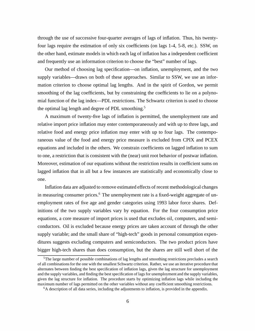
Our method of choosing lag specification—on inflation, unemployment, and the two

supply variables—draws on both of these approaches. Similar to SSW, we use an infor-

mation criterion to choose optimal lag lengths. And in the spirit of Gordon, we permit

smoothing of the lag coefficients, but by constraining the coefficients to lie on a polyno-

mial function of the lag index—PDL restrictions. The Schwartz criterion is used to choose

the optimal lag length and degree of PDL smoothing.5

A maximum of twenty-five lags of inflation is permitted, the unemployment rate and

relative import price inflation may enter contemporaneously and with up to three lags, and

relative food and energy price inflation may enter with up to four lags. The contempo-

raneous value of the food and energy price measure is excluded from CPIX and PCEX

equations and included in the others. We constrain coefficients on lagged inflation to sum

to one, a restriction that is consistent with the (near) unit root behavior of postwar inflation.

Moreover, estimation of our equations without the restriction results in coefficient sums on

lagged inflation that in all but a few instances are statistically and economically close to

one.

Inflation data are adjusted to remove estimated effects of recent methodological changes

in measuring consumer prices.6 The unemployment rate is a fixed-weight aggregate of un-

employment rates of five age and gender categories using 1993 labor force shares. Def-

initions of the two supply variables vary by equation. For the four consumption price

equations, a core measure of import prices is used that excludes oil, computers, and semi-

conductors. Oil is excluded because energy prices are taken account of through the other

supply variable; and the small share of “high-tech” goods in personal consumption expen-

ditures suggests excluding computers and semiconductors. The two product prices have

bigger high-tech shares than does consumption, but the shares are still well short of the

5The large number of possible combinations of lag lengths and smoothing restrictions precludes a searchof all combinations for the one with the smallest Schwartz criterion. Rather, we use an iterative procedure thatalternates between finding the best specification of inflation lags, given the lag structure for unemploymentand the supply variables, and finding the best specification of lags for unemployment and the supply variables,given the lag structure for inflation. The procedure starts by optimizing inflation lags while including themaximum number of lags permitted on the other variables without any coefficient smoothing restrictions.

6A description of all data series, including the adjustments to inflation, is provided in the appendix.

6

contribution of such goods to imports. Roughly speaking, GDP has about one-tenth the

computer and semiconductor share of imports. Consequently, the import price series we

use in the product price equations includes one-tenth the contribution of computers and

semiconductors to import prices. Relative import price inflation is constructed by subtract-

ing from the appropriate measure of import price inflation the once-lagged value of the

aggregate inflation series being explained. The second supply variable, relative food and

energy price inflation, is measured as the difference between overall and core CPI inflation

in the two CPI equations and as the difference between overall and core PCE inflation in

the others.7

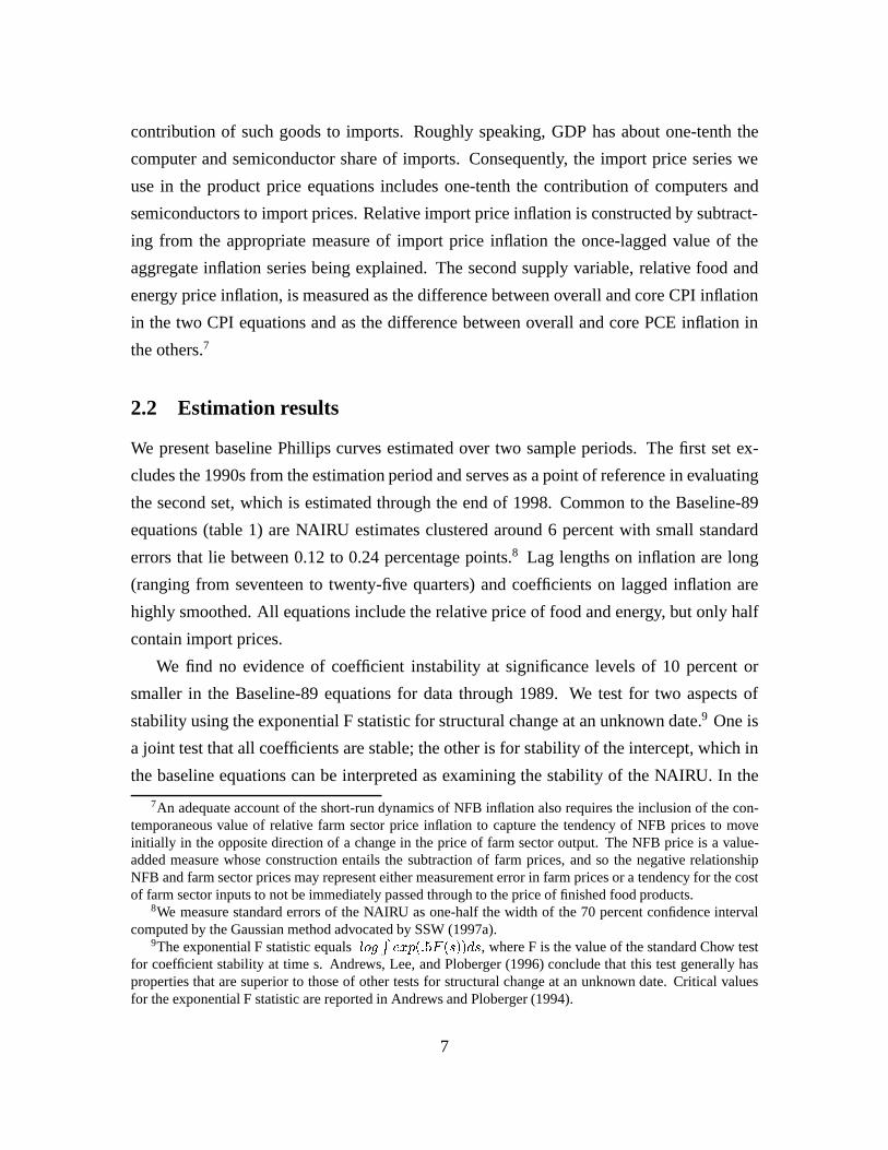
2.2 Estimation results

We present baseline Phillips curves estimated over two sample periods. The first set ex-

cludes the 1990s from the estimation period and serves as a point of reference in evaluating

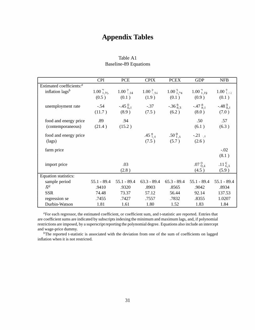
the second set, which is estimated through the end of 1998. Common to the Baseline-89

equations (table 1) are NAIRU estimates clustered around 6 percent with small standard

errors that lie between 0.12 to 0.24 percentage points.8 Lag lengths on inflation are long

(ranging from seventeen to twenty-five quarters) and coefficients on lagged inflation are

highly smoothed. All equations include the relative price of food and energy, but only half

contain import prices.

We find no evidence of coefficient instability at significance levels of 10 percent or

smaller in the Baseline-89 equations for data through 1989. We test for two aspects of

stability using the exponential F statistic for structural change at an unknown date.9 One is

a joint test that all coefficients are stable; the other is for stability of the intercept, which in

the baseline equations can be interpreted as examining the stability of the NAIRU. In the

7An adequate account of the short-run dynamics of NFB inflation also requires the inclusion of the con-temporaneous value of relative farm sector price inflation to capture the tendency of NFB prices to moveinitially in the opposite direction of a change in the price of farm sector output. The NFB price is a value-added measure whose construction entails the subtraction of farm prices, and so the negative relationshipNFB and farm sector prices may represent either measurement error in farm prices or a tendency for the costof farm sector inputs to not be immediately passed through to the price of finished food products.

8We measure standard errors of the NAIRU as one-half the width of the 70 percent confidence intervalcomputed by the Gaussian method advocated by SSW (1997a).

9The exponential F statistic equalslogRexp(:5F (s))ds, where F is the value of the standard Chow test

for coefficient stability at time s. Andrews, Lee, and Ploberger (1996) conclude that this test generally hasproperties that are superior to those of other tests for structural change at an unknown date. Critical valuesfor the exponential F statistic are reported in Andrews and Ploberger (1994).

7

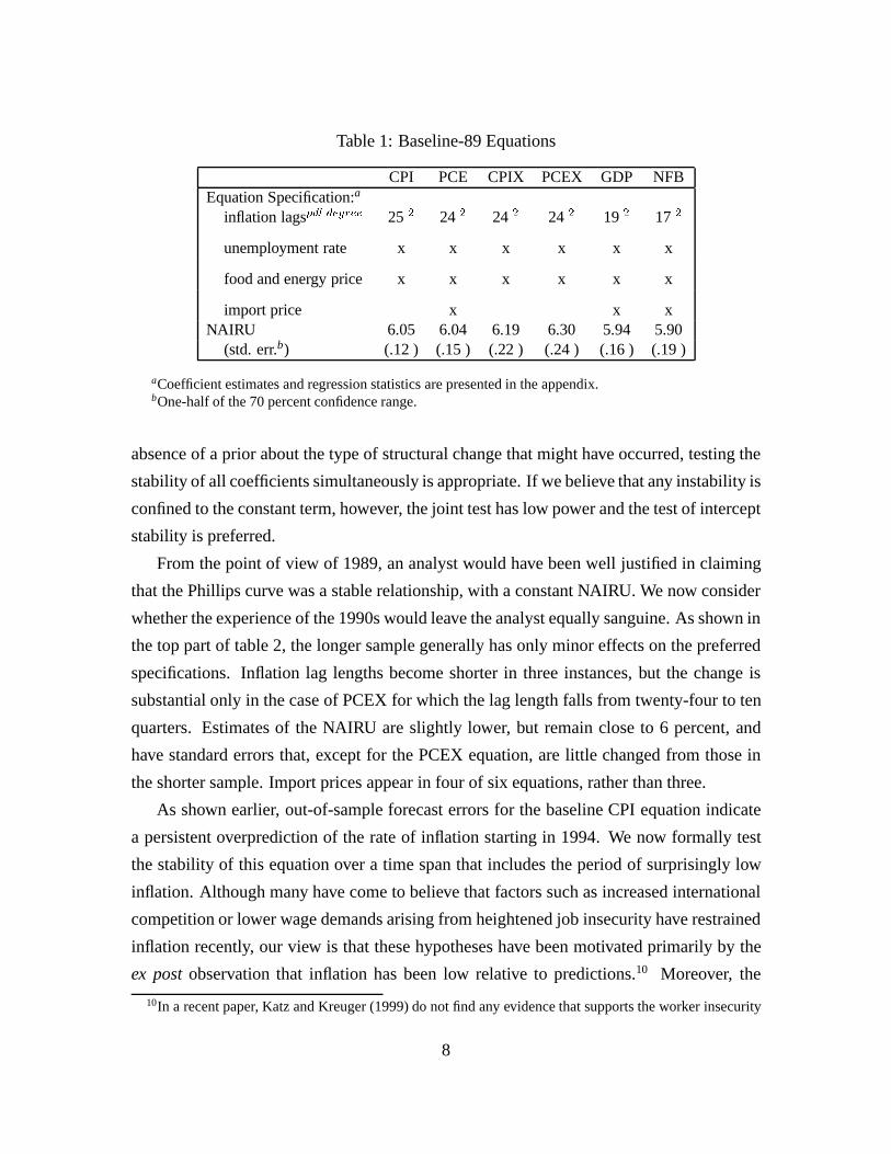
Table 1: Baseline-89 Equations

CPI PCE CPIX PCEX GDP NFBEquation Specification:a

inflation lagspdl degree 25 2 24 2 24 2 24 2 19 2 17 2

unemployment rate x x x x x x

food and energy price x x x x x x

import price x x xNAIRU 6.05 6.04 6.19 6.30 5.94 5.90

(std. err.b) (.12 ) (.15 ) (.22 ) (.24 ) (.16 ) (.19 )

aCoefficient estimates and regression statistics are presented in the appendix.bOne-half of the 70 percent confidence range.

absence of a prior about the type of structural change that might have occurred, testing the

stability of all coefficients simultaneously is appropriate. If we believe that any instability is

confined to the constant term, however, the joint test has low power and the test of intercept

stability is preferred.

From the point of view of 1989, an analyst would have been well justified in claiming

that the Phillips curve was a stable relationship, with a constant NAIRU. We now consider

whether the experience of the 1990s would leave the analyst equally sanguine. As shown in

the top part of table 2, the longer sample generally has only minor effects on the preferred

specifications. Inflation lag lengths become shorter in three instances, but the change is

substantial only in the case of PCEX for which the lag length falls from twenty-four to ten

quarters. Estimates of the NAIRU are slightly lower, but remain close to 6 percent, and

have standard errors that, except for the PCEX equation, are little changed from those in

the shorter sample. Import prices appear in four of six equations, rather than three.

As shown earlier, out-of-sample forecast errors for the baseline CPI equation indicate

a persistent overprediction of the rate of inflation starting in 1994. We now formally test

the stability of this equation over a time span that includes the period of surprisingly low

inflation. Although many have come to believe that factors such as increased international

competition or lower wage demands arising from heightened job insecurity have restrained

inflation recently, our view is that these hypotheses have been motivated primarily by the

ex postobservation that inflation has been low relative to predictions.10 Moreover, the

10In a recent paper, Katz and Kreuger (1999) do not find any evidence that supports the worker insecurity

8

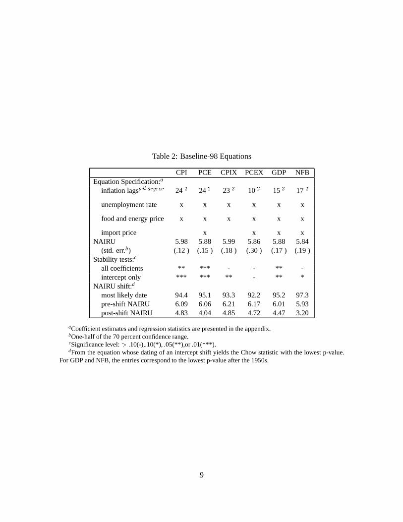
Table 2: Baseline-98 Equations





import price x x x xNAIRU 5.98 5.88 5.99 5.86 5.88 5.84

(std. err.b) (.12 ) (.15 ) (.18 ) (.30 ) (.17 ) (.19 )Stability tests:c

all coefficients ** *** - - ** -intercept only *** *** ** - ** *

NAIRU shift:d

most likely date 94.4 95.1 93.3 92.2 95.2 97.3pre-shift NAIRU 6.09 6.06 6.21 6.17 6.01 5.93post-shift NAIRU 4.83 4.04 4.85 4.72 4.47 3.20

aCoefficient estimates and regression statistics are presented in the appendix.bOne-half of the 70 percent confidence range.cSignificance level:> .10(-),.10(*), .05(**),or .01(***).dFrom the equation whose dating of an intercept shift yields the Chow statistic with the lowest p-value.

For GDP and NFB, the entries correspond to the lowest p-value after the 1950s.

9

conjectures do not provide any independent information about the likely date of a shift in

the inflation process. Thus, in the absence of a specific prior, we assess the stability of

the CPI equation at all dates in the full estimation period, which runs from 1955:Q1 to

1998:Q4.

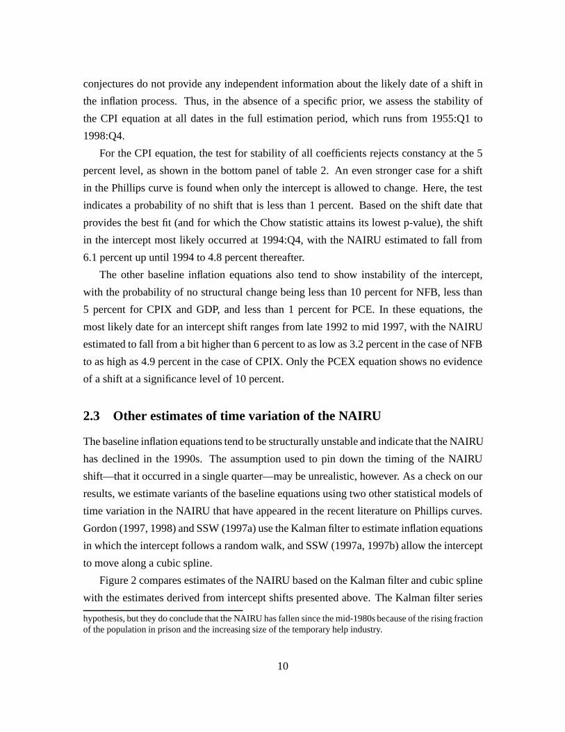
For the CPI equation, the test for stability of all coefficients rejects constancy at the 5

percent level, as shown in the bottom panel of table 2. An even stronger case for a shift

in the Phillips curve is found when only the intercept is allowed to change. Here, the test

indicates a probability of no shift that is less than 1 percent. Based on the shift date that

provides the best fit (and for which the Chow statistic attains its lowest p-value), the shift

in the intercept most likely occurred at 1994:Q4, with the NAIRU estimated to fall from

6.1 percent up until 1994 to 4.8 percent thereafter.

The other baseline inflation equations also tend to show instability of the intercept,

with the probability of no structural change being less than 10 percent for NFB, less than

5 percent for CPIX and GDP, and less than 1 percent for PCE. In these equations, the

most likely date for an intercept shift ranges from late 1992 to mid 1997, with the NAIRU

estimated to fall from a bit higher than 6 percent to as low as 3.2 percent in the case of NFB

to as high as 4.9 percent in the case of CPIX. Only the PCEX equation shows no evidence

of a shift at a significance level of 10 percent.

2.3 Other estimates of time variation of the NAIRU

The baseline inflation equations tend to be structurally unstable and indicate that the NAIRU

has declined in the 1990s. The assumption used to pin down the timing of the NAIRU

shift—that it occurred in a single quarter—may be unrealistic, however. As a check on our

results, we estimate variants of the baseline equations using two other statistical models of

time variation in the NAIRU that have appeared in the recent literature on Phillips curves.

Gordon (1997, 1998) and SSW (1997a) use the Kalman filter to estimate inflation equations

in which the intercept follows a random walk, and SSW (1997a, 1997b) allow the intercept

to move along a cubic spline.

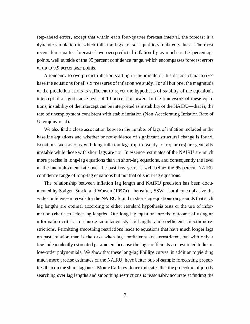
Figure 2 compares estimates of the NAIRU based on the Kalman filter and cubic spline

with the estimates derived from intercept shifts presented above. The Kalman filter series

hypothesis, but they do conclude that the NAIRU has fallen since the mid-1980s because of the rising fractionof the population in prison and the increasing size of the temporary help industry.

10

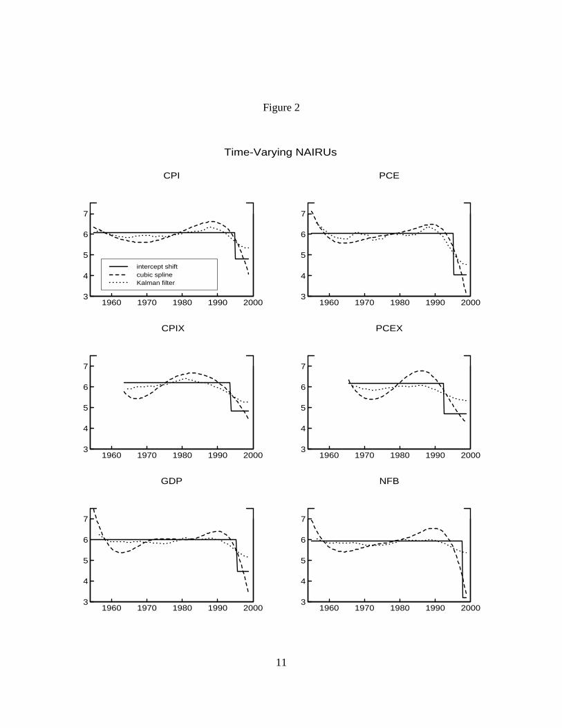
Figure 2

3

4

5

6

7

1960 1970 1980 1990 2000

CPI

intercept shiftcubic splineKalman filter

3

4

5

6

7

1960 1970 1980 1990 2000

PCE

3

4

5

6

7

1960 1970 1980 1990 2000

CPIX

3

4

5

6

7

1960 1970 1980 1990 2000

PCEX

3

4

5

6

7

1960 1970 1980 1990 2000

GDP

3

4

5

6

7

1960 1970 1980 1990 2000

NFB

Time-Varying NAIRUs

11

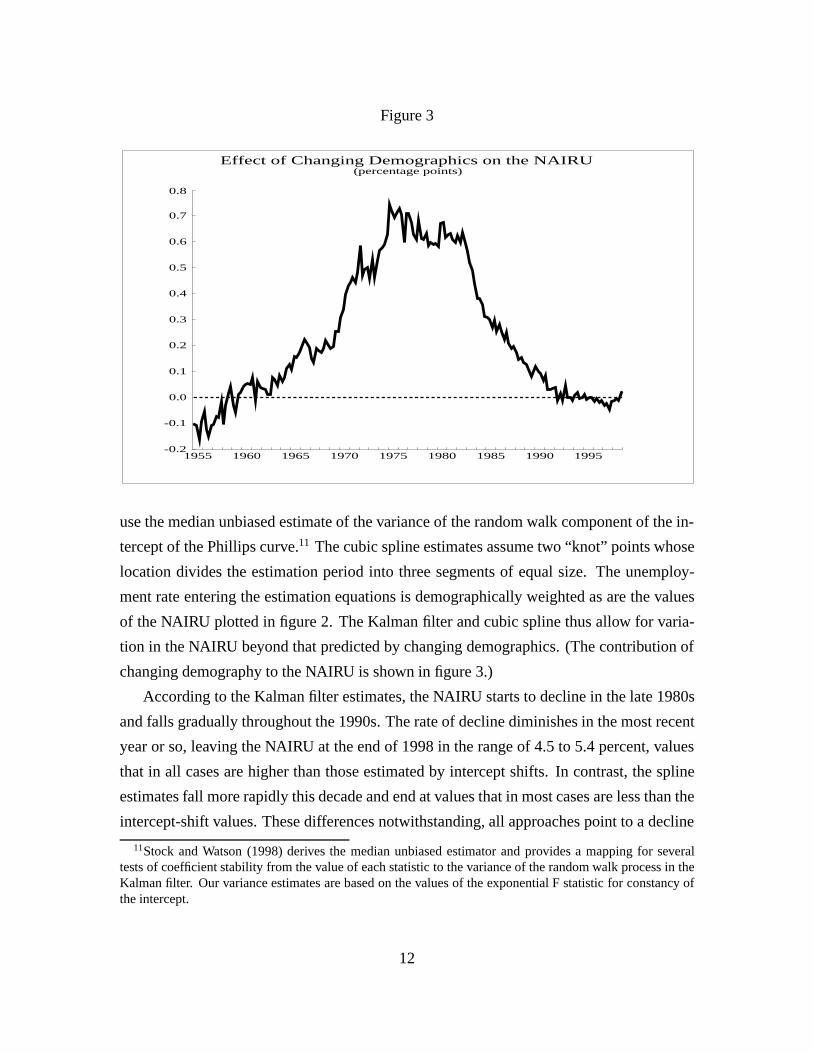
Figure 3

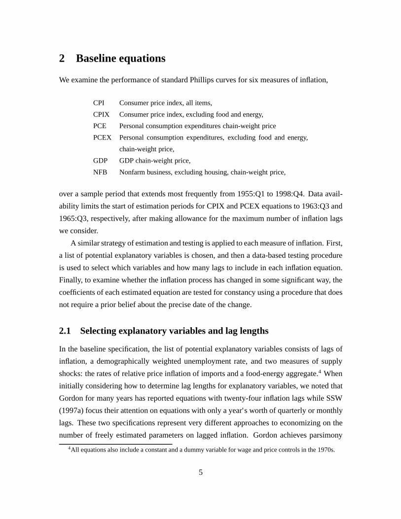
Effect of Changing Demographics on the NAIRU(percentage points)

1955 1960 1965 1970 1975 1980 1985 1990 1995-0.2

-0.1

0.0

0.1

0.2

0.3

0.4

0.5

0.6

0.7

0.8

use the median unbiased estimate of the variance of the random walk component of the in-

tercept of the Phillips curve.11 The cubic spline estimates assume two “knot” points whose

location divides the estimation period into three segments of equal size. The unemploy-

ment rate entering the estimation equations is demographically weighted as are the values

of the NAIRU plotted in figure 2. The Kalman filter and cubic spline thus allow for varia-

tion in the NAIRU beyond that predicted by changing demographics. (The contribution of

changing demography to the NAIRU is shown in figure 3.)

According to the Kalman filter estimates, the NAIRU starts to decline in the late 1980s

and falls gradually throughout the 1990s. The rate of decline diminishes in the most recent

year or so, leaving the NAIRU at the end of 1998 in the range of 4.5 to 5.4 percent, values

that in all cases are higher than those estimated by intercept shifts. In contrast, the spline

estimates fall more rapidly this decade and end at values that in most cases are less than the

intercept-shift values. These differences notwithstanding, all approaches point to a decline

11Stock and Watson (1998) derives the median unbiased estimator and provides a mapping for severaltests of coefficient stability from the value of each statistic to the variance of the random walk process in theKalman filter. Our variance estimates are based on the values of the exponential F statistic for constancy ofthe intercept.

12

in the NAIRU in the 1990s that in almost every case is larger in magnitude than movements

in the NAIRU at any earlier time in the period under consideration.

2.4 Import prices

A common belief is that low import prices have been a substantial restraint on domestic

inflation in the late 1990s. Over the four years from 1995 to 1998, the measures of import

price inflation we use have increased between 2 and 3 percentage points more slowly at an

annual rate, on average, than have the consumption and product prices under examination.

Given the estimated coefficients on the relative rate of increase of import prices (between

.04 and .12), these declines reduce the average (static) inflation prediction only about a

tenth of a percentage point in the PCE, PCEX, and GDP equations, and about two tenths of

a percentage point in the NFB equation. However, because these effects are small relative

to the mean residuals of these equations over the 1995-1998 period (from 0.4 to 0.7 per-

centage points), we conclude that import prices have made a modest, but not substantial,

contribution to holding down domestic inflation.12

An alternative analysis of the contribution of import prices focuses not only on the

declining relative price of imports but also on the possibility of an increase in the sensitivity

of domestic prices to the price of imports. And, indeed, statistical tests reveal that constancy

of import price coefficients is rejected at the 1 percent level for PCE, at the 5 percent

level for GDP, and at the 10 percent level for NFB. Two observations suggest the strong

probability that these results are spurious, however. One is that it is difficult to distinguish

in the mid-1990s a shift in the intercept from a shift in the import price coefficients, because

of a downward shift in the mean of the relative rate of import price inflation that occurred

around that time. Conditional on there being an intercept shift, evidence for a shift in import

price coefficients significantly weakens, and similarly, conditional on a shift in import price

coefficients, evidence for a shift in intercepts significantly weakens.

12As noted earlier, computers and semiconductors are wholly excluded in the import price measure usedin consumption price equations and largely excluded in the measure entering product price equations. Givenrapid declines in the prices of computers and semiconductors and their relatively large share in imports,import prices inclusive of these goods fall about 3 percentage points more rapidly at an annual rate, onaverage, over the 1995-1998 period than do measures that exclude them. If the model selection procedureis run with the broader measure of import prices in the set of explanatory variables, we find that, comparedwith the Baseline-98 results, import prices are included in the same four equations, but that in those equationsrecent errors are slightly smaller and the statistical significance of an intercept shift is modestly reduced.

13

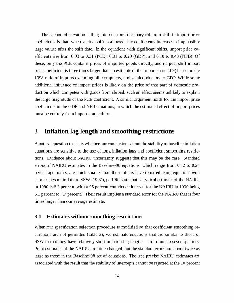
The second observation calling into question a primary role of a shift in import price

coefficients is that, when such a shift is allowed, the coefficients increase to implausibly

large values after the shift date. In the equations with significant shifts, import price co-

efficients rise from 0.03 to 0.31 (PCE), 0.01 to 0.20 (GDP), and 0.10 to 0.48 (NFB). Of

these, only the PCE contains prices of imported goods directly, and its post-shift import

price coefficient is three times larger than an estimate of the import share (.09) based on the

1998 ratio of imports excluding oil, computers, and semiconductors to GDP. While some

additional influence of import prices is likely on the price of that part of domestic pro-

duction which competes with goods from abroad, such an effect seems unlikely to explain

the large magnitude of the PCE coefficient. A similar argument holds for the import price

coefficients in the GDP and NFB equations, in which the estimated effect of import prices

must be entirely from import competition.

3 Inflation lag length and smoothing restrictions

A natural question to ask is whether our conclusions about the stability of baseline inflation

equations are sensitive to the use of long inflation lags and coefficient smoothing restric-

tions. Evidence about NAIRU uncertainty suggests that this may be the case. Standard

errors of NAIRU estimates in the Baseline-98 equations, which range from 0.12 to 0.24

percentage points, are much smaller than those others have reported using equations with

shorter lags on inflation. SSW (1997a, p. 196) state that “a typical estimate of the NAIRU

in 1990 is 6.2 percent, with a 95 percent confidence interval for the NAIRU in 1990 being

5.1 percent to 7.7 percent.” Their result implies a standard error for the NAIRU that is four

times larger than our average estimate.

3.1 Estimates without smoothing restrictions

When our specification selection procedure is modified so that coefficient smoothing re-

strictions are not permitted (table 3), we estimate equations that are similar to those of

SSW in that they have relatively short inflation lag lengths—from four to seven quarters.

Point estimates of the NAIRU are little changed, but the standard errors are about twice as

large as those in the Baseline-98 set of equations. The less precise NAIRU estimates are

associated with the result that the stability of intercepts cannot be rejected at the 10 percent

14

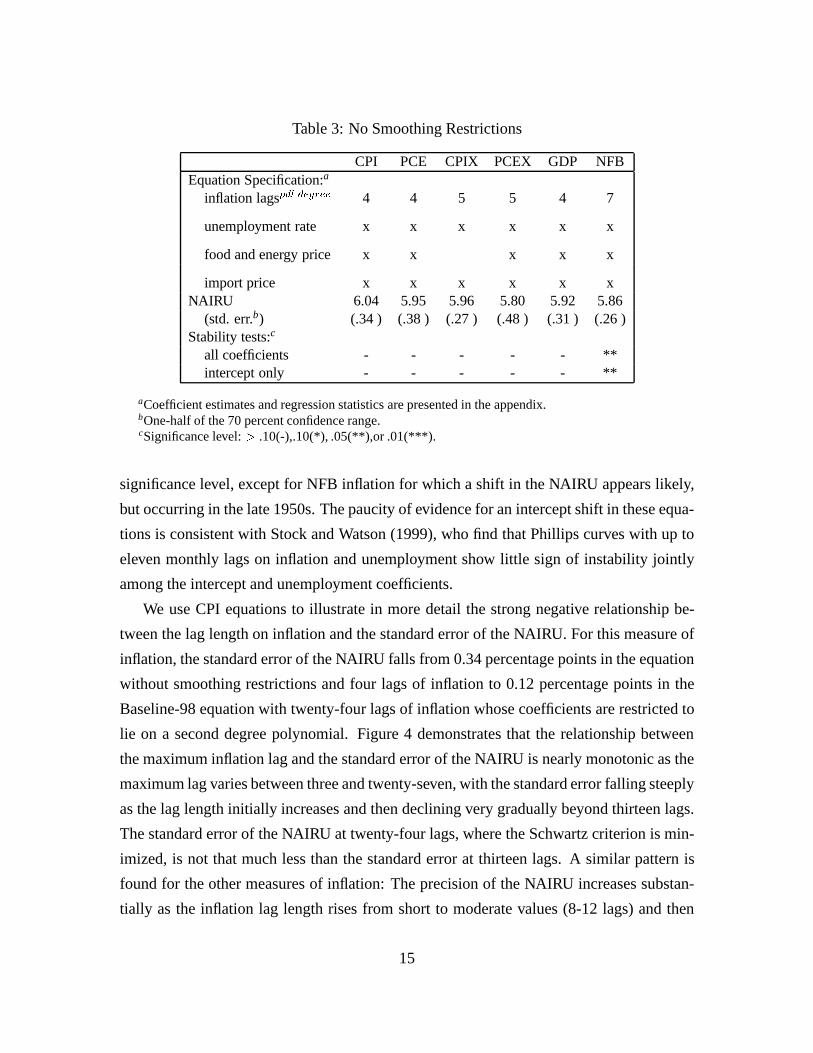
Table 3: No Smoothing Restrictions


inflation lagspdl degree 4 4 5 5 4 7


food and energy price x x x x x

import price x x x x x xNAIRU 6.04 5.95 5.96 5.80 5.92 5.86


all coefficients - - - - - **intercept only - - - - - **

aCoefficient estimates and regression statistics are presented in the appendix.bOne-half of the 70 percent confidence range.cSignificance level:> .10(-),.10(*), .05(**),or .01(***).

significance level, except for NFB inflation for which a shift in the NAIRU appears likely,

but occurring in the late 1950s. The paucity of evidence for an intercept shift in these equa-

tions is consistent with Stock and Watson (1999), who find that Phillips curves with up to

eleven monthly lags on inflation and unemployment show little sign of instability jointly

among the intercept and unemployment coefficients.

We use CPI equations to illustrate in more detail the strong negative relationship be-

tween the lag length on inflation and the standard error of the NAIRU. For this measure of

inflation, the standard error of the NAIRU falls from 0.34 percentage points in the equation

without smoothing restrictions and four lags of inflation to 0.12 percentage points in the

Baseline-98 equation with twenty-four lags of inflation whose coefficients are restricted to

lie on a second degree polynomial. Figure 4 demonstrates that the relationship between

the maximum inflation lag and the standard error of the NAIRU is nearly monotonic as the

maximum lag varies between three and twenty-seven, with the standard error falling steeply

as the lag length initially increases and then declining very gradually beyond thirteen lags.

The standard error of the NAIRU at twenty-four lags, where the Schwartz criterion is min-

imized, is not that much less than the standard error at thirteen lags. A similar pattern is

found for the other measures of inflation: The precision of the NAIRU increases substan-

tially as the inflation lag length rises from short to moderate values (8-12 lags) and then

15

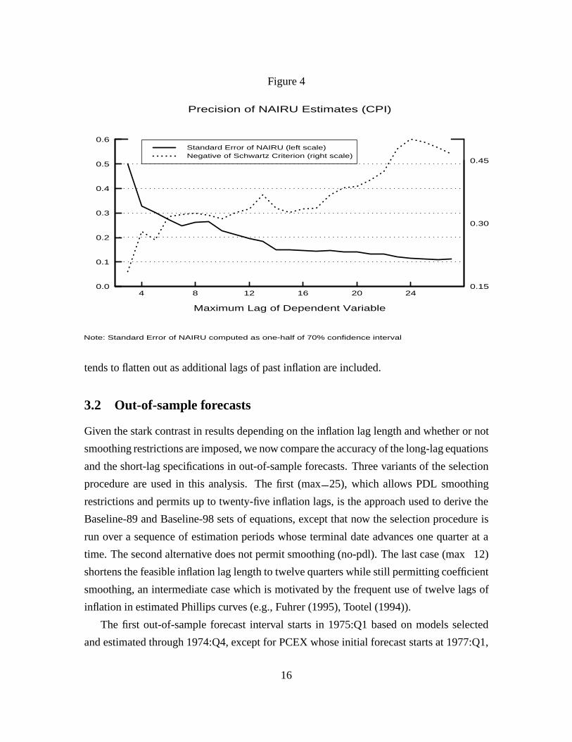
Figure 4

0.0

0.1

0.2

0.3

0.4

0.5

0.6

4 8 12 16 20 240.15

0.30

0.45

Standard Error of NAIRU (left scale)Negative of Schwartz Criterion (right scale)

Maximum Lag of Dependent Variable

Precision of NAIRU Estimates (CPI)

Note: Standard Error of NAIRU computed as one-half of 70% confidence interval

tends to flatten out as additional lags of past inflation are included.

3.2 Out-of-sample forecasts

Given the stark contrast in results depending on the inflation lag length and whether or not

smoothing restrictions are imposed, we now compare the accuracy of the long-lag equations

and the short-lag specifications in out-of-sample forecasts. Three variants of the selection

procedure are used in this analysis. The first (max=25), which allows PDL smoothing

restrictions and permits up to twenty-five inflation lags, is the approach used to derive the

Baseline-89 and Baseline-98 sets of equations, except that now the selection procedure is

run over a sequence of estimation periods whose terminal date advances one quarter at a

time. The second alternative does not permit smoothing (no-pdl). The last case (max=12)

shortens the feasible inflation lag length to twelve quarters while still permitting coefficient

smoothing, an intermediate case which is motivated by the frequent use of twelve lags of

inflation in estimated Phillips curves (e.g., Fuhrer (1995), Tootel (1994)).

The first out-of-sample forecast interval starts in 1975:Q1 based on models selected

and estimated through 1974:Q4, except for PCEX whose initial forecast starts at 1977:Q1,

16

Table 4: Out-of-Sample Forecast RMSEs

(percent)CPI PCE CPIX PCEX GDP NFB

Four-Quarters-Aheadmaxlag=25 .60 .72 1.25 .93 .73 1.02maxlag=12 .77 .74 .76 .76 .76 1.04no-pdl .85 .82 1.04 .76 .95 1.53

Eight-Quarters-Aheadmaxlag=25 1.23 1.45 2.63 2.04 1.42 1.86maxlag=12 1.82 1.51 1.60 1.48 1.33 1.79no-pdl 2.14 1.78 2.77 1.68 2.24 3.42

given the shorter historical time span over which data on this measure of inflation is avail-

able. For all inflation measures, the last forecast period ends at 1998:Q4. The results in

table 4, which reports root mean squared percentage forecast errors for the price level at

horizons of four and eight quarters, confirm the conclusion based on in-sample results that

long-lag inflation equations tend to be superior to short-lag ones. In nine of twelve cases,

our model selection procedure (max=25) yields price-level forecasts that have smaller root

mean squared errors than does the procedure not permitting coefficient smoothing (no-pdl).

In some cases, however, the intermediate procedure (max=12), in which smoothing restric-

tions are permissible but inflation lag lengths are constrained to be no more than twelve

quarters, yields more accurate forecasts than does the longer-lag variant.

3.3 Monte Carlo analysis

In this section, we report four experiments with models of CPI inflation designed to address

the question of whether model-selection criteria can discriminate between long-lag and

short-lag models of the Phillips curve in samples such as the one we are examining. In

the first two experiments, we repeatedly generate artificial data assuming that our long-lag,

low-order model for own-lags in the Phillips curve is the correct model (table 2, column

1) and then run two different model-selection procedures, one of which allows for the

possibility of polynomial smoothing restrictions, and the other of which does not. In the

next pair of experiments, we generate sets of artificial data assuming the true model is

such that inflation lags are short and unrestricted (table 3, column 1). We then run the two

different model-selection exercises on each set of artificial data.

17

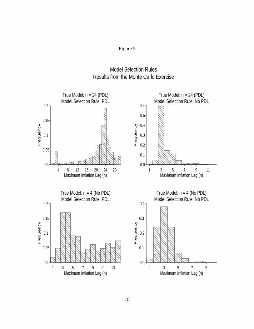
Figure 5

4 8 12 16 20 24 280.0

0.05

0.1

0.15

0.2

True Model: n = 24 (PDL)Model Selection Rule: PDL

Maximum Inflation Lag (n)

Fre

qu

en

cy

1 3 5 7 9 110.0

0.1

0.2

0.3

0.4

0.5

0.6


Model Selection RulesResults from the Monte Carlo Exercise

True Model: n = 24 (PDL)Model Selection Rule: No PDL

Fre

qu

en

cy

1 3 5 7 9 11 130.0

0.05

0.1

0.15

0.2


True Model: n = 4 (No PDL)Model Selection Rule: PDL

Fre

qu

en

cy

1 3 5 7 90.0

0.1

0.2

0.3

0.4


Fre

qu

en

cy

True Model: n = 4 (No PDL)Model Selection Rule: No PDL

18

We use a six-lag VAR to generate simulated data for the other endogenous variables in

the model, namely, the unemployment rate; the relative food-and-energy price; and relative

import prices. We assume that the unemployment rate is unaffected in the current period by

any of the other variables in the model; that relative food-and-energy prices are affected by

the unemployment rate but not by any of the other variables; and that relative import prices

are affected by unemployment and food-and-energy prices but not aggregate inflation.

Based on one thousand draws, we find that when the model used to generate the artificial

data is the long-lags version of the Phillips curve, the specification-search procedure that

allows for smoothing restrictions generally chooses long lags (figure 5, upper left panel),

and that the search procedure which does not allow for smoothing restrictions selects a

short-lag model (upper right panel). In particular, the median lag length when smoothing

restrictions are allowed is twenty-three, compared to the true lag length of twenty-four

(with the coefficients constrained to lie on a second-order polynomial). In 75 percent of the

draws, the chosen lag length is twenty or more. In only 5 percent of the draws is the chosen

lag length four or less. By contrast, when only unconstrained lags are allowed, the median

lag length chosen is three, and in 99 percent of cases the chosen lag length is ten or less.

When the true model involves low order and long lags, a model-specification procedure

that does not allow for this possibility will choose a specification with far too few lags.

As noted previously, when we run the model-specification search for a model for the

CPI allowing only for unconstrained own-lag specifications, the procedure chooses four

lags. Using this specification to generate artificial data, the median number of lags chosen

when the model search procedure is limited to consider only unconstrained lags is three

(lower right panel), and in 95 percent of the cases, the number of lags is five or fewer.

When reduced-order polynomials are allowed, the median number of lags selected is six

while the ninety-fifth percentile of the distribution is fourteen lags (lower left panel).

On the whole, the more-general model-selection procedure that allows low-order poly-

nomials out-performs the procedure that permits only unrestricted lags. The median lag

estimated by the first method is close to the inflation lag length used to generate the ar-

tificial data in all experiments, while the median lag estimated by the second method is

severely biased down when the true model has long lags.

19

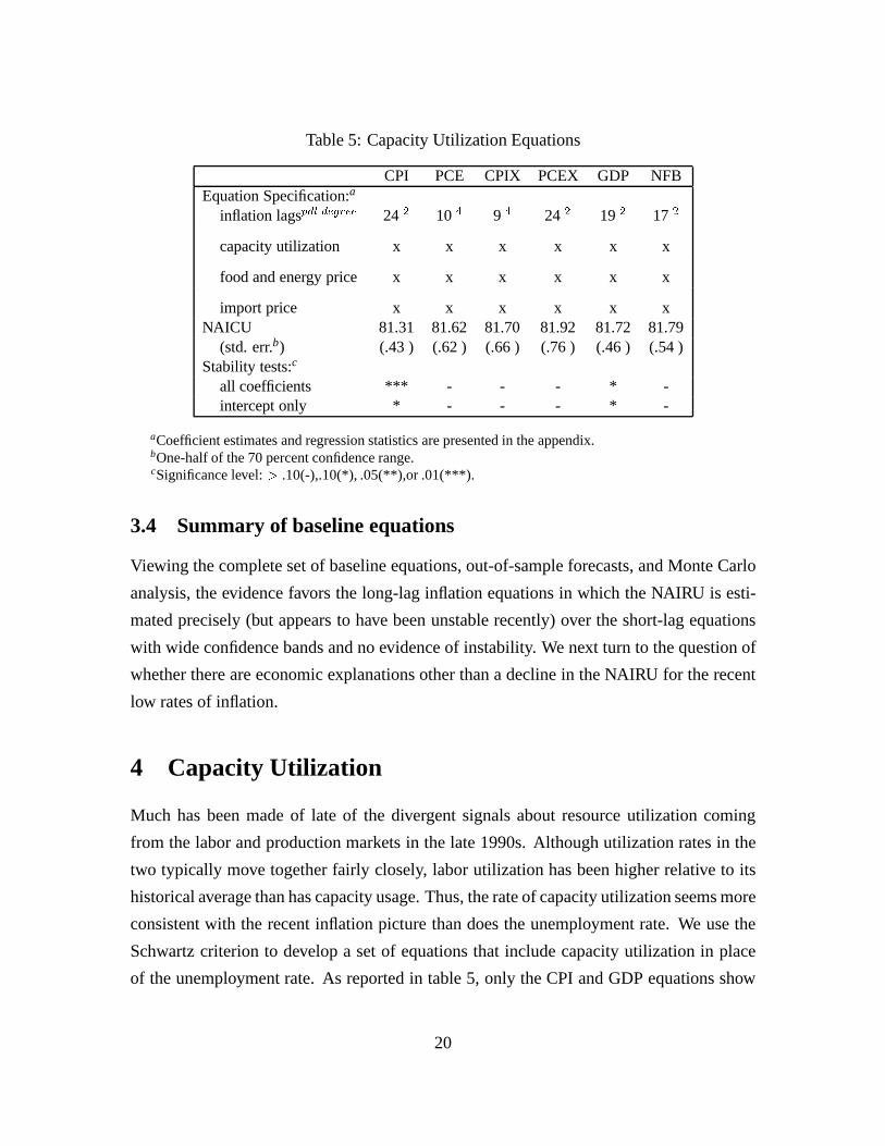
Table 5: Capacity Utilization Equations



capacity utilization x x x x x x


import price x x x x x xNAICU 81.31 81.62 81.70 81.92 81.72 81.79


all coefficients *** - - - * -intercept only * - - - * -

aCoefficient estimates and regression statistics are presented in the appendix.bOne-half of the 70 percent confidence range.cSignificance level:> .10(-),.10(*), .05(**),or .01(***).

3.4 Summary of baseline equations

Viewing the complete set of baseline equations, out-of-sample forecasts, and Monte Carlo

analysis, the evidence favors the long-lag inflation equations in which the NAIRU is esti-

mated precisely (but appears to have been unstable recently) over the short-lag equations

with wide confidence bands and no evidence of instability. We next turn to the question of

whether there are economic explanations other than a decline in the NAIRU for the recent

low rates of inflation.

4 Capacity Utilization

Much has been made of late of the divergent signals about resource utilization coming

from the labor and production markets in the late 1990s. Although utilization rates in the

two typically move together fairly closely, labor utilization has been higher relative to its

historical average than has capacity usage. Thus, the rate of capacity utilization seems more

consistent with the recent inflation picture than does the unemployment rate. We use the

Schwartz criterion to develop a set of equations that include capacity utilization in place

of the unemployment rate. As reported in table 5, only the CPI and GDP equations show

20

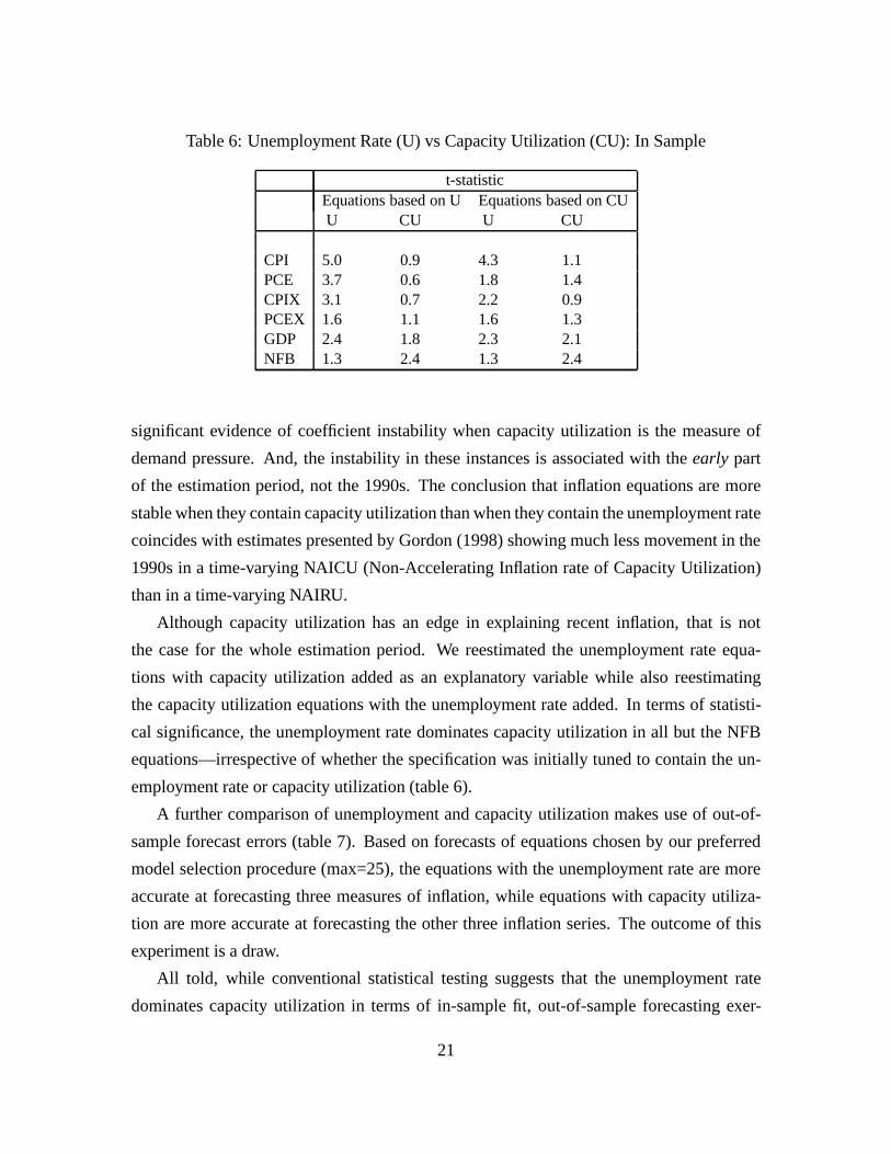
Table 6: Unemployment Rate (U) vs Capacity Utilization (CU): In Sample

t-statisticEquations based on U Equations based on CUU CU U CU

CPI 5.0 0.9 4.3 1.1PCE 3.7 0.6 1.8 1.4CPIX 3.1 0.7 2.2 0.9PCEX 1.6 1.1 1.6 1.3GDP 2.4 1.8 2.3 2.1NFB 1.3 2.4 1.3 2.4

significant evidence of coefficient instability when capacity utilization is the measure of

demand pressure. And, the instability in these instances is associated with theearly part

of the estimation period, not the 1990s. The conclusion that inflation equations are more

stable when they contain capacity utilization than when they contain the unemployment rate

coincides with estimates presented by Gordon (1998) showing much less movement in the

1990s in a time-varying NAICU (Non-Accelerating Inflation rate of Capacity Utilization)

than in a time-varying NAIRU.

Although capacity utilization has an edge in explaining recent inflation, that is not

the case for the whole estimation period. We reestimated the unemployment rate equa-

tions with capacity utilization added as an explanatory variable while also reestimating

the capacity utilization equations with the unemployment rate added. In terms of statisti-

cal significance, the unemployment rate dominates capacity utilization in all but the NFB

equations—irrespective of whether the specification was initially tuned to contain the un-

employment rate or capacity utilization (table 6).

A further comparison of unemployment and capacity utilization makes use of out-of-

sample forecast errors (table 7). Based on forecasts of equations chosen by our preferred

model selection procedure (max=25), the equations with the unemployment rate are more

accurate at forecasting three measures of inflation, while equations with capacity utiliza-

tion are more accurate at forecasting the other three inflation series. The outcome of this

experiment is a draw.

All told, while conventional statistical testing suggests that the unemployment rate

dominates capacity utilization in terms of in-sample fit, out-of-sample forecasting exer-

21

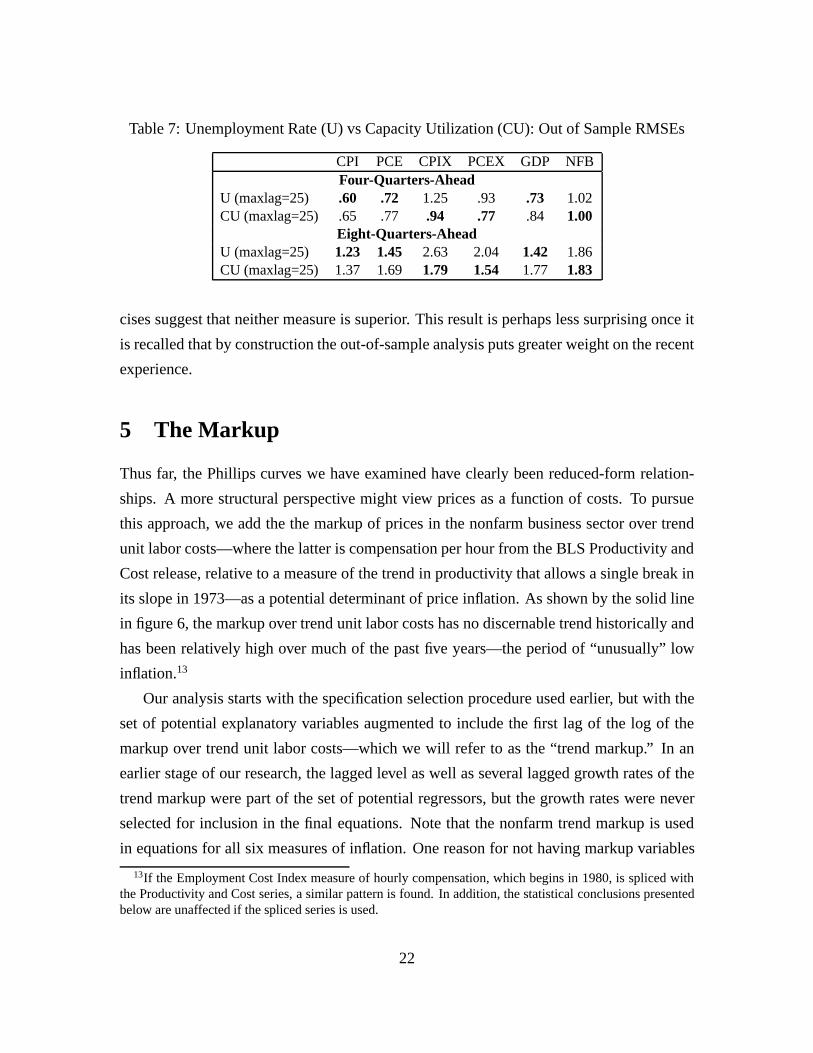
Table 7: Unemployment Rate (U) vs Capacity Utilization (CU): Out of Sample RMSEs

CPI PCE CPIX PCEX GDP NFBFour-Quarters-Ahead

U (maxlag=25) .60 .72 1.25 .93 .73 1.02CU (maxlag=25) .65 .77 .94 .77 .84 1.00

Eight-Quarters-AheadU (maxlag=25) 1.23 1.45 2.63 2.04 1.42 1.86CU (maxlag=25) 1.37 1.69 1.79 1.54 1.77 1.83

cises suggest that neither measure is superior. This result is perhaps less surprising once it

is recalled that by construction the out-of-sample analysis puts greater weight on the recent

experience.

5 The Markup

Thus far, the Phillips curves we have examined have clearly been reduced-form relation-

ships. A more structural perspective might view prices as a function of costs. To pursue

this approach, we add the the markup of prices in the nonfarm business sector over trend

unit labor costs—where the latter is compensation per hour from the BLS Productivity and

Cost release, relative to a measure of the trend in productivity that allows a single break in

its slope in 1973—as a potential determinant of price inflation. As shown by the solid line

in figure 6, the markup over trend unit labor costs has no discernable trend historically and

has been relatively high over much of the past five years—the period of “unusually” low

inflation.13

Our analysis starts with the specification selection procedure used earlier, but with the

set of potential explanatory variables augmented to include the first lag of the log of the

markup over trend unit labor costs—which we will refer to as the “trend markup.” In an

earlier stage of our research, the lagged level as well as several lagged growth rates of the

trend markup were part of the set of potential regressors, but the growth rates were never

selected for inclusion in the final equations. Note that the nonfarm trend markup is used

in equations for all six measures of inflation. One reason for not having markup variables

13If the Employment Cost Index measure of hourly compensation, which begins in 1980, is spliced withthe Productivity and Cost series, a similar pattern is found. In addition, the statistical conclusions presentedbelow are unaffected if the spliced series is used.

22

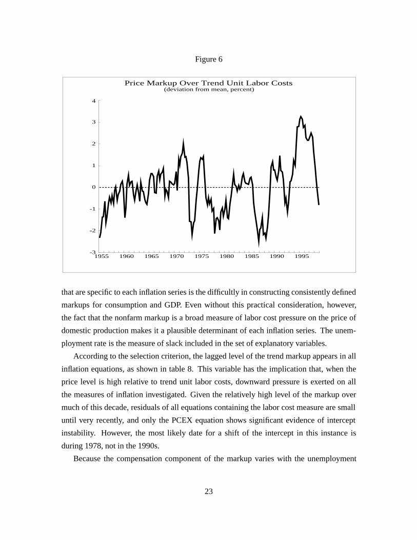
Figure 6

Price Markup Over Trend Unit Labor Costs(deviation from mean, percent)

1955 1960 1965 1970 1975 1980 1985 1990 1995-3

-2

-1

0

1

2

3

4

that are specific to each inflation series is the difficultly in constructing consistently defined

markups for consumption and GDP. Even without this practical consideration, however,

the fact that the nonfarm markup is a broad measure of labor cost pressure on the price of

domestic production makes it a plausible determinant of each inflation series. The unem-

ployment rate is the measure of slack included in the set of explanatory variables.

According to the selection criterion, the lagged level of the trend markup appears in all

inflation equations, as shown in table 8. This variable has the implication that, when the

price level is high relative to trend unit labor costs, downward pressure is exerted on all

the measures of inflation investigated. Given the relatively high level of the markup over

much of this decade, residuals of all equations containing the labor cost measure are small

until very recently, and only the PCEX equation shows significant evidence of intercept

instability. However, the most likely date for a shift of the intercept in this instance is

during 1978, not in the 1990s.

Because the compensation component of the markup varies with the unemployment

23

Table 8: Markup Equations





import price x x x

trend markup x x x x x xNAIRUb 5.97 5.88 6.05 6.01 5.88 5.84

(std. err.c) (.10 ) (.13 ) (.16 ) (.18 ) (.15 ) (.18 )Stability tests:d

all coefficients - - - - - -intercept only - - - * - -

aCoefficient estimates and regression statistics are presented in the appendix.bMeasured assuming the markup is at its sample mean.cOne-half of the 70 percent confidence range.dSignificance level:> .10(-),.10(*), .05(**),or .01(***).

rate, the NAIRU is not uniquely defined by the structure of equations for price inflation

when they contain the markup. Rather, such equations only pin down a linear relationship

between the NAIRU and the equilibrium value of the markup. Nonetheless, for illustrative

purposes, we report estimates of the NAIRU based on setting the markup to its sample

mean. As is shown in table 8, these estimates are close to 6 percent and are very similar to

the NAIRU values in the Baseline-98 equations.

The improvement in coefficient stability that characterizes the markup equations is

highlighted in figure 7, which contrasts Kalman filter estimates of time-varying NAIRUs

for the markup specifications with those shown earlier for the Baseline-98 equations.14

Indeed, for the CPIX markup equation, the median unbiased estimate of the variance of

innovations to the intercept is zero and its time-varying NAIRU is constant. And NAIRUs

in the CPI, PCE, GDP and NFB equations with the markup fall only 0.12 to 0.21 percent-

age points from 1989 to 1998. Only the PCEX equations exhibit similar movements of the

NAIRU over time in the markup and Baseline-98 specifications.

14The characteristics of figure 7 would be unchanged if estimates of time-varying intercepts were shownrather than time-varying NAIRUs.

24

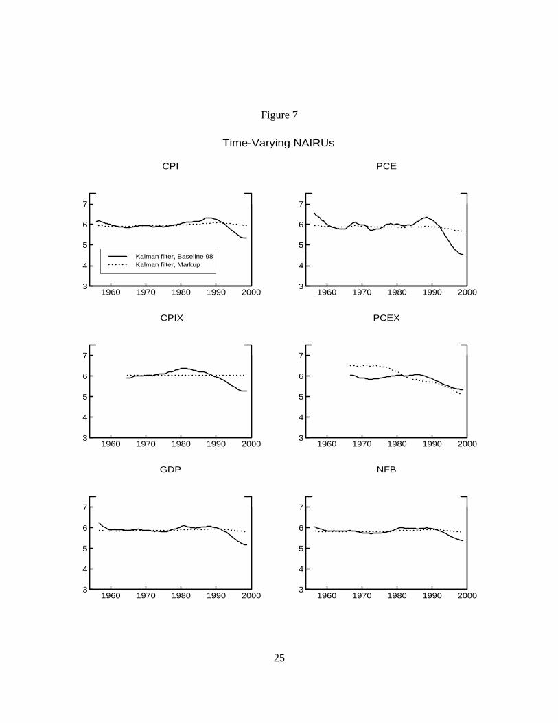
Figure 7

3

4

5

6

7

1960 1970 1980 1990 2000

CPI

Kalman filter, Baseline 98Kalman filter, Markup

3

4

5

6

7

1960 1970 1980 1990 2000

PCE

3

4

5

6

7

1960 1970 1980 1990 2000

CPIX

3

4

5

6

7

1960 1970 1980 1990 2000

PCEX

3

4

5

6

7

1960 1970 1980 1990 2000

GDP

3

4

5

6

7

1960 1970 1980 1990 2000

NFB

Time-Varying NAIRUs

25

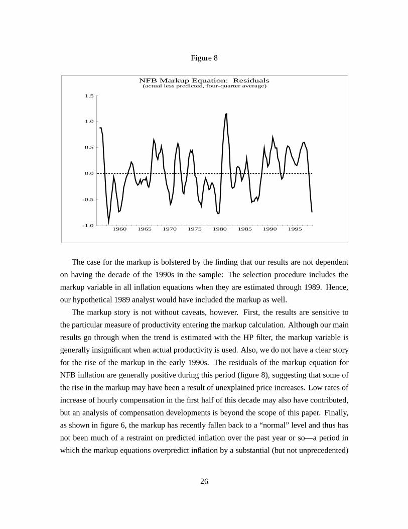
Figure 8

NFB Markup Equation: Residuals(actual less predicted, four-quarter average)

1960 1965 1970 1975 1980 1985 1990 1995-1.0

-0.5

0.0

0.5

1.0

1.5

The case for the markup is bolstered by the finding that our results are not dependent

on having the decade of the 1990s in the sample: The selection procedure includes the

markup variable in all inflation equations when they are estimated through 1989. Hence,

our hypothetical 1989 analyst would have included the markup as well.

The markup story is not without caveats, however. First, the results are sensitive to

the particular measure of productivity entering the markup calculation. Although our main

results go through when the trend is estimated with the HP filter, the markup variable is

generally insignificant when actual productivity is used. Also, we do not have a clear story

for the rise of the markup in the early 1990s. The residuals of the markup equation for

NFB inflation are generally positive during this period (figure 8), suggesting that some of

the rise in the markup may have been a result of unexplained price increases. Low rates of

increase of hourly compensation in the first half of this decade may also have contributed,

but an analysis of compensation developments is beyond the scope of this paper. Finally,

as shown in figure 6, the markup has recently fallen back to a “normal” level and thus has

not been much of a restraint on predicted inflation over the past year or so—a period in

which the markup equations overpredict inflation by a substantial (but not unprecedented)

26

amount (figure 8). Because the overprediction episode is as yet fairly short, it is too soon to

say whether the errors are transitory or evidence of some other factor restraining inflation.

One possible restraint on recent inflation not captured in our markup equations would

be a pickup in the trend rate of growth of labor productivity. If this were the case, the

level of the trend markup might be higher than our measure, reducing the predicted rate

of inflation. Much speculation has arisen concerning possible effects of booming invest-

ment in computers and related equipment on labor productivity, but as yet no consensus

has emerged. And in one study pointing to an increase in the trend rate of growth of la-

bor productivity in the nonfarm sector, the level of the trend is only slightly above our

measure—based on the single kink at 1973—at the end of 1998, and thus would not have

substantially different implications for inflation.15

6 Conclusions

The baseline version of the Phillips curve cannot adequately explain why inflation has been

so low in the second half of the 1990s. While import prices, which are part of the baseline

specification, are estimated in most equations to have restrained inflation over the past few

years, a full attribution of inflation developments to these prices would require a many-fold

increase in their coefficients. Looking beyond the baseline framework, capacity utilization

predicts inflation in the recent period more accurately than does the unemployment rate, but

the reverse tends to hold for the estimation sample as a whole on an in-sample basis. Out-

of-sample forecast accuracy provides no basis for discriminating between the two measures

of utilization.

We find that evidence favors a view in which price developments are, in part, deter-

mined by an “error-correction” mechanism involving the markup of prices over trend unit

labor costs. A high markup puts downward pressure on price inflation and the reverse ob-

tains when the markup is low. With markups relatively high through much of the 1990s, the

error-correction channel is estimated to have held down inflation over much of this period.

The reason for the past rise in the markup is somewhat unclear. However, markup levels at

the end of 1998 are close to their historical averages and thus should not restrain inflation in

the near future, unless, for some reason, firms are under pressure to reduce margins below

15Gordon (1999). We adjust Gordon's estimate of trend productivity growth to be consistent with ourassumption about the effect of changes in price measurement methods on labor productivity.

27

historical norms or trend labor productivity is rising faster than our simple calculation.

Additional support for the markup story comes from the observation that not only does

it have a long history as a theoretical model of price determination but also that we find it

empirically to be a stable part of inflation dynamics over time. The markup is an explana-

tion of what has happened to inflation this decade that could have been identified as part of

the inflation process prior to this decade.

28

References

Andrews, Donald, Inpyo Lee, and Werner Ploberger (1996) Optimal Changepoint Tests

for Normal Linear Regression.Journal of Econometrics, 70, 9-38.

Andrews, Donald, and Werner Ploberger (1994) Optimal Tests When a Nuisance Pa-

rameter is Present Only Under the Alternative.Econometrica, 62, 1383-1414.

Council of Economic Advisors (1999)Economic Report of the President. Washington

D.C.: United States Government Printing Office.

Fuhrer, Jeffrey C. (1995) The Phillips Curve is Alive and Well.New England Economic

Review of the Federal Reserve Bank of Boston, March/April, 41-56.

Gordon, Robert J. (1997) The Time-Varying NAIRU and its Implications for Economic

Policy. Journal of Economic Perspectives, 11, 11-32.

Gordon, Robert J. (1998) Foundations of the Goldilocks Economy: Supply Shocks and

the Time-Varying NAIRU.Brookings Papers on Economic Activity, 297-333.

Gordon, Robert J. (1999) Has the ' New Economy' Rendered the Productivity Slow-

down Obsolete? Northwestern University, mimeo.

Katz, Lawrence F., and Alan B. Krueger (1999) The High-Pressure U.S. Labor Market

of the 1990s.Brookings Papers on Economic Activity, forthcoming.

McIntire, Robert J. (1996) Revisions in Household Survey Data Effective February

1996.Employment and Earnings, March, 8-16.

Polivka, Anne E., and Stephen M. Miller (1995) The CPS After the Redesign: Refo-

cusing the Economic Lens. Bureau of Labor Statistics, Mimeo, March.

29

Staiger, Douglas, James H. Stock, and Mark W. Watson (1997a) How Precise Are Esti-

mates of the Natural Rate of Unemployment?Reducing Inflation: Motivation and Strategy,

ed. Christina D. Romer and David H. Romer. University of Chicago Press.

Staiger, Douglas, James H. Stock, and Mark W. Watson (1997b) The NAIRU, Unem-

ployment and Monetary PolicyJournal of Economic Perspectives, 11, 33-49.

Stock, James H., and Mark W. Watson (1998) Median Unbiased Estimation of Coef-

ficient Variance in a Time-Varying Parameter Model.Journal of the American Statistical

Association, 93, 349-58.

Stock, James H., and Mark W. Watson (1999) Forecasting Inflation. NBER working

paper 7023.

Tootell, Geoffrey (1994) Restructuring, the NAIRU, and the Phillips Curve.New Eng-

land Economic Review of the Federal Reserve Bank of Boston, September/October, 31-44.

30

Appendix Tables

Table A1Baseline-89 Equations

CPI PCE CPIX PCEX GDP NFBEstimated coefficients:a

inflation lagsb 1.0021;25 1.002

1;24 1.0021;24 1.002

1;24 1.0021;19 1.002

1;17

(0.5 ) (0.1 ) (1.9 ) (0.1 ) (0.9 ) (0.1 )

unemployment rate -.54 -.4500;1 -.37 -.3600;3 -.47 00;1 -.480

0;1

(11.7 ) (8.9 ) (7.5 ) (6.2 ) (8.0 ) (7.0 )

food and energy price .89 .94 .50 .57(contemporaneous) (21.4 ) (15.2 ) (6.1 ) (6.3 )

food and energy price .4501;4 .5001;3 -.21 1;1

(lags) (7.5 ) (5.7 ) (2.6 )

farm price -.02(8.1 )

import price .03 .0700;3 .1100;3

(2.8 ) (4.5 ) (5.9 )Equation statistics:

sample period 55.1 - 89.4 55.1 - 89.4 63.3 - 89.4 65.3 - 89.4 55.1 - 89.4 55.1 - 89.4�R2 .9410 .9320 .8903 .8565 .9042 .8934

SSR 74.48 73.37 57.12 56.44 92.14 137.53regression se .7455 .7427 .7557 .7832 .8355 1.0207Durbin-Watson 1.81 1.61 1.80 1.52 1.83 1.84

aFor each regressor, the estimated coefficient, or coefficient sum, and t-statistic are reported. Entries thatare coefficient sums are indicated by subscripts indexing the minimum and maximum lags, and, if polynomialrestrictions are imposed, by a superscript reporting the polynomial degree. Equations also include an interceptand wage-price dummy.

bThe reported t-statistic is associated with the deviation from one of the sum of coefficients on laggedinflation when it is not restricted.

31

Table A2Baseline-98 Equations



1;24 1.0021;23 1.002

1;24 1.0021;15 1.002

1;17

(0.1 ) (0.2 ) (2.3 ) (0.2 ) (0.0 ) (0.2 )

unemployment rate -.5000;1 -.4000;1 -.35 -.2700;3 -.37 -.4100;1

(11.3 ) (8.3 ) (8.0 ) (5.0 ) (6.8 ) (6.3 )


food and energy price .4501;4 .360

1;3

(lags) (8.2 ) (3.8 )


import price .0400;1 .0400;1 .05 1

0;1 .1100;2

(3.8 ) (3.3 ) (3.8 ) (6.9 )Equation statistics:

sample period 55.1 - 98.4 55.1 - 98.4 63.3 - 98.4 65.3 - 98.4 55.1 - 98.4 55.1 - 98.4�R2 .9350 .9223 .8909 .8796 .8962 .8845

SSR 89.48 94.48 68.80 71.51 114.73 166.58regression se .7255 .7477 .7112 .7504 .8264 .9958Durbin-Watson 1.66 1.51 1.74 1.53 1.76 1.74



32

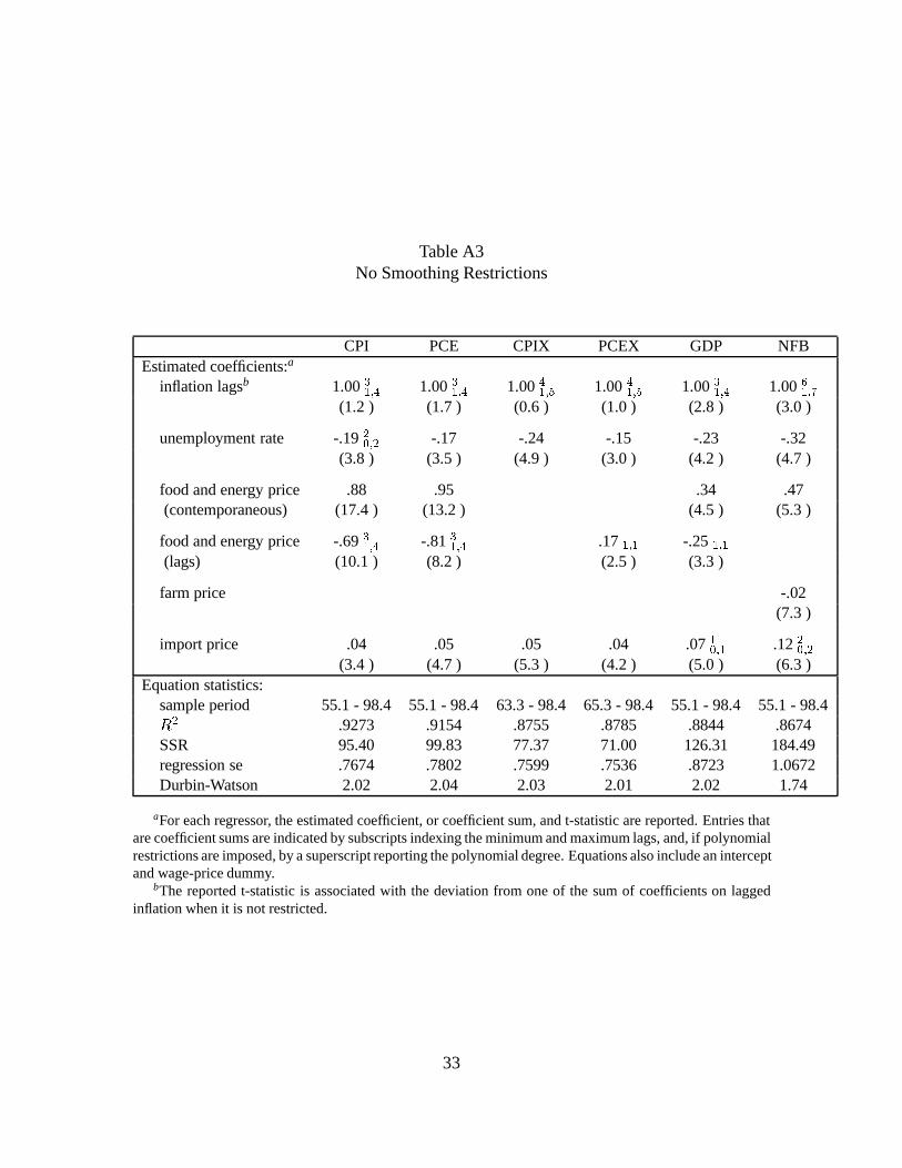
Table A3No Smoothing Restrictions



1;4 1.0041;5 1.004

1;5 1.0031;4 1.006

1;7

(1.2 ) (1.7 ) (0.6 ) (1.0 ) (2.8 ) (3.0 )

unemployment rate -.1920;2 -.17 -.24 -.15 -.23 -.32

(3.8 ) (3.5 ) (4.9 ) (3.0 ) (4.2 ) (4.7 )


food and energy price -.6931;4 -.8131;4 .171;1 -.25 1;1

(lags) (10.1 ) (8.2 ) (2.5 ) (3.3 )


import price .04 .05 .05 .04 .0710;1 .1220;2

(3.4 ) (4.7 ) (5.3 ) (4.2 ) (5.0 ) (6.3 )Equation statistics:

sample period 55.1 - 98.4 55.1 - 98.4 63.3 - 98.4 65.3 - 98.4 55.1 - 98.4 55.1 - 98.4�R2 .9273 .9154 .8755 .8785 .8844 .8674

SSR 95.40 99.83 77.37 71.00 126.31 184.49regression se .7674 .7802 .7599 .7536 .8723 1.0672Durbin-Watson 2.02 2.04 2.03 2.01 2.02 1.74



33

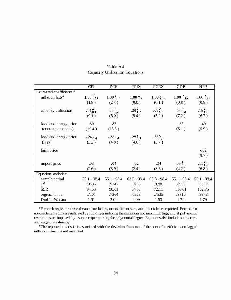
Table A4Capacity Utilization Equations



1;10 1.0041;9 1.002

1;24 1.0021;19 1.002

1;17

(1.8 ) (2.4 ) (0.0 ) (0.1 ) (0.8 ) (0.8 )

capacity utilization .1400;1 .0900;3 .09 0

0;3 .0900;3 .14 0

0;3 .1500;3

(9.1 ) (5.0 ) (5.4 ) (5.2 ) (7.2 ) (6.7 )


food and energy price -.2401;4 -.381;1 .28 0

1;4 .3601;4

(lags) (3.2 ) (4.8 ) (4.0 ) (3.7 )


import price .03 .04 .02 .04 .0510;1 .1100;2


sample period 55.1 - 98.4 55.1 - 98.4 63.3 - 98.4 65.3 - 98.4 55.1 - 98.4 55.1 - 98.4�R2 .9305 .9247 .8953 .8786 .8950 .8872




34

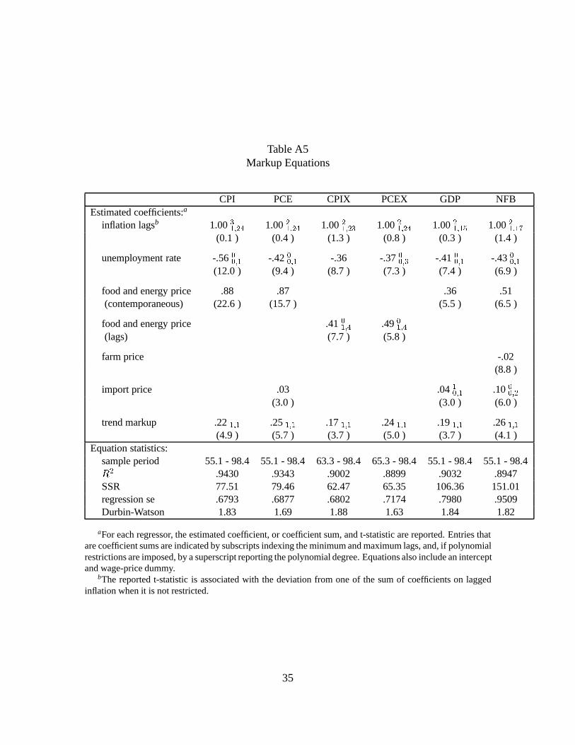
Table A5Markup Equations



1;24 1.0021;23 1.002

1;24 1.0021;15 1.002

1;17

(0.1 ) (0.4 ) (1.3 ) (0.8 ) (0.3 ) (1.4 )

unemployment rate -.5600;1 -.420

0;1 -.36 -.3700;3 -.41 0

0;1 -.4300;1

(12.0 ) (9.4 ) (8.7 ) (7.3 ) (7.4 ) (6.9 )


food and energy price .4101;4 .4901;4

(lags) (7.7 ) (5.8 )


import price .03 .0410;1 .1000;2

(3.0 ) (3.0 ) (6.0 )

trend markup .221;1 .251;1 .17 1;1 .241;1 .19 1;1 .261;1


sample period 55.1 - 98.4 55.1 - 98.4 63.3 - 98.4 65.3 - 98.4 55.1 - 98.4 55.1 - 98.4�R2 .9430 .9343 .9002 .8899 .9032 .8947




35

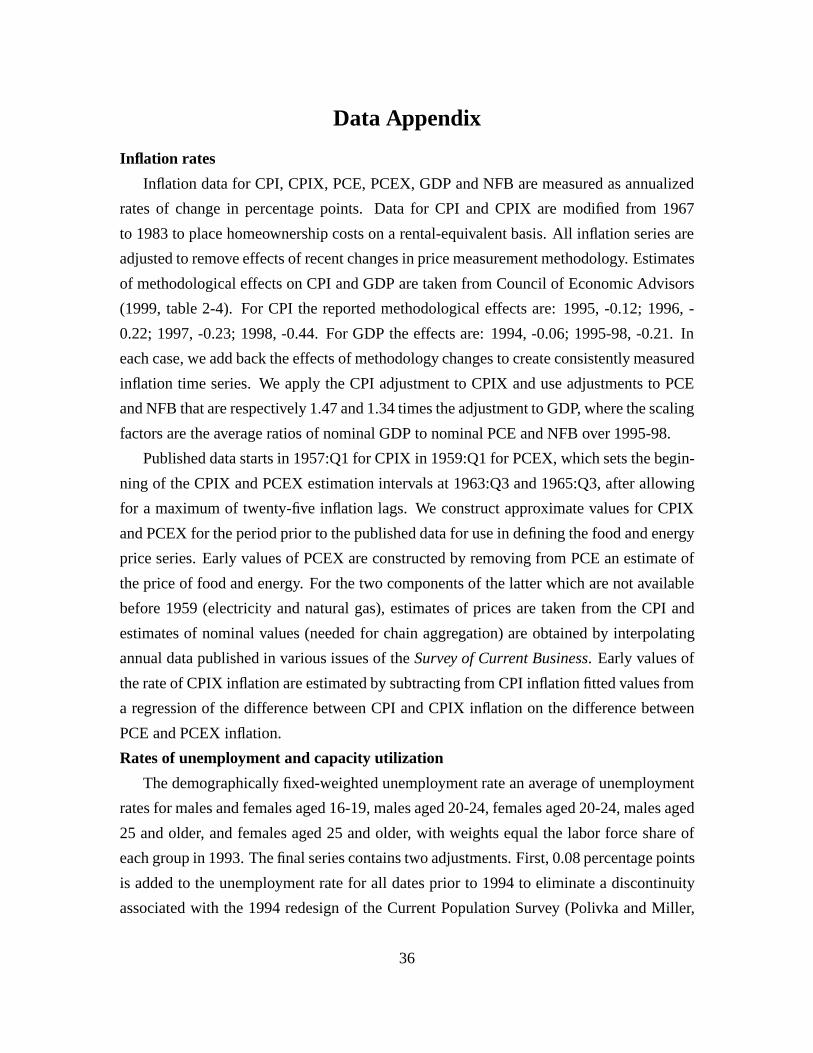
Data Appendix

Inflation rates

Inflation data for CPI, CPIX, PCE, PCEX, GDP and NFB are measured as annualized

rates of change in percentage points. Data for CPI and CPIX are modified from 1967

to 1983 to place homeownership costs on a rental-equivalent basis. All inflation series are

adjusted to remove effects of recent changes in price measurement methodology. Estimates

of methodological effects on CPI and GDP are taken from Council of Economic Advisors

(1999, table 2-4). For CPI the reported methodological effects are: 1995, -0.12; 1996, -

0.22; 1997, -0.23; 1998, -0.44. For GDP the effects are: 1994, -0.06; 1995-98, -0.21. In

each case, we add back the effects of methodology changes to create consistently measured

inflation time series. We apply the CPI adjustment to CPIX and use adjustments to PCE

and NFB that are respectively 1.47 and 1.34 times the adjustment to GDP, where the scaling

factors are the average ratios of nominal GDP to nominal PCE and NFB over 1995-98.

Published data starts in 1957:Q1 for CPIX in 1959:Q1 for PCEX, which sets the begin-

ning of the CPIX and PCEX estimation intervals at 1963:Q3 and 1965:Q3, after allowing

for a maximum of twenty-five inflation lags. We construct approximate values for CPIX

and PCEX for the period prior to the published data for use in defining the food and energy

price series. Early values of PCEX are constructed by removing from PCE an estimate of

the price of food and energy. For the two components of the latter which are not available

before 1959 (electricity and natural gas), estimates of prices are taken from the CPI and

estimates of nominal values (needed for chain aggregation) are obtained by interpolating

annual data published in various issues of theSurvey of Current Business. Early values of

the rate of CPIX inflation are estimated by subtracting from CPI inflation fitted values from

a regression of the difference between CPI and CPIX inflation on the difference between

PCE and PCEX inflation.

Rates of unemployment and capacity utilization

The demographically fixed-weighted unemployment rate an average of unemployment

rates for males and females aged 16-19, males aged 20-24, females aged 20-24, males aged

25 and older, and females aged 25 and older, with weights equal the labor force share of

each group in 1993. The final series contains two adjustments. First, 0.08 percentage points

is added to the unemployment rate for all dates prior to 1994 to eliminate a discontinuity

associated with the 1994 redesign of the Current Population Survey (Polivka and Miller,

36

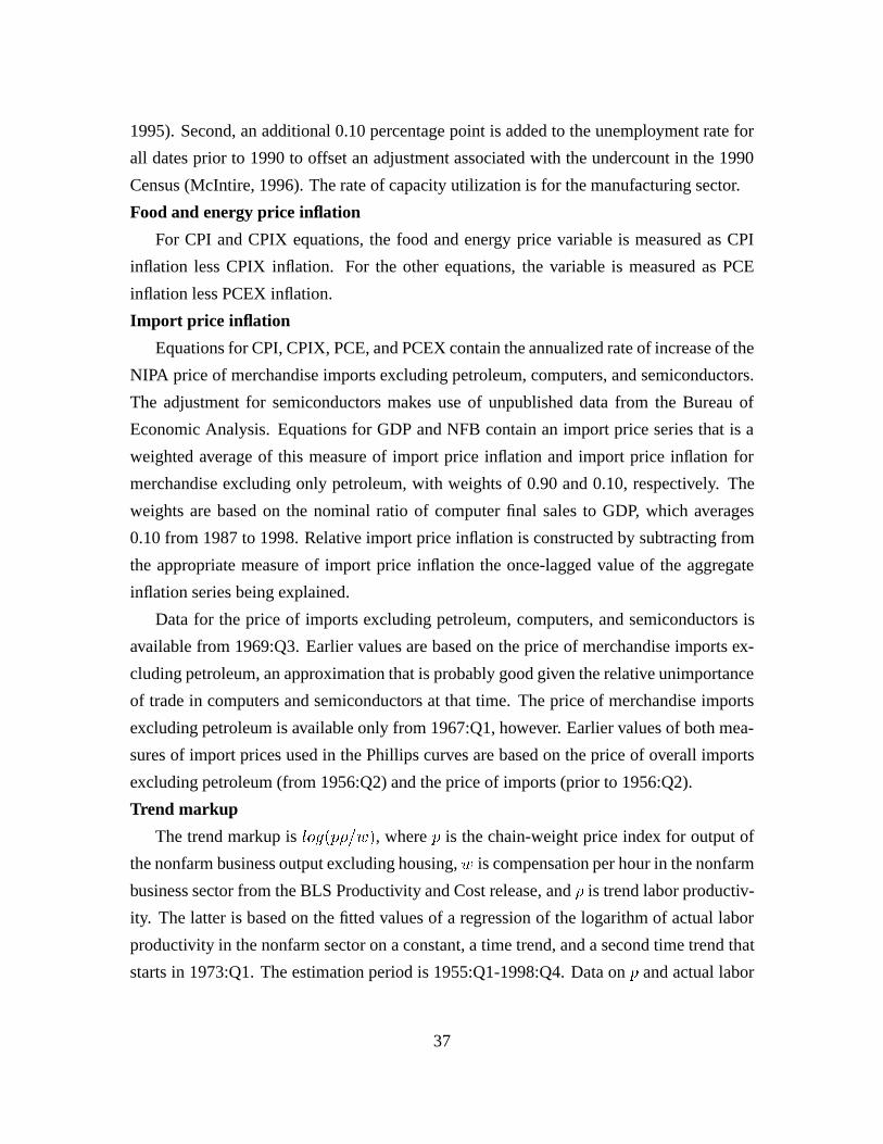
1995). Second, an additional 0.10 percentage point is added to the unemployment rate for

all dates prior to 1990 to offset an adjustment associated with the undercount in the 1990

Census (McIntire, 1996). The rate of capacity utilization is for the manufacturing sector.

Food and energy price inflation

For CPI and CPIX equations, the food and energy price variable is measured as CPI

inflation less CPIX inflation. For the other equations, the variable is measured as PCE

inflation less PCEX inflation.

Import price inflation

Equations for CPI, CPIX, PCE, and PCEX contain the annualized rate of increase of the

NIPA price of merchandise imports excluding petroleum, computers, and semiconductors.

The adjustment for semiconductors makes use of unpublished data from the Bureau of

Economic Analysis. Equations for GDP and NFB contain an import price series that is a

weighted average of this measure of import price inflation and import price inflation for

merchandise excluding only petroleum, with weights of 0.90 and 0.10, respectively. The

weights are based on the nominal ratio of computer final sales to GDP, which averages

0.10 from 1987 to 1998. Relative import price inflation is constructed by subtracting from

the appropriate measure of import price inflation the once-lagged value of the aggregate

inflation series being explained.

Data for the price of imports excluding petroleum, computers, and semiconductors is

available from 1969:Q3. Earlier values are based on the price of merchandise imports ex-

cluding petroleum, an approximation that is probably good given the relative unimportance

of trade in computers and semiconductors at that time. The price of merchandise imports

excluding petroleum is available only from 1967:Q1, however. Earlier values of both mea-

sures of import prices used in the Phillips curves are based on the price of overall imports

excluding petroleum (from 1956:Q2) and the price of imports (prior to 1956:Q2).

Trend markup

The trend markup islog(p�=w), wherep is the chain-weight price index for output of

the nonfarm business output excluding housing,w is compensation per hour in the nonfarm

business sector from the BLS Productivity and Cost release, and� is trend labor productiv-

ity. The latter is based on the fitted values of a regression of the logarithm of actual labor

productivity in the nonfarm sector on a constant, a time trend, and a second time trend that

starts in 1973:Q1. The estimation period is 1955:Q1-1998:Q4. Data onp and actual labor

37

productivity are adjusted for changes in price measurement methodology by cumulating

over time the adjustment to NFB inflation described above. The trend markup is measured

relative to its 1955-98 mean.

Wage-price control variable

All equations contain a variable that accounts for the effects of wage and price controls

in the 1970s. The series, which has a mean of zero, equals 1.0 from 1971:Q3 to 1974:Q1

and -3.67 from 1974:Q2-1974:Q4.

38

Documents

What's Happened to the Phillips Curve? - Federal …s Happened to the Phillips Curve? Flint Brayton, John M. Roberts, and John C. Williams Division of Research and Statistics Federal