Embed Size (px)
Citation preview

What’s New in Econometrics?Lecture 2
Linear Panel Data Models
Jeff WooldridgeNBER Summer Institute, 2007
1. Overview of the Basic Model
2. New Insights Into Old Estimators
3. Behavior of Estimators without Strict Exogeneity
4. IV Estimation under Sequential Exogeneity
5. Pseudo Panels from Pooled Cross Sections
1
1. Overview of the Basic Model
∙ Unless stated otherwise, the methods discussed in
these slides are for the case with a large cross
section and small time series.
∙ For a generic i in the population,
yit t xit ci uit, t 1, . . . ,T, (1)
where t is a separate time period intercept, xit is a
1 K vector of explanatory variables, ci is the
time-constant unobserved effect, and the
uit : t 1, . . . ,T are idiosyncratic errors. We
view the ci as random draws along with the
observed variables.
∙ An attractive assumption is contemporaneous
exogeneity conditional on ci :
Euit|xit,ci 0, t 1, . . . ,T. (2)
2
This equation defines in the sense that under (1)
and (2),
Eyit|xit,ci t xit ci, (3)
so the j are partial effects holding ci fixed.
∙ Unfortunately, is not identified only under (2).
If we add the strong assumption Covxit,ci 0,
then is identified.
∙ Allow any correlation between xit and ci by
assuming strict exogeneity conditional on ci :
Euit|xi1,xi2, . . . ,xiT,ci 0, t 1, . . . ,T, (4)
which can be expressed as
Eyit|xi,ci Eyit|xit,ci t xit ci. (5)
If xit : t 1, . . . ,T has suitable time variation,
can be consistently estimated by fixed effects (FE)
or first differencing (FD), or generalized least
3

squares (GLS) or generalized method of moments
(GMM) versions of them.
∙Make inference fully robust to heteroksedasticity
and serial dependence, even if use GLS. With large
N and small T, there is little excuse not to compute
“cluster” standard errors.
∙ Violation of strict exogeneity: always if xit
contains lagged dependent variables, but also if
changes in uit cause changes in xi,t1 (“feedback
effect”).
∙ Sequential exogeneity condition on ci:
Euit|xi1,xi2, . . . ,xit,ci 0, t 1, . . . ,T (6)
or, maintaining the linear model,
Eyit|xi1, . . . ,xit,ci Eyit|xit,ci. (7)
Allows for lagged dependent variables and other
4
feedback. Generally, is identified under
sequential exogeneity. (More later.)
∙ The key “random effects” assumption is
Eci|xi Eci. (8)
Pooled OLS or any GLS procedure, including the
RE estimator, are consistent. Fully robust inference
is available for both.
∙ It is useful to define two correlated random
effects assumptions. The first just defines a linear
projection:
Lci|xi xi, (9)
Called the Chamberlain device, after Chamberlain
(1982). Mundlak (1978) used a restricted version
Eci|xi xi, (10)
where xi T−1∑t1T xit. Then
5

yit t xit xi ai uit, (11)
and we can apple pooled OLS or RE because
Eai uit|xi 0. Both equal the FE estimator of
.
∙ Equation (11) makes it easy to compute a fully
robust Hausman test comparing RE and FE.
Separate covariates into aggregate time effects,
time-constant variables, and variables that change
across i and t:
yit gt zi wit ci uit. (12)
We cannot estimate by FE, so it is not part of the
Hausman test comparing RE and FE. Less clear is
that coefficients on the time dummies, , cannot be
included, either. (RE and FE estimation only with
aggregate time effects are identical.) We can only
6

compare FE and RE M parameters).
∙ Convenient test:
yit on gt, zi, wit, wi, t 1, . . . ,T; i 1, . . . ,N, (13)
which makes it clear there are M restrictions to test.
Pooled OLS or RE, fully robust!
∙Must be cautious using canned procedures, as the
df are often wrong and tests nonrobust.
2. New Insights Into Old Estimators
∙ Consider an extension of the usual model to
allow for unit-specific slopes,
yit ci xitbi uit
Euit|xi,ci,bi 0, t 1, . . . ,T, (14) (15)
where bi is K 1. We act as if bi is constant for all
i but think ci might be correlated with xit; we apply
usual FE estimator. When does the usual FE
7

estimator consistently estimate the population
average effect, Ebi?
∙ A sufficient condition for consistency of the FE
estimator, along with along with (15) and the usual
rank condition, is
Ebi|xit Ebi , t 1, . . . ,T (16)
where xit are the time-demeaned covariates. Allows
the slopes, bi, to be correlated with the regressors
xit through permanent components. For example, if
xit f i rit, t 1, . . . ,T. Then (16) holds if
Ebi|ri1,ri2, . . . ,riT Ebi.
∙ Extends to a more general class of estimators.
Write
yit wtai xitbi uit, t 1, . . . ,T (17)
where wt is a set of deterministic functions of time.
8

FE now sweeps away ai by netting out wt from xit.
∙ In the random trend model, wt 1, t. If
xit f i hit rit, then bi can be arbitrarily
correlated with f i,hi.
∙ Generally, need dimwt T)
∙ Can apply to models with time-varying factor
loads, t :
yit xit tci uit, t 1, . . . ,T. (18)
Sufficient for consistency of FE estimator that
ignores the t is
Covxit,ci 0, t 1, . . . ,T. (19)
∙ Now let some elements of xit be correlated with
uir : r 1, . . . ,T, but with strictly exogenous
instruments (conditional on ci. Assume
Euit|zi,ai,bi 0 (20)
9

for all t. Also, replace (16) with
Ebi|zit Ebi , t 1, . . . ,T. (21)
Still not enough. A sufficient condition is
Covxit,bi|zit Covxit,bi, t 1, . . . ,T. (22)
Covxit,bi, a K K matrix, need not be zero, or
even constant across time. The conditional
covariance cannot depend on the time-demeaned
instruments. Then, FEIV is consistent for Ebi
provided a full set of time dummies is included.
∙ Assumption (22) cannot be expected to hold
when endogenous elements of xit are discrete.
3. Behavior of Estimators without Strict
Exogeneity
∙ Both the FE and FD estimators are inconsistent
(with fixed T, N → ) without the conditional strict
10
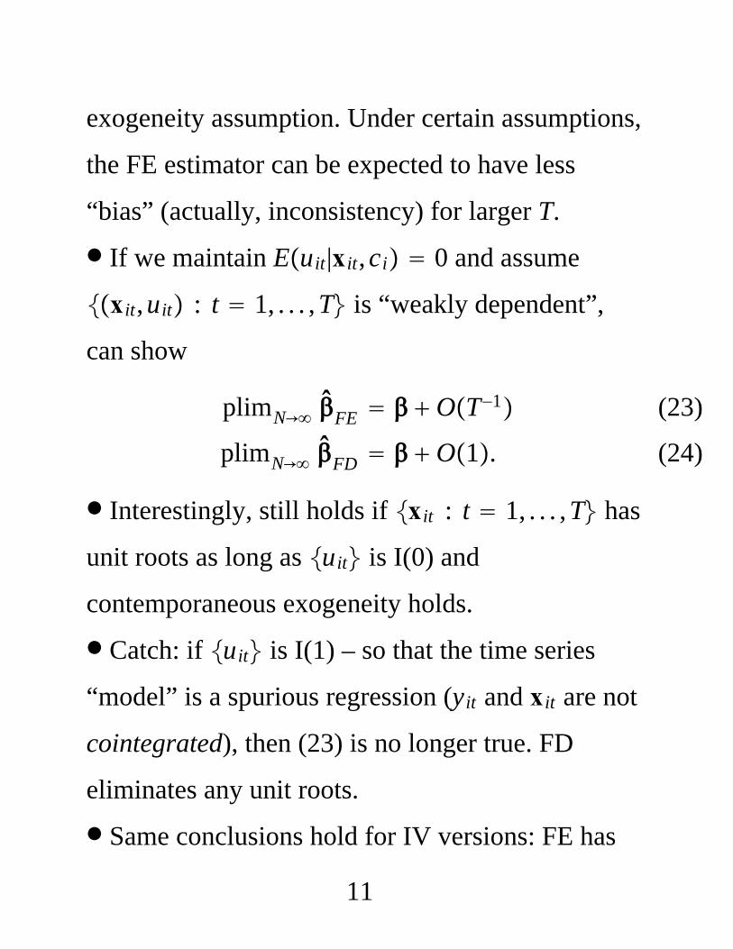
exogeneity assumption. Under certain assumptions,
the FE estimator can be expected to have less
“bias” (actually, inconsistency) for larger T.
∙ If we maintain Euit|xit,ci 0 and assume
xit,uit : t 1, . . . ,T is “weakly dependent”,
can show
plimN→ FE OT−1
plimN→ FD O1.
(23)
(24)
∙ Interestingly, still holds if xit : t 1, . . . ,T has
unit roots as long as uit is I(0) and
contemporaneous exogeneity holds.
∙ Catch: if uit is I(1) – so that the time series
“model” is a spurious regression (yit and xit are not
cointegrated), then (23) is no longer true. FD
eliminates any unit roots.
∙ Same conclusions hold for IV versions: FE has
11
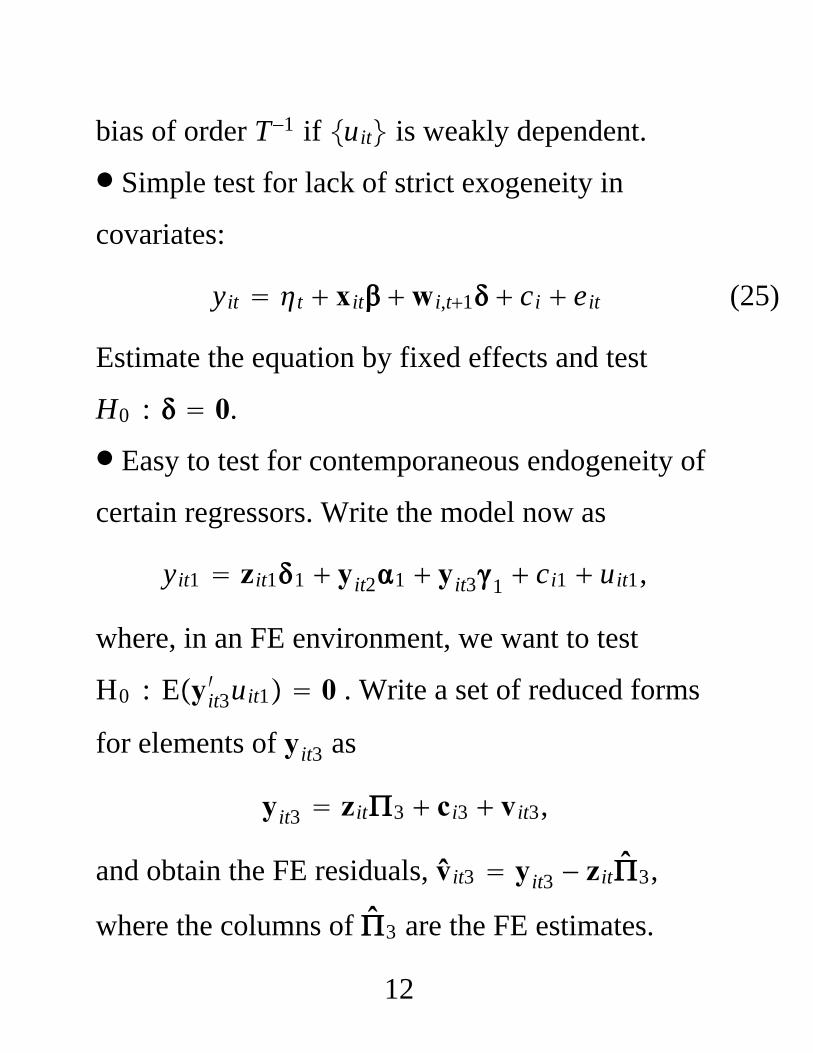
bias of order T−1 if uit is weakly dependent.
∙ Simple test for lack of strict exogeneity in
covariates:
yit t xit wi,t1 ci eit (25)
Estimate the equation by fixed effects and test
H0 : 0.
∙ Easy to test for contemporaneous endogeneity of
certain regressors. Write the model now as
yit1 zit11 yit21 yit31 ci1 uit1,
where, in an FE environment, we want to test
H0 : Eyit3′ uit1 0 . Write a set of reduced forms
for elements of yit3 as
yit3 zit3 ci3 vit3,
and obtain the FE residuals, vit3 yit3 − zit3,
where the columns of 3 are the FE estimates.
12

Then, estimate
yit1 zit11 yit21 yit31 vit31 errorit1
by FEIV, using instruments zit,yit3, vit3. The test
that yit3 is exogenous is just the (robust) test that
1 0, and the test need not adjust for the first-step
estimation.
4. IV Estimation under Sequential Exogeneity
We now consider IV estimation of the model
yit xit ci uit, t 1, . . . ,T, (26)
under sequential exogeneity assumptions; the
weakest form is Covxis,uit 0, all s ≤ t.
This leads to simple moment conditions after first
differencing:
Exis′ Δuit 0, s 1, . . . , t − 1; t 2, . . . ,T. (27)
Therefore, at time t, the available instruments in the
13

FD equation are in the vector
xito ≡ xi1,xi2, . . . ,xit. The matrix of instruments is
Wi diagxi1o ,xi2
o , . . . ,xi,T−1o , (28)
which has T − 1 rows. Routine to apply GMM
estimation.
∙ Simple strategy: estimate a reduced form for Δxit
separately for each t. So, at time t, run the
regression Δxit on xi,t−1o , i 1, . . . ,N, and obtain the
fitted values, Δxit. Then, estimate the FD equation
Δyit Δxit Δuit, t 2, . . . ,T (29)
by pooled IV using instruments (not regressors)
Δxit.
∙ Can suffer from a weak instrument problem when
Δxit has little correlation with xi,t−1o .
∙ If we assume
14
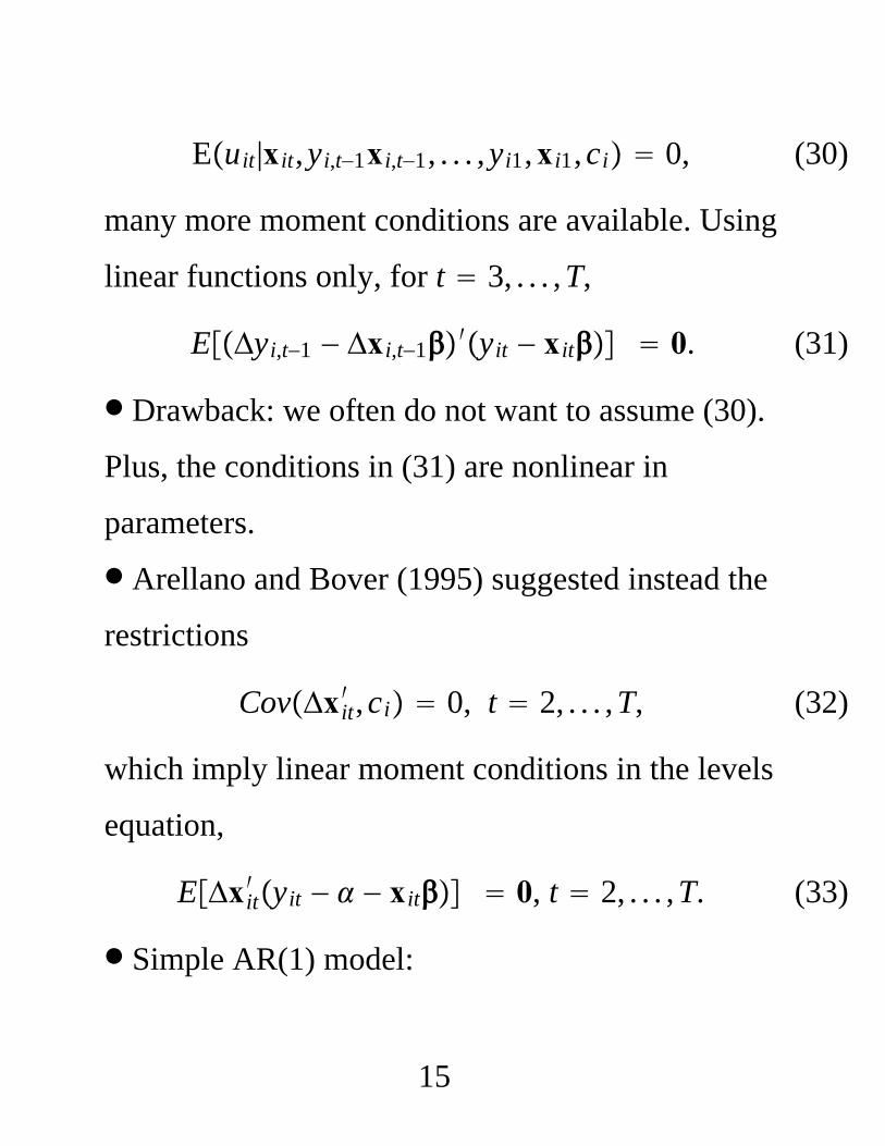
Euit|xit,yi,t−1xi,t−1, . . . ,yi1,xi1,ci 0, (30)
many more moment conditions are available. Using
linear functions only, for t 3, . . . ,T,
EΔyi,t−1 − Δxi,t−1′yit − xit 0. (31)
∙ Drawback: we often do not want to assume (30).
Plus, the conditions in (31) are nonlinear in
parameters.
∙ Arellano and Bover (1995) suggested instead the
restrictions
CovΔxit′ ,ci 0, t 2, . . . ,T, (32)
which imply linear moment conditions in the levels
equation,
EΔxit′ yit − − xit 0, t 2, . . . ,T. (33)
∙ Simple AR(1) model:
15

yit yi,t−1 ci uit, t 1, . . . ,T. (34)
Typically, the minimal assumptions imposed are
Eyisuit 0, s 0, . . . , t − 1, t 1, . . . ,T, (35)
so for t 2, . . . ,T,
EyisΔyit − Δyi,t−1 0, s ≤ t − 2. (36)
Again, can suffer from weak instruments when is
close to unity. Blundell and Bond (1998) showed
that if the condition
CovΔyi1,ci Covyi1 − yi0,ci 0 (37)
is added to Euit|yi,t−1, . . . ,yi0,ci 0 then
EΔyi,t−1yit − − yi,t−1 0 (38)
which can be added to the usual moment conditions
(35). We have two sets of moments linear in the
parameters.
16

∙ Condition (37) can be intepreted as a restriction
on the initial condition, yi0. Write yi0 as a deviation
from its steady state, ci/1 − (obtained for || 1
by recursive subsitution and then taking the limit),
as yi0 ci/1 − ri0. Then
1 − yi0 ci 1 − ri0, and so (37) reduces to
Covri0,ci 0. (39)
The deviation of yi0 from its SS is uncorrelated
with the SS.
∙ Extensions of the AR(1) model, such as
yit yi,t−1 zit ci uit, t 1, . . . ,T. (40)
and use FD:
Δyit Δyi,t−1 Δzit Δuit, t 1, . . . ,T. (41)
∙ Airfare example in notes: POLS −. 126 . 027,
IV . 219 . 062, GMM . 333 . 055.
17

∙ Arellano and Alvarez (1998) show that the GMM
estimator that accounts for the MA(1) serial
correlation in the FD errors has better properties
when T and N are both large.
5. Pseudo Panels from Pooled Cross Sections
∙ It is important to distinguish between the
population model and the sampling scheme. We are
interested in estimating the parameters of
yt t xt f ut, t 1, . . . ,T, (42)
which represents a population defined over T time
periods.
∙ Normalize Ef 0. Assume all elements of xt
have some time variation. To interpret ,
contemporaneous exogeneity conditional on f:
Eut|xt, f 0, t 1, . . . ,T. (43)
18

But, the current literature does not even use this
assumption. We will use an implication of (43):
Eut|f 0, t 1, . . . ,T. (44)
Because f aggregates all time-constant
unobservables, we should think of (44) as implying
that Eut|g 0 for any time-constant variable g,
whether unobserved or observed.
∙ Deaton (1985) considered the case of
independently sampled cross sections. Assume that
the population for which (42) holds is divided into
G groups (or cohorts). Common is birth year. For a
random draw i at time t, let gi be the group
indicator, taking on a value in 1, 2, . . . ,G. Then ,
by our earlier discussion,
Euit|gi 0. (45)
19

Taking the expected value of (42) conditional on
group membership and using only (45), we have
Eyt|g t Ext|g Ef|g, t 1, . . . ,T. (46)
This is Deaton’s starting point, and Moffitt (1993).
If we start with (42) under (44), there is no
“randomness” in (46). Later authors have left
ugt∗ Eut|g in the error term.
∙ Define the population means
g Ef|g, gty Eyt|g, gt
x Ext|g (47)
for g 1, . . . ,G and t 1, . . . ,T. Then for
g 1, . . . ,G and t 1, . . . ,T, we have
gty t gt
x g. (48)
∙ Equation (48) holds without any assumptions
restricting the dependence between xt and ur across
t and r. In fact, xt can contain lagged dependent
20

variables or contemporaneously endogenous
variables. Should we be suspicious?
∙ Equation (48) looks like a linear regression
model in the population means, gty and gt
x . One
can use a “fixed effects” regression to estimate t,
g, and .
∙With large cell sizes, Ngt (number of observations
in each group/time period cell), better to treat as a
minimum distance problem. One inefficient MD
estimator is fixed effects applied to the sample
means, based on the same relationship in the
population:
∑g1
G
∑t1
T
gtx′gt
x
−1
∑g1
G
∑t1
T
gtx′gt
y (49)
where gtx is the vector of residuals from the pooled
21

regression
gtx on 1, d2, . . . ,dT, c2, ..., cG, (50)
where dt denotes a dummy for period t and cg is a
dummy variable for group g.
∙ Equation (49) makes it clear that the underlying
model in the population cannot contain a full set of
group/time interactions. We could allow this
feature with individual-level data. The absense of
full cohort/time effects in the population model is
the key identifying restriction.
∙ is not identified if we can write gtx t g
for vectors t and g, t 1, . . . ,T, g 1, . . . ,G. So,
we must exclude a full set of group/time effects in
the structural model but we need some interaction
between them in the distribution of the covariates.
22
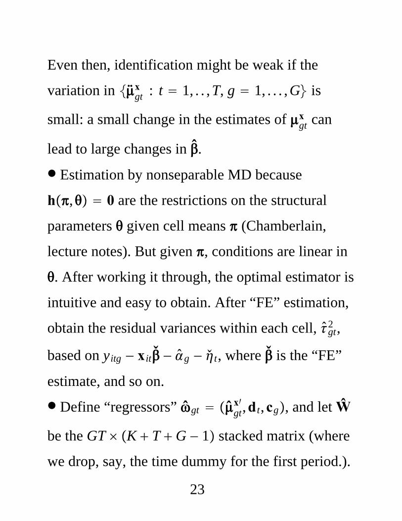
Even then, identification might be weak if the
variation in gtx : t 1, . . ,T, g 1, . . . ,G is
small: a small change in the estimates of gtx can
lead to large changes in .
∙ Estimation by nonseparable MD because
h, 0 are the restrictions on the structural
parameters given cell means (Chamberlain,
lecture notes). But given , conditions are linear in
. After working it through, the optimal estimator is
intuitive and easy to obtain. After “FE” estimation,
obtain the residual variances within each cell, gt2 ,
based on yitg − xit − g − t, where is the “FE”
estimate, and so on.
∙ Define “regressors” gt gtx′,dt,cg, and let Ŵ
be the GT K T G − 1 stacked matrix (where
we drop, say, the time dummy for the first period.).
23

Let Ĉ be the GT GT diagonal matrix with
gt2 /Ngt/N down the diagonal. The optimal MD
estimator, which is N -asymptotically normal, is
Ŵ ′Ĉ−1Ŵ−1Ŵ ′Ĉ−1y. (51)
As in separable cases, the efficient MD estimator
looks like a “weighted least squares” estimator and
its asymptotic variance is estimated as
Ŵ ′Ĉ−1Ŵ−1/N. (Might be better to use resampling
method here.)
∙ Inoue (2007) obtains a different limiting
distribution, which is stochastic, because he treats
estimation of gtx and gt
y asymmetrically.
∙ Deaton (1985), Verbeek and Nijman (1993), and
Collado (1997), use a different asymptotic analysis.
In the current notation, GT → (Deaton) or
24

G → , with the cell sizes fixed.
∙ Allows for models with lagged dependent
variables, but now the vectors of means contain
redundancies. If
yt t yt−1 zt f ut, Eut|g 0, (52)
then the same moments are valid. But, now we
would define the vector of means as gty ,gt
z , and
appropriately pick off gty in defining the moment
conditions. We now have fewer moment conditions
to estimate the parameters.
∙ The MD approach applies to extensions of the
basic model. Random trend model (Heckman and
Hotz (1989)):
yt t xt f1 f2t ut. (53)
gty t gt
x g gt, (54)
25

We can even estimate models with time-varying
factor loads on the heterogeneity:
yt t xt tf ut, (55)
gty t gt
x tg. (56)
∙ How can we use a stronger assumption, such as
Eut|zt, f 0, t 1, . . . ,T, for instruments zt, to
more precisely estimate ? Gives lots of potentially
useful moment conditions:
Ezt′yt|g tEzt
′|g Ezt′xt|g Ezt
′f|g, (57)
using Ezt′ut|g 0.
26